laboratory manual - jawaharlal nehru engineering … · web viewjawaharlal nehru engineering...

Department of Computer Sci. &Engineering

LAB MANUALBE(CSE)

Data Warehousing and Data Mining

MGM's Jawaharlal Nehru Engineering College,

Aurangabad

Jawaharlal Nehru Engineering CollegeAurangabad

Laboratory Manual

Data Warehousing and Data mining

ForFinal Year Students CSE

Dept: Computer Science & Engineering

Author JNEC, Aurangabad

FOREWORD

It is my great pleasure to present this laboratory manual for FINAL YEARCOMPUTER SCIENCE & ENGINEERING students for the subject of Data Warehousing and data mining. As a student, many of you may be wondering about the subject and exactly that has been tried through this manual.

As you may be aware that MGM has already been awarded with ISO 9000 certification and it is our aim to technically equip students taking the advantage of the procedural aspects of ISO 9000 Certification.

Faculty members are also advised that covering these aspects in initial stage itself will relieve them in future as much of the load will be taken care by the enthusiastic energies of the students once they are conceptually clear.

Dr. S.D. Deshmukh

Principal

LABORATORY MANUAL CONTENTS

This manual is intended for FIANL YEAR COMPUTER SECINCE & ENGINEERING students for the subject of Data Warehousing and Data Mining. This manual typically contains practical/Lab Sessions related Data warehousing and data mining covering various aspects related the subject to enhanced understanding.

Students are advised to thoroughly go through this manual rather than only topics mentioned in the syllabus as practical aspects are the key to understanding and conceptual visualization of theoretical aspects covered in the books.

Good Luck for your Enjoyable Laboratory Sessions.

Dr. V.B. Musande Dr. Madhuri S. Joshi Pradeepkumar BhaleHOD, CSE

CSE Dept

DOs and DON’Ts in Laboratory:

1. Make entry in the Log Book as soon as you enter the Laboratory.

2. All the students should sit according to their roll numbers starting from their left to right.

3. All the students are supposed to enter the terminal number in the log book.

4. Do not change the terminal on which you are working.

5. All the students are expected to get at least the algorithm of the program/concept to be implemented.

6. Strictly observe the instructions given by the teacher/Lab Instructor.

Instruction for Laboratory Teachers::

1. Submission related to whatever lab work has been completed should be done during the next lab session. The immediate arrangements for printouts related to submission on the day of practical assignments.

2. Students should be taught for taking the printouts under the observation of lab teacher.

3. The promptness of submission should be encouraged by way of marking and evaluation patterns that will benefit the sincere students.

MGM’s

Jawaharlal Nehru Engineering College, Aurangabad

Department of Computer Science and Engineering

Vision of CSE Department

To develop computer engineers with necessary analytical ability and human values who can creatively design, implement a wide spectrum of computer systems for welfare of the society.

Mission of the CSE Department:Preparing graduates to work on multidisciplinary platforms associated with their professional

position both independently and in a team environment.Preparing graduates for higher education and research in computer science and engineering

enabling them to develop systems for society development.

Programme Educational Objectives

Graduates will be able to

I. To analyze, design and provide optimal solution for Computer Science & Engineering and multidisciplinary problems.

II. To pursue higher studies and research by applying knowledge of mathematics and fundamentals of computer science.

III. To exhibit professionalism, communication skills and adapt to current trends by engaging in lifelong learning.

Programme Outcomes (POs):Engineering Graduates will be able to:

1. Engineering knowledge: Apply the knowledge of mathematics, science, engineering fundamentals, and an engineering specialization to the solution of complex engineering problems.

2. Problem analysis: Identify, formulate, review research literature, and analyze complex engineering problems reaching substantiated conclusions using first principles of mathematics, natural sciences, and engineering sciences.

3. Design/development of solutions: Design solutions for complex engineering problems anddesign system components or processes that meet the specified needs with appropriate consideration for the public health and safety, and the cultural, societal, and environmental considerations.

4. Conduct investigations of complex problems: Use research-based knowledge and research methods including design of experiments, analysis and interpretation of data, and synthesis of the information to provide valid conclusions.

5. Modern tool usage: Create, select, and apply appropriate techniques, resources, and modern engineering and IT tools including prediction and modeling to complex engineering activities with an understanding of the limitations.

6. The engineer and society: Apply reasoning informed by the contextual knowledge to assess societal, health, safety, legal and cultural issues and the consequent responsibilities relevant to the professional engineering practice.

7. Environment and sustainability: Understand the impact of the professional engineering solutions in societal and environmental contexts, and demonstrate the knowledge of, and need for sustainable development.

8. Ethics: Apply ethical principles and commit to professional ethics and responsibilities and norms ofthe engineering practice.

9. Individual and team work: Function effectively as an individual, and as a member or leader in diverse teams, and in multidisciplinary settings.

10. Communication: Communicate effectively on complex engineering activities with the engineering community and with society at large, such as, being able to comprehend and write effective reports and design documentation, make effective presentations, and give and receive clear instructions.

11. Project management and finance: Demonstrate knowledge and understanding of the engineering and management principles and apply these to one’s own work, as a member and leader in a team, to manage projects and in multidisciplinary environments.

12. Life-long learning: Recognize the need for, and have the preparation and ability to engage independent and life-long learning in the broadest context of technological change.

SUBJECT INDEX

Sr. No.

Title Page No.

SET-I

1 Implementation of OLAP operations

2 Implementation of Varying Arrays

3 Implementation of Nested Tables

4 Demonstration of any ETL tool

5 Write a program of Apriori algorithm using any programming language.

6 Write a program of Naive Bayesian classification using C.

7 Write a program of cluster analysis using simple k-means algorithm using any programming language.

8 A case study of Business Intelligence in Government sector/Social Networking/Business.

Sr. No.

Title Page No.

SET-II

1 Create data-set in .arff file format. Demonstration of preprocessing on WEKA data-set.

2 Demonstration of Association rule process on data-set contact lenses.arff /supermarket using apriori algorithm.

3 Demonstration of classification rule process on WEKA data-set using j48 algorithm.

4 Demonstration of classification rule process on WEKA data-set using Naive Bayes algorithm.

5 Demonstration of clustering rule process on data-set iris.arff using simple k-means.

Class: BE(CSE) Subject: Lab I- DWDM (CSE 421)

Experiment No. 1_______________________________________________________________Title: OLAP operations

S/w Requirement: ORACLE

Objectives:

• To learn fundamentals of data warehousing• To learn concepts of dimensional modeling• To learn OLAP operations

Reference:

• SQL‐PL/SQL by Ivan Bayross• Data Mining Concept and Technique By Han & Kamber• Data Warehousing Fundamentals By Paulraj

Pre‐requisite:

• Fundamental Knowledge of Database Management• Fundamental Knowledge of SQL

Description:

OLAP is an acronym for On Line Analytical Processing. An OLAP system manages large amount of historical data, provides facilities for summarization and aggregation, and stores and manages information at different levels of granularity.

OLAP Operations

Since OLAP servers are based on multidimensional view of data, we will discuss OLAP operations in multidimensional data.

Here is the list of OLAP operations:

Roll-up Drill-down Slice and dice Pivot (rotate)

Roll-up

Roll-up performs aggregation on a data cube in any of the following ways:

By climbing up a concept hierarchy for a dimension By dimension reduction

The following diagram illustrates how roll-up works.

Roll-up is performed by climbing up a concept hierarchy for the dimension location. Initially the concept hierarchy was "street < city < province < country". On rolling up, the data is aggregated by ascending the location hierarchy from the level of city to

the level of country. The data is grouped into cities rather than countries. When roll-up is performed, one or more dimensions from the data cube are removed.

Drill-downDrill-down is the reverse operation of roll-up. It is performed by either of the following ways:

By stepping down a concept hierarchy for a dimension By introducing a new dimension.

The following diagram illustrates how drill-down works:

Drill-down is performed by stepping down a concept hierarchy for the dimension time.

Initially the concept hierarchy was "day < month < quarter < year." On drilling down, the time dimension is descended from the level of quarter to

the level of month. When drill-down is performed, one or more dimensions from the data cube are

added. It navigates the data from less detailed data to highly detailed data.

SliceThe slice operation selects one particular dimension from a given cube and provides a new sub-cube. Consider the following diagram that shows how slice works.

Here Slice is performed for the dimension "time" using the criterion time = "Q1".

It will form a new sub-cube by selecting one or more dimensions.

DiceDice selects two or more dimensions from a given cube and provides a new sub-cube. Consider the following diagram that shows the dice operation.

The dice operation on the cube based on the following selection criteria involves three dimensions.

(location = "Toronto" or "Vancouver")

(time = "Q1" or "Q2")

(item =" Mobile" or "Modem")

PivotThe pivot operation is also known as rotation. It rotates the data axes in view in order to provide an alternative presentation of data. Consider the following diagram that shows the pivot operation.

Post lab assignment: Answer the following Questions/Points

1. Star schema vs snowflake schema2. Dimensional table Vs. Relational Table3. Advantages of snowflake schema

Conclusion:

Through OLAP operations the data can be extracted in different fashion. This helps further to analyze data as per the requirement.

*****


Experiment No. 2_______________________________________________________________Title: Implementation of Varying Arrays


Objectives:

• To learn fundamentals of var arrays

Reference:

• SQL‐PL/SQL by Ivan Bayrose• Data Mining Concept and Technique By Han & Kamber• Data Warehousing Fundamentals By Paulraj

Pre‐requisite:


Theory:

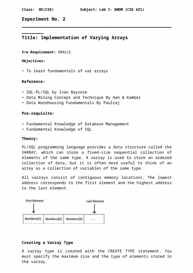
PL/SQL programming language provides a data structure called the VARRAY, which can store a fixed-size sequential collection of elements of the same type. A varray is used to store an ordered collection of data, but it is often more useful to think of an array as a collection of variables of the same type.

All varrays consist of contiguous memory locations. The lowest address corresponds to the first element and the highest address to the last element.

Creating a Varray Type

A varray type is created with the CREATE TYPE statement. You must specify the maximum size and the type of elements stored in the varray.

The basic syntax for creating a VRRAY type at the schema level is:

CREATE OR REPLACE TYPE varray_type_name IS VARRAY(n) of <element_type>

Where,

varray_type_name is a valid attribute name, n is the number of elements (maximum) in the varray, element_type is the data type of the elements of the array.

Maximum size of a varray can be changed using the ALTER TYPE statement.

For example,

CREATE Or REPLACE TYPE namearray AS VARRAY(3) OF VARCHAR2(10);/

Type created.

The basic syntax for creating a VRRAY type within a PL/SQL block is:

TYPE varray_type_name IS VARRAY(n) of <element_type>

For example:

TYPE namearray IS VARRAY(5) OF VARCHAR2(10);Type grades IS VARRAY(5) OF INTEGER;

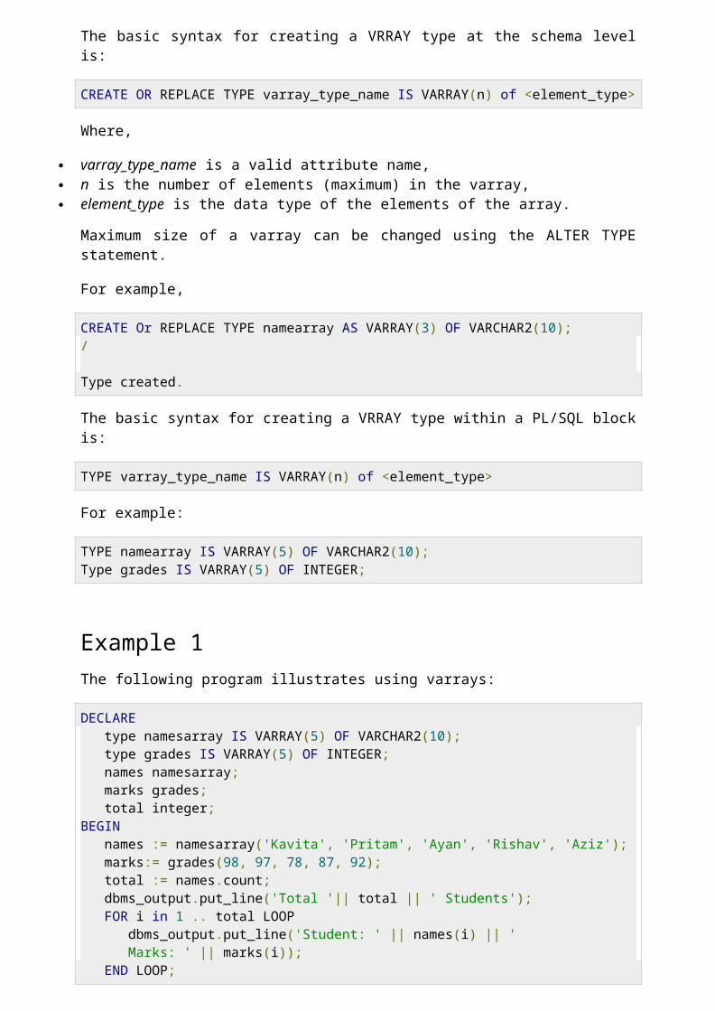
Example 1The following program illustrates using varrays:

DECLARE type namesarray IS VARRAY(5) OF VARCHAR2(10); type grades IS VARRAY(5) OF INTEGER; names namesarray; marks grades; total integer;BEGIN names := namesarray('Kavita', 'Pritam', 'Ayan', 'Rishav', 'Aziz'); marks:= grades(98, 97, 78, 87, 92); total := names.count; dbms_output.put_line('Total '|| total || ' Students'); FOR i in 1 .. total LOOP dbms_output.put_line('Student: ' || names(i) || ' Marks: ' || marks(i)); END LOOP;END;/

When the above code is executed at SQL prompt, it produces the following result:

Student: Kavita Marks: 98Student: Pritam Marks: 97Student: Ayan Marks: 78Student: Rishav Marks: 87Student: Aziz Marks: 92

PL/SQL procedure successfully completed.

Note:

In oracle environment, the starting index for varrays is always 1. You can initialize the varray elements using the constructor method of the varray type, which

has the same name as the varray. Varrays are one-dimensional arrays. A varray is automatically NULL when it is declared and must be initialized before its elements

can be referenced.

Post lab assignment:

1. Advantages of varrays

Conclusion:

I have understood the process of creating and handling the varying arrays.

*****


Experiment No. 3_______________________________________________________________Title: Implementation of Nested Tables


Objective:

• To learn fundamentals of Nested Arrays

Reference:

• SQL‐PL/SQL by Ivan Bayross• Data Mining Concept and Technique By Han & Kamber• Data Warehousing Fundamentals By Paulraj

Pre‐requisite:


A collection is an ordered group of elements having the same data type. Each element is identified by a unique subscript that represents its position in the collection.

PL/SQL provides three collection types:

Index-by tables or Associative array Nested table Variable-size array or Varray

Oracle documentation provides the following characteristics for each type of collections:

Collection Type Number of Elements

Subscript Type

Dense or Sparse Where Created

Can Be Object Type Attribute

Associative array (or index-by table) UnboundedString or integer

EitherOnly in PL/SQL block

No

Nested table Unbounded IntegerStarts dense, can become sparse

Either in PL/SQL block or at schema level

Yes

Variable-size array (Varray) Bounded IntegerAlways dense

Either in PL/SQL block or at schema level

Yes

We have already discussed varray in the chapter 'PL/SQL arrays'. In this chapter, we will discuss PL/SQL tables.

Both types of PL/SQL tables, i.e., index-by tables and nested tables have the same structure and their rows are accessed using the subscript notation. However, these two types of tables differ in one aspect; the nested tables can be stored in a database column and the index-by tables cannot.

Index-By TableAn index-by table (also called an associative array) is a set of key-value pairs. Each key is unique and is used to locate the corresponding value. The key can be either an integer or a string.An index-by table is created using the following syntax. Here, we are creating an index-by table namedtable_name whose keys will be of subscript_type and associated values will be of element_type

TYPE type_name IS TABLE OF element_type [NOT NULL] INDEX BY subscript_type;

table_name type_name;

Example:

Following example shows how to create a table to store integer values along with names and later it prints the same list of names.

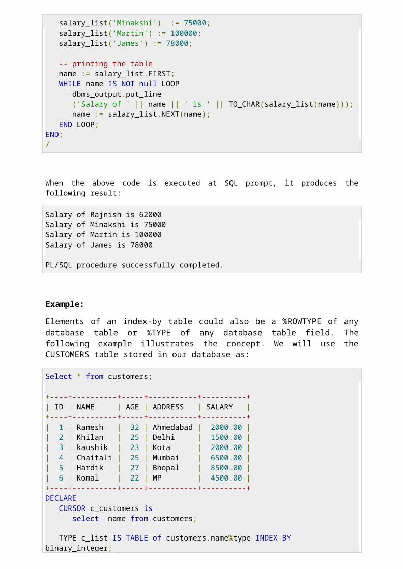
DECLARE TYPE salary IS TABLE OF NUMBER INDEX BY VARCHAR2(20); salary_list salary; name VARCHAR2(20);BEGIN -- adding elements to the table salary_list('Rajnish') := 62000; salary_list('Minakshi') := 75000; salary_list('Martin') := 100000; salary_list('James') := 78000;

-- printing the table name := salary_list.FIRST; WHILE name IS NOT null LOOP dbms_output.put_line ('Salary of ' || name || ' is ' || TO_CHAR(salary_list(name))); name := salary_list.NEXT(name); END LOOP;END;/


Salary of Rajnish is 62000Salary of Minakshi is 75000Salary of Martin is 100000Salary of James is 78000


Example:

Elements of an index-by table could also be a %ROWTYPE of any database table or %TYPE of any database table field. The following example illustrates the concept. We will use the CUSTOMERS table stored in our database as:

Select * from customers;

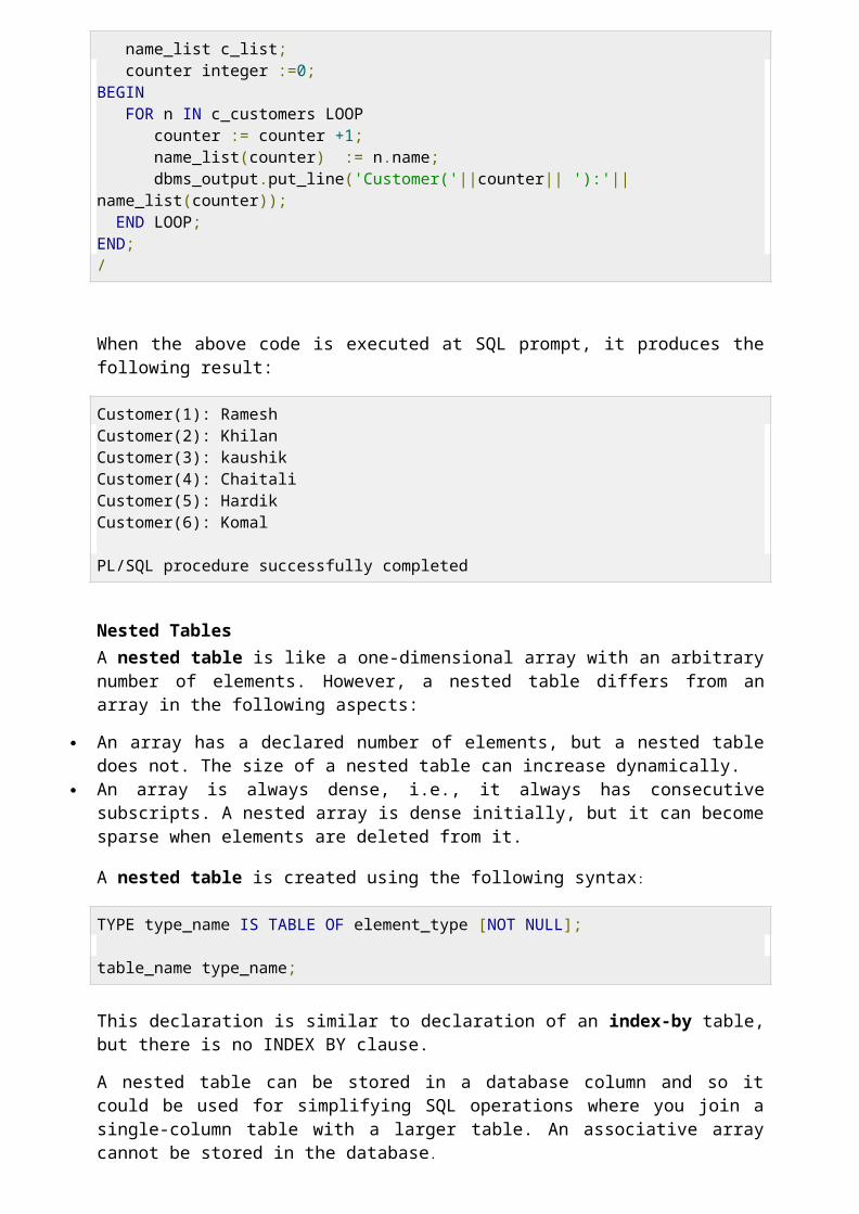
+----+----------+-----+-----------+----------+| ID | NAME | AGE | ADDRESS | SALARY |+----+----------+-----+-----------+----------+| 1 | Ramesh | 32 | Ahmedabad | 2000.00 || 2 | Khilan | 25 | Delhi | 1500.00 || 3 | kaushik | 23 | Kota | 2000.00 || 4 | Chaitali | 25 | Mumbai | 6500.00 || 5 | Hardik | 27 | Bhopal | 8500.00 || 6 | Komal | 22 | MP | 4500.00 |+----+----------+-----+-----------+----------+DECLARE CURSOR c_customers is select name from customers; TYPE c_list IS TABLE of customers.name%type INDEX BY binary_integer; name_list c_list; counter integer :=0;BEGIN FOR n IN c_customers LOOP counter := counter +1; name_list(counter) := n.name; dbms_output.put_line('Customer('||counter|| '):'||name_list(counter)); END LOOP;END;/


Customer(1): Ramesh Customer(2): Khilan Customer(3): kaushik Customer(4): Chaitali Customer(5): Hardik Customer(6): Komal

PL/SQL procedure successfully completed

Nested TablesA nested table is like a one-dimensional array with an arbitrary number of elements. However, a nested table differs from an array in the following aspects:

An array has a declared number of elements, but a nested table does not. The size of a nested table can increase dynamically.

An array is always dense, i.e., it always has consecutive subscripts. A nested array is dense initially, but it can become sparse when elements are deleted from it.

A nested table is created using the following syntax:

TYPE type_name IS TABLE OF element_type [NOT NULL];

table_name type_name;

This declaration is similar to declaration of an index-by table, but there is no INDEX BY clause.

A nested table can be stored in a database column and so it could be used for simplifying SQL operations where you join a single-column table with a larger table. An associative array cannot be stored in the database.

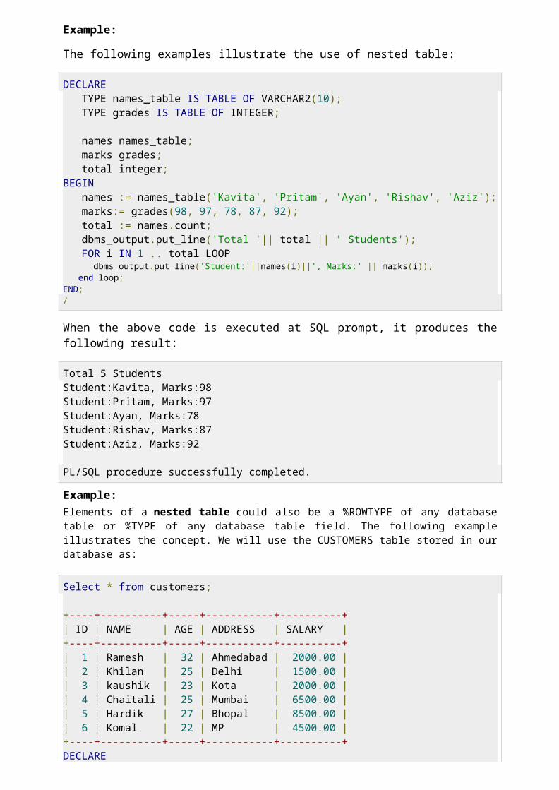
Example:

The following examples illustrate the use of nested table:

DECLARE TYPE names_table IS TABLE OF VARCHAR2(10); TYPE grades IS TABLE OF INTEGER;

names names_table; marks grades; total integer;BEGIN names := names_table('Kavita', 'Pritam', 'Ayan', 'Rishav', 'Aziz'); marks:= grades(98, 97, 78, 87, 92); total := names.count; dbms_output.put_line('Total '|| total || ' Students'); FOR i IN 1 .. total LOOP dbms_output.put_line('Student:'||names(i)||', Marks:' || marks(i)); end loop;END;/


Total 5 StudentsStudent:Kavita, Marks:98Student:Pritam, Marks:97Student:Ayan, Marks:78Student:Rishav, Marks:87Student:Aziz, Marks:92


Example:Elements of a nested table could also be a %ROWTYPE of any database table or %TYPE of any database table field. The following example illustrates the concept. We will use the CUSTOMERS table stored in our database as:

Select * from customers;

+----+----------+-----+-----------+----------+| ID | NAME | AGE | ADDRESS | SALARY |+----+----------+-----+-----------+----------+| 1 | Ramesh | 32 | Ahmedabad | 2000.00 || 2 | Khilan | 25 | Delhi | 1500.00 || 3 | kaushik | 23 | Kota | 2000.00 || 4 | Chaitali | 25 | Mumbai | 6500.00 || 5 | Hardik | 27 | Bhopal | 8500.00 || 6 | Komal | 22 | MP | 4500.00 |+----+----------+-----+-----------+----------+

DECLARE CURSOR c_customers is SELECT name FROM customers;

TYPE c_list IS TABLE of customers.name%type; name_list c_list := c_list(); counter integer :=0;BEGIN FOR n IN c_customers LOOP counter := counter +1; name_list.extend; name_list(counter) := n.name; dbms_output.put_line('Customer('||counter||'):'||name_list(counter)); END LOOP;END;/


Customer(1): Ramesh Customer(2): Khilan Customer(3): kaushik Customer(4): Chaitali Customer(5): Hardik Customer(6): Komal


Conclusion:

I have understood the process of creating and handling the Nested Tables. It is different from the tables we handled so far.

*****


Experiment No. 4_______________________________________________________________Title: Demonstration of any ETL tool

Objectives: To learn ETL Tool.

Instructions:

1. Search the web for popular ETL tools. Read at least two ETL tools.

2. Describe One ETL Tool with its salient features.

Conclusion:

Conclude about the ETL tool you described.

*****


Experiment No. 5_______________________________________________________________Title: Implement Apriori algorithm for association rule

Objectives:

To learn Apriori algorithm for data association

Reference:• Data Mining Introductory & Advanced Topic by Margaret H. Dunham• Data Mining Concept and Technique By Han & Kamber

Pre‐requisite:• Fundamental Knowledge of Database Management

Theory:Association rule mining is to find out association rules that satisfy the predefinedminimum support and confidence from a given database. The problem is usuallydecomposed into two sub problems.

Find those item sets whose occurrences exceed a predefined threshold in the database; those item sets are called frequent or large item sets.

Generate association rules from those large item sets with the constraints of minimal confidence.

Suppose one of the large item sets is Lk = {I1,I2,...,Ik}; association rules with this item setsare generated in the following way: the first rule is {I1,I2,...,Ik − 1} = > {Ik}. By checkingthe confidence this rule can be determined as interesting or not. Then, other rules aregenerated by deleting the last items in the antecedent and inserting it to the consequent,further the confidences of the new rules are checked to determine the interestingness ofthem. This process iterates until the antecedent becomes empty.

Since the second sub problem is quite straight forward, most of the research focuses onthe first sub problem. The Apriori algorithm finds the frequent sets L in Database D.

Find frequent set Lk − 1. Join Step.

Ck is generated by joining Lk − 1with itself Prune Step.

Any (k − 1) ‐itemset that is not frequent cannot be a subset of a frequent k ‐ itemset, hence should be removed.

where (Ck: Candidate itemset of size k) (Lk: frequent itemset of size k)

Input :A large supermarket tracks sales data by SKU( Stoke Keeping Unit) (item), and thus isable to know what items are typically purchased together. Apriori is a moderatelyefficient way to build a list of frequent purchased item pairs from this data.

Let the database of transactions consist of the sets {1,2,3,4}, {2,3,4}, {2,3}, {1,2,4}, {1,2,3,4},and {2,4}.

OutputEach number corresponds to a product such as "butter" or "water". The first step ofApriori to count up the frequencies, called the supports, of each member item separately:

Item Support1 32 63 44 5

We can define a minimum support level to qualify as "frequent," which depends on thecontext. For this case, let min support = 3. Therefore, all are frequent. The next step is togenerate a list of all 2-pairs of the frequent items. Had any of the above items not beenfrequent, they wouldn't have been included as a possible member of possible 2-item pairs.In this way, Apriori prunes the tree of all possible sets.

Item Support{1,2} 3{1,3} 2{1,4} 3{2,3} 4{2,4} 5{3,4} 3

This is counting up the occurrences of each of those pairs in the database. Sinceminsup=3, we don't need to generate 3-sets involving {1,3}. This is because since they'renot frequent, no supersets of them can possibly be frequent. Keep going:

Item Support{1,2,4} 3{2,3,4} 3

Post lab assignment:1. Give an example for Apriori with transaction and explain Apriori-gen-algorithm

Conclusion:

Apriori Algorithm works on the principle of frequent itemsets, support and confidence. We can generate association rules and mine the basic data from a database.

*****


Experiment No. 6_______________________________________________________________Title: Bayesian Classification

Objective:

• To implement classification using Bayes theorm.


Pre‐requisite:• Fundamental Knowledge of probability and Bayes theorm

Theory:

The simple baysian classification assumes that the effect of an attribute value of a givenclass membership is independent of other attribute.

The Bayes theorm is as follows –Let X be an unknown sample. Let it be hypothesis such that X belongs to particular class C. We need to determine P(H/X).

The probability that hypothesis it holds is given that all values of X are observed.

P(H/X) = P(X/H).P(H)/P(X)

In this program, we initially take the number of tuples in training data set in variable L.The string array’s name, gender, hight, output to store the details and output respectfully.Therefore, the tuple details are taken from user using ‘for’ loops.

Bayesian classification has an expected classification. Now using the counter variablesfor various attributes i.e. (male/female) for gender and (short/medium/tall) for hight.

The tuples are scanned and the respective counter is incremented accordingly using ifelse-if structure.

Therefore variables pshort, pmed, plong are used to convert the counter variables tocorresponding values.

Algorithm –3. START4. Store the training data set5. Specify ranges for classifying the data6. Calculate the probability of being tall, medium, short7. Also, calculate the probabilities of tall, short, medium according to gender and

Classification ranges 6. Calculate the likelihood of short, medium and tall

7. Calculate P(t) by summing up of probable likelihood 8. Calculate actual probabilities

Input:

Training data set

Name Gender Height OutputChristina F 1.6m ShortJim M 1.9m TallMaggie F 1.9m MediumMartha F 1.88m MediumStephony F 1.7m MediumBob M 1.85m ShortDave M 1.7m ShortSteven M 2.1m TallAmey F 1.8m Medium

OutputThe tuple belongs to the class having highest probability. Thus new tuple is classified.

Conclusion:

Bayes classification uses probability theory. Hence it is known as a statistical classifier.

*****


Experiment No. 7_______________________________________________________________Title: Demonstration of any ETL tool

Objectives: To understand principles of clustering To Implement K‐means algorithm for clustering


Pre‐requisite:• Fundamental Knowledge of Database Management

Theory:

In statistics and machine learning, k‐means clustering is a method of cluster analysis which aims to partition n observations into k clusters in which each observation belongs to the cluster with the nearest mean.‐Mean Clustering algorithm works?Here is step by step k means clustering algorithm:

Step 1. Begin with a decision on the value of k = number of clusters

Step 2. Put any initial partition that classifies the data into k clusters. You may assign thetraining samples randomly, or systematically as the following:

1. Take the first k training sample as single‐element clusters

Assign each of the remaining (N-k) training sample to the cluster with the nearestcentroid. After each assignment, recomputed the centroid of the gaining cluster.

Step 3. Take each sample in sequence and compute its distance from the centroid of eachof the clusters. If a sample is not currently in the cluster with the closest centroid, switchthis sample to that cluster and update the centroid of the cluster gaining the new sampleand the cluster losing the sample.

Step 4. Repeat step 3 until coverage is achieved, that is until a pass through the training sample cause no new assignment

Note: You can implement above problem no 3 to 6 in C/C++/JAVA

Conclusion:

K- means clustering is simplest method used for forming data clusters.*****


Experiment No. 8_______________________________________________________________Title: A case study of Business Intelligence in Government sector/Social Networking/Business

Objectives:

To understand the concept of BI

To understand the Role of Data Analyst in Business

Instructions:

Analyze the Case Study: Closure of Big Bazaar in Aurangabad

Points: 1. Potential of starting Big Bazar in Aurangabad2. How people responded3. What was the role of data analyst4. How the data was maintained through daily transactions?5. What were the weak points?

*****


Experiment No. 1_______________________________________________________________Title: Demonstration of preprocessing on dataset student.arff

Objectives:

To learn to use the Weka machine learning toolkit

ReferencesWitten, Ian and Eibe, Frank. Data Mining: Practical Machine Learning Tools and Techniques.Springer.

RequirementsHow do you load Weka?1. What options are available on main panel?2. What is the purpose of the the following in Weka:

1. The Explorer2. The Knowledge Flow interface3. The Experimenter4. The command‐line interface5. Describe the arff file format.

Steps of execution:

Step1: Loading the data. We can load the dataset into weka by clicking on open button in preprocessing interface and selecting the appropriate file.

Step2: Once the data is loaded, weka will recognize the attributes and during the scan of the data weka will compute some basic strategies on each attribute. The left panel in the above figure shows the list of recognized attributes while the top panel indicates the names of the base relation or table and the current working relation (which are same initially).

Step3: Clicking on an attribute in the left panel will show the basic statistics on the attributes for the categorical attributes the frequency of each attribute value is shown, while for continuous attributes we can obtain min, max, mean, standard deviation and deviation etc.,

Step4: The visualization in the right button panel in the form of cross-tabulation across two attributes.

Note: we can select another attribute using the dropdown list

Step5: Selecting or filtering attributes

R e m oving an attribut e - When we need to remove an attribute, we can do this by using the attribute filters in weka. In the filter model panel, click on choose button, This will show a popup window with a list of available filters.

Scroll down the list and select the “weka filters unsupervised Attribute remove” filters.

Step 6: a) Next click the textbox immediately to the right of the choose button. In the resulting dialog box enter the index of the attribute to be filtered out.

b) Make sure that invert selection option is set to false. The click OK now in the filter box you will see “Remove-R-7”.

c) Click the apply button to apply filter to this data. This will remove the attribute and create new working relation.

d) Save the new working relation as an arff file by clicking save button on the top (button) panel(student.arff)

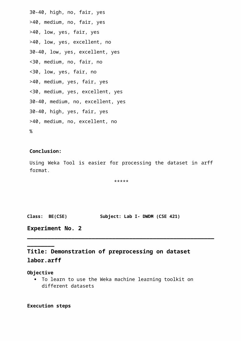
Dataset student .arff

@relation student

@attribute age {<30,30-40,>40}

@attribute income {low, medium, high}

@attribute student {yes, no}

@attribute credit-rating {fair, excellent}

@attribute buyspc {yes, no}

@data

%

<30, high, no, fair, no

<30, high, no, excellent, no

30-40, high, no, fair, yes

>40, medium, no, fair, yes

>40, low, yes, fair, yes

>40, low, yes, excellent, no

30-40, low, yes, excellent, yes

<30, medium, no, fair, no

<30, low, yes, fair, no

>40, medium, yes, fair, yes

<30, medium, yes, excellent, yes

30-40, medium, no, excellent, yes

30-40, high, yes, fair, yes

>40, medium, no, excellent, no

%

Conclusion:

Using Weka Tool is easier for processing the dataset in arff format.

*****


Experiment No. 2_______________________________________________________________Title: Demonstration of preprocessing on dataset labor.arff

Objective To learn to use the Weka machine learning toolkit on different datasets

Execution steps

Step1: Loading the data. We can load the dataset into weka by clicking on open button in preprocessing interface and selecting the appropriate file.

Step2: Once the data is loaded, weka will recognize the attributes and during the scan of the data weka will compute some basic strategies on each attribute. The left panel in the above figure shows the list of recognized attributes while the top panel indicates the names of the base relation or table and the current working relation (which are same initially).

Step3: Clicking on an attribute in the left panel will show the basic statistics on the attributes for the categorical attributes the frequency of each attribute value is shown, while for continuous attributes we can obtain min, max, mean, standard deviation and deviation etc.,

Step4: The visualization in the right button panel in the form of cross-tabulation across two attributes.

Note: we can select another attribute using the dropdown list

Step5: Selecting or filtering attributes

Removing an attribute- When we need to remove an attribute, we can do this by using the attribute filters in weka. In the filter model panel, click on choose button, This will show a popup window with a list of available filters.Scroll down the list and select the “weka filters unsupervised attribute remove” filters.

Step 6: a) Next click the textbox immediately to the right of the choose button. In the resulting dialog box enter the index of the attribute to be filtered out.

b) Make sure that invert selection option is set to false. The click OK now in the filter box. you will see “Remove-R-7”.

c) Click the apply button to apply filter to this data. This will remove the attribute and create new working relation.

d) Save the new working relation as an arff file by clicking save button on the top(button)panel.(labor.arff)

Conclusion:

Using Weka Tool is easier for processing the dataset in arff format. We practiced it with labor.arff file.

*****


Experiment No. 3_______________________________________________________________Title: Demonstration of Association rule process on dataset contactlenses.arff using apriori algorithm

Objective:To learn to use the Weka toolkit for Association Rule Mining

Execution steps

Step1: Open the data file in Weka Explorer. It is presumed that the required data fields have been discretized. In this example it is age attribute.

Step2: Clicking on the associate tab will bring up the interface for association rule

algorithm.

Step3: We will use apriori algorithm. This is the default algorithm.

Step4: Inorder to change the parameters for the run (example support, confidence etc) we click on the text box immediately to the right of the choose button.

Dataset contactlenses.arff

Dataset test.arff

@relation test

@attribute admissionyear {2005,2006,2007,2008,2009,2010}

@attribute course {cse,mech,it,ece}

@data

%

2005, cse

2005, it

2005, cse

2006, mech

2006, it

2006, ece

2007, it

2007, cse

2008, it

2008, cse

2009, it

2009, ece

%

The following screenshot shows the association rules that were generated when Apriori algorithm is applied on the given dataset.

Conclusion:

The experiment displays Set of large itemsets, best rule found for the given support and the confidence values. We get the results faster using the toolkits.

*****


Experiment No. 4_______________________________________________________________Title: Demonstration of classification rule process on dataset student.arff using j48 algorithm

Objective:To learn to use the Weka machine learning toolkit for j48, decision tree classifier

Steps involved in this experiment:

Step-1: We begin the experiment by loading the data (student.arff)into weka.

Step2: Next we select the “classify” tab and click “choose” button t o select the

“j48”classifier.

Step3: Now we specify the various parameters. These can be specified by clicking in the text box to the right of the chose button. In this example, we accept the default values. The default version does perform some pruning but does not perform error pruning.

Step4: Under the “text” options in the main panel. We select the 10-fold cross validation as our evaluation approach. Since we don’t have separate evaluation data set, this is necessary to get a reasonable idea of accuracy of generated model.

Step-5: We now click ”start” to generate the model .the Ascii version of the tree as well as evaluation statistic will appear in the right panel when the model construction is complete.

Step-6: Note that the classification accuracy of model is about 69%.this indicates that we may find more work. (Either in preprocessing or in selecting current parameters for the classification)

Step-7: Now weka also lets us a view a graphical version of the classification tree. This can be done by right clicking the last result set and selecting “visualize tree” from the pop-up menu.

Step-8: We will use our model to classify the new instances.

Step-9: In the main panel under “text” options click the “supplied test set” radio button and then click the “set” button. This wills pop-up a window which will allow you to open the file containing test instances.

Dataset student .arff

@relation student@attribute age {<30,30-40,>40}

@attribute income {low, medium, high}@attribute student {yes, no}@attribute credit-rating {fair, excellent}@attribute buyspc {yes, no}@data%<30, high, no, fair, no<30, high, no, excellent, no30-40, high, no, fair, yes>40, medium, no, fair, yes>40, low, yes, fair, yes>40, low, yes, excellent, no30-40, low, yes, excellent, yes<30, medium, no, fair, no<30, low, yes, fair, no>40, medium, yes, fair, yes<30, medium, yes, excellent, yes30-40, medium, no, excellent, yes30-40, high, yes, fair, yes>40, medium, no, excellent, no%

The following screenshot shows the classification rules that were generated when j48 algorithm is applied on the given dataset.

Conclusion:

The experiment displays decision tree, which is annotated (labeled). It also gives the time taken to build the tree and the confusion matrix.

*****


Experiment No. 5_______________________________________________________________Title: Demonstration of clustering rule process on data-set iris.arff using simple k-means.

ObjectiveTo learn to use the Weka machine learning toolkit for simple k-means clustering

Execution steps

Step 1: Run the Weka explorer and load the data file iris.arff in preprocessing interface.

Step 2: Inorder to perform clustering select the ‘cluster’ tab in the explorer and click on the choose button. This step results in a dropdown list of available clustering algorithms.

Step 3: In this case we select ‘simple k-means’.

Step 4: Next click in text button to the right of the choose button to get popup window shown in the screenshots. In this window we enter six on the number of clusters and we leave the value of the seed on as it is. The seed value is used in generating a random number which is used for making the internal assignments of instances of clusters.

Step 5: Once of the option have been specified. We run the clustering algorithm there we must make sure that they are in the ‘cluster mode’ panel. The use of training set option is selected and then we click ‘start’ button. This process and resulting window are shown in the following screenshots.

Step 6: The result window shows the centroid of each cluster as well as statistics on the number and the percent of instances assigned to different clusters. Here clusters centroid are means vectors for each clusters. These clusters can be used to characterized the cluster. For eg, the centroid of cluster1 shows the class iris.versicolor mean value of the sepal length is 5.4706, sepal width 2.4765, petal width 1.1294, petal length 3.7941.

Step 7: Another way of understanding characteristics of each cluster through visualization, we can do this, try right clicking the result set on the result. List panel and selecting the visualize cluster.

Step 8: We can assure that resulting dataset which included each instance along with its assign cluster. To do so we click the save button in the visualization window and save the result iris k-mean .The top portion of this file is shown in the following figure

The following screenshot shows the clustering rules that were generated when simple k means algorithm is applied on the given dataset

Conclusion: The k means clustering is able the cluster the data in the iris database.

*****

laboratory manual - jawaharlal nehru engineering … · web viewjawaharlal nehru engineering...

Documents