lagging poor areas: a case study of the south-west china poverty reduction project martin ravallion...

Lagging Poor Areas: A Case Study of the South-West China

Poverty Reduction Project

Martin Ravallion* Development Research Group, World Bank

* based on joint work with Shaohua Chen and Ren Mu, and in collaboration with China’s National Bureau of Statistics

“So, did we have any impact on poverty?”

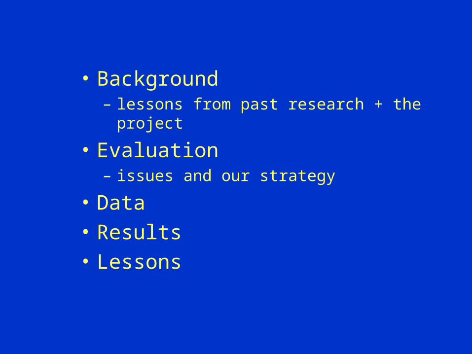
• Background– lessons from past research + the project

• Evaluation– issues and our strategy

• Data

• Results

• Lessons

China: overall success against chronic poverty, but lagging areas

• “Development must be inegalitarian because it does not start in every part of the country at the same time” (W. Arthur Lewis)

• Large reduction in absolute income poverty in China over 1980-2000.– 53% poor in 1981; 8% in 2001

• But wide geographic disparities have emerged, notably between the coast and remote resource-poor inland

• Pattern of growth (sector and place) has been an important factor in overall poverty reduction.– ¾ of overall poverty reduction due to rural areas– “urban bias” meant lower poverty reduction

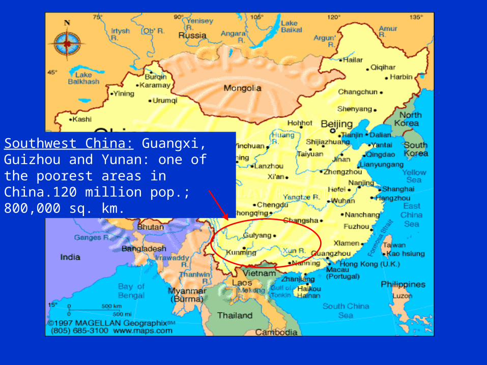
Southwest China: Guangxi, Guizhou and Yunan: one of the poorest areas in China.120 million pop.; 800,000 sq. km.

Lessons from past research in this setting

• Externalities: local infrastructure and the composition of local economic activity have impacts at the farm-household level (Ravallion).

• Rural under-development stems from under-investment in externality-generating activities, esp., agriculture and (less so) non-farm activities.

• Virtuous cycles: a well-targeted external growth stimulus in a poor area can generate positive and more widely diffused income gains over time.

Past research cont.,

• Risk and insurance: – Poor people tend to be less well insured. – Income risk affects portfolio behavior: more liquid wealth

(though more so for middle-income groups) (Jalan and Ravallion)

• Some heterogeneity within poor areas– Villages within the same poor counties need not be good

counter-factuals for the project villages – Evidence for Yunnan =>

.

<5%5%-10%

10%-15%

15%-20%

>=30%

20%-30%

Yunnan: County poverty incidence

N=126

<5%5%-10%

10%-15%

15%-20%

>=30%

20%-30%

Township poverty incidence

N=1571

Past research cont.,

• Poor-area programs: – Government’s emphasis on agriculture makes sense

given that this is a major income component and generator of positive externalities (Ravallion).

– Adequate (human and physical) infrastructure is a pre-condition for growth in poor areas (Jalan & Ravallion).

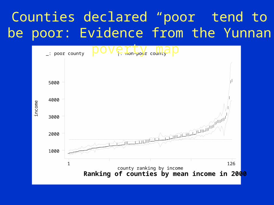
– Counties declared “poor” do tend to be poor• Evidence from probits based on RHS sample data (J&R)• Evidence from the Yunnan poverty map =>

.

_: poor county |: non-poor county

inco

me

Ranking of counties by mean income in 2000county ranking by income

1 126

1000

2000

3000

4000

5000

_______________________________|_____|_____| | |_____|__|_| |_| | | |___|__|____|__|__| | | |__| |__| | |__|__| |_| | |_| | || | | |

| || | | | | |

||

|

|

| |

Counties declared “poor” tend to be poor: Evidence from the Yunnan poverty map

World Bank’s Southwest Poverty Reduction Project

• Rural development programs targeted to poor areas.• Aims to reduce poverty by providing:

• resources to poor farm-households and • social services and rural infrastructure.

• 35 national poor counties • $US 400 million from a World Bank loan and

Chinese government over 1995-2001.

The key components of SWPRP1. Income-generating activities: methods for raising grain

yields, animal husbandry, reforestation.2. Off-farm employment: voluntary labor mobility and

support for township-village enterprises.3. Social services and infrastructure: tuition subsidy to

children from poor families, upgrading village schools and health clinics, rural roads, safe drinking water supply system etc.

4. Institution building and poverty monitoring:– improving the management of the project and – establishing a poverty monitoring system.

Composition of SWPRP spending

% of total investment

Education 8.6 Health 5.4 Labor mobility 9.7 Rural infrastructure 17.2 Agriculture 43.1 Rural enterprise development 11.5 Institution building 1.7 Project & poverty monitoring 2.8 Total 100.0

Uninsured risk remains

• In common with other development projects, the SWPRP provided the capital and technical assistance, but it did not provide insurance

• And many of the project activities are likely to entail non-negligible income risk. The income gains will depend on a number of contingencies:– the vagaries of the weather (given the role of agriculture) – uncertain demand for the new product– risks associated with out migration.

Impact evaluation: generic issues

• Impact is the difference between the relevant outcome indicator with the program and that without it.

• However, we can never simultaneously observe someone in two different states of nature.

• So, while a post-intervention indicator is observed, its value in the absence of the program is not, i.e., it is a counter-factual.

• Time span of evaluation– Development projects may need longer evaluation

periods than found in practice– Expensive longer tracking or more and better data?

• Measurement of welfare impacts– Poor people are not myopic– Consumption may better reveal long-term impact– However, there may be great uncertainty about impact

on permanent income– Lags in impacts on living standards cloud identification

Impact evaluation: specific issues

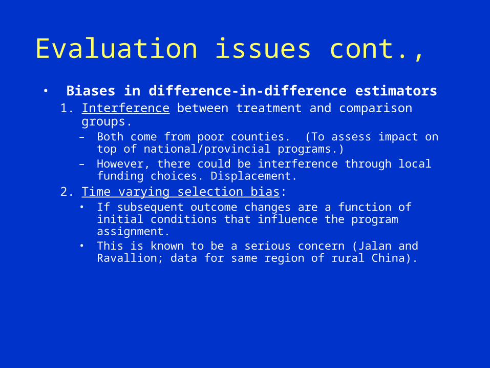
Evaluation issues cont.,

• Biases in difference-in-difference estimators1. Interference between treatment and comparison groups.

– Both come from poor counties. (To assess impact on top of national/provincial programs.)

– However, there could be interference through local funding choices. Displacement.

2. Time varying selection bias: • If subsequent outcome changes are a function of initial

conditions that influence the program assignment. • This is known to be a serious concern (Jalan and Ravallion;

data for same region of rural China).

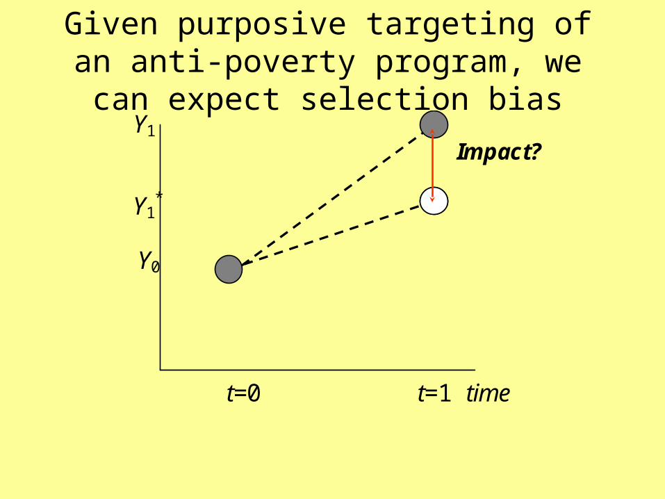
Given purposive targeting of an anti-poverty program, we can expect selection bias

Y1

Impact? Y1

*

Y0

t=0 t=1 time


Y1

Impact

Y1*

Y0

t=0 t=1 time

Observed mean forcomparison group


Y1

Impact

Y1*

Y0

t=0 t=1 time

Selection bias

As long as the bias is additive and time-invariant, diff-in-diff will work ….

Y1

Y1

*

Y0

t=0 t=1 time

But diff-in-diff hides true impact when targeted areas have lower growth prospects.

Y1

Y1

*

Y0

t=0 t=1 time Targeted poor counties in China have lower growth rates

in the absence of intervention (divergence) (Jalan and Ravallion)

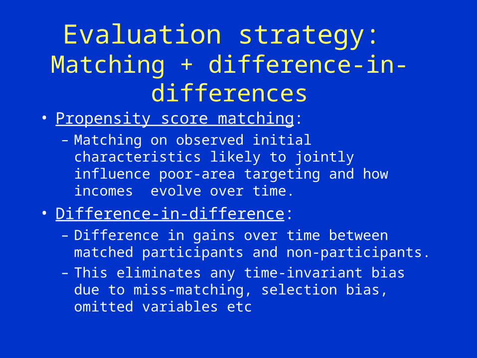
Evaluation strategy: Matching + difference-in-differences

• Propensity score matching: – Matching on observed initial characteristics likely to

jointly influence poor-area targeting and how incomes evolve over time.

• Difference-in-difference: – Difference in gains over time between matched

participants and non-participants.

– This eliminates any time-invariant bias due to miss-matching, selection bias, omitted variables etc

Income and consumption of the i’th project household at date t:

Yit

Yititiit GYDY *)1( ),..,0;,..,1( Ttni

Cit

Cititiit GCDC *)1( ),..,0;,..,1( Ttni

*itY and *

itC : counter-factual income and consumption if the program had not existed.

YitG and C

itG : gains attributable to the project

Yit and C

it : zero-mean innovation error terms

allow for measurement error in itY and itC .

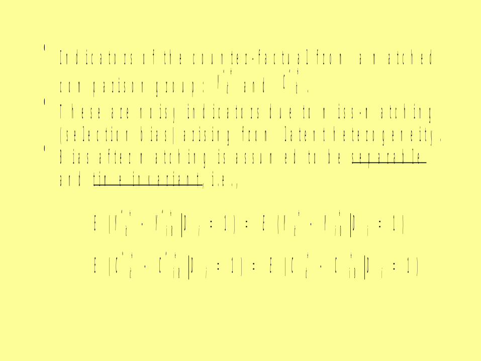
I n d i c a t o r s o f t h e c o u n t e r - f a c t u a l f r o m a m a t c h e d

c o m p a r i s o n g r o u p : *ˆitY a n d *ˆ

itC . T h e s e a r e n o i s y i n d i c a t o r s d u e t o m i s s - m a t c h i n g

( s e l e c t i o n b i a s ) a r i s i n g f r o m l a t e n t h e t e r o g e n e i t y . B i a s a f t e r m a t c h i n g i s a s s u m e d t o b e s e p a r a b l e

a n d t i m e i n v a r i a n t , i . e . ,

)1()1ˆˆ( *0

**0

* iiitiiit DYYEDYYE

)1()1ˆˆ( *0

**0

* iiitiiit DCCEDCCE

T h e n :

)1(]1)ˆ()ˆ[( 0*00

* iY

iY

itiiiitit DGGEDYYYYE

)1(]1)ˆ()ˆ[( 0*

00* i

Ci

Citiiiitit DGGEDCCCCE

W h e n d a t e 0 i s a g e n u i n e b a s e l i n e p r i o r t o t h e i n t e r v e n t i o n ( a n d n o t i n a n y w a y c o n t a m i n a t e d b y t h e

p r o g r a m a s s i g n m e n t ) w e h a v e 000 Ci

Yi GG .

T h e n t h e D D e s t i m a t e s t h e m e a n c u r r e n t g a i n s i n c o n s u m p t i o n a n d i n c o m e f o r p r o g r a m p a r t i c i p a n t s .

W e w i l l c o n s i d e r t h e i m p l i c a t i o n s f o r o u r r e s u l t s o f

t h e p o s s i b i l i t y t h a t 000 Ci

Yi GG .

NBS Rural Household Survey

• Good quality budget and income survey (care in reducing both sampling and non-sampling errors).

• Sampled households maintain a daily record on all transactions + log books on production.

• Local interviewing assistants (resident in the sampled village, or nearby) visit each household at roughly two weekly intervals.

• Inconsistencies found at the local NBS office are checked with the respondents.

• Sample frame: all registered agricultural h’holds.

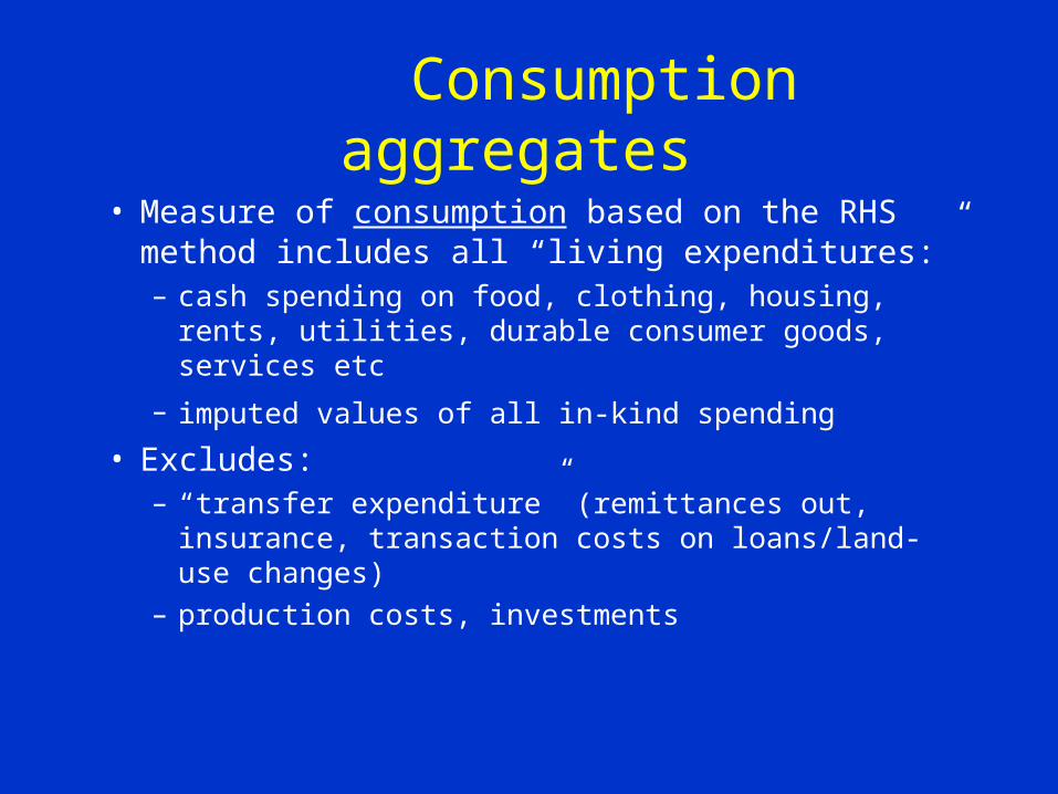
Consumption aggregates

• Measure of consumption based on the RHS method includes all “living expenditures:” – cash spending on food, clothing, housing, rents,

utilities, durable consumer goods, services etc

– imputed values of all in-kind spending

• Excludes: – “transfer expenditure” (remittances out, insurance,

transaction costs on loans/land-use changes)

– production costs, investments

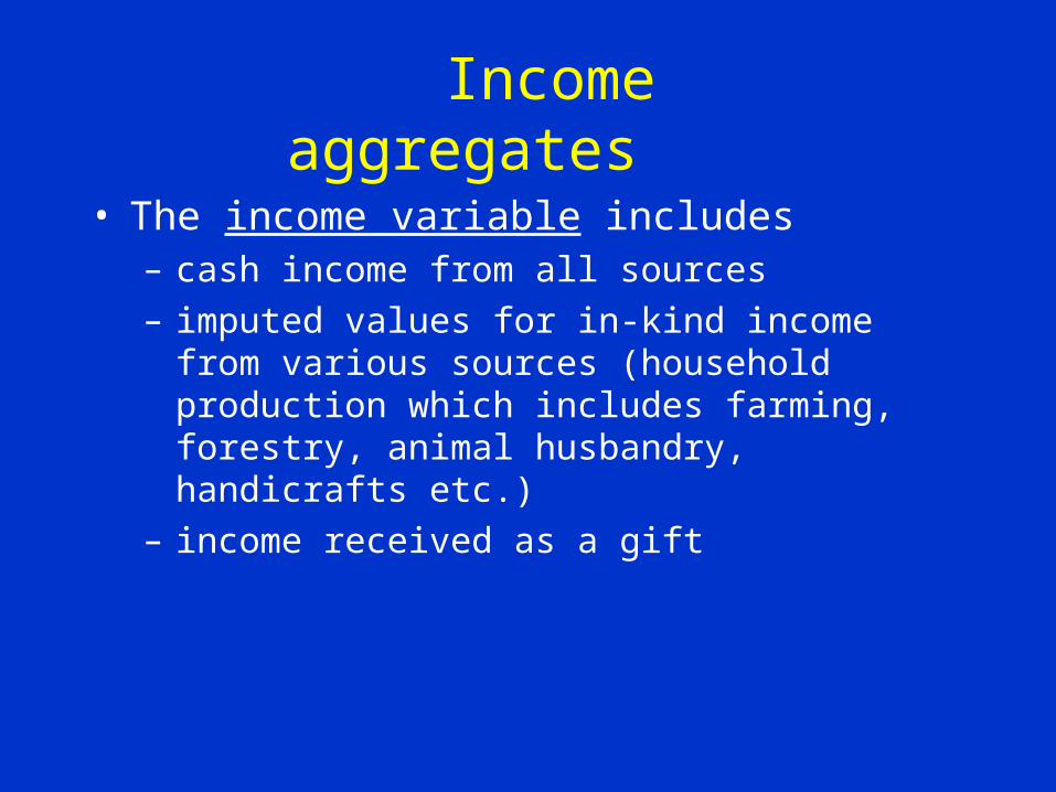
Income aggregates

• The income variable includes– cash income from all sources

– imputed values for in-kind income from various sources (household production which includes farming, forestry, animal husbandry, handicrafts etc.)

– income received as a gift

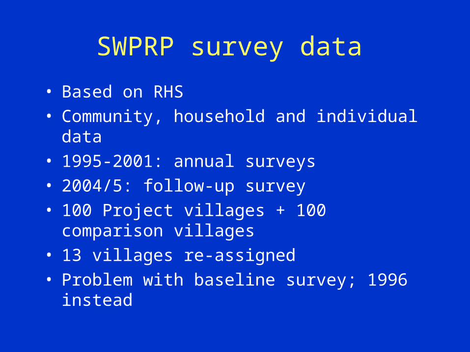
SWPRP survey data

• Based on RHS

• Community, household and individual data

• 1995-2001: annual surveys

• 2004/5: follow-up survey

• 100 Project villages + 100 comparison villages

• 13 villages re-assigned

• Problem with baseline survey; 1996 instead

Descriptive findings

• Project villages started worse off on average than non-project villages, in terms of both income and consumption.

• By the end of the period, the project villages had caught up in mean income, but not consumption.

• This is suggestive of saving from the project’s income gains.

• However, we need to allow for selection bias arising from the program’s purposive targeting.

Covariates of participation• SWPRP villages tend to be:

– in more mountainous remote areas, – less likely to have electricity, – less likely to have a school in the village, – more likely to have a health clinic.

• The project villages tend to have:– higher populations, – lower mean income and – more land per capita, reflecting lower pop. density.

• Consistent with targeting poor villages within poor counties

Matching methods

• No matching: 113 project villages matched with 87 non-project villages (same counties).

• Trimmed comparison group: 113 project villages matched with 71 comparison villages within the outer bounds of the region of common support

• Caliper-bound matching: – Treatment and comparison villages must have an absolute

difference in propensity score < 0.01. – 63 project villages matched with 34 non-project villages.– Raises concern about bias in inferences about the population

of project villages.

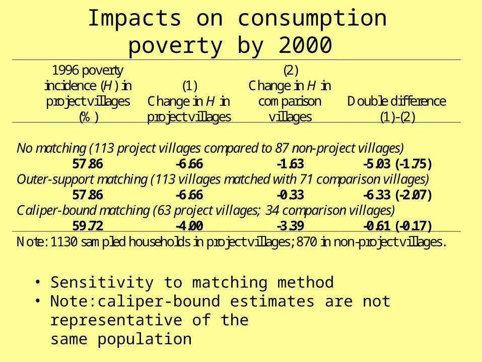
Impacts on consumption poverty by 2000

1996 poverty incidence (H) in project villages

(%)

(1) Change in H in project villages

(2) Change in H in

comparison villages

Double difference (1)-(2)

No matching (113 project villages compared to 87 non-project villages) 57.86 -6.66 -1.63 -5.03 (-1.75) Outer-support matching (113 villages matched with 71 comparison villages)

57.86 -6.66 -0.33 -6.33 (-2.07) Caliper-bound matching (63 project villages; 34 comparison villages)

59.72 -4.00 -3.39 -0.61 (-0.17) Note: 1130 sampled households in project villages; 870 in non-project villages.

• Sensitivity to matching method• Note:caliper-bound estimates are not representative of the

same population

Impacts on consumption poverty by 2004


(%)


(2) Change in H in

comparison villages





• Larger impacts by 2/3 methods

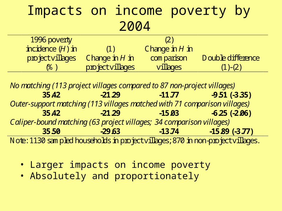
Impacts on income poverty by 2004


(%)


(2) Change in H in

comparison villages





• Larger impacts on income poverty• Absolutely and proportionately

Robustness to choice of poverty line? -2

0-1

8-1

6-1

4-1

2-1

0-8

-6-4

-20

2D

D p

over

ty im

pact

(%

poi

nts)

350 400 450 500 550 600 650 700 750 800 850 900 950 1000105011001150Poverty lines (Yuan per person per year)

trimmed comparison group 2000trimmed comparison group 2004

Impact on consumption poverty

2000

2004

Robustness to choice of poverty line? -2

0-1

8-1

6-1

4-1

2-1

0-8

-6-4

-20

2D

D p

ove

rty

impact

(%

poin

ts)

350 400 450 500 550 600 650 700 750 800 850 900 950 1000105011001150Poverty lines (Yuan per person per year)

trimmed comparison group 2000trimmed comparison group 2004

Impact on income poverty

2000

2004

What have we learnt?

1. Income gains in the disbursement period• The project resulted in an average income gain over five

years of around 10% of baseline mean income,

• representing an average return on the project’s disbursements of about 9-10%.

2. But a large share of the initial income gains was saved

• Half of the cumulative income gain was saved, so that the project’s impact is not evident in current living standards.

What have we learnt?

3. Impacts on poverty remained four years after the end of the project’s disbursements

• Impacts of 6-16% on income poverty rate (depending on matching method)

• But still larger long-term impacts on income poverty than consumption poverty

• Pro-poor impacts on distribution• Impacts on schooling and productive assets

Why the high savings rate?

• When interpreted in terms of the simplest Permanent Income Hypothesis, our results imply that participants felt that a large share of the income gains during the disbursement period was likely to be transient.

• Under simple PIH, the consumption impact of the project identifies the impact on permanent income.

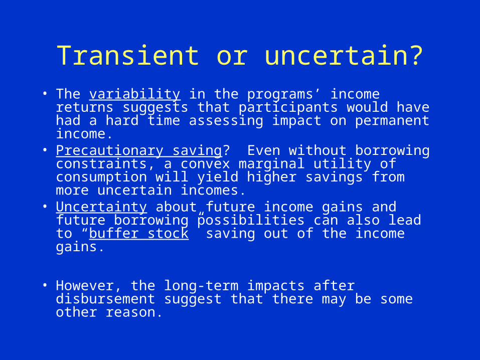
Transient or uncertain?• The variability in the programs’ income returns suggests

that participants would have had a hard time assessing impact on permanent income.

• Precautionary saving? Even without borrowing constraints, a convex marginal utility of consumption will yield higher savings from more uncertain incomes.

• Uncertainty about future income gains and future borrowing possibilities can also lead to “buffer stock” saving out of the income gains.

• However, the long-term impacts after disbursement suggest that there may be some other reason.

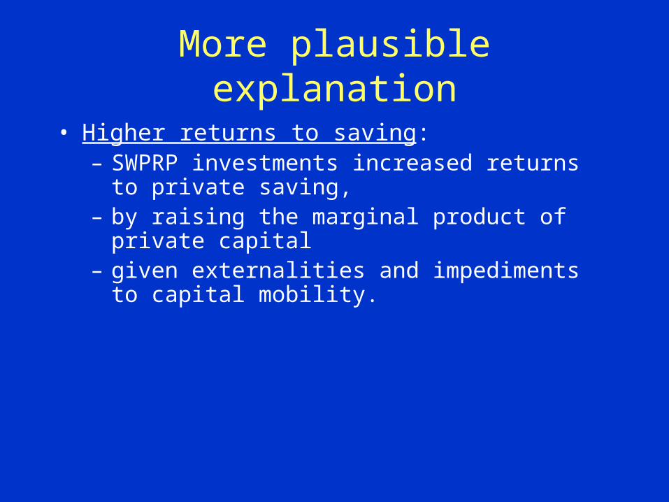
More plausible explanation

• Higher returns to saving: – SWPRP investments increased returns to private

saving, – by raising the marginal product of private capital – given externalities and impediments to capital mobility.

Implications for impact evaluations

A large share of the impact on peoples’ living standards may occur beyond the life of the project. – One option: track welfare impacts over much longer

periods; concerns about feasibility.– Instead look at impacts on partial intermediate indicators

of longer-term impacts — such as incomes in our case.– The choice of such indicators will need to be informed by

an understanding of participants’ behavioral responses to the program.

lagging poor areas: a case study of the south-west china poverty reduction project martin ravallion...

Documents