laminate design for coupled wind turbine blades

Laminate Design for Coupled Wind Turbine Blades

James E. Locke∗and Thomas M. Hermann†

National Institute for Aviation Research,Wichita State University, Wichita, Kansas, 67260-0093

The purpose of this paper is to demonstrate the effect of coupling at the laminate levelon coupling at the structural level. Four extension-shear coupled laminates are examined.The laminates are then used in structures with circular, square and airfoil cross-sections.The properties of those cross-sections are used to describe a general elastic beam using amethod from Kosmatka. The coupling properties of the beam are compared with those ofthe laminate using a normalized coupling coefficient, stiffness coupling ratio and compliancecoupling ratio. The normalized compliance ratio compared well between the laminate andthe cross-sections for all cases.

Nomenclature

α Coupling coefficient.δΠ Virtual work.ε Axial strain.γ Shear strain.κ “beam” strain.σ Axial stress.τ Shear stress.A Laminate extensional stiffness matrix.C Material constitutive matrix.D Cross-sectional stiffness matrix.E Axial modulus.G Shear modulus.N Shape function.S Laminate compliance matrix.S16/S11 Shear coupling ratio.u x displacement.U(x, y) x warping function.v y displacement.V (x, y) y warping function.w z displacement.W (x, y) z warping function.C Carbon.CLT Classical lamination theory.DB Double bias.

I. Introduction

Modern wind turbines are being designed with blades approaching 100-m and greater in length. Themass of blades is proportional to the length by as little as a power of 2.31 and as much as 3.2 In either case,it is desirable to minimize the weight of the blade, and thereby the cost. As noted in Reference,1 methodsfor minimizing the weight include employing alternative composite materials such as carbon fiber3,4 andintroducing twist-bend coupling to passively alleviate loads on the blades.5–11 Effective design of twist-bendcoupled blades requires understanding the correspondence between laminate schedule design, cross sectioncoupling and thereby global blade behavior.

A correspondence between the laminate shear coupling ratio, S16/S11, and the blade section couplingwill be presented in this paper. The shear coupling ratio will be directly calculated from the constitutive

∗Director, Research and Development; Airbus Engineering Faculty Fellow; Associate Fellow AIAA; [email protected]†Research Associate; Member AIAA; [email protected]

1 of 16

American Institute of Aeronautics and Astronautics

laminate properties using classical lamination theory(CLT). The cross-sectional coupling properties will becalculated using a procedure developed by Kosmatka12 for arbitrary cross-sections with extension-bending-torsion coupling

Four coupled, hybrid, laminate types are examined, listed in Table 1. The laminates are constructed from6 layers of 15oz/yd2 unidirectional carbon between two layers of 12oz/yd2 double bias glass fabric. Four ofthe layers are rotated to introduce coupling. Four angles were examined, 10, 15, 20 and 25 degrees. Tension,compression and shear tests of these laminates have been performed at the National Institute for AviationResearch (NIAR) to determine the elastic moduli.

II. Laminate Coupling

For blade designs with bend-twist coupling the level of coupling at the laminate level can be quantifiedusing either the laminate compliance matrix, [S], or the laminate extensional stiffness matrix, [A].13 Theresulting extensional strains can be written in terms of the “average laminate stresses” as

εxx

εyy

γxy

=

S11 S12 S16

S12 S22 S26

S16 S26 S66

σxx

σyy

τxy

(1)

The extensional and shear strains corresponding to an axial stress state (σxx 6= 0, σyy = τxy = 0) can bewritten as

εxx = S11σxx (2)γxy = S16σxx

This results in a shear strain to axial strain ratio of

γxy/εxx = S16/S11 (3)

where S16/S11 is the laminate shear coupling ratio, which represents the shear strain per unit axial strain.The laminate shear coupling ratio is listed in Table 2 and plotted in Figure 1. Reviewing Table 1,

laminate 1 is the uncoupled basis laminate against which to compare laminates 2 through 5 which havevarying amounts of off-axis layers. Four layers are oriented off-axis 10◦ in laminate 2, 15◦ in laminate 3,20◦ in laminate 4 and 25◦ in laminate 5. With increasing angle, there is an acceleration in reduction ofthe axial stiffness. The shear coupling ratio is maximum at 15◦ in laminate 3 and decreases after that.Laminate 2, with 0.86 of the axial stiffness of laminate 1, exhibits a shear coupling ratio approximately equalto laminate 4, which has 0.61 of axial stiffness of laminate 1.

III. Section Coupling

The current cross-sectional modeling procedure is based on the approach presented by Kosmatka12 forarbitrary cross-sections with extension-bending-torsion coupling. Cross-sectional properties are determinedin terms of four strain measures: extension, two bending curvatures, and twisting. These four stain measuresare used in conjunction with generalized warping functions that are determined by applying the principle ofvirtual work.

III.A. Cross-Sectional Stiffness Matrix

The beam cross-section, Figure 2, is assumed to lie in the x-y plane with axial loading P in the z direction,bending moments Mx and My about the x and y axes, and torsion T about the z axis. For these stressresultants the beam x-y-z displacements (u, v, w) are assumed to be of the form:

u(x, y, z) = −yzθ +z2

2κx + U(x, y)

v(x, y, z) = xzθ − z2

2κy + V (x, y) (4)

w(x, y, z) = ze− xzκx + yzκy + W (x, y)

2 of 16


Table 1. Composite laminates.

Laminate Schedule Angle Behavior1 [±45DB/(0C)3]s 0 Quasi-Orthotropic2 [±45DB/(10C)2/0C ]s 10 Coupled, Extension/Shear3 [±45DB/(15C)2/0C ]s 15 Coupled, Extension/Shear4 [±45DB/(20C)2/0C ]s 20 Coupled, Extension/Shear5 [±45DB/(25C)2/0C ]s 25 Coupled, Extension/Shear

Table 2. Effect of coupling on axial modulus.

Ex Ey Gxy Ex S16S11Laminate (GPA) (GPa) (GPa) Reduction

1 106.4 10.26 6.00 1.00 0.0002 87.9 10.27 6.72 0.83 -1.3003 74.9 10.34 7.60 0.70 -1.4174 64.7 10.50 8.75 0.61 -1.3275 57.3 10.80 9.98 0.54 -1.150

-1.6

-1.4

-1.2

-1.0

-0.8

-0.6

-0.4

-0.2

0.05 - 25o4 - 20o3 - 15o2 - 10o

She

ar C

oupl

ing

Rat

io -

S16

/ S

11

Laminate - Angle

Figure 1. Effect of the angle of the off-axis plies on the level of coupling.

3 of 16


Figure 2. Beam cross-section coordinate system, stress resultants, and displacements.

where e, κx, κy and θ are the “beam” strain measures and the two-dimensional warping functions U ,V , and W are added to accommodate both in-plane and out-of-plane changes in shape that are compatiblewith the beam strain measures. Expressions for U , V , and W can be determined using the finite elementmethod. The basic approach consists of the following steps:

1. Create a two-dimensional finite element model of the beam cross-section.

2. Determine the displacements U , V , and W corresponding to unit strain measures.

3. Integrate the stresses over the cross-section to determine the cross-sectional stiffness matrix [D],where {F} = [D]{h}

with

{F}T = {P My Mx T}{h}T = {e κx κy θ}

For completeness, a description of the detailed finite element procedure is given in Appendix A.

III.B. Cross-Sectional Modeling

Five different cross-sections, Figure 3, were modeled in order to evaluate the difference between laminatecoupling and cross-sectional coupling. Laminate 1 is the uncoupled laminate from Table 1; laminates 2through 5, also listed in Table 1, have varying amounts of coupling. Finite element meshes for these cross-sections are shown in Figure 4. Note that the thickness is not to scale. All of the meshes were generatedusing three grid(or node) points through the thickness of the laminate, which resulted in approximately 600grids with 3 degrees-of-freedom at each grid.

III.C. Cross-Sectional Coupling

As previously mentioned laminate level coupling can be examined based on the laminate shear coupling ratioS16/S11. The results shown in Figure 1 indicate a maximum level of coupling for laminate 3 which has anangle of 15◦. The cross-sectional coupling can be determined based on the cross-sectional stiffness matrix,[D]. Bend-twist coupling between the bending moment Mx and the torsion T is due to the stiffness termD34. Coupling results for wind blade applications have typically been presented in terms of the couplingcoefficient α, which is defined as5

α = −D34/√

D33D44 (5)

For the cross-sections shown in Figure 3, coupling coefficients for the 4 laminate styles are given in Table 3.Normalized values were also calculated by dividing the actual α value by the maximum α value, αmax, forthe given cross-section. These normalized coupling coefficients are plotted in Figure 5.

4 of 16


π/43π/4

5π/4 7π/4

Laminate 1Laminate 1

Coupling

Coupling

(a) Circle

( 0.5, 0.5)(-0.5, 0.5)

(-0.5,-0.5) ( 0.5,-0.5)

Laminate 1Laminate 1

Coupling

Coupling

(b) Square

0.2c 0.4c

Coupling Laminate 1Laminate 1

(c) Single-Cell

0.2c 0.3c 0.4c


(d) Two-Cell

0.2c 0.4c


(e) Three-Cell

Figure 3. Coupled cross-sections.

5 of 16


(a) Circle (b) Square

(c) Single-Cell (d) Two-Cell

(e) Three-Cell

Figure 4. Cross-section meshes.

6 of 16


Table 3. Cross-sectional coupling coefficient.

NACA 0012Laminate Angle Box Circular Single-Cell Two-Cell Three-Cell

Coupling coefficient α

2 10 0.213 0.220 0.087 0.088 0.1163 15 0.254 0.263 0.098 0.100 0.1414 20 0.258 0.269 0.095 0.097 0.1445 25 0.238 0.249 0.084 0.086 0.133

Normalized coupling coefficient α/αmax

2 10 0.824 0.817 0.883 0.879 0.8043 15 0.984 0.980 1.000 1.000 0.9774 20 1.000 1.000 0.966 0.969 1.0005 25 0.924 0.928 0.856 0.860 0.921

Laminate coupling coefficients were computed using three approaches. The first approach uses the lam-inate coupling ratio, S16/S11, from Figure 1. The second approach is based on a laminate level couplingcoefficient that is calculated from the laminate extensional stiffness matrix, [A]. This coefficient, denoted asα1, is defined as

α1 = A16/√

A11A66 (6)

The third approach is based on a laminate level coupling coefficient that is calculated from the reducedlaminate extensional stiffness matrix, [A∗]. This coefficient, denoted as α2, is defined as

α2 = A∗16/

√A∗

11A∗66 (7)

where [A∗

11 A∗16

A∗16 A∗

66

]=

[S11 S16

S16 S66

]−1

This approach is based on the assumption that the laminate average stress in the y-direction is equal to zero(σyy = 0). These three laminate coupling coefficients are listed in Table 4 and plotted in Figure 5. The cross-

Table 4. Laminate coupling coefficient.

Laminate Angle S16/S11 α1 α2

Actual value2 10 1.300 0.367 0.3593 15 1.417 0.470 0.4524 20 1.327 0.527 0.4885 25 1.150 0.552 0.480

Normalized value2 10 0.917 0.664 0.7373 15 1.000 0.852 0.9254 20 0.936 0.956 1.0005 25 0.812 1.000 0.983

sectional and laminate coupling results shown in Figure 5 indicate that the laminate coupling coefficients,equations 3, 6 and 7, do not correlate well with the cross-sectional coupling coefficient, equation 5.

Two more alternatives for comparing cross-sectional and laminate coupling results are: (1) a comparisonof the stiffness ratios, and (2) a comparison of the compliance ratios. The cross-sectional stiffness ratio isdefined as D34/D33. Cross-sectional stiffness ratios for the 4 laminate styles are given in Table 5 and plotted

7 of 16


0.65

0.70

0.75

0.80

0.85

0.90

0.95

1.00

1.05

5 10 15 20 25 30Off-axis ply angle, degrees

Non

dim

ensi

onal

cou

plin

g co

effic

ient

BoxCircularNACA 0012 Single-CellNACA 0012 Two-CellNACA 0012 Three-CellLaminate Shear Coupling Ratio S16/S11Laminate Coupling Coefficient alpha1Laminate Coupling Coefficient alpha2

Figure 5. Comparison of cross-sectional coupling coefficient with laminate coupling coefficient.

in Figure 6. For the laminate the two stiffness ratios are defined as A16/A11 and A∗16/A

∗11. Values for these

stiffness ratios are given in Table 6 and plotted in Figure 6.The cross-sectional compliance ratio is defined as S34/S33 where the cross-sectional compliance, [S], is

the inverse of the cross-sectional stiffness, [D]. Cross-sectional compliance ratios for the 4 laminate stylesare given in Table 7 and plotted in Figure 7. For the laminate the compliance ratio S16/S11 (or couplingcoefficient) is given in Table 4 and plotted in Figure 7. For reference a ±5% variation of the laminatecompliance ratio is also shown. The results for all cross-sections are consistently in very good agreementwith the laminate results.

To further explain and understand the differences between laminate and cross-sectional results, compli-ance and stiffness coupling terms are tabulated in Table 8, where the laminate compliance terms are thesame as the results given by equations 2 and 3. The various coupling ratios can be described as follows:(1)S16/S11 is the ratio of laminate shear strain to laminate axial strain due to an axial stress, (2)A16/A11

is the ratio of laminate shear stress to laminate axial stress due to an axial strain, (3)S34/S33 is the ratioof cross-sectional shear strain to cross-sectional bending strain due to a bending moment, (4)D34/D33 is theratio of cross-sectional bending moment to cross-sectional torsional moment due to a bending strain. Thecompliance ratios S34/S33 and S16/S11 are both consistent since an applied bending moment at the cross-section level is equivalent to a laminate level axial stress in the flanges. On the other hand, the stiffness ratiosD34/D33 and A16/A11 are measures of the moments and stresses due to a cross-sectional bending strain anda laminate axial strain. In general, these two strain fields are equivalent only when the cross-section and thelaminate are both restrained such that θ and γxy are zero. Furthermore, since the cross-section finite elementmodel is capable of local cross-sectional distortions, laminate level shear strains (in the cross-sectional model)can occur even when θ is zero. The conclusion is that the stress fields at the laminate and cross-sectionallevels are equivalent, but the strain fields are not. Further study is required to determine whether this sameconclusion always applies to bend-twist coupled blade designs.

8 of 16


Table 5. Cross-sectional stiffness ratio.


Stiffness coupling ratio2 10 0.0722 0.0824 0.0395 0.0395 0.05263 15 0.0943 0.1085 0.0465 0.0467 0.06724 20 0.1041 0.1208 0.0464 0.0467 0.07205 25 0.1027 0.1201 0.0420 0.0424 0.0686

Normalized stiffness coupling ratio2 10 0.693 0.682 0.849 0.846 0.7303 15 0.906 0.898 1.000 1.000 0.9334 20 1.000 1.000 0.997 1.000 1.0005 25 0.986 0.995 0.903 0.908 0.953

Table 6. Laminate Stiffness ratio.

Laminate Angle A16/A11 A∗16/A

∗11

Actual value2 10 0.100 0.0993 15 0.147 0.1444 20 0.190 0.1795 25 0.227 0.200

Normalized value2 10 0.439 0.4963 15 0.646 0.7184 20 0.836 0.8965 25 1.000 1.000

Table 7. Cross-sectional compliance ratio.


Compliance coupling ratio2 10 0.626 0.585 0.190 0.195 0.2553 15 0.682 0.638 0.207 0.213 0.2944 20 0.638 0.597 0.194 0.200 0.2885 25 0.553 0.517 0.168 0.173 0.256

Normalized compliance coupling ratio2 10 0.917 0.917 0.917 0.914 0.8653 15 1.000 1.000 1.000 1.000 1.0004 20 0.936 0.936 0.936 0.938 0.9785 25 0.811 0.811 0.811 0.815 0.870

9 of 16


Table 8. Summary of Compliance and Stiffness Ratios.

Compliance Stiffness

Laminate(

εxx

γxy

)=

"S11 S16

S16 S66

# (σxx

τxy

) (σxx

τxy

)=

"A11 A16

A16 A66

# (εxx

γxy

)εxx = S11 ¯σxx γxy = S16σxx σxx = A11εxx τxy = A16εxx

γxy/εxx = S16/S11 τxy/σxx = A16/A11

Cross-Section(

κy

θ

)=

"S33 S34

S34 S44

# (Mx

T

) (Mx

T

)=

"D33 D34

D34 D44

# (κx

θ

)κy = S33Mx θ = S34Mx Mx = D33κy T = D34κy

θ/κy = S34/S33 T/Mx = D34/D33

0.40

0.50

0.60

0.70

0.80

0.90

1.00

1.10


Non

dim

ensi

onal

stif

fnes

s ra

tio

BoxCircularNACA 0012 Single-CellNACA 0012 Two-CellNACA 0012 Three-CellLaminate Coupling Coefficient A16/A11Laminate Coupling Coefficient As16/As11

Figure 6. Comparison of cross-sectional stiffness ratio with laminate stiffness ratio.

10 of 16


0.75

0.80

0.85

0.90

0.95

1.00

1.05

1.10


Non

dim

ensi

onal

com

plia

nce

ratio

BoxCircularNACA 0012 Single-CellNACA 0012 Two-CellNACA 0012 Three-CellLaminate Coupling Coefficient S16/S11Laminate Coupling Coefficient +5%Laminate Coupling Coefficient -5%

Figure 7. Comparison of cross-sectional compliance ratio with laminate compliance ratio.

IV. Conclusions and Recommendations

This paper examined the effect of coupling at the laminate level on coupling at the structural level. Fourextension-shear coupled laminates are examined. The laminates are then used in structures with circularand square cross-sections followed by cross-sections representative of wind turbine blades. The properties ofthose cross-sections were used to describe a general elastic beam using a method from Kosmatka.

Laminate and cross-sectional coupling were compared using a normalized coupling coefficient, stiffnesscoupling ratio and compliance coupling ratio. Normalized coupling coefficients and stiffness coupling ratiosdid not compare well between the laminate and the sections. The normalized compliance ratio compared wellbetween the laminate and the cross-sections for all cross-sections. The worst correlation of the normalizedcompliance ratio was observed between the laminate and the three-cell airfoil.

Acknowledgment

Development of the laminate coupling data and the tools for calculating the cross-sectional properties wassupported by the U.S. Department of Energy through a subcontract from Wetzel Engineering, Inc., servingas prime contractor to US DOE via Agreement number DE-FG02-03ER86175. Dr. John B. Cadogan wasthe US DOE Project Officer, and Dr. Kyle K. Wetzel served as the technical monitor.

References

1Griffin, D., “Blade System Design Studies Volume II: Preliminary Blade Designs and Recommended Test Matrix,” Sand–2004–0073, Sandia National Laboratories, 2004.

2TPI Composites, Inc., “Innovative Design Approaches for Large Wind Turbine Blades Final Report,” Sand–2004–0074,Sandia National Laboratories, 2004.

3Ong, C.-H. and Tsai, S. W., “The Use of Carbon Fibers in Wind Tubine Blade Design: a SERI-8 Blade Example,” Tech.Rep. SAND2000-0478, Sandia National Laboratories, 2001.

4Joosse, P. A., van Delft, D. R. V., Kensche, C., Jacobsen, T. K., and van den Berg, R. M., “Economic use of carbonfibres in large wind turbine blades?” 2000 ASME Wind Energy Symposium, AIAA/ASME, Washington, DC, 2000.

11 of 16


5Lobitz, D. W., Veers, P. S., Eisler, G., Laino, D. J., Migliore, P. G., and Bir, G., “The Use of Twisted-Coupled Bladesto Enhance the Performance of Horizontal Axis Wind Turbines,” Tech. Rep. SAND2001-1303, Sandia National Laboratories,2001.

6Locke, J. E. and Contreras, I., “The Implementation of Braided Composite Materials in the Design of a Bend-TwisCoupled Blade,” Tech. Rep. SAND2002-2425, Sandia National Laboratories, 2002.

7de Goeij, W. C., van Tooren, M. J. L., and Beukers, A., “Implementation of Bending-Torsion Coupling in the Design ofa Wind-Turbine Rotor-Blade,” Appied Energy, , No. 63, 1999, pp. 191–207.

8Locke, J. E. and Valencia, U., “Design Studies for Twisted-Coupled Wind Turbine Blades,” Tech. Rep. SAND2002-0522,Sandia National Laboratories, 2004.

9Griffin, D. A., “Evaluation of Design Concepts For Adaptive Wind Turbine Blades,” Tech. Rep. SAND2002-2424, SandiaNational Laboratories, 2002.

10Lobitz, D. W. and Veers, P. S., “Aeroelastic Behavior of Twist-Coupled HAWT Blades,” 1999 ASME Wind EnergySymposium, AIAA/ASME, Washington, DC, 1999.

11Lobitz, D. W. and Laino, D. J., “Load Mitigation with Twist-Coupled HAWT Blades,” 1998 ASME Wind EnergySymposium, AIAA/ASME, Washington, DC, 1998.

12Kosmatka, J. B., “On the Behavior of Pretwisted Beams With Irregular Cross-Sections,” Journal of Applied Mechanics,Vol. 59, 1992, pp. 146–152.

13Jones, R. M., Mechanics of Composite Materials, Hemisphere Publishing Corporation, 1st ed., 1975.14Reddy, J. N., An Introduction to the Finite Element Method, Second Edition, McGraw-Hill, 2nd ed., 1993.

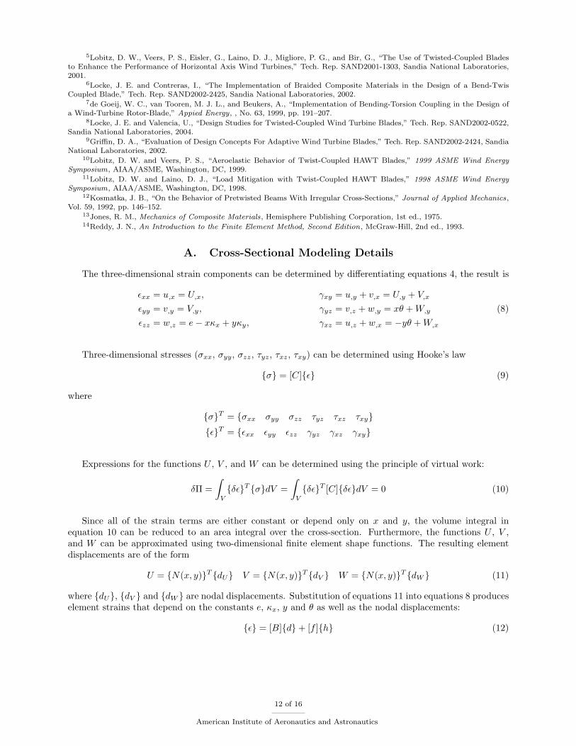
A. Cross-Sectional Modeling Details

The three-dimensional strain components can be determined by differentiating equations 4, the result is

εxx = u,x = U,x, γxy = u,y + v,x = U,y + V,x

εyy = v,y = V,y, γyz = v,z + w,y = xθ + W,y (8)εzz = w,z = e− xκx + yκy, γxz = u,z + w,x = −yθ + W,x

Three-dimensional stresses (σxx, σyy, σzz, τyz, τxz, τxy) can be determined using Hooke’s law

{σ} = [C]{ε} (9)

where

{σ}T = {σxx σyy σzz τyz τxz τxy}{ε}T = {εxx εyy εzz γyz γxz γxy}

Expressions for the functions U , V , and W can be determined using the principle of virtual work:

δΠ =∫

V

{δε}T {σ}dV =∫

V

{δε}T [C]{δε}dV = 0 (10)

Since all of the strain terms are either constant or depend only on x and y, the volume integral inequation 10 can be reduced to an area integral over the cross-section. Furthermore, the functions U , V ,and W can be approximated using two-dimensional finite element shape functions. The resulting elementdisplacements are of the form

U = {N(x, y)}T {dU} V = {N(x, y)}T {dV } W = {N(x, y)}T {dW } (11)

where {dU}, {dV } and {dW } are nodal displacements. Substitution of equations 11 into equations 8 produceselement strains that depend on the constants e, κx, y and θ as well as the nodal displacements:

{ε} = [B]{d}+ [f ]{h} (12)

12 of 16


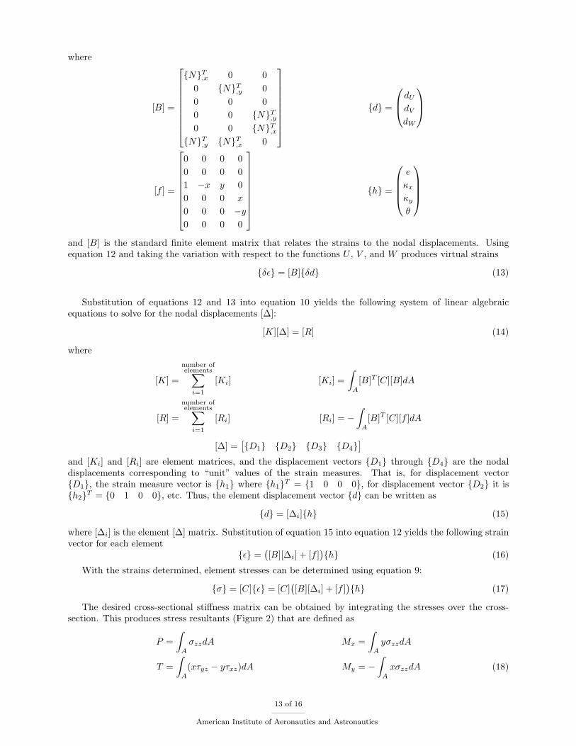
where

[B] =

{N}T,x 0 0

0 {N}T,y 0

0 0 00 0 {N}T

,y

0 0 {N}T,x

{N}T,y {N}T

,x 0

{d} =

dU

dV

dW

[f ] =

0 0 0 00 0 0 01 −x y 00 0 0 x

0 0 0 −y

0 0 0 0

{h} =

e

κx

κy

θ

and [B] is the standard finite element matrix that relates the strains to the nodal displacements. Usingequation 12 and taking the variation with respect to the functions U , V , and W produces virtual strains

{δε} = [B]{δd} (13)

Substitution of equations 12 and 13 into equation 10 yields the following system of linear algebraicequations to solve for the nodal displacements [∆]:

[K][∆] = [R] (14)

where

[K] =

number ofelements∑

i=1

[Ki] [Ki] =∫

A

[B]T [C][B]dA

[R] =


i=1

[Ri] [Ri] = −∫

A

[B]T [C][f ]dA

[∆] =[{D1} {D2} {D3} {D4}

]and [Ki] and [Ri] are element matrices, and the displacement vectors {D1} through {D4} are the nodaldisplacements corresponding to “unit” values of the strain measures. That is, for displacement vector{D1}, the strain measure vector is {h1} where {h1}T = {1 0 0 0}, for displacement vector {D2} it is{h2}T = {0 1 0 0}, etc. Thus, the element displacement vector {d} can be written as

{d} = [∆i]{h} (15)

where [∆i] is the element [∆] matrix. Substitution of equation 15 into equation 12 yields the following strainvector for each element

{ε} =([B][∆i] + [f ]

){h} (16)

With the strains determined, element stresses can be determined using equation 9:

{σ} = [C]{ε} = [C]([B][∆i] + [f ]

){h} (17)

The desired cross-sectional stiffness matrix can be obtained by integrating the stresses over the cross-section. This produces stress resultants (Figure 2) that are defined as

P =∫

A

σzzdA Mx =∫

A

yσzzdA

T =∫

A

(xτyz − yτxz)dA My = −∫

A

xσzzdA (18)

13 of 16


For each element, these stress resultants can be written in matrix form as

{Fi} =∫

A

[f ]T {σ}dA =(∫

A

[f ]T [C][B]dA[∆i] +∫

A

[f ]T [C][f ]dA

){h} (19)

where{Fi}T = {P My Mx T}i

Summing over all of the elements produces the result

{FE} = [D]{h} (20)

where

[D] = [D1]− [R]T [δ] (21)

[D1] =


i=1

∫A

[f ]T [C][f ]dA

−[R]T [δ] =


i=1

∫A

[f ]T [C][B]dA[δi] (22)

{FE}T = {F}T = {P My Mx T}

[D] is the desired cross-sectional stiffness matrix, and the subscript“E” denotes forces due to elasticdeformation

A.A. Element Coordinate System

All stress-strain relations are based on orthotropic material properties for each layer of material. Theseproperties are specified in the material 1, 2, 3 coordinate system shown in Figure 8. The transformationfrom material 1, 2, 3 coordinates to global x, y, z coordinates consists of two steps. First, the transformationis determined between material 1, 2, 3 coordinates and element x, y, z coordinates. The material 1, 2 axesare obtained by rotating the element x, y axes through an angle θ about the z axis as shown in Figure 8.Note that the material 3 axis coincides with the element z axis. The second transformation is betweenelement x, y, z coordinates and global x, y, z coordinates. The element y, z axes are obtained by rotatingthe global x, y axes through an angle α about the z axis as shown in Figure 9. Note that the element x axiscoincides with the global z axis. In general, the angle α will vary within an element and must be determinedby evaluating the Jacobian matrix.

Figure 8. Beam cross-section material and element coordinate systems.

A.B. Element Shape Functions

Rectangular Lagrange quadratic elements,14 Figure 10, were chosen for the current cross-sectional modelingapproach. These elements are used to interpolate the element displacements and the cross-sectional geometry.The element shape functions are given in equation 23.

14 of 16


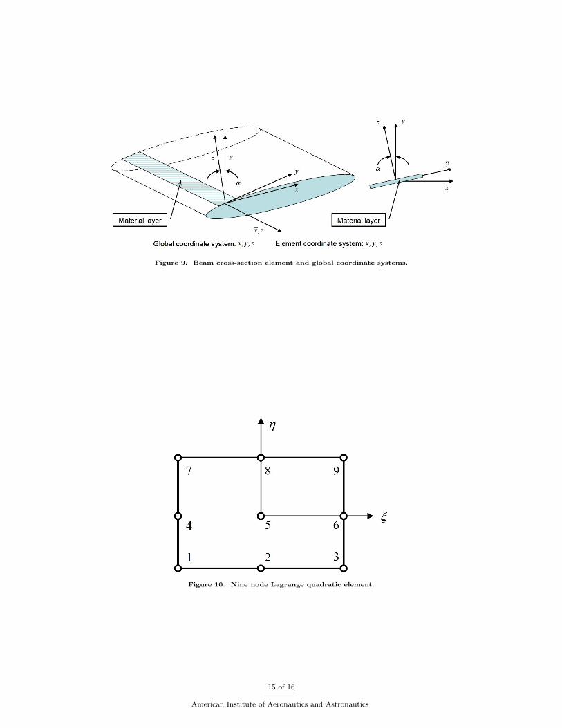
Figure 9. Beam cross-section element and global coordinate systems.

Figure 10. Nine node Lagrange quadratic element.

15 of 16


N1 = 14 (ξ

2 − ξ)(η2 − η) N2 = 12 (1− ξ2)(η2 − η) N3 = 1

4 (ξ2 + ξ)(η2 − η)

N4 = 12 (ξ

2 − ξ)(1− η2) N5 = (1− ξ2)(1− η2) N6 = 12 (ξ

2 + ξ)(1− η2)

N7 = 14 (ξ

2 − ξ)(η2 + η) N8 = 12 (1− ξ2)(η2 + η) N9 = 1

4 (ξ2 + ξ)(η2 + η) (23)

The cross-section is modeled based on defining the element ξ coordinate in the positive s direction as shownin Figure 11.

Figure 11. Positive s direction for element coordinate.

16 of 16


laminate design for coupled wind turbine blades

Documents