A brief survey of the LAMMPS MD code:intro, case studies, and future development

Paul Crozier, Steve Plimpton, Aidan Thompson, Mike Brown

February 24, 2010

LAMMPS Users’ Workshop

CSRI Building, Albuquerque, NM

Sandia is a multiprogram laboratory operated by Sandia Corporation, a Lockheed Martin Company,for the United States Department of Energy under contract DE-AC04-94AL85000.

• MD: molecular dynamics• F = ma• Classical dynamics• Rapidly grown in popularity and use in research• Computationally intensive, especially computation of

nonbonded interactions• Uses force fields: mathematical models of interatomic

interactions

A brief introduction to MD

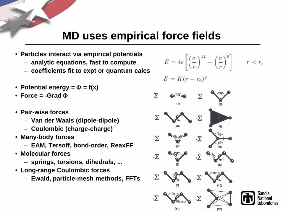
MD uses empirical force fields• Particles interact via empirical potentials

– analytic equations, fast to compute– coefficients fit to expt or quantum calcs

• Potential energy = Φ = f(x)• Force = -Grad Φ

• Pair-wise forces– Van der Waals (dipole-dipole)– Coulombic (charge-charge)

• Many-body forces– EAM, Tersoff, bond-order, ReaxFF

• Molecular forces– springs, torsions, dihedrals, ...

• Long-range Coulombic forces– Ewald, particle-mesh methods, FFTs

MD in the Middle

• Quantum mechanics– electronic degrees of freedom, chemical reactions– Schrodinger equation, wave functions– sub-femtosecond timestep, 1000s of atoms, O(N3)

• Atomistic models– molecular dynamics (MD), Monte Carlo (MC)– point particles, empirical forces, Newton's equations– femtosecond timestep, millions of atoms, O(N)

• Mesoscale to Continuum– finite elements or finite difference on grids– coarse-grain particles: DPD, PeriDynamics, ...– PDEs, Navier-Stokes, stress-strain– microseconds seconds, microns meters, O(N3/2)

Distance

Tim

e

Å m

10-1

5 s

year

s

QMMD

MESO

FEADesign

Algorithmic Issues in MD

• Speed– parallel implementation

• Accuracy– long-range Coulombics

• Time scale– slow versus fast degrees of freedom

• Length scale– coarse-graining

Classical MD in Parallel

• MD is inherently parallel– forces on each atom can be computed simultaneously– X and V can be updated simultaneously

• Most MD codes are parallel– via distributed-memory message-passing paradigm (MPI)

• Computation scales as N = number of atoms– ideally would scale as N/P in parallel

• Can distribute:– atoms communication = scales as N– forces communication = scales as N/sqrt(P)– space communication = scales as N/P or (N/P)2/3

Parallelism via Spatial-Decomposition• Physical domain divided into 3d boxes, one per processor• Each proc computes forces on atoms in its box

using info from nearby procs• Atoms "carry along" molecular topology

as they migrate to new procs• Communication via

nearest-neighbor 6-way stencil

• Optimal scaling for MD: N/Pso long as load-balanced

• Computation scales as N/P• Communication scales

sub-linear as (N/P)2/3

(for large problems)• Memory scales as N/P

A brief introduction to LAMMPS

• Massively parallel, general purpose particle simulation code.• Developed at Sandia National Laboratories, with

contributions from many labs throughout the world.• Over 170,000 lines of code.• 14 major releases since September 2004• Continual (many times per week) releases of patches (bug

fixes and patches)• Freely available for download under GPL

lammps.sandia.govTens of thousands of downloads since September 2004Open source, easy to understand C++ codeEasily extensible

LAMMPS: Large-scale Atomic/Molecular Massively Parallel Simulator

How to download, install, and use LAMMPS

• Download page:lammps.sandia.gov/download.html

• Installation instructions:lammps.sandia.gov/doc/Section_start.htmlgo to lammps/srctype “make your_system_type”

• To perform a simulation:lmp < my_script.in

How to get help with LAMMPS

1. Excellent User’s Manual:http://lammps.sandia.gov/doc/Manual.htmlhttp://lammps.sandia.gov/doc/Section_commands.html#3_5

2. Search the web: can include “lammps-users” as a search keyword to search old e-mail archives

3. Try the wiki: http://lammps.wetpaint.com/

4. Send e-mail to the user’s e-mail list:http://lammps.sandia.gov/mail.html

5. Contact LAMMPS developers: http://lammps.sandia.gov/authors.htmlSteve Plimpton, sjplimp@sandia.govAidan Thompson, athomps@sandia.govMike Brown, wmbrown@sandia.govPaul Crozier, pscrozi@sandia.gov

Force fields available in LAMMPS

• Biomolecules: CHARMM, AMBER, OPLS, COMPASS (class 2),long-range Coulombics via PPPM, point dipoles, ...

• Polymers: all-atom, united-atom, coarse-grain (bead-spring FENE),bond-breaking, …

• Materials: EAM and MEAM for metals, Buckingham, Morse, Yukawa,Stillinger-Weber, Tersoff, AI-REBO, Reaxx FF, ...

• Mesoscale: granular, DPD, Gay-Berne, colloidal, peri-dynamics, DSMC ...

• Hybrid: can use combinations of potentials for hybrid systems:water on metal, polymers/semiconductor interface,colloids in solution, …

Easily add your own LAMMPS feature

• New user or new simulation always want new feature not in code

• Goal: make it as easy as possible for us and others to add new featurescalled “styles” in LAMMPS:particle type, pair or bond potential, scalar or per-atom computation"fix": BC, force constraint, time integration, diagnostic, ...input command: create_atoms, set, run, temper, ...over 75% of current 170K+ lines of LAMMPS is add-on styles

• Enabled by C++"virtual" parent class for all pair potentialsdefines interface: compute(), coeff(), restart(), ...add feature: add 2 lines to header file, add files to src dir, re-compilefeature won't exist if not used, won't conflict with rest of code

• Of course, someone has to write the code for the feature!

LAMMPS’s parallel performance• Fixed-size (32K atoms) and scaled-size (32K atoms/proc)

parallel efficiencies• Metallic solid with EAM potential

• Billions of atoms on 64K procs of Blue Gene or Red Storm• Opteron processor speed: 5.7E-6 sec/atom/step (0.5x for LJ,

12x for protein)

Particle-mesh Methods for Coulombics• Coulomb interactions fall off as 1/r so require long-range for accuracy

• Particle-mesh methods:partition into short-range and long-range contributionsshort-range via direct pairwise interactionslong-range:

interpolate atomic charge to 3d meshsolve Poisson's equation on mesh (4 FFTs)interpolate E-fields back to atoms

• FFTs scale as NlogN if cutoff is held fixed

Parallel FFTs• 3d FFT is 3 sets of 1d FFTs

in parallel, 3d grid is distributed across procsperform 1d FFTs on-processor

native library or FFTW (www.fftw.org)1d FFTs, transpose, 1d FFTs, transpose, ...

"transpose” = data transfertransfer of entire grid is costly

• FFTs for PPPM can scale poorlyon large # of procs and on clusters

• Good news: Cost of PPPM is only ~2x more than 8-10 Angstrom cutoff

Time Scale of Molecular Dynamics

• Limited timescale is most serious drawback of MD

• Timestep size limited by atomic oscillations:– C-H bond = 10 fmsec ½ to 1 fmsec timestep– Debye frequency = 1013 2 fmsec timestep

• A state-of-the-art “long” simulation is nanoseconds toa microsecond of real time

• Reality is usually on a much longer timescale:– protein folding (msec to seconds)– polymer entanglement (msec and up)– glass relaxation (seconds to decades)

Extending Timescale• SHAKE = bond-angle constraints, freeze fast DOF

– up to 2-3 fmsec timestep– rigid water, all C-H bonds– extra work to enforce constraints

• rRESPA = hierarchical time stepping, sub-cycle on fast DOF– inner loop on bonds (0.5 fmsec)– next loop on angle, torsions (3-4 body forces)– next loop on short-range LJ and Coulombic– outer loop on long-range Coulombic (4 fmsec)

• Rigid body time integration via quaternions– treat groups of atom as rigid bodies (portions of polymer or protein)– 3N DOF 6 DOF– save computation of internal forces, longer timestep

Length Scale of Molecular Dynamics• Limited length scale is 2nd most serious

drawback of MD coarse-graining• All-atom:

∆t = 0.5-1.0 fmsec for C-HC-C distance = 1.5 Angscutoff = 10 Angs

• United-atom:# of interactions is 9x less∆t = 1.0-2.0 fmsec for C-Ccutoff = 10 Angs20-30x savings over all-atom

• Bead-Spring:2-3 C per bead∆t fmsec mapping is T-dependent21/6 σ cutoff 8x in interactionscan be considerable savings over united-atom

Atomistic Scale Models with LAMMPS

• Interfaces in melting solids• Adhesion properties of polymers• Shear response in metals• Tensile pull on nanowires• Surface growth on mismatched lattice• Shock-induced phase transformations• Silica nanopores for water desalination• Coated nanoparticles in solution and at interfaces• Self-assembly (2d micelles and 3d lipid bilayers)• Rhodopsin protein isomerization

Melt Interface in NiAl

• Mark Asta (UC Davis) and Jeff Hoyt (Sandia)• Careful thermostatting and equilibration of alloy system• Track motion and structure of melt interface

Polymer Adhesive Properties

• Mark Stevens and Gary Grest (Sandia)• Bead/spring polymer model, allow for bond breaking

Shear Response of Cu Bicrystal• David McDowell group (GA Tech)• Defect formation, stress relaxation, energetics of boundary region

Coated Nanoparticles at Interfaces• Matt Lane, Gary Grest (Sandia)• S sites on Au nanoparticle, alkane-thiol chains,

methyl-terminated, 3 ns sim

water decane

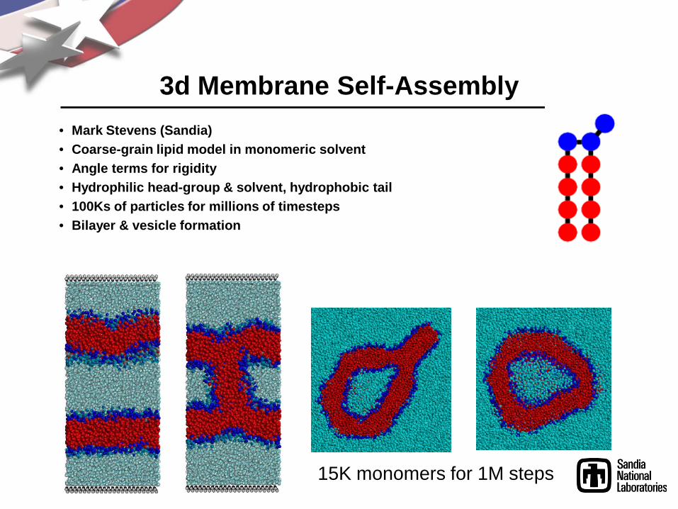
3d Membrane Self-Assembly• Mark Stevens (Sandia)• Coarse-grain lipid model in monomeric solvent• Angle terms for rigidity• Hydrophilic head-group & solvent, hydrophobic tail• 100Ks of particles for millions of timesteps• Bilayer & vesicle formation

15K monomers for 1M steps

Membrane Fusion

• Gently push together ...

Aspherical Nanoparticles• Mike Brown (Sandia)• Ellipsoidal particles interacting via Gay-Berne potentials

(LC), LJ solvent• Nanodroplet formation in certain regimes of phase space

Rigid Nanoparticle Self-Assembly

(Sharon Glotzer et al., Nano Letters, 3, 1341 (2003).

• Multiple rigid bodies• Quaternion integration• Brownian dynamics• Self-assembly phases

LAMMPS’s Reactive Force Fields Capability

Why Reactive Force Fields?• Material behavior often dominated by chemical processes• HE, Complex Solids, Polymer Aging• Quantum methods limited to hundreds of atoms• Ordinary classical force fields limited accuracy• We need to have the best of both worlds ⇒Reactive force fields Why build Reactive Force Fields into LAMMPS?• Reactive force fields typically exist as custom serial MD codes • LAMMPS is a general parallel MD code

LAMMPS+ReaxFF enables direct simulation of detailed initial energy propagation in HE

–Improved understanding of sensitivity will aid development of more reliable microenergetic components

–Goal: Identify the specific atomistic processes that cause orientation-dependent detonation sensitivity in PETN

–Thermal excitation simulations used as proof-of-concept

–Collaborating with parallel DoD-funded effort at Caltech (Bill Goddard, Sergey Zybin)

–Now running multi-million atom shock-initiated simulations with different orientations

–Contracted Grant Smith to extend his HMX/RDX non-reactive force field to PETN

Propagation of reaction front due to thermal excitation of a thin layer at the center of the sample for 10 picoseconds. Top: atoms colored by potential energy. Bottom: atoms colored by temperature (atoms below 1000K are not shown).

Complex molecular structure of unreacted tetragonal PETN crystal, C (gray), N (blue), O (red), and H (white).

MD Simulation of Shock-induced Structural Phase Transformation in Cadmium Selenide

a-direction: 3-Wave Structure: tetragonal region forms between elastic wave and rocksalt phase

[1000]

[0110]

[1000]

[0001]

c-direction: 2-Wave Structure: rocksalt emerges directly from elastically compressed material

Non-equilibrium MD simulations of brackish water flow through silica and titania nanopores

r

z

• Water is tightly bound to hydrophilic TiO2surface, greatly hampering mobility within 5 Å of the surface.

• Simulations show that amorphous nanopores of diameter at least 14 Å can conduct water as well as Na+ and Cl- ions.

• No evidence of selectivity that allows water passage and precludes ion passage ---functional groups on pore interior may be able to achieve this.

• Small flow field successfully induces steady state solvent flow through amorphous SiO2and TiO2 nanopores in NEMD simulations.

• Complex model systems built through a detailed processs involving melting, quenching, annealing, pore drilling, defect capping, and equilibration.

• 10-ns simulations carried out for a variety of pore diameters for for both SiO2 and TiO2nanopores.

• Densities, diffusivities, and flows of the various species computed spatially, temporally, and as a function of pore diameter.

Water flux through an 18 Å TiO2 nanopore.

Spatial map of water diffusivities in a 26 Å TiO2 nanopore.

Rhodopsin photoisomerization simulation

• 190 ns simulation– 40 ns in dark-adapted state (J. Mol. Biol., 333, 493, (2003))– 150 ns after photoisomerization

• CHARMM force field• P3M full electrostatics• Parallel on ~40 processors; more than 1 ns simulation / day of real time• Shake, 2 fs time step, velocity Verlet integrator• Constant membrane surface area• System description

– All atom representation– 99 DOPC lipids– 7441 TIP3P waters– 348 rhodopsin residues– 41,623 total atoms– Lx=55 Å, Ly=77 Å, Lz=94-98 Å

Photoisomerization of retinal

40-ns simulation in dark-adapted state

Isomerization occurs within 200 fs.

NH

32

165

4

1617

18

78

9

19

10

1112

1314

15 20ε

δγ

βα

11-cis retinal

NH

32

1654

1617

18

78

9

19

10

1112

1314

15 20ε

δγβ

α"all-trans" retinal

Dihedral remains in trans during subsequent 150 ns of relaxation

Transition in retinal’s interaction environment

Retinal’s interaction with the rest of the rhodopsin molecule weakens and is partially compensated by a stronger solvent interaction

Most of the shift is caused by breaking of the salt bridge between Glu 113 and the PSB

Whole vesicle simulation

• Enormous challenge due to sheer size of the system5 million atoms prior to filling box with waterEstimate > 100 million atoms total

• Sphere of tris built using Cubit software, then triangular patches of DOPC lipid bilayers were cut and placed on sphere surface.

Radiation damage simulations

► Radiation damage is directly relevant to several nuclear energy applications

Reactor core materials Fuels and cladding Waste forms

► Experiments are not able to elucidate the mechanism involved in structural disorder following irradiation

► Classical simulations can help provide atomistic detail for relaxation processes involved

► Electronic effects have been successfully used in cascade simulations of metallic systems

MD model for radiation damage simulations

►Gadolinium pyrochlore waste form (Gd2Zr2O7)►Natural pyrochlores are stable over geologic times and shown

to be resistant to irradiation (Lumpkin, Elements 2006).►Recent simulations (without electronic effects) exist for

comparison (Todorov et al, J. Phys. Condens. Matter 2006).

10.8 Å 162 Å

1 unit cell, 88 atoms 15 x 15 x 15 supercell, 297k atoms(only Gd atoms shown)

Defect analysis

► How the defect analysis works:1. Shape matching algorithm was used.*2. Nearest neighbors defined as those

atoms in the first RDF peak.3. Clusters formed by each Gd atom and its

nearest Gd neighbors are compared with clusters formed by those neighbors and their nearest Gd neighbors.

4. If the cluster shapes match, the atom is considered “crystalline”; otherwise, it is considered “amorphous.”

► Why only Gd atoms were used:1. RDF analysis produces clear picture of

crystal structure.2. Clearly shows the cascade damage.

* Auer and Frenkel, J. Chem. Phys. 2004Ten et al, J. Chem. Phys. 1996

Results of defect analysis

0

50

100

150

200

250

300

350

400

450

500

0.01 0.1 1 10 100

Time / ps

Def

ecti

ve G

d

tau_p = 200 fs

no TTMγp = 0.277 g/(mol fs)γp = 1.39 g/(mol fs)γp = 2.77 g/(mol fs)

Future areas of LAMMPS development

• Alleviations of time-scale and spatial-scale limitations• Improved force fields for better molecular physics• New features for the convenience of users

LAMMPS development areas

Timescale & spatial scale Force fields Features

Faster MD

Accelerated MD

FF parameter data base

Multiscale simulation

Coarse graining

On a single processor

In parallel, or with load balancing

Temperature accelerated dynamics

Parallel replica dynamics

Forward flux sampling

Aggregation

Rigidification

Couple to quantum

Couple to fluid solvers

Couple to KMC

Auto generation

novel architectures, or N/P < 1

Biological & organics

Informatics traj analysis

Solid materials

NPT for non-orthogonal boxes

Chemical reactions

ReaxFF

Bond making/swapping/breaking

Functional forms

Charge equilibration

Long-range dipole-dipole interactions

Allow user-defined FF formulas

Electrons & plasmas

Aspherical particles

User-requested features

Peridynamics