landscape connectivity: a conservation application of ...bdeyoung/connectivity/bunn_et_al.pdf ·...

Journal of Environmental Management (2000) 59, 265–278doi:10.1006/jema.2000.0373, available online at http://www.idealibrary.com on

Landscape connectivity: A conservationapplication of graph theory

A. G. Bunn†§*, D. L. Urban† and T. H. Keitt‡

We use focal-species analysis to apply a graph-theoretic approach to landscape connectivity in the CoastalPlain of North Carolina. In doing so we demonstrate the utility of a mathematical graph as an ecologicalconstruct with respect to habitat connectivity. Graph theory is a well established mainstay of informationtechnology and is concerned with highly efficient network flow. It employs fast algorithms and compactdata structures that are easily adapted to landscape-level focal species analysis. American mink (Mustelavison) and prothonotary warblers (Protonotaria citrea) share the same habitat but have different dispersalcapabilities, and therefore provide interesting comparisons on connections in the landscape. We built graphsusing GIS coverages to define habitat patches and determined the functional distance between the patcheswith least-cost path modeling. Using graph operations concerned with edge and node removal we foundthat the landscape is fundamentally connected for mink and fundamentally unconnected for prothonotarywarblers. The advantage of a graph-theoretic approach over other modeling techniques is that it is a heuristicframework which can be applied with very little data and improved from the initial results. We demonstrate theuse of graph theory in a metapopulation context, and suggest that graph theory as applied to conservationbiology can provide leverage on applications concerned with landscape connectivity. 2000 Academic Press

Keywords: landscape ecology, graph theory, connectivity, modeling, metapopulations, focalspecies, American mink, Mustela vison, prothonotary warblers, Protonotaria citrea.

Introduction

The current trend in ecological research andland management is to focus on large biogeo-graphic areas, which leaves the researcherand manager searching for landscape-scaledata (Christensen et al., 1996; Noss, 1996).Indeed, the interpretation of large spatialdata, conceptually and technologically, canbe the limiting factor in making conservationbiology and ecosystem management a tan-gible goal. Because the internal heterogene-ity of landscapes makes habitat-conservationplanning a formidable challenge, modelingthe spatial aspects of landscapes is a crit-ical key to understanding. Until now, thevaried approaches to building these mod-els have focused primarily on two types ofspatial data, coverages of vectors (polygons)or raster grids. We demonstrate the utilityof a less familiar type of lattice, the graph(Harary, 1969), in determining landscapeconnectivity using focal-species analysis in

ŁCorresponding author

† Nicholas School of theEnvironment, DukeUniversity, Durham, NC27708, USA

‡ National Center forEcological Analysis andSynthesis, Santa Barbara,CA 93101, USA

§ Present address:Mountain ResearchCenter, Montana StateUniversity, Bozeman, MT59717, USA

Received 31 May 2000;accepted 30 June 2000

an island model. A graph represents a binarylandscape of habitat and non-habitat, wherepatches are described as nodes and the con-nections between them as edges.

Graph theory is a widely applied frame-work in geography, information technol-ogy and computer science. It is primarilyconcerned with maximally efficient flowor connectivity in networks (Gross andYellen, 1999). To this end, graph-theoreticapproaches can provide powerful leverageon ecological processes concerned with con-nectivity as defined by dispersal. In partic-ular, graph theory has great potential foruse in applications in a metapopulation con-text. Urban and Keitt (2000) have introducedlandscape-level graph-theory to ecologists,and here we build on that work by exam-ining habitat connectivity for two speciesthat share the same habitat but have dif-ferent dispersal capabilities. Specifically, weask how American mink (Mustela vison) andprothonotary warblers (Protonotaria citrea)

0301–4797/00/080265C14 $35.00/0 2000 Academic Press

266 A. G. Bunn et al.

perceive the same landscape. We explore thesensitivity of landscape connectivity throughgraph operations concerned with edge defini-tion. We also examine each habitat patch’srole in maintaining landscape connectiv-ity in terms of source strength (Pulliam,1988) and long-distance traversability (denBoer, 1968; Levins, 1969) using graph oper-ations concerned with node removal. Thistype of analysis is done very efficientlywith graph theory. We also present anecologically appealing way to calculate thefunctional distance between habitat patchesusing least-cost path modeling. Graph the-ory as applied to landscapes represents animportant advance in spatially explicit mod-eling techniques because it is an additiveframework: analysis of a simple, preliminarygraph can prioritize further data collection toimprove the graph model.

Study area and methods

Study area

Our study focuses on the Alligator RiverNational Wildlife Refuge (NWR) and sur-rounding counties on the Coastal Plain ofNorth Carolina (35°500N; 75°550W). It is ariverine and estuarine ecosystem with anarea of almost 580 000 ha and over 1400 kmof shoreline. The area is rich in wildlife habi-tat, dominated by the Alligator River NWR,the Pocosin Lakes NWR, Lake Mattamus-keet NWR, Swanquarter NWR, and a varietyof other federal, state, and private wildlands(Figure 1).

The vegetation is characterized by theSouthern Mixed Hardwoods forest commu-nity. The area has many diverse vegetationtypes, including fresh water swamps, pinewoods and coastal vegetation. In the uplandcommunity, dominant species include manytypes of oak (Quercus spp.), American Beech(Fagus grandifolia), and evergreen magno-lia (Magnolia grandiflora). Mature standsmay have five to nine codominants. Thewet lowlands are dominated by bald cypress(Taxomodium distichum). The pine woodsare dominated by longleaf pine (Pinus palus-tris), but loblolly pine (P. taeda) and slashpine (P. elliottii) are also important (Vankat,1979).

Focal species

Because connectivity occurs at multiplescales and multiple functional levels (Noss,1991), we have chosen two focal species toapply a graph-theoretic approach to connec-tivity. Focal species analysis is an essentialtool for examining connectivity in a reallandscape, as individual species have differ-ent spatial perceptions (O’Neill et al., 1988).The American mink and the prothonotarywarbler are appropriate candidates for focalspecies analysis as they share very similarhabitat but have different ecological require-ments, and fall into different categories asfocal species. Both species are wetland depen-dent and indicators of wetland quality andabundance in a landscape. Both are charis-matic. Furthermore, as meso-predators minkhave small but important roles as a keystonespecies (Miller et al., 1998/1999).

American mink are meso-level, semi-aquatic carnivores that occur in riverine,lacustrine and palustrine environments(Gerell, 1970). In chief, they are nocturnaland their behavior largely depends on preyavailability. They have a great deal of vari-ation in their diet according to habitat type,season and prey availability (Dunstone andBirks, 1987). Muskrats (Odantra zibethicus)are a preferred prey item (Hamilton, 1940;Wilson, 1954), but mink diets in North Car-olina are composed of aquatic and terrestrialanimals, as well as semiaquatic elements(e.g. waterfowl; Wilson, 1954). In the south-east they have home ranges on the order of1 ha and a dispersal range of roughly 25 km(Nowak, 1999).

Prothonotary warblers are neotropical mig-rants that breed in flooded or swampy maturewoodlands. They have two very unusualtraits in common with wood warblers in thatthey are cavity nesters and prefer nest sitesover water. They are forest interior birdsthat experience heavy to severe parasitismby brown-headed cowbirds (Molothrus ater);(Petit, 1999). They are primarily insectivo-rous, occasionally feeding on fruits or seed(Curson et al., 1994). Preliminary data indi-cate that natal dispersal ranges from lessthan 1 km to greater than 12 km (Petit, 1999).Although this is formulated from a smallsample, it is on the same order as other songbird dispersal (e.g. Nice, 1933; Sutherlandet al., 2000). Here, we posit warbler dispersal

Landscape connectivity 267

Figure 1. Study area in North Carolina with major roads and streams shown along with bottomlandhardwood forest (focal species habitat) identified using GIS analysis.

to be 5 km and return to the uncertainty ofthis statement later.

Geospatial data

To our knowledge there are no currentdata on the spatial distribution of the focalspecies in our study area. The decline intrapping of the mink has perversely led to adecline in good biological information on thespecies. We are unaware of any work donewith mink in the study area since Wilson’s(1954) study. The Breeding Bird Surveyindicates that this study area contains oneof the highest concentrations of prothonotary

warblers in the Southeast (Price et al., 1995).Finer scale spatial information is not readilyavailable.

Mink and prothonotary warblers are habi-tat specialists that use the same habitat.To identify habitat patches in the land-scape we combined data from the US Fishand Wildlife Service’s National WetlandsInventory (http://wetlands.fws.gov) and a1996 land-use coverage from the NationalCenter for Geographic Information and Anal-ysis (http://www.negia.ucsb.edu). Both werederived from Landsat 7 Thematic Map-per imagery with 30-m cells. Cells thatwere defined as being bottomland hardwoodswamp or oak gum cypress swamp, and


riverine, lacustrine, or palustrine forestedwetland were selected as habitat. These cellswere then aggregated into regions usingan eight-neighbor rule, and the interven-ing matrix was described as non-habitat. Wealso used zonal averaging techniques in anattempt to account for functional scaling inthe habitat and found that the patch defini-tion was robust. Transportation and hydrog-raphy digital line graphs were obtainedfor the study area from the US Geologi-cal Survey (http://www.usgs.gov) at 1:100 000resolution.

Graph theory

Urban and Keitt (2000) give a generaldescription of ecological applications of graphtheory and readers should refer to any num-ber of excellent texts on graphs as a primer(e.g. Gross and Yellen, 1999). However, thissection describes the graph operations anddefinitions used in this study. While there arenumerous excellent texts on the formalismsof graph theory (e.g. Gross and Yellen, 1999),the following largely conforms to Harary’s(1969) classic text. A graph G is a set of nodesor vertices V.G/ and edges E.G/ such thateach edge eijDvivj connects nodes vi and vj.A path in a graph is a unique sequence ofnodes. The distance of a path from vl to vn ismeasured by the length of the unique set ofedges implicitly defined by the path. A pathis closed if nlDvn. Three or more nodes in aclosed path is called a cycle. A path with nocycles is a tree. A tree that includes all thevertices in the graph is a spanning tree. Theminimum spanning tree is the spanning treein the graph with the shortest total length.The minimum spanning tree in effect repre-sents the parsimoniously connected backboneof the graph.

A graph is connected if a path existsbetween each pair of nodes. An unconnectedgraph may include several connected com-ponents or subgraphs. A graph’s diameter,d.G/, is the longest path between any twonodes in the graph, where the path lengthbetween those nodes is itself the shortest pos-sible length. If nodes i and j are not adjacent,then the shortest path between them cannotbe the distance between them but must usestepping-stones. Here, we use graph diam-eter (or diameter of the largest component)

as an index to overall traversability of thehabitat mosaic.

A graph is defined by two data structures:one that describes its nodes and one thatdescribes its edges. We defined the nodes(habitat patches) by their spatial centroidand size (x, y, s). We defined the edges by adistance matrix D whose elements dij are thefunctional distances between patches i and j.For n patches D is n by n but because dijDdjiand diiDdjjD0, it is sufficient to compute thelower triangle of the matrix.

Although the spatial array of nodes is sim-ple to produce from a GIS, the other matricesare not as easy to define. Distance betweenpatches can be measured in several differ-ent ways: edge to edge, centroid to centroid,centroid to edge, etc. However, measuringthese as Euclidean distance makes littlesense when the variance in mortality costassociated with traversal of the interveninghabitats is large, and cost associated withtraversal of the intervening habitats is largeand spatially heterogeneous. Few organismsor even ecosystem processes, such as ground-water movement or wildfire spread, move inthis way. To differing extents they are allconstrained by the landscape. Good multi-dimensional models exist to predict someecosystem processes (e.g. pollution plumes;Bear and Verruit, 1987) but not others. Spa-tially explicit models that simulate the dis-persal of animals have been explored in somedepth but the process is still poorly under-stood (Gaines and Bertness, 1993). Most arecomplex parametric models which are data-hungry. They require specific informationand are hard to parameterize (Gustafson andGardner, 1996).

For this reason, we have computed D not asEuclidean distances but as a series of least-cost paths on a cost surface appropriate tothe organisms in question. These paths aredesigned to approximate the actual distancethe focal species (or any other landscapeagent, e.g. fire) covers moving from one patchto the next. For instance, in this riverineecosystem, the path a mink might take fromone side of a river delta to the other wouldlikely involve traversing the shore for 10 kmunder cover, rather than a 5-km swim acrossopen water. This allows the animal to usestepping-stones of other habitat (low cost)along the way rather than set off into anunknown habitat matrix (high cost). The


least-cost modeling combines habitat qualityand Euclidean distance in determining dij.

Cost was defined in 90-m cells (aggre-gated up from 30-m cells to improve pro-cessing time) by a surface comprised of x,y and z, where z was a uniform impedancethat represented the cost of moving throughthat cell, i.e. its resistance to dispersal.Weights were approximated, based on per-ceived traversability. Cells corresponding toareas of habitat were given a weight of 0Ð5, allother forest types were given a weight of one.Cells classified as riverine/estuarine herba-ceous were given a weight of two. Shrublandwas given a weight of three. Sparsely vege-tated cells (cultivated, managed herbaceous)were given a weight of four. Areas of devel-opment and large water bodies were givena weight of five. Streams were defined with aweight of one. We used grid functions insidea macro in ArcInfo 7.2.1 (ESRI, 1998) to iter-atively loop through the array of patches andcompute dij for each unique pair of nodes inthe array. The macro uses area-weighted dis-tance functions to calculate least-cost paths.These functions are similar to Euclidean dis-tance functions, but instead of working ingeographical units they work in cost units.

We explored alternative methods for con-structing D, including Euclidean distanceand resistance-weighted distance betweennodes. We found that the topology of thegraph is robust and not sensitive to thedifference between least-cost path distanceand Euclidean distance except at the scale oflarge obstacles in the landscape. For instance,least-cost paths in our model did not cross the5-km mouth of the Alligator river when mov-ing from the eastern side of the study area butchose a route through habitat instead. In thiscase Euclidean distance and least-cost pathdistance were quite different. The least-costpath technique is useful to land managers asthe surface can be parameterized based onbest available data. Thus, the surface can betailored to features in the landscape for whichthe manager has knowledge. The surface canbe refined as data becomes available, e.g. inthe form of radio tracking.

Gustafson and Gardner (1996) found thatdispersal routes are difficult to predict in evenslightly heterogeneous landscapes. We havekept that in mind by building a simple costsurface that avoids committing the animalsto movement patterns that are not readily

possible to predict at 90-m resolution. We arenot suggesting that the organisms modeledmove purely according to least-cost paths. Weuse the framework because the distance of theleast-cost path is a better approximation ofthe actual distance covered than a straightline between patches. Our goal has been toget a better estimate of distance traveledusing least-cost and not to predict corridors.This modeling technique can be applied ina GIS, with limited spatial data, making itaccessible to land managers and conservationpractitioners. Despite these advantages, cost-surface analysis has been only occasionallyused by ecologists (Krist and Brown, 1994;Walker and Craighead, 1997), but widelyused in computer science which is concernedwith optimal route planning (e.g. McGeoch,1995; Bander and White, 1998). This type ofanalysis is also common in applications ofartificial intelligence (e.g. Xia et al., 1997).

To focus on scaling between the two focalspecies we chose to explicitly incorporate onlypatches greater than 100 ha in our analyses,as prothonotary warblers are not likely topersist in forest patches less than 100 ha(Petit, 1999). Using habitat patches greaterthan 100 ha results in 83 patches, roughly83% of the 53 392 ha of possible habitat.Because all habitat patches, regardless ofsize, are given the lowest value on the costsurface, they are implicitly included in allanalyses in that the species can traversethem easily as stepping-stones, accruingminimal cost.

We further defined edges by a dispersalprobability matrix P that expresses theprobability that an individual in patch i willdisperse at least the distance between patchi and j. We computed the elements of P asnegative exponential decay:

pijD�e.qÐdij/ .1/

where q is an extinction coefficient greaterthan 0. This way dispersal functions can beindexed by noting the tail distance corre-sponding to PD0Ð05 is � ln.0Ð05/Ðq�1. The taildistance for mink and prothonotary warblerare indexed as 25 km and 5 km, respectively.The tail distance is the distance to a selectedpoint on the flat tail of the dispersal-distancefunction. Other curves are possible and Clarket al. (1999) provide a discussion of alternatedispersal kernels.


The graphs are described most succinctlyby an adjacency matrix A in which aijD1 ifnodes i and j are connected and 0 if not. Weset aijD1 if dij�25 km for mink and dij�5 kmfor prothonotary warbler.

We can also define the graph’s edges interms of dispersal fluxes. Combining P and sallows us to compute dispersal flux from i to j:

fijD si

stotÐp0ij .2/

where si is relativized as the proportion ofthe total habitat area stot in i and p0ij is pijnormalized by the row sum of i in P. Becausedispersal flux is asymmetrical .fij 6Dfji/ whensi 6D sj we average the directions betweennodes to give area-weighted dispersal fluxwij:

wijDwjiD1�(

fijCfji

2

).3/

Subtracting from 1 allows the flux valueto have the smaller fluxes at greater dis-tances. The area-weighted dispersal fluxmatrix allows us to compute a version of aminimum spanning tree with more dispersalbiology incorporated.

Graph operations

With graph construction complete we per-formed two types of graph operations relat-ing to connectivity: edge thresholding andnode removal. Edge thresholding allows usto determine connectivity for mink andprothonotary warblers based on their taildispersal distances. It also allows us togauge the importance of variation of thetail distance. We removed edges from thegraph iteratively with a edge distancethresholded at 100 m to 50 000 m in 100 mincrements. At each iteration the num-ber of graph components, the number ofnodes in the largest component and thediameter of the largest component wererecorded.

Node removal is a way to examine therelative importance of habitat area andconnectivity in the landscape. We used noderemoval to tell us about the dynamics ofthe entire landscape under different habitat-loss scenarios. Nodes were removed from thegraph iteratively. We began with the entiregraph and removed nodes randomly (with

100 repetitions), by minimum area, and byendnodes with the smallest area (Urban andKeitt, 2000). An endnode in a graph is a leafin the spanning tree (here based on area-weighted flux) that is adjacent to only oneother node. All edges incident to the removednode were also removed. At each iteration ofthe removal process the graph was analyzedto determine the importance of the patchto the graph’s area-weighted dispersal flux(F), and traversability (T). Area-weighteddispersal flux was indexed as:

FDn∑i

n∑j,i 6Dj

pijsi .4/

where si is the size of node i and pij is fromEquation (1) above.

Traversability was indexed as the diameterof the largest component in the graph formedby the removal of the node:

TDd.G0/ .5/

where G0 is the largest component of G. Weuse F as an index of a patch’s source strength,after Pulliam (1988). We use T in the sense ofspreading-of-risk or rescue from catastrophe,after den Boer (1968) and Levins (1969).

Finally, we determined the importance ofindividual nodes to the entire landscape byassessing their individual contribution toarea-weighted dispersal and traversabilityin the graph by computing F and T forthe entire landscape, and then recomputingeach with a single node removed from thegraph. That node’s impact is the differencebetween the intact metric and the metricthat its removal elicited. Furthermore, wesought to determine the landscape’s overallsensitivity to scale by repeating this processwith edge definition thresholds from 2Ð5 kmto 25 km, increasing in 2Ð5-km increments.We assessed the robustness of the patches’sensitivity rankings on F and T with Spear-man’s rank correlation, using the middleedge distance of 12Ð5 km to as the referencecase.

Results

The mean distance between patches in the83ð83 matrix is 62Ð7 km. The study area andhabitat patches are illustrated in Figure 1.


0 50

80

Threshold distance (km)

Nu

mbe

r of

gra

ph c

ompo

nen

ts/G

raph

ord

er

10

20

30

40

50

60

70

5 10 15 20 25 30 35 40 45

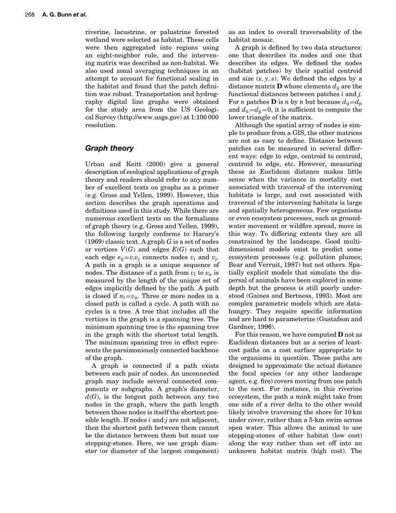
Figure 2. Number of graph components ( )and graph order ( ) as a function of effectiveedge distance.

Edge thresholding

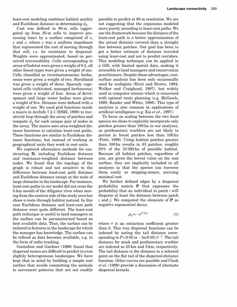
The graph begins to disconnect and frag-ment into subgraphs at a 19 km edge dis-tance, and quickly fragments into numerouscomponents containing only a few nodes(Figure 2). The diameter of the largestcomponent increases quickly with thresholddistance, peaking at 20 km and declining

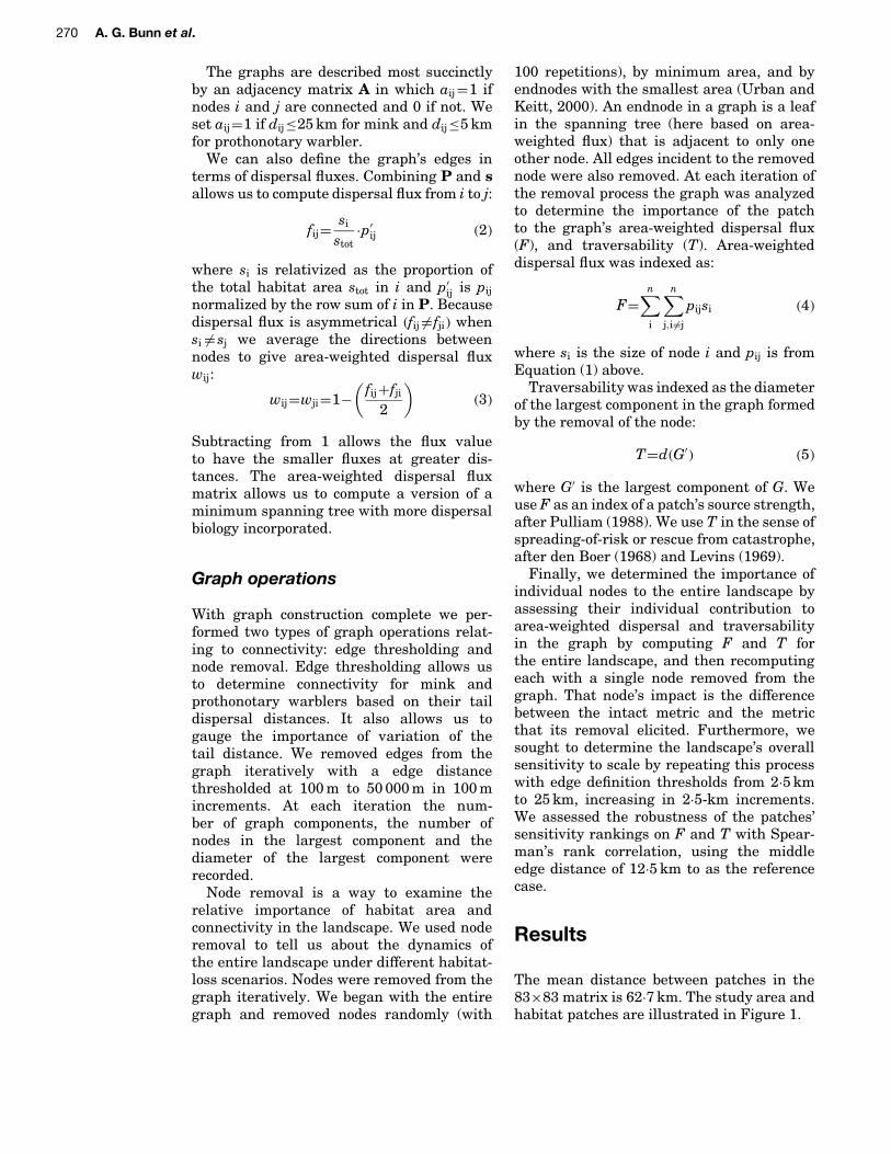
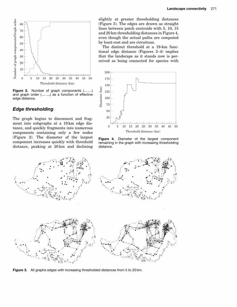
slightly at greater thresholding distances(Figure 3). The edges are drawn as straightlines between patch centroids with 5, 10, 15and 20 km thresholding distances in Figure 4,even though the actual paths are computedby least-cost and are circuitous.

The distinct threshold at a 19-km func-tional edge distance (Figures 2–4) impliesthat the landscape as it stands now is per-ceived as being connected for species with

0 50

200

Threshold distance (km)

Dia

met

er (

km)

25

50

75

100

125

150

175

5 10 15 20 25 30 35 40 45

Figure 4. Diameter of the largest componentremaining in the graph with increasing thresholdingdistance.

Figure 3. All graphs edges with increasing thresholded distances from 5 to 20 km.


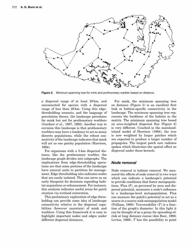
Figure 5. Minimum spanning tree for mink and prothonotary warbler based on distance.

a dispersal range of at least 20 km, andunconnected for species with a dispersalrange of less than 20 km. Using this edge-thresholding scenario, and the language ofpercolation theory, the landscape percolatesfor mink but not for prothonotary warblers(Gardner et al., 1987, 1992). Another way toenvision this landscape is that prothonotarywarblers may have a tendency to act as manydiscrete populations, while the robust con-nectivity of the landscape indicates that minkwill act as one patchy population (Harrison,1994).

For organisms with a 5-km dispersal dis-tance, like the prothonotary warbler, thelandscape graph divides into subgraphs. Theimplications from edge-thresholding opera-tions are that some portions of the landscapehave natural units to partition for manage-ment. Edge thresholding also indicates nodesthat are easily isolated. This can serve as anearly blueprint for decisions regarding habi-tat acquisition or enhancement. For instance,this analysis indicates useful areas for patchcreation via wetland restoration.

This preliminary exploration of edge thres-holding can provide some idea of landscapeconnectivity relative to the dispersal capa-bilities (however uncertain) of mink andwarblers. Using this framework it is easy tohighlight important nodes and edges underdifferent dispersal distances.

For mink, the minimum spanning treeon distance (Figure 5) is an excellent firstlook at habitat-specific connectivity in thelandscape. The minimum spanning tree rep-resents the backbone of the habitat in thematrix. The minimum spanning tree basedon area-weighted dispersal flux (Figure 6)is very different. Couched in the mainland-island model of Harrison (1994), the treeis now weighted by larger patches whichare expected to produce a larger number ofpropagules. The largest patch now radiatesspokes which illustrates the spatial effect ondispersal under these kernels.

Node removal

Node removal is habitat removal. We mea-sured the effects of node removal in two wayswhich can indicate a landscape’s potentialto provide conditions that foster metapopula-tions. Flux (F), as governed by area and dis-persal potential, measures a node’s influenceto a landscape-level metapopulation. Fluxcan measure the patch’s potential to act as asource in a source-sink metapopulation model(Pulliam, 1988). Traversability (T) is a func-tion of the graph’s diameter. In this light itcan be thought of as a proxy for spreading-of-risk or long distance rescue (den Boer, 1968;Levins, 1969). T has the possibility to point


Figure 6. Area-weighted minimum spanning tree for mink with 25-km tail dispersal.

0 80

8

Number of nodes removed

Tot

al f

lux

2

4

6

20 40 60

Figure 7. Area-weighted dispersal flux (F) as afunction of three different node pruning scenarios.( ), random; ( ), minnode; ( ), endnode.Graph defined with 25 km adjancency threshold.

out important stepping-stone patches in thelandscape. Source strength and long-distancerescue are well established in conservationbiology. F and T are codified versions of thosethat fit into the graph context.

The different node removal scenarios givedifferent pictures of the landscape. The betterperformance of endnode pruning over randomor minimum area pruning for F indicates thetendency for endnodes to be less connectedto the landscape (Figure 7). The advantageof endnode pruning is clear in its effect on T

0 80

25 000

Number of nodes removed

Dia

met

er (

m)

5000

10 000

15 000

20 40 60

20 000

Figure 8. Traversability (T ) of the largest graphcomponent as a function of three different nodeprunning scenarios. ( ), random; ( ), minnode;( ), endnode. Graph defined with 5 km adjancencythreshold.

in the graph (Figure 8). Traversability of thegraph is maintained with a majority of thegraph nodes removed. The effect of endnodepruning on this landscape may indicate thatthis riverine ecosystem has a high degree ofnatural connectivity that an ecosystem notcomprised of linearly connected features maynot posses.

Area-weighted dispersal flux relies on Pand s and is functionally similar for minkand prothonotary warblers under random,endnode, and minimum area pruning. Thethree thinning procedures produce similarresults, although endnode pruning resulted


in slightly higher flux values (Figure 7). Theeffect of different types of patch removalon traversability is markedly different formink and prothonotary warblers. For mink,with a 25-km functional adjacency thresh-old, the three removal methods produce verysimilar results. For prothonotary warblers,with 5 km functional adjacency threshold,the random and minimum area pruning pro-duce similar linear results but the effectof endnode pruning is substantially dif-ferent. Traversability of the graph is noteffected until ¾75% of the nodes are removed(Figure 8).

Node sensitivity

The spatial arrangement of habitat patchesin a landscape in combination with scalecan influence measures of connectivity (Keittet al., 1997). Our two main metrics for con-nectivity, F and T, show differing responsesto scale. Traversability, T, is indexed inde-pendently of patch area and is quite scale-dependent, showing little to no rank correla-tion between scales (Figure 9). Conversely,F is calculated explicitly with patch areaand is very robust across scales. This islikely to be a function of patch area, andilluminates interesting management and eco-logical aspects of the landscape. In a Levinsmetapopulation model, T is analogous tospreading-of-risk and is sensitive to scale.

–0.525

1.5

Effective edge distance (km)

Ran

k co

rrel

atio

n

2.5

–0.25

0

0.25

0.5

0.75

1

1.25

5 7.5 10 12.5 15 17.5 20 22.5

Figure 9. Correlation length of the vectors forarea-weighted dispersal (F; -- --) and traversability(T; ) at varying scales. Reference variables arerespective vectors at 12Ð5 km edge distance. Filledsymbols are significant at P<0Ð005.

In the more commonly used Pulliam model,F is analogous to source-sink strength and isnot sensitive to scale because it is influencedmost by close patches (short distance).

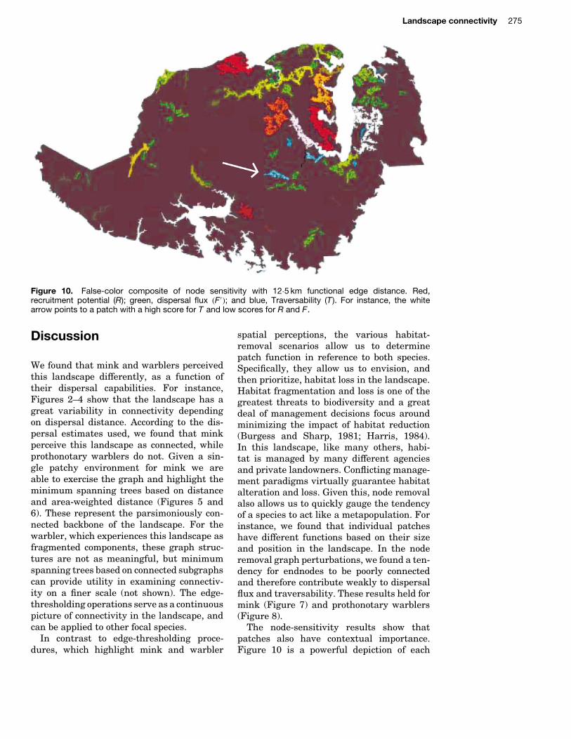
We have chosen two focal species definedby extremes in dispersal. In our model, minkcan disperse five times farther than warblersthrough the landscape. Our results indicatethat the high degree of connectivity for themink and low connectivity for the warbler donot cause meaningful interpretation of nodesensitivity at that scale. However, the greatflexibility of the graph approach is the abilityto instantly posit other degrees of dispersalbased on edge distance. Figures 2–4 illus-trate that the landscape begins to fragmentseriously with a functional distance thresh-old between 10 and 15 km. These distancesbecome important if we are concerned withissues of connectivity, as this is the scale thatthe landscape begins to meaningfully con-nect. Figure 10 shows a false-color compositeof patch sensitivity at 12Ð5-km effective edge-distance that displays each patch’s sensitivityto flux and traversability. We separated themetric F used above into recruitment poten-tial (R) and dispersal flux .F0/. Here, F0 isa dispersal flux coefficient not influenced byarea and computed only with P .FD∑pij/so as to separate it from area. R is a neu-tral model of connectivity that is computedas a function of patch size alone .RD∑ sij/.Each patch in the landscape was tested forsensitivity, and scored for the three met-rics. This allows us to send R, F0, and Tto the red, green and blue color guns respec-tively. When the patches are displayed ina false-color composite (Figure 10), someinteresting patterns emerge. In this image,patches that register high on metrics R, F0,and T, saturate on all the colors and showup as white. Conversely, patches that showup as a dark color have registered low onevery metric. Various other shades are read-ily interpretable for each patch. Thus, nodesensitivity analysis can illuminate nodes thathave contextual importance. For instance,the blue patch indicated by the arrow inFigure 10 contributes to T but could be easilydismissed by a land manager as being unim-portant because it is small and somewhatisolated. This type of view on the landscapecan indicate crucial linkages or bottlenecksto connectivity.


Figure 10. False-color composite of node sensitivity with 12Ð5 km functional edge distance. Red,recruitment potential (R); green, dispersal flux .F 0/; and blue, Traversability (T ). For instance, the whitearrow points to a patch with a high score for T and low scores for R and F.

Discussion

We found that mink and warblers perceivedthis landscape differently, as a function oftheir dispersal capabilities. For instance,Figures 2–4 show that the landscape has agreat variability in connectivity dependingon dispersal distance. According to the dis-persal estimates used, we found that minkperceive this landscape as connected, whileprothonotary warblers do not. Given a sin-gle patchy environment for mink we areable to exercise the graph and highlight theminimum spanning trees based on distanceand area-weighted distance (Figures 5 and6). These represent the parsimoniously con-nected backbone of the landscape. For thewarbler, which experiences this landscape asfragmented components, these graph struc-tures are not as meaningful, but minimumspanning trees based on connected subgraphscan provide utility in examining connectiv-ity on a finer scale (not shown). The edge-thresholding operations serve as a continuouspicture of connectivity in the landscape, andcan be applied to other focal species.

In contrast to edge-thresholding proce-dures, which highlight mink and warbler

spatial perceptions, the various habitat-removal scenarios allow us to determinepatch function in reference to both species.Specifically, they allow us to envision, andthen prioritize, habitat loss in the landscape.Habitat fragmentation and loss is one of thegreatest threats to biodiversity and a greatdeal of management decisions focus aroundminimizing the impact of habitat reduction(Burgess and Sharp, 1981; Harris, 1984).In this landscape, like many others, habi-tat is managed by many different agenciesand private landowners. Conflicting manage-ment paradigms virtually guarantee habitatalteration and loss. Given this, node removalalso allows us to quickly gauge the tendencyof a species to act like a metapopulation. Forinstance, we found that individual patcheshave different functions based on their sizeand position in the landscape. In the noderemoval graph perturbations, we found a ten-dency for endnodes to be poorly connectedand therefore contribute weakly to dispersalflux and traversability. These results held formink (Figure 7) and prothonotary warblers(Figure 8).

The node-sensitivity results show thatpatches also have contextual importance.Figure 10 is a powerful depiction of each


patch’s contribution to landscape connectiv-ity, describing the landscape based on an edgethreshold of 12Ð5 km. Given our dispersalestimates, this is an intermediate dispersalthreshold not of direct importance to minkor warblers. However, this distance servestwo pertinent functions in this landscape.First, it is approximately the distance atwhich the landscape begins to meaningfullyconnect. Second, it highlights the importantversatility of the graph-theoretic approachand lets us instantly posit a gradient ofdispersal thresholds. Given the overwhelm-ing complexity of dispersal biology, the nodesensitivity analysis provides an initial esti-mate of the relative importance of individualpatches in the landscape. These preliminaryanalyses can also marshall further study byidentifying those patches where field studiesshould be concentrated. For example, the bluepatch highlighted in Figure 10, and surround-ing green patches, offer themselves as likelycandidates to determine the effectiveness ofT and F.

Challenges persist in developing macro-scopic landscape models. Although focalspecies analysis can enrich macroscopicapproaches by producing a species-specificperspective to the analyses (O’Neill et al.,1988; Pearson et al., 1996), reliable habi-tat definition from relatively coarse spatialdata (e.g. 30-m cells) is challenging for manyspecies, and limited to habitat specialists.The use of the intervening non-habitat matrixis especially important, as this affects thefunctional scale at which patches are defined.Edge definition in a graph calls for dispersalbiology that is often difficult to parameter-ize. However, well chosen focal species in alandscape can provide ecological and politicaleffectiveness in issues of connectivity.

When appropriate species such as minkand warblers are available in a land-scape, then focal species analysis is partic-ularly well-suited to graphic representation,because ecological flux is a primary concern.The graph-theoretic approach differs frommost focal species analyses as it allows oneto use surrogates as a rapid assessment toolwithout long-term population data, althoughpopulation data can (and should) be incorpo-rated as knowledge of the system improves.It is a heuristic framework which is a robustway to represent connectivity in the land-scape. The utility of applying graph theory

to landscapes is that it allows managers andresearchers to take an initial, but thorough,look at the spatial configuration of a land-scape. It is applicable at any scale.

Another benefit of a graph-theoretic appro-ach is that dispersal biology does not needto be fully understood for the graphs to beinterpretable. To give context to the graphframework, we have postulated that disper-sal for mink is 25 km and for prothonotarywarblers, 5 km. We used a conservative neg-ative exponential decay curve for dispersalprobability, matrix P. An advantage of thegraph-theoretic approach is that gaming withalternative kernels is easy, and will affect dis-persal in the landscape based on the spatialarrangement of patches. Dispersal biology isincredibly complex, and precise distances arevirtually always unknown. Here our resultsand their interpretation are largely inter-pretable despite this uncertainty and canbe immediately tailored to different disper-sal estimates. Edge thresholding and noderemoval, as well as node sensitivity, aregraph descriptors that are useful macroscopicmetrics when dispersal can only be estimated(see Keitt et al., 1997 for an additional exam-ple). From a management perspective, thegraph can provide a powerful visualization ofconnectivity when used in conjunction withdispersal estimates such as those based onallometric relationship to body mass (seeSutherland et al., 2000).

Prospectus

Land and conservation management is incre-asingly concerned with regional-scale habitatanalyses. The development of graph theory inan ecological framework represents a promis-ing step forward in that regard. Graph the-ory rests on a foundation of intensive studyfor computer networks which must be effi-cient. Therefore, the theory and algorithmsare well developed; many are computation-ally optimal. Like metapopulation theory,the graph can merge landscape configurationand focal species biology to arrive at process-based measures of connection (Hanski, 1998;Urban and Keitt, 2000). The advantage ofgraph-theoretic approaches to conservationplanners and researchers is that, while rea-sonable quality spatial data are required,long-term population data are not.


The conservation potential of graph theoryis far from realized. The existing body of eco-logical work that considers landscape graphsis slim (Cantwell and Forman, 1993; Keittet al., 1997; Urban and Keitt, 2000). Themost appealing feature of graph theory asapplied to ecology is that it is a heuristicframework for management which is neces-sarily perpetual. With very little data, onecan construct a graph of loosely-defined habi-tat patches and then explore the structure ofthe graph by considering a range of thresh-old distances to define edges. It is importantthat as more ecological information is col-lected it can be infused into the graph andconsequently add more precision and con-fidence to the analyses. Graph theory canprovide initial processing of landscape dataand can serve as a guide to help develop andmarshall landscape-scale plans, including theidentification of sensitive areas across scales.This does not mean that graph theory shoulddisplace alternative approaches. We suggestgraph theory as a computationally power-ful adjunct to these other approaches. Thesimplicity and flexibility of graph-theoreticapproaches to landscape connectivity offersmuch to land practitioners and can increasethe scope and effectiveness of resource man-agement.

Acknowledgements

The authors thank Patrick N. Halpin, RobertS. Schick, and three anonymous reviewers whosecomments greatly improved earlier drafts of thismanuscript. The Landscape Ecology Lab at DukeUniversity provided much useful technical sup-port. AGB was supported by the Stanback Foun-dation for the duration of this project.

References

Bander, J. L. and White, C. C. (1998). A heuristicsearch algorithm for path determination withlearning. IEEE Transactions On Systems Manand Cybernetics Part A-Systems and Humans28, 131–134.

Bear, J. and Verruit, A. (1987). Modeling Ground-water Flow and Pollution: With Computer Pro-grams for Sample Cases. MA: Kluwer AcademicPublishers.

Burgess, R. L. and Sharpe, D. M. (eds) (1981).Forest Island Dynamics in Man-dominatedLandscapes. New York: Springer-Verlag.

Cantwell, M. D. and Forman, R. T. T. (1993).Landscape graphs: ecological modeling withgraph-theory to detect configurations commonto diverse landscapes. Landscape Ecology 8,239–255.

Christensen, N. L., Bartuska, A. M., Brown, J. H.,Carpenter, S., D’Antonio, C., Francis, R. et al.(1996). The report of the ecological societyof America committee on the scientific basisfor ecosystem management. Ecological Applica-tions 6, 665–691.

Clark, J. S., Silman, M., Kern, R., Macklin, E.and HillRisLambers, J. (1999). Dispersal nearand far: patterns across temperate and tropicalforests. Ecology 80, 1475–1494.

Curson, J., Quinn, D. and Beadle, D. (1994).Warblers of the Americas: An IdentificationGuide. Massachusetts: Houghton Mifflin.

den Boer, P. J. (1968). Spreading of risk and stabi-lization of animal numbers. Acta Biotheoretica18, 165–194.

Dunstone, N. and Birks, J. D. S. (1987). Feedingecology of mink (Mustela vison) in coastalhabitat. Journal of Zoology 212, 69–84.

ESRI (Environmental Services Research Incorpo-rated) (1998). ArcInfo v. 7.2.1. Redlands, CA.

Gaines, S. D. and Bertness, M. (1993). The dynam-ics of juvenile dispersal: why field ecologistsmust integrate. Ecology 74, 2430–2435.

Gardner, R. H., Milne, B. T., Turner, M. G.and O’Neill, R. V. (1987). Neutral models forthe analysis of broad-scale landscape pattern.Landscape Ecology 1, 19–28.

Gardner, R. H., Turner, M. G., Dale, V. H.and O’Neill, R. V. (1992). A percolation modelof ecological flows. In Landscape Boundaries:Consequences for Ecological Flows (A. Hancenand F. di Castri, eds), pp. 259–269. New York:Springer-Verlag.

Gerell, R. (1970). Home ranges and movementsof the mink Mustela vison in southern Sweden.Oikos 21, 160–173.

Gross, J. and Yellen, J. (1999). Graph Theory andIts Applications. Florida: CRC Press.

Gustafson, E. J. and Gardner, R. H. (1996).The effect of landscape heterogeneity on theprobability of patch colonization. Ecology 77,94–107.

Hamilton, W. J. (1940). The summer food of minksand raccoons on the Montezuma Marsh, NewYork. Journal of Wildlife Management 4, 80–84.

Hanski, I. (1998). Metapopulation dynamics.Nature 396, 41–49.

Harary, F. (1969). Graph Theory. Massachusetts:Addison-Wesley.

Harris, L. D. (1984). The Fragmented Forest:Island Biogeography Theory and the Preserva-tion of Biotic Diversity. Illinois: University ofChicago Press.

Harrison, S. (1994). Metapopulations and conser-vation. In Large-scale Ecology and Conserva-tion Biology (P. J. Edwards, N. R. Webb andR. M. May, eds), pp. 111–128. Oxford: Blackwell.

Keitt, T. H., Urban, D. L. and Milne, B. T.(1997). Detecting critical scales in fragmentedlandscapes. Conservation Ecology 1, 4, (online)


URL: http://www.consecol.org/Journal/vol1/iss1/art4.

Krist, F. J. and Brown, D. G. (1994). GIS mod-eling of paleo-indian period caribou migrationsand viewsheds in northeastern lower Michigan.Photogrammetric Engineering And RemoteSensing 60, 1129–1137.

Levins, R. (1969). Some demographic and geneticconsequences of environmental heterogeneityfor biological control. Bulletin of the Entomo-logical Society of America 15, 237–240.

McGeoch, C. C. (1995). All-pairs shortest pathsand the essential subgraph. Algorithmica 13,426–441.

Miller, B., Reading, R., Strittholt, J., Carroll, C.,Noss, R, Soule, M. et al. (1998/1999). Using focalspecies in the design of nature reserve networks.Wild Earth 8, 81–92.

Nice, M. M. (1933). Studies in the Life History ofthe Song Sparrow. New York: Dover.

Noss, R. F. (1991). Landscape connectivity: differ-ent functions and different scales. In LandscapeLinkages and Biodiversity (W. E. Hudson, ed.),pp. 27–38. Washington DC: Island Press.

Noss, R. F. (1996). Ecosystems as conservationtargets. Trends In Ecology and Evolution 11,351–351.

Nowak, R. M. (1999). Walker’s Mammals ofthe World, 6th edn. Maryland: Johns HopkinsUniversity Press.

O’Neill, R. V., Milne, B. T., Turner, M. G. andGardner, R. H. (1988). Resource utilization scaleand landscape pattern. Landscape Ecology 2,63–69.

Pearson, S. M., Turner, M. G., Gardner, R. H.and O’Neill, R. V. (1996). An organism based

perspective of habitat fragmentation. In Bio-diversity in Managed Landscapes: Theory andPractice (R. C. Szaro, ed.). Oxford: Oxford Uni-versity Press.

Petit, L. J. (1999). Prothonotary Warbler (Protono-taria citrea). In The Birds of North America,number 408 (A. Poole and F. Gill, eds). Pennsyl-vania: The Birds of North America Inc.

Price, J. P., Droege, S. and Price, A. (1995). TheSummer Atlas of North American Birds. NewYork: Academic Press.

Pulliam, H. R. (1988). Sources, sinks and pop-ulation regulation. American Naturalist 132,652–661.

Urban, D. L. and Keitt, T. H. (2000). Landscapeconnectivity: a graph-theoretic approach. Ecol-ogy. In press.

Sutherland, G. D., Harestad, A. S., Price, K.and Lertzman, K. P. (2000). Scaling of nataldispersal distances in terrestrial birds andmammals. Conservation Ecology 4, 16. URL:http://www.consecol.org/vol4/iss1/art16

Vankat, J. L. (1979). The Natural Vegetation ofNorth America. New York: John Wiley and Sons.

Walker, W. and Craighead, F. L. (1997). Analyz-ing Wildlife Movement Corridors in MontanaUsing GIS. Proceedings of the 1997 ESRI UserConference.

Wilson, K. A. (1954). Mink and otter as muskratpredators. Journal of Wildlife Management 18,199–207.

Xia, Y., Iyengar, S. S. and Brener, N. E. (1997).An event driven integration reasoning schemefor handling dynamic threats in an unstruc-tured environment. Artificial Intelligence 95,169–186.

landscape connectivity: a conservation application of ...bdeyoung/connectivity/bunn_et_al.pdf ·...

Documents