language processing with perl and prolog - chapter 5...
TRANSCRIPT
Language Technology
Language Processing with Perl and PrologChapter 5: Counting Words
Pierre Nugues
Lund [email protected]
http://cs.lth.se/pierre_nugues/
Pierre Nugues Language Processing with Perl and Prolog 1 / 39
Language Technology Chapter 4: Counting Words
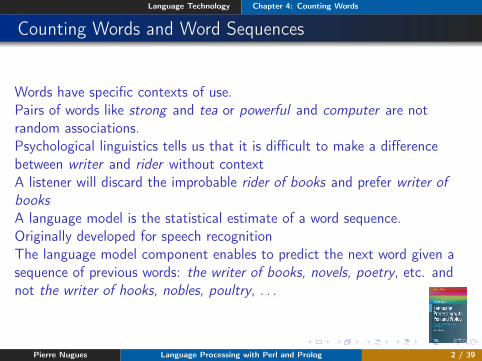
Counting Words and Word Sequences
Words have specific contexts of use.Pairs of words like strong and tea or powerful and computer are notrandom associations.Psychological linguistics tells us that it is difficult to make a differencebetween writer and rider without contextA listener will discard the improbable rider of books and prefer writer ofbooksA language model is the statistical estimate of a word sequence.Originally developed for speech recognitionThe language model component enables to predict the next word given asequence of previous words: the writer of books, novels, poetry, etc. andnot the writer of hooks, nobles, poultry, . . .
Pierre Nugues Language Processing with Perl and Prolog 2 / 39
Language Technology Chapter 4: Counting Words
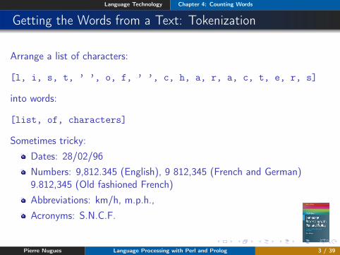
Getting the Words from a Text: Tokenization
Arrange a list of characters:
[l, i, s, t, ’ ’, o, f, ’ ’, c, h, a, r, a, c, t, e, r, s]
into words:
[list, of, characters]
Sometimes tricky:Dates: 28/02/96Numbers: 9,812.345 (English), 9 812,345 (French and German)9.812,345 (Old fashioned French)Abbreviations: km/h, m.p.h.,Acronyms: S.N.C.F.
Pierre Nugues Language Processing with Perl and Prolog 3 / 39
Language Technology Chapter 4: Counting Words
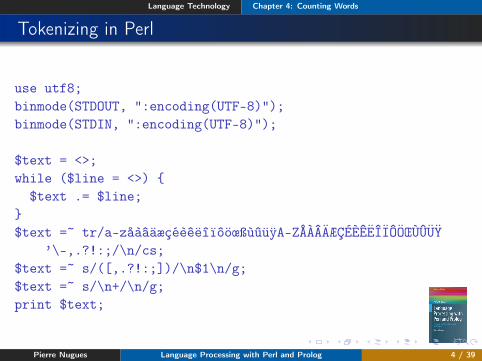
Tokenizing in Perl
use utf8;binmode(STDOUT, ":encoding(UTF-8)");binmode(STDIN, ":encoding(UTF-8)");
$text = <>;while ($line = <>) {
$text .= $line;}$text =~ tr/a-zåàâäæçéèêëîïôöœßùûüÿA-ZÅÀÂÄÆÇÉÈÊËÎÏÔÖŒÙÛÜŸ
’\-,.?!:;/\n/cs;$text =~ s/([,.?!:;])/\n$1\n/g;$text =~ s/\n+/\n/g;print $text;
Pierre Nugues Language Processing with Perl and Prolog 4 / 39
Language Technology Chapter 4: Counting Words
Improving Tokenization
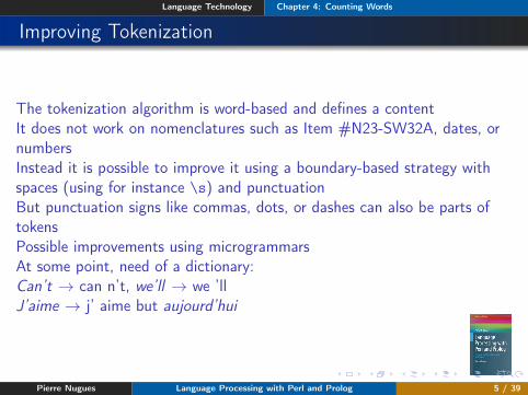
The tokenization algorithm is word-based and defines a contentIt does not work on nomenclatures such as Item #N23-SW32A, dates, ornumbersInstead it is possible to improve it using a boundary-based strategy withspaces (using for instance \s) and punctuationBut punctuation signs like commas, dots, or dashes can also be parts oftokensPossible improvements using microgrammarsAt some point, need of a dictionary:Can’t → can n’t, we’ll → we ’llJ’aime → j’ aime but aujourd’hui
Pierre Nugues Language Processing with Perl and Prolog 5 / 39
Language Technology Chapter 4: Counting Words
Sentence Segmentation
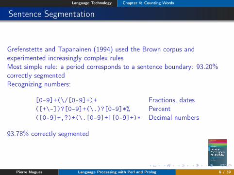
Grefenstette and Tapanainen (1994) used the Brown corpus andexperimented increasingly complex rulesMost simple rule: a period corresponds to a sentence boundary: 93.20%correctly segmentedRecognizing numbers:
[0-9]+(\/[0-9]+)+ Fractions, dates([+\-])?[0-9]+(\.)?[0-9]*% Percent([0-9]+,?)+(\.[0-9]+|[0-9]+)* Decimal numbers
93.78% correctly segmented
Pierre Nugues Language Processing with Perl and Prolog 6 / 39
Language Technology Chapter 4: Counting Words
Abbreviations
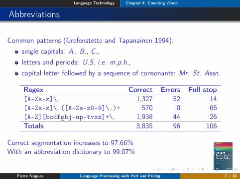
Common patterns (Grefenstette and Tapanainen 1994):single capitals: A., B., C.,letters and periods: U.S. i.e. m.p.h.,capital letter followed by a sequence of consonants: Mr. St. Assn.
Regex Correct Errors Full stop[A-Za-z]\. 1,327 52 14[A-Za-z]\.([A-Za-z0-9]\.)+ 570 0 66[A-Z][bcdfghj-np-tvxz]+\. 1,938 44 26Totals 3,835 96 106
Correct segmentation increases to 97.66%With an abbreviation dictionary to 99.07%
Pierre Nugues Language Processing with Perl and Prolog 7 / 39
Language Technology Chapter 4: Counting Words
N-Grams
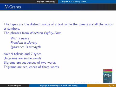
The types are the distinct words of a text while the tokens are all the wordsor symbols.The phrases from Nineteen Eighty-Four
War is peaceFreedom is slaveryIgnorance is strength
have 9 tokens and 7 types.Unigrams are single wordsBigrams are sequences of two wordsTrigrams are sequences of three words
Pierre Nugues Language Processing with Perl and Prolog 8 / 39
Language Technology Chapter 4: Counting Words
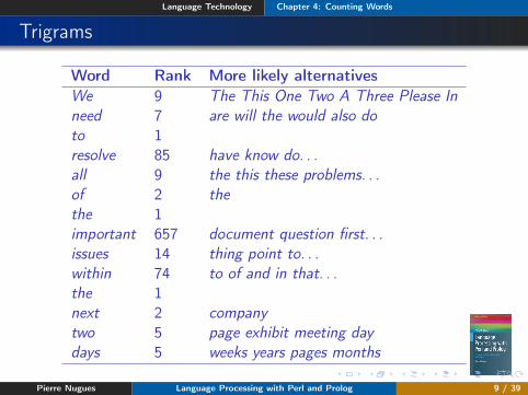
Trigrams
Word Rank More likely alternativesWe 9 The This One Two A Three Please Inneed 7 are will the would also doto 1resolve 85 have know do. . .all 9 the this these problems. . .of 2 thethe 1important 657 document question first. . .issues 14 thing point to. . .within 74 to of and in that. . .the 1next 2 companytwo 5 page exhibit meeting daydays 5 weeks years pages months
Pierre Nugues Language Processing with Perl and Prolog 9 / 39
Language Technology Chapter 4: Counting Words
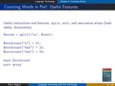
Counting Words in Perl: Useful Features
Useful instructions and features: split, sort, and associative arrays (hashtables, dictionaries):
@words = split(/\n/, $text);
$wordcount{"a"} = 21;$wordcount{"And"} = 10;$wordcount{"the"} = 18;
keys %wordcountsort array
Pierre Nugues Language Processing with Perl and Prolog 10 / 39
Language Technology Chapter 4: Counting Words
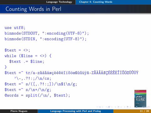
Counting Words in Perl
use utf8;binmode(STDOUT, ":encoding(UTF-8)");binmode(STDIN, ":encoding(UTF-8)");
$text = <>;while ($line = <>) {
$text .= $line;}$text =~ tr/a-zåàâäæçéèêëîïôöœßùûüÿA-ZÅÀÂÄÆÇÉÈÊËÎÏÔÖŒÙÛÜŸ
’\-,.?!:;/\n/cs;$text =~ s/([,.?!:;])/\n$1\n/g;$text =~ s/\n+/\n/g;@words = split(/\n/, $text);
Pierre Nugues Language Processing with Perl and Prolog 11 / 39
Language Technology Chapter 4: Counting Words
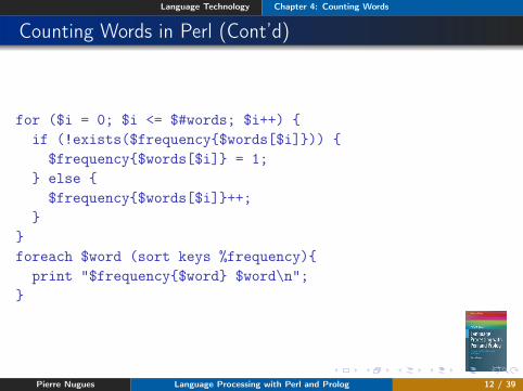
Counting Words in Perl (Cont’d)
for ($i = 0; $i <= $#words; $i++) {if (!exists($frequency{$words[$i]})) {
$frequency{$words[$i]} = 1;} else {
$frequency{$words[$i]}++;}
}foreach $word (sort keys %frequency){
print "$frequency{$word} $word\n";}
Pierre Nugues Language Processing with Perl and Prolog 12 / 39
Language Technology Chapter 4: Counting Words
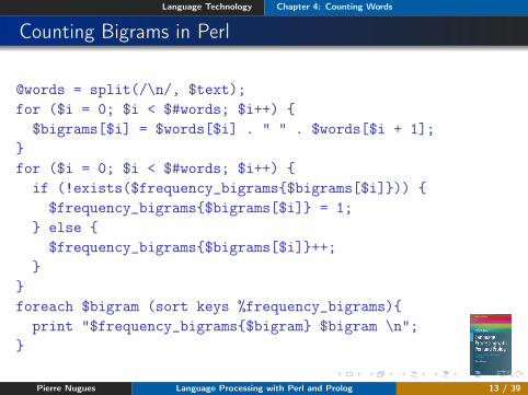
Counting Bigrams in Perl
@words = split(/\n/, $text);for ($i = 0; $i < $#words; $i++) {
$bigrams[$i] = $words[$i] . " " . $words[$i + 1];}for ($i = 0; $i < $#words; $i++) {
if (!exists($frequency_bigrams{$bigrams[$i]})) {$frequency_bigrams{$bigrams[$i]} = 1;
} else {$frequency_bigrams{$bigrams[$i]}++;
}}foreach $bigram (sort keys %frequency_bigrams){
print "$frequency_bigrams{$bigram} $bigram \n";}
Pierre Nugues Language Processing with Perl and Prolog 13 / 39
Language Technology Chapter 4: Counting Words
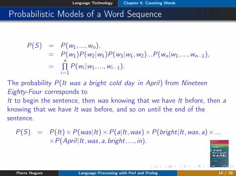
Probabilistic Models of a Word Sequence
P(S) = P(w1, ...,wn),= P(w1)P(w2|w1)P(w3|w1,w2)...P(wn|w1, ...,wn−1),
=n
∏i=1
P(wi |w1, ...,wi−1).
The probability P(It was a bright cold day in April) from NineteenEighty-Four corresponds toIt to begin the sentence, then was knowing that we have It before, then aknowing that we have It was before, and so on until the end of thesentence.
P(S) = P(It)×P(was|It)×P(a|It,was)×P(bright|It,was,a)× ...×P(April |It,was,a,bright, ..., in).
Pierre Nugues Language Processing with Perl and Prolog 14 / 39
Language Technology Chapter 4: Counting Words
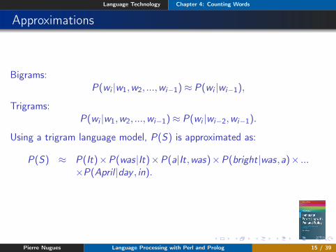
Approximations
Bigrams:P(wi |w1,w2, ...,wi−1)≈ P(wi |wi−1),
Trigrams:P(wi |w1,w2, ...,wi−1)≈ P(wi |wi−2,wi−1).
Using a trigram language model, P(S) is approximated as:
P(S) ≈ P(It)×P(was|It)×P(a|It,was)×P(bright|was,a)× ...×P(April |day , in).
Pierre Nugues Language Processing with Perl and Prolog 15 / 39
Language Technology Chapter 4: Counting Words
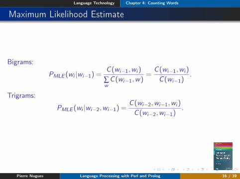
Maximum Likelihood Estimate
Bigrams:
PMLE (wi |wi−1) =C (wi−1,wi )
∑wC (wi−1,w)
=C (wi−1,wi )
C (wi−1).
Trigrams:
PMLE (wi |wi−2,wi−1) =C (wi−2,wi−1,wi )
C (wi−2,wi−1).
Pierre Nugues Language Processing with Perl and Prolog 16 / 39
Language Technology Chapter 4: Counting Words
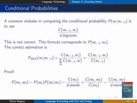
Conditional Probabilities
A common mistake in computing the conditional probability P(wi |wi−1) isto use
C (wi−1,wi )
#bigrams.
This is not correct. This formula corresponds to P(wi−1,wi ).The correct estimation is
PMLE (wi |wi−1) =C (wi−1,wi )
∑wC (wi−1,w)
=C (wi−1,wi )
C (wi−1).
Proof:
P(w1,w2) = P(w1)P(w2|w1) =C (w1)
#words× C (w1,w2)
C (w1)=
C (w1,w2)
#words
Pierre Nugues Language Processing with Perl and Prolog 17 / 39
Language Technology Chapter 4: Counting Words
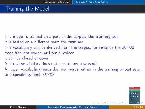
Training the Model
The model is trained on a part of the corpus: the training setIt is tested on a different part: the test setThe vocabulary can be derived from the corpus, for instance the 20,000most frequent words, or from a lexiconIt can be closed or openA closed vocabulary does not accept any new wordAn open vocabulary maps the new words, either in the training or test sets,to a specific symbol, <UNK>
Pierre Nugues Language Processing with Perl and Prolog 18 / 39
Language Technology Chapter 4: Counting Words
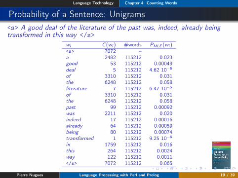
Probability of a Sentence: Unigrams<s> A good deal of the literature of the past was, indeed, already beingtransformed in this way </s>
wi C(wi ) #words PMLE (wi )<s> 7072 –a 2482 115212 0.023good 53 115212 0.00049deal 5 115212 4.62 10−5
of 3310 115212 0.031the 6248 115212 0.058literature 7 115212 6.47 10−5
of 3310 115212 0.031the 6248 115212 0.058past 99 115212 0.00092was 2211 115212 0.020indeed 17 115212 0.00016already 64 115212 0.00059being 80 115212 0.00074transformed 1 115212 9.25 10−6
in 1759 115212 0.016this 264 115212 0.0024way 122 115212 0.0011</s> 7072 115212 0.065
Pierre Nugues Language Processing with Perl and Prolog 19 / 39
Language Technology Chapter 4: Counting Words
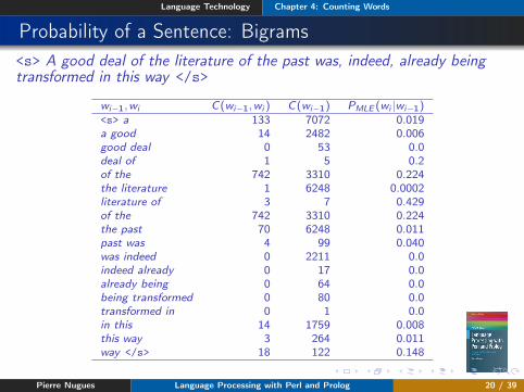
Probability of a Sentence: Bigrams<s> A good deal of the literature of the past was, indeed, already beingtransformed in this way </s>
wi−1,wi C(wi−1,wi ) C(wi−1) PMLE (wi |wi−1)<s> a 133 7072 0.019a good 14 2482 0.006good deal 0 53 0.0deal of 1 5 0.2of the 742 3310 0.224the literature 1 6248 0.0002literature of 3 7 0.429of the 742 3310 0.224the past 70 6248 0.011past was 4 99 0.040was indeed 0 2211 0.0indeed already 0 17 0.0already being 0 64 0.0being transformed 0 80 0.0transformed in 0 1 0.0in this 14 1759 0.008this way 3 264 0.011way </s> 18 122 0.148
Pierre Nugues Language Processing with Perl and Prolog 20 / 39
Language Technology Chapter 4: Counting Words
Sparse Data
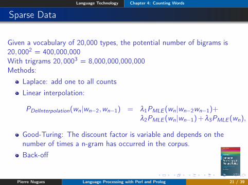
Given a vocabulary of 20,000 types, the potential number of bigrams is20,0002 = 400,000,000With trigrams 20,0003 = 8,000,000,000,000Methods:
Laplace: add one to all countsLinear interpolation:
PDelInterpolation(wn|wn−2,wn−1) = λ1PMLE (wn|wn−2wn−1)+λ2PMLE (wn|wn−1)+λ3PMLE (wn),
Good-Turing: The discount factor is variable and depends on thenumber of times a n-gram has occurred in the corpus.Back-off
Pierre Nugues Language Processing with Perl and Prolog 21 / 39
Language Technology Chapter 4: Counting Words
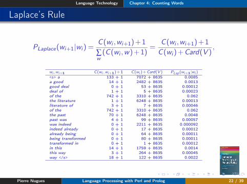
Laplace’s Rule
PLaplace(wi+1|wi ) =C (wi ,wi+1)+1∑w(C (wi ,w)+1)
=C (wi ,wi+1)+1C (wi )+Card(V )
,
wi ,wi+1 C(wi ,wi+1)+1 C(wi )+Card(V ) PLap(wi+1|wi )
<s> a 133 + 1 7072 + 8635 0.0085a good 14 + 1 2482 + 8635 0.0013good deal 0 + 1 53 + 8635 0.00012deal of 1 + 1 5 + 8635 0.00023of the 742 + 1 3310 + 8635 0.062the literature 1 + 1 6248 + 8635 0.00013literature of 3 + 1 7 + 8635 0.00046of the 742 + 1 3310 + 8635 0.062the past 70 + 1 6248 + 8635 0.0048past was 4 + 1 99 + 8635 0.00057was indeed 0 + 1 2211 + 8635 0.000092indeed already 0 + 1 17 + 8635 0.00012already being 0 + 1 64 + 8635 0.00011being transformed 0 + 1 80 + 8635 0.00011transformed in 0 + 1 1 + 8635 0.00012in this 14 + 1 1759 + 8635 0.0014this way 3 + 1 264 + 8635 0.00045way </s> 18 + 1 122 + 8635 0.0022
Pierre Nugues Language Processing with Perl and Prolog 22 / 39
Language Technology Chapter 4: Counting Words
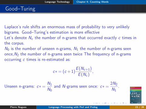
Good–Turing
Laplace’s rule shifts an enormous mass of probability to very unlikelybigrams. Good–Turing’s estimation is more effectiveLet’s denote Nc the number of n-grams that occurred exactly c times inthe corpus.N0 is the number of unseen n-grams, N1 the number of n-grams seenonce,N2 the number of n-grams seen twice The frequency of n-gramsoccurring c times is re-estimated as:
c∗= (c+1)E (Nc+1)
E (Nc),
Unseen n-grams: c∗= N1
N0and N-grams seen once: c∗= 2N2
N1.
Pierre Nugues Language Processing with Perl and Prolog 23 / 39
Language Technology Chapter 4: Counting Words
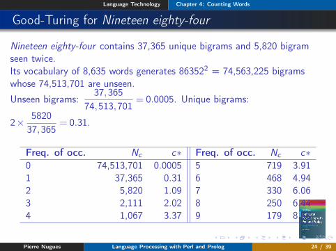
Good-Turing for Nineteen eighty-four
Nineteen eighty-four contains 37,365 unique bigrams and 5,820 bigramseen twice.Its vocabulary of 8,635 words generates 863522 = 74,563,225 bigramswhose 74,513,701 are unseen.
Unseen bigrams:37,365
74,513,701= 0.0005. Unique bigrams:
2× 582037,365
= 0.31.
Freq. of occ. Nc c∗ Freq. of occ. Nc c∗0 74,513,701 0.0005 5 719 3.911 37,365 0.31 6 468 4.942 5,820 1.09 7 330 6.063 2,111 2.02 8 250 6.444 1,067 3.37 9 179 8.93
Pierre Nugues Language Processing with Perl and Prolog 24 / 39
Language Technology Chapter 4: Counting Words
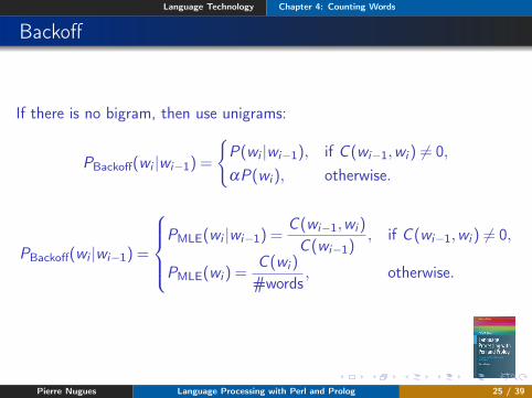
Backoff
If there is no bigram, then use unigrams:
PBackoff(wi |wi−1) =
{P(wi |wi−1), if C (wi−1,wi ) 6= 0,αP(wi ), otherwise.
PBackoff(wi |wi−1) =
PMLE(wi |wi−1) =
C (wi−1,wi )
C (wi−1), if C (wi−1,wi ) 6= 0,
PMLE(wi ) =C (wi )
#words, otherwise.
Pierre Nugues Language Processing with Perl and Prolog 25 / 39
Language Technology Chapter 4: Counting Words
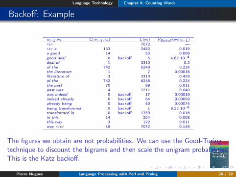
Backoff: Example
wi−1,wi C(wi−1,wi ) C(wi ) PBackoff (wi |wi−1)<s> 7072 —<s> a 133 2482 0.019a good 14 53 0.006good deal 0 backoff 5 4.62 10−5deal of 1 3310 0.2of the 742 6248 0.224the literature 1 7 0.00016literature of 3 3310 0.429of the 742 6248 0.224the past 70 99 0.011past was 4 2211 0.040was indeed 0 backoff 17 0.00016indeed already 0 backoff 64 0.00059already being 0 backoff 80 0.00074being transformed 0 backoff 1 9.25 10−6transformed in 0 backoff 1759 0.016in this 14 264 0.008this way 3 122 0.011way </s> 18 7072 0.148
The figures we obtain are not probabilities. We can use the Good-Turingtechnique to discount the bigrams and then scale the unigram probabilities.This is the Katz backoff.
Pierre Nugues Language Processing with Perl and Prolog 26 / 39
Language Technology Chapter 4: Counting Words
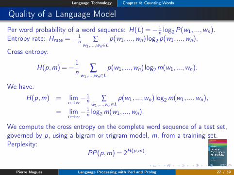
Quality of a Language Model
Per word probability of a word sequence: H(L) =− 1n log2P(w1, ...,wn).
Entropy rate: Hrate =− 1n ∑
w1,...,wn∈Lp(w1, ...,wn) log2 p(w1, ...,wn),
Cross entropy:
H(p,m) =−1n ∑
w1,...,wn∈L
p(w1, ...,wn) log2m(w1, ...,wn).
We have:
H(p,m) = limn→∞− 1
n ∑w1,...,wn∈L
p(w1, ...,wn) log2m(w1, ...,wn),
= limn→∞− 1
n log2m(w1, ...,wn).
We compute the cross entropy on the complete word sequence of a test set,governed by p, using a bigram or trigram model, m, from a training set.Perplexity:
PP(p,m) = 2H(p,m).
Pierre Nugues Language Processing with Perl and Prolog 27 / 39
Language Technology Chapter 4: Counting Words
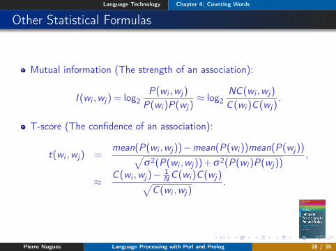
Other Statistical Formulas
Mutual information (The strength of an association):
I (wi ,wj) = log2P(wi ,wj)
P(wi )P(wj)≈ log2
NC (wi ,wj)
C (wi )C (wj).
T-score (The confidence of an association):
t(wi ,wj) =mean(P(wi ,wj))−mean(P(wi ))mean(P(wj))√
σ2(P(wi ,wj))+σ2(P(wi )P(wj)),
≈C (wi ,wj)− 1
NC (wi )C (wj)√C (wi ,wj)
.
Pierre Nugues Language Processing with Perl and Prolog 28 / 39
Language Technology Chapter 4: Counting Words
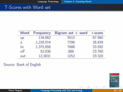
T-Scores with Word set
Word Frequency Bigram set + word t-scoreup 134,882 5512 67.980a 1,228,514 7296 35.839to 1,375,856 7688 33.592off 52,036 888 23.780out 12,3831 1252 23.320
Source: Bank of English
Pierre Nugues Language Processing with Perl and Prolog 29 / 39
Language Technology Chapter 4: Counting Words
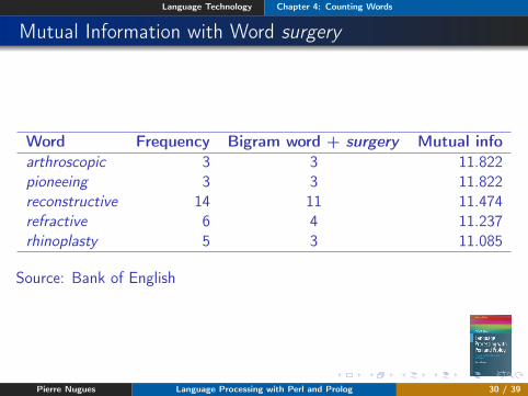
Mutual Information with Word surgery
Word Frequency Bigram word + surgery Mutual infoarthroscopic 3 3 11.822pioneeing 3 3 11.822reconstructive 14 11 11.474refractive 6 4 11.237rhinoplasty 5 3 11.085
Source: Bank of English
Pierre Nugues Language Processing with Perl and Prolog 30 / 39
Language Technology Chapter 4: Counting Words
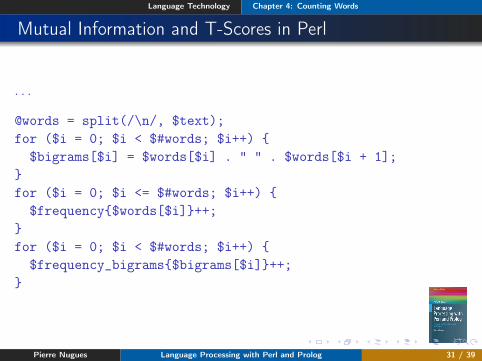
Mutual Information and T-Scores in Perl
. . .
@words = split(/\n/, $text);for ($i = 0; $i < $#words; $i++) {
$bigrams[$i] = $words[$i] . " " . $words[$i + 1];}for ($i = 0; $i <= $#words; $i++) {
$frequency{$words[$i]}++;}for ($i = 0; $i < $#words; $i++) {
$frequency_bigrams{$bigrams[$i]}++;}
Pierre Nugues Language Processing with Perl and Prolog 31 / 39
Language Technology Chapter 4: Counting Words
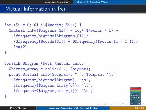
Mutual Information in Perl
for ($i = 0; $i < $#words; $i++) {$mutual_info{$bigrams[$i]} = log(($#words + 1) *
$frequency_bigrams{$bigrams[$i]}/($frequency{$words[$i]} * $frequency{$words[$i + 1]}))/log(2);
}
foreach $bigram (keys %mutual_info){@bigram_array = split(/ /, $bigram);print $mutual_info{$bigram}, " ", $bigram, "\t",
$frequency_bigrams{$bigram}, "\t",$frequency{$bigram_array[0]}, "\t",$frequency{$bigram_array[1]}, "\n";
}
Pierre Nugues Language Processing with Perl and Prolog 32 / 39
Language Technology Chapter 4: Counting Words
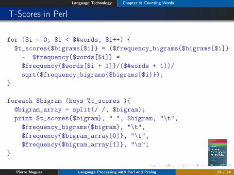
T-Scores in Perl
for ($i = 0; $i < $#words; $i++) {$t_scores{$bigrams[$i]} = ($frequency_bigrams{$bigrams[$i]}
- $frequency{$words[$i]} *$frequency{$words[$i + 1]}/($#words + 1))/sqrt($frequency_bigrams{$bigrams[$i]});
}
foreach $bigram (keys %t_scores ){@bigram_array = split(/ /, $bigram);print $t_scores{$bigram}, " ", $bigram, "\t",
$frequency_bigrams{$bigram}, "\t",$frequency{$bigram_array[0]}, "\t",$frequency{$bigram_array[1]}, "\n";
}
Pierre Nugues Language Processing with Perl and Prolog 33 / 39
Language Technology Chapter 4: Counting Words
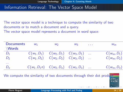
Information Retrieval: The Vector Space Model
The vector space model is a technique to compute the similarity of twodocuments or to match a document and a query.The vector space model represents a document in word space:
Documents\Words
w1 w2 w3 . . . wm
D1 C (w1,D1) C (w2,D1) C (w3,D1) ... C (wm,D1)D2 C (w1,D2) C (w2,D2) C (w3,D2) ... C (wm,D2)...Dn C (w1,D1n) C (w2,Dn) C (w3,Dn) ... C (wm,Dn)
We compute the similarity of two documents through their dot product.
Pierre Nugues Language Processing with Perl and Prolog 34 / 39
Language Technology Chapter 4: Counting Words
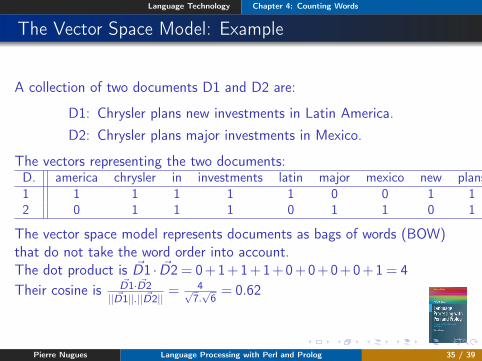
The Vector Space Model: Example
A collection of two documents D1 and D2 are:
D1: Chrysler plans new investments in Latin America.D2: Chrysler plans major investments in Mexico.
The vectors representing the two documents:D. america chrysler in investments latin major mexico new plans1 1 1 1 1 1 0 0 1 12 0 1 1 1 0 1 1 0 1
The vector space model represents documents as bags of words (BOW)that do not take the word order into account.The dot product is ~D1 · ~D2= 0+1+1+1+0+0+0+0+1= 4Their cosine is ~D1· ~D2
|| ~D1||.|| ~D2||= 4√
7.√6= 0.62
Pierre Nugues Language Processing with Perl and Prolog 35 / 39
Language Technology Chapter 4: Counting Words
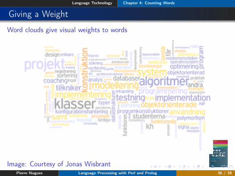
Giving a Weight
Word clouds give visual weights to words
!
Image: Courtesy of Jonas WisbrantPierre Nugues Language Processing with Perl and Prolog 36 / 39
Language Technology Chapter 4: Counting Words
TF × IDF
The frequency alone might be misleadingDocument coordinates are in fact tf × idf : Term frequency by inverteddocument frequency.Term frequency tfi ,j : frequency of term j in document i
Inverted document frequency: idfj = log(N
nj)
Pierre Nugues Language Processing with Perl and Prolog 37 / 39
Language Technology Chapter 4: Counting Words
Document Similarity
Documents are vectors where coordinates could be the count of each word:~d = (C (w1),C (w2),C (w3), ...,C (wn))The similarity between two documents or a query and a document is givenby their cosine:
cos(~q,~d) =
n
∑i=1
qidi√n
∑i=1
q2i
√n
∑i=1
d2i
.
Application: Lucene, Wikipedia
Pierre Nugues Language Processing with Perl and Prolog 38 / 39
Language Technology Chapter 4: Counting Words
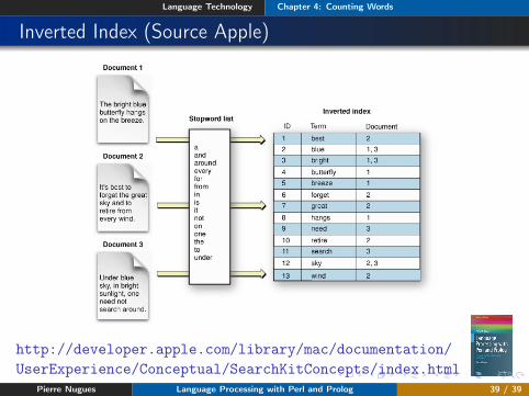
Inverted Index (Source Apple)
http://developer.apple.com/library/mac/documentation/UserExperience/Conceptual/SearchKitConcepts/index.html
Pierre Nugues Language Processing with Perl and Prolog 39 / 39