HAL Id: hal-01985256https://hal.archives-ouvertes.fr/hal-01985256

Submitted on 17 Jan 2019

HAL is a multi-disciplinary open accessarchive for the deposit and dissemination of sci-entific research documents, whether they are pub-lished or not. The documents may come fromteaching and research institutions in France orabroad, or from public or private research centers.

L’archive ouverte pluridisciplinaire HAL, estdestinée au dépôt et à la diffusion de documentsscientifiques de niveau recherche, publiés ou non,émanant des établissements d’enseignement et derecherche français ou étrangers, des laboratoirespublics ou privés.

Lapse tables for lapse risk management in insurance: acompeting risk approach

Xavier Milhaud, Christophe Dutang

To cite this version:Xavier Milhaud, Christophe Dutang. Lapse tables for lapse risk management in insurance: a com-peting risk approach. European Actuarial Journal, Springer, 2018, 8 (1), pp.97-126. �10.1007/s13385-018-0165-7�. �hal-01985256�

Lapse tables for lapse risk management in insurance:

a competing risk approach

Xavier Milhaud∗, Christophe Dutang†

October 21, 2017

Abstract

This paper deals with the crucial problem of modelling policyholders’ behaviours in life insurance.We focus here on the surrender behaviours and model the contract lifetime through the use ofsurvival regression models. Standard models fail at giving acceptable forecasts for the timingof surrenders because of too much heterogeneity, whereas the competing risk framework providesinteresting insights and more accurate predictions. Numerical results follow from using F&G model(Fine & Gray (1999)) on an insurance portfolio embedding Whole Life contracts: through backtests,this framework reveals to be quite efficient and recovers the empirical lapse rate trajectory byaggregating individual predicted lifetimes. These results could be particularly useful to designfuture insurance product. Moreover, this setting allows to calibrate experimental lapse tables,simplifying the lapse risk management for operational teams.

Keywords: life insurance, lifetime, surrender, lapse, competing risks, cumulative incidence functions.

1 Introduction

Lapses correspond to “the expiration of all rights and obligations under an insurance contract if thepolicyholder fails to comply with certain obligations required to uphold those” 1. In terms of financialconsequences, lapse risk is one of the biggest risks to consider for life insurers. Lapses strongly affectinsurers’ Asset and Liabilities Management (ALM) since they trigger unexpected cash flows, andmodify the insurers’ commitments through changes in contractual guarantees.

In this paper, we aim to provide an accurate prediction for the timing of policyholder’s lapse.More precisely, we focus on surrenders, where surrenders are part of the underwriting risk module inthe Solvency II directive and are defined 1 as “the (premature) termination of an insurance contractby the policyholder”. In this case, the insurer has to pay the policyholder or its beneficiary thesurrender value (or cash value) which is contractually agreed. Lapses thus include surrenders, butalso other causes of termination: death, default on premium payments, maturity, or else. That being

∗Universite de Lyon, Universite Lyon 1, ISFA, Laboratoire SAF, 50 Avenue Tony Garnier, F-69007 Lyon.†Laboratoire Manceau de Mathematiques, Universite du Maine, Avenue Olivier Messaien, F-72000 Le Mans.1See http://ec.europa.eu/finance/insurance/docs/solvency/impactassess/annex-c08d en.pdf

1

said, it seems natural to consider a competing risk approach since these causes of lapse are mutuallyexclusive (Laurent et al. (2016)). For sure, someone who dies cannot surrender her contract, or adefault on premium payments has nothing to do with contractual maturity. Surprisingly, there is nosuch approach in the literature concerning the lapse modelling within a regression framework, thoughit is a standard tool to model prepayments in the banking sector. Many empirical studies show thatthe surrender rate drives the lapse rate trajectory in life insurance companies: indeed this trajectorybasically results from policyholders’ decisions, but do not significantly depend on other unvoluntaryevents (e.g. death) that remain quite stable in proportion over time. That is the reason why this paperfocuses on surrender behaviours.

In practice, it is crucial for insurers to model not only the surrender decision but also its timing,because initial expenses to issue the contract as well as associated management costs cannot berecovered in case of early surrenders. This means that the insurer must pay a particular attention tothe product design to avoid this, but more on that in Section 2 through our real-life analysis. Basedon this idea, we adopt a survival analysis framework combined to a competing risk approach. To thebest of our knowledge, lapse risk has never been modeled this way: the novelty of our work lies inthe consideration of the subdistribution approach to model the contract survival probability relatedto surrenders. There exist many other statistical approaches available in the literature to modelsurrenders: generalized linear models (GLM) were often used in the past (Cox & Lin (2006), Milhaud(2013)), as well as financial mathematics techniques (to price the surrender option, see Bacinello(2005), Bacinello et al. (2008)) or temporal series and cointegration (Kuo et al. (2003)). However,they all suffer from “unacceptable” drawbacks: a selection bias is introduced when using GLM onmultiple periods, the assumption of agent’s rationality is very strong in the second case, and theheterogeneity of policyholders’ behaviours cannot be captured within the last approach. To assess thefinancial consequences of lapses on the insurer balance sheet, please refer to the interesting papers byBuchardt (2014) and Buchardt et al. (2015) (competing risks appear therein, but there is no focus onindividual risk factors that impact the surrender rate).

In this competing risk framework, the surrender is our cause of interest. In this perspective, wedevelop a survival regression model which allows to predict the individual contract lifetime before sur-render given a set of risk factors affecting the propensity to terminate the contract. Most of time,practitioners suggest to distinguish structural from temporary surrenders: the firsts relate to surren-ders due to personal projects (e.g. purchase a car, buy a new house, which is not independent from thepolicyholder’s age for instance), whereas others are triggered by adverse scenarios concerning the con-ditions surrounding the insurance contract (e.g. bad macroeconomic conditions, firm reputation). Inthis view, the model has to integrate various effects, from idiosyncratic risk factors (Outreville (1990))to external information (e.g. a financial market index linked to the insurance contract profitability, seeKim (2005) or Russell et al. (2013)). Roughly speaking, the model should be flexible enough to takeinto account the heterogeneity of policyholders’ behaviours facing different situations. In this context,we show hereafter that the F&G model (Fine & Gray (1999)) provides satisfying results and enablesto get accurate predictions of contract lifetime depending on policyholder’s characteristics, contractfeatures and financial environment.

The paper is organized as follows: Section 2 presents the portfolio and the insurance product underconsideration. Some general descriptive statistics are provided. In Section 3, we explain the differencesbetween the cause-specific and the subdistribution approaches in a competing risk framework: despitebeing the most famous one, the former approach tends to be unadapted to our context. To illustratethis, we give a practical example which shows that the estimation of the surrender intensity can bestrongly biased because of the misestimation of intensities related to other (rare) events. Then we

2

build an optimal model in Section 4, which is validated in Section 5 through classical test statisticsapplied to the learning data. Furthermore, we check for its prediction power by two methodologies:i) we compare predicted and observed surrender rates (computed from the agregation of individuallifetimes), and ii) we compare predicted and observed survival probabilities by risk profile. Finallyand in the same spirit as CSO tables for mortality in US, we propose to build multidimensionalexperimental surrender tables in Section 6.

2 Context and portfolio under study

In this section, we first describe the general context corresponding to our study and give some particularfeatures of the product under consideration. Our simulated dataset is largely inspired by a real-lifeportfolio provided by a private insurer operating in US.

Life insurance in US can roughly be divided into two families: either Term Life or Whole Lifecontracts. Term Life contracts concerns temporary insurance contracts which guarantees a capitalagainst the death of the insured (e.g. a mortgage life insurance) and does not accumulate a cash value.On the contrary, Whole Life insurance deals with permanent insurance contracts which accumulates acash value and terminates at the death of the policyholder. Our data deals with Whole Life policies,where the policyholder may voluntary cancel her contract (possibly with penalties in case of earlywithdrawals).

Typically, Whole Life insurance comes along with a minimum death benefit (nominal value), amaturity benefit on the cash value (the minimum between the nominal and the economic value ofthe unit-linked account), and sometimes with riders which guarantee extra cash amount in case ofpredetermined events (e.g. accidental death). The underwriting of such policies assumes the paymentof a contractual premium. That premium can be paid periodically (e.g. every month), or as a lumpsum at the beginning. This particular feature may have an impact on the customer behaviour: eitherattachment to the contract because of the regular contribution, or tiredness. The premium dependson at least four features: the nominal value, the policyholder’s age and gender, and the tobaccoconsumption.

Expenses and commissions are added up to the pure premium. The corresponding rates dependmainly on the distribution channel: brokers and tied-agents are not similarly compensated. In Table1, we present the commission and the expense rates generally used for Whole Life contracts sold bytied-agents. Notably, the commission rate is very high in the first year of the contract and falls tozero after the tenth year. Therefore, the tied-agent may have an incentive to force customers to moveto a new contract with higher commissions for him. It is also important to mention that the expenserates vary depending on the premium frequency. The general rule is: the more frequent the premiumis paid, the higher the expenses.

Type (nominal > 10000$) 1st year 2-10 years 11+ years

Commission 50% 4% 0%

Management expense 0% 2% 3%

Total 50% 6% 3%

Table 1: Commissions and expense as percentage of the annual premium.

3

As already mentioned, the policyholder may choose to surrender her life insurance policy in orderto immediately retrieve the cash value. However, the policyholder faces potential penalties. Forexample in France, there are 35% of tax on capital gains of the contract if the withdrawal happensbefore the fourth year, 15% between the fifth and the seventh year, and only 7.5% above an increasingthreshold afterwards. In US (our setting), surrender charges also apply if a withdrawal occurs duringthe surrender period (from 10 to 15 years). Here, the surrender charge is 100% on the cash value inthe first three years and then linearly decreases as time elapses. This feature is a clear incentive tokeep the contracts in force at least three years, and then as long as possible.

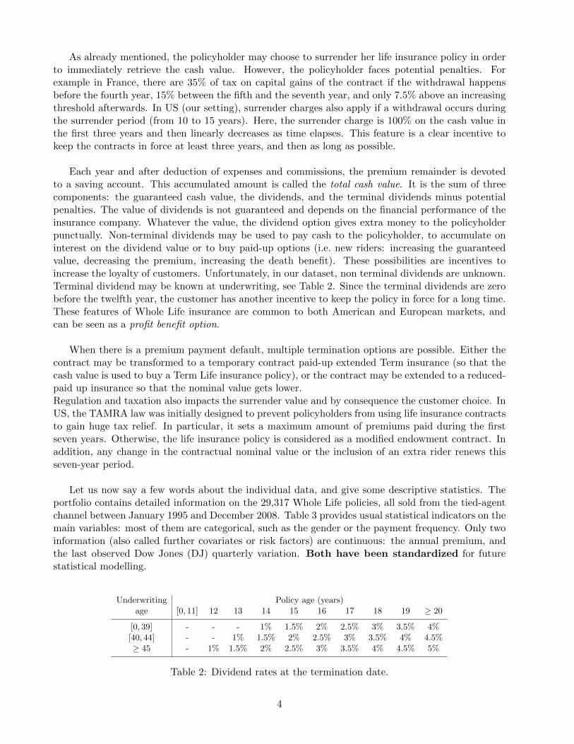
Each year and after deduction of expenses and commissions, the premium remainder is devotedto a saving account. This accumulated amount is called the total cash value. It is the sum of threecomponents: the guaranteed cash value, the dividends, and the terminal dividends minus potentialpenalties. The value of dividends is not guaranteed and depends on the financial performance of theinsurance company. Whatever the value, the dividend option gives extra money to the policyholderpunctually. Non-terminal dividends may be used to pay cash to the policyholder, to accumulate oninterest on the dividend value or to buy paid-up options (i.e. new riders: increasing the guaranteedvalue, decreasing the premium, increasing the death benefit). These possibilities are incentives toincrease the loyalty of customers. Unfortunately, in our dataset, non terminal dividends are unknown.Terminal dividend may be known at underwriting, see Table 2. Since the terminal dividends are zerobefore the twelfth year, the customer has another incentive to keep the policy in force for a long time.These features of Whole Life insurance are common to both American and European markets, andcan be seen as a profit benefit option.

When there is a premium payment default, multiple termination options are possible. Either thecontract may be transformed to a temporary contract paid-up extended Term insurance (so that thecash value is used to buy a Term Life insurance policy), or the contract may be extended to a reduced-paid up insurance so that the nominal value gets lower.Regulation and taxation also impacts the surrender value and by consequence the customer choice. InUS, the TAMRA law was initially designed to prevent policyholders from using life insurance contractsto gain huge tax relief. In particular, it sets a maximum amount of premiums paid during the firstseven years. Otherwise, the life insurance policy is considered as a modified endowment contract. Inaddition, any change in the contractual nominal value or the inclusion of an extra rider renews thisseven-year period.

Let us now say a few words about the individual data, and give some descriptive statistics. Theportfolio contains detailed information on the 29,317 Whole Life policies, all sold from the tied-agentchannel between January 1995 and December 2008. Table 3 provides usual statistical indicators on themain variables: most of them are categorical, such as the gender or the payment frequency. Only twoinformation (also called further covariates or risk factors) are continuous: the annual premium, andthe last observed Dow Jones (DJ) quarterly variation. Both have been standardized for futurestatistical modelling.

Underwriting Policy age (years)age [0, 11] 12 13 14 15 16 17 18 19 ≥ 20

[0, 39] - - - 1% 1.5% 2% 2.5% 3% 3.5% 4%[40, 44] - - 1% 1.5% 2% 2.5% 3% 3.5% 4% 4.5%≥ 45 - 1% 1.5% 2% 2.5% 3% 3.5% 4% 4.5% 5%

Table 2: Dividend rates at the termination date.

4

Variable Statistics Comments

Issue Date between 01/01/1995 for policies not terminated in Dec. 2008,and end of 2008 we have no information: fixed right censored

Time duration min: 0.01; max: 62.09; unknown if policy not terminated(in quarters) mean: 30.26; std: 18.78

Gender male: 50.05%; female: 49.95% no missing value

Payment frequency infra annual: 61.37%; annual: 23.44%; Infra-annual: monthly, quarterly, semi-annual.other (supra annual): 15.19%

Risk state non smoker: 63.01%; smoker: 36.99% no missing value

Underwriting age young: 47.46% between 0 and 34 years oldmiddle: 34.04% between 35 and 54 years oldold: 18.50% between 55 and 84 years old

Living place east coast: 20.62%; west coast: 4.60%: no missing valueother: 74.78%

Annual premium min: -1.07; median: -0.30; max: 12.13 this variable has been standardized.mean: $560.88 ; std: $526.5870 (in original dollar scale)

DowJones Index variation min: -4.53; median: -0.38; max: 2.43 this variable has been standardized.mean: 0.001781 ; std: 0.049413 (in original scale)

Accidental death rider yes: 16.42%; no: 83.58%

Termination cause 0: 49.06% in force1: 38.22% surrender2: 12.72% cancellation (other causes: death, term,. . . )

Death indicator 0: 95.62% alive1: 4.38% dead

Table 3: List of main variables in our database.

To visualize the data, we use traditional boxplots where the width of the boxplot is proportionalto the exposure of each variable category in the whole dataset. In Figure 1, we represent the boxplotof the duration with respect to the termination cause (i.e. no termination, surrender, cancellation).We logically observe that the duration of the policy is much longer for in-force policies than thosethat have been terminated. In average the contract lifetime is close to 14 quarters for surrenderedcontracts, whereas half of the contracts experience at least 45 quarters of duration. These statementsare in line with the aforementioned product features.

Similar boxplots can be obtained from other categorical covariates, but are not illustrated here sincethe differences in terms of duration for each category are not as convincing as for the termination cause.Instead, we present in Table 4 the results of the Kruskal-Wallis test (χ2 statistic) for independencebetween the lifetime and the categorical variable under study. All variables except the living place ofthe policyholder are statistically not independent to the surrender decision. It thus makes sense toanalyze them in the coming modeling section, yet the living place should not appear to be relevant.

Surrender Termination Acc Rider Gender Under. Age Living place Risk state Prem. Freq.

p-value (%) < 10−4 < 10−4 < 10−4 0.0126 0.0001 38.32 0.0157 < 10−4

KW statistic 7626.30 11211.89 27.62 14.70 27.59 1.92 14.29 111.05deg. of freedom 1 2 1 1 2 2 1 2

Table 4: Results of the Kruskal-Wallis rank sum test.

5

Figure 1: Boxplots of duration (in quarters) depending on the termination cause.

In Figure 2, we plot the quarterly lapse and surrender rates all along the observation period (from1995 to 2008). Notice that the two trajectories are similar and have a strong correlation, which showsthat other events than surrenders (e.g. deaths) have a stationnary impact on the lapse rate. Thebarplots in the background represent the number of in-force policies: the biggest exposure in theportfolio happens in 2006.

Figure 2: Exposure and exit rates over time, on the whole sample. The exposure (left y-axis) refersto the number of in-force policies for each quarter, and the right y-axis represents quarterly rates.

In Figure 3, we analyze the effect of two risk factors on the surrender decision: the paymentfrequency and the underwriting age. We have chosen these two variables because they have thehighest statistic value in Table 4. For each category, we also report the surrender rates (in percentage)

6

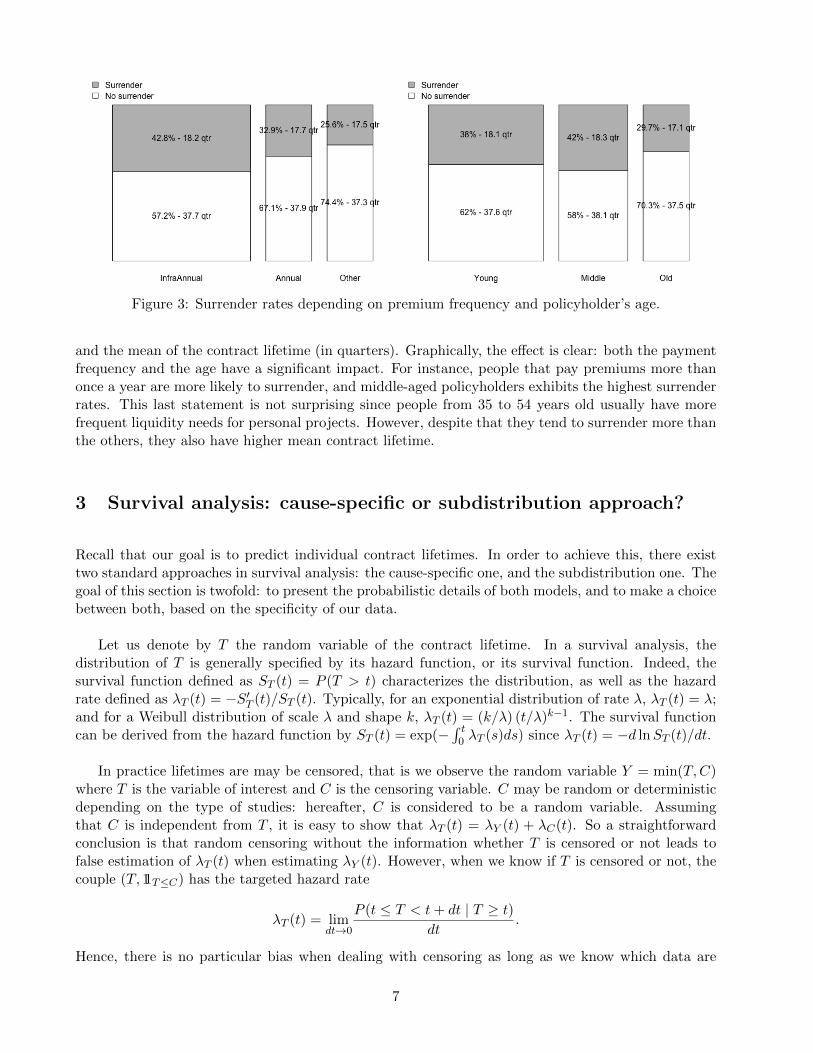
Figure 3: Surrender rates depending on premium frequency and policyholder’s age.

and the mean of the contract lifetime (in quarters). Graphically, the effect is clear: both the paymentfrequency and the age have a significant impact. For instance, people that pay premiums more thanonce a year are more likely to surrender, and middle-aged policyholders exhibits the highest surrenderrates. This last statement is not surprising since people from 35 to 54 years old usually have morefrequent liquidity needs for personal projects. However, despite that they tend to surrender more thanthe others, they also have higher mean contract lifetime.

3 Survival analysis: cause-specific or subdistribution approach?

Recall that our goal is to predict individual contract lifetimes. In order to achieve this, there existtwo standard approaches in survival analysis: the cause-specific one, and the subdistribution one. Thegoal of this section is twofold: to present the probabilistic details of both models, and to make a choicebetween both, based on the specificity of our data.

Let us denote by T the random variable of the contract lifetime. In a survival analysis, thedistribution of T is generally specified by its hazard function, or its survival function. Indeed, thesurvival function defined as ST (t) = P (T > t) characterizes the distribution, as well as the hazardrate defined as λT (t) = −S′T (t)/ST (t). Typically, for an exponential distribution of rate λ, λT (t) = λ;and for a Weibull distribution of scale λ and shape k, λT (t) = (k/λ) (t/λ)k−1. The survival functioncan be derived from the hazard function by ST (t) = exp(−

∫ t0 λT (s)ds) since λT (t) = −d lnST (t)/dt.

In practice lifetimes are may be censored, that is we observe the random variable Y = min(T,C)where T is the variable of interest and C is the censoring variable. C may be random or deterministicdepending on the type of studies: hereafter, C is considered to be a random variable. Assumingthat C is independent from T , it is easy to show that λT (t) = λY (t) + λC(t). So a straightforwardconclusion is that random censoring without the information whether T is censored or not leads tofalse estimation of λT (t) when estimating λY (t). However, when we know if T is censored or not, thecouple (T, 11T≤C) has the targeted hazard rate

λT (t) = limdt→0

P (t ≤ T < t+ dt | T ≥ t)dt

.

Hence, there is no particular bias when dealing with censoring as long as we know which data are

7

censored.

Let us now consider the counting process framework. A counting process (Nt)t is a cadlag stochasticprocess adapted to a filtration with N0 = 0, Nt < +∞ a.s. and jumps of size 1. The well-known Doob-Meyer decomposition, see Fleming & Harrington (2013), states that Nt = Λt + Mt where (Λt)t iscalled the compensator, a non decreasing predictable process and (Mt)t is a local martingale w.r.t.the filtration such that E(Nt) = Λt. In the absolute continuous case, the compensator has the followingform Λt =

∫ t0 λ(s)ds where λ(t) is a predictable process known as the intensity. The very special case

of a constant intensity λ(t) = λ leads to the Poisson process with exponential rate jumps.

A process of particular interest linked to the couple (T, 11T≤C) is Nt = 11T≤t,T≤C , that jumps ifthe time of interest T is below t and non censored. The at-risk process defined as Rt = (11T≥t)tindicates if neither the event nor the censoring occurs before t. (Nt, Rt) is the stochastic processcounterpart of static random variables (T, 11T≤C). Studying n i.i.d. replicates (Ti, 11Ti≤Ci)i=1,...,n leadsto the empirical version of the counting processes by summing over all individuals:

Nt =n∑i=1

11Ti≤t, Ti≤Ci , Rt =

n∑i=1

11min(Ti,Ci)≥t.

One can show that the compensator of Nt is Λt =∫ t0 RsλT (s)ds. The well-known nonparametric

Nelson-Aalen estimator of Λt is defined by Λt =∫ t0 (1/Rs) 11Rs>0 dNs. By the central limit theorem,

the asymptotic distribution of Λt can be obtained.

In a multi-cause framework, see e.g. Martinussen & Scheike (2006), we suppose that at the failuretime we know the cause of the failure. That is we define JT the type of failure among {1, . . . , J}. Theprocess (Jt)t starting with J0 = 0 is a continuous-time random process that jumps at T into a statein {1, . . . , J}. From a multi-state model point-of-view, the multi-cause model is a special case where0 is the initial state and {1, . . . , J} are absorbing states, see Figure 4.

Figure 4: Competing risk model and multistate representation, for j = 1, 2, ..., J .

Let us define cause-specific hazard rates for j ∈ {1, . . . , J} as

λT,j(t) = limdt→0

P (t ≤ T < t+ dt, JT = j | T ≥ t)dt

. (1)

By the formula of total probability, we can retrieve the overall hazard rate by summation of Equation(1): λT,1(t) + · · ·+ λT,J(t) = λT (t), and recover the overall survival distribution of T by

P (T > t) = 1− FT (t) = ST (t) = exp

(−∫ t

0(λT,1(s) + · · ·+ λT,J(s)) ds

).

8

In practice we are interested not in ST but in the following probability FT,j(t) = P (T ≤ t, JT = j),the so-called cumulative incidence function (CIF) for the cause j. Due to the event JT = j, this isnot a proper cumulative distribution function since FT,j(t)→ P (JT = j) as t→ +∞.

For a continuous distribution of T , we characterize it as the integral of a (improper) densityFT,j(t) =

∫ t0 fT,j(s)ds. By conditioning on T ≥ t, the improper density is obtained as the following

limit:

fT,j(s) = limdt→0

P (t ≤ T < t+ dt, JT = j)

dt= λT,j(t)ST (t).

In other words, fT,j(t) is the product of the cause-specific hazard rate and the probability to surviveup to time t. Therefore, the CIF is

FT,j(t) =

∫ t

0λT,j(s) exp

(−∫ s

0λT (u)du

)ds. (2)

Hence, in this framework, the CIF of cause j depends on all other causes via the global survivalfunction, which makes the interpretation of the effects of covariates quite tricky since some effectscome from the overall hazard rate λT (t). The CIF has the good property to be interpretable and

summable P (T ≤ t) = FT,1(s) + · · ·+ FT,J(s), unlike to the function 1− exp(−∫ t0 λT,j(u)du

).

This approach, called the cause-specific approach, thus requires to estimate the hazard rates (1) of allcauses so as to estimate the CIF (2) of cause j.

The concurrent methodology to estimate the CIF of a single cause is possible by considering a newcompeting risk process. Let us assume that cause 1 is our cause of interest. We define τ as

τ = T × 11JT=1 +∞× 11JT 6=1.

The distribution of τ is the same as T for JT = 1, P (τ ≤ t) = FT,1(t) and a mass point at infinity1 − FT,1(∞), probability to observe other causes (JT 6= 1) or not to observe any failure. The hazardrate of τ can be written as

λτ (t) = limdt→0

P (t ≤ T < t+ dt, JT = 1 | {T ≥ t} ∪ {T ≤ t, JT 6= 1})dt

. (3)

Hence the CIF for cause 1 is computed as

FT,1(t) = 1− exp

(−∫ t

0λτ (s)ds

). (4)

Therefore the estimation of the CIF (4) does not depend on the estimation of other causes’ hazardrates. This second approach is called the subdistribution approach, and often leads to different effectsof covariates on the cause-specific hazard function on one side and on the corresponding CIF on theother side (Gray (1988), Pepe (1991)). Without censoring, the process Nτ (t) = 11τ≤t = 11T≤t, JT=1 hasthe compensator

Λτ (t) =

∫ t

0λτ (s)(11T≥s + 11T≤s, JT 6=1) ds.

Taking into account censoring, the nonparametric Nelson-Aalen estimator of Λτ can be adapted to thecompeting risk framework by updating the at-risk process Rt and the counting process Nt accordingly.That is, the numerator is the count of non-censored times Ti ≤ Ci of interest JTi = 1 while thedenominator is the count of non-exited individuals and exited individuals of other causes (JTi 6= 1):

Λτ (t) = 11maxi Ti>t

n∑i=1

11Ti≤t≤Ci,JTi=1

RTi, Rt =

n∑i=1

(1− 11Ti≤t≤Ci,JTi=1),

9

with Yi = min(Ti, Ci).

To illustrate the differences between these two approaches, we consider a randomly selected subsetof our database, and extract the three main causes of termination: surrender, death, and other causesgrouped in a single category (i.e. JT ∈ {1, 2, 3}). Our cause of interest is the surrender cause, denotedby JT = 1. Other causes are tagged as competing risks. On this subset, we fit a simple regressionmodel via the cause-specific approach by considering one single explanatory variable: the risk state.In addition, we fit the same regression model (with the risk state as covariate, related to the smokerstatus) via the subdistribution approach. By construction, the cause-specific approach will providean estimation of three CIFs P (T ≤ t, JT = 1), P (T ≤ t, JT = 2), P (T ≤ t, JT = 3) unlike thesubdistribution approach which only provides P (T ≤ t, JT = 1).

Estimations are plotted in Figure 5. The solid line corresponds to the CIF of non-smoker policy-holders, while the dashed line represents the CIF of smokers. Colored curves stand for the regressionmodel, whereas the black curves correspond to the non-parametric estimation. On the middle and theright-hand graphs, we observe that the CIF estimated by the cause-specific approach are particularlybadly estimated: there is a significant difference with the non-parametric estimation. On the left-handgraph we observe that the estimated CIF are graphically close, irrespectively of the approach. In orderto differentiate these approaches numerically, we compute error statistics2 in Table 5. In overall, theCIF for non-smoker are better estimated than the CIF for smoker (errors three times lower). On thetwo competing risks (causes 2 and 3), the errors are particularly high: from 8 to 90 times higher thanthe error for cause 1. Regarding the cause of interest, the estimation via the subdistribution approachis slightly better than with the cause-specific approach. This is probably due to uncertain estimationsof hazard rates for other causes used when computing the CIF. The difference would probably be muchhigher if there were very few events for one of the different causes of lapse: compensation would beexperienced, which should lead to poor estimation of individual hazard rates. In conclusion to theseresults, we opt for the subdistribution approach in the coming modelling section.

Figure 5: Estimation of the cumulative incidence functions (NS: non-smoker, S: smoker).

4 Model selection

To build the model, the dataset is splitted into two subsamples. Two third of the data, the learningsample, are used to fit the competing risk model. The last third, representing the test sample, will

2See Appendix A for a definition.

10

Sum of absolute relative error Sum of squared relative error

Risk state non-smoker smoker non-smoker smoker

Cause-spec. P (T ≤ t, JT = 1) 11.53 45.66 0.69 76.08Cause-spec P (T ≤ t, JT = 2) 83.40 184.73 44.59 156.91Cause-spec P (T ≤ t, JT = 3) 37.68 135.98 11.46 448.04Subdist. P (T ≤ t, JT = 1) 9.71 39.80 0.62 68.86

Table 5: Goodness of fit statistics: summary of errors related to the CIF estimation.

enable us to assess the performance and the robustness of the selected model in Section 5.

First, let us introduce formally the F&G proportional hazards model, see Fine & Gray (1999).As previously explained, the principle of the subdistribution approach lies in considering a new andartificial at-risk population (this idea already existed in the context of cure models). Integratingcovariates to take into account the individual characteristics of the population (through the vectorX), the subdistribution hazard of this model for surrenders (cause 1 from (4)) is defined by

λτ,1(t; X) := limdt→0

1

dtP (t ≤ T < t+ dt ∩ JT = 1 | {T ≥ t} ∪ {T ≤ t ∩ JT 6= 1},X)

= λ10(t) exp(X(t)′β), (5)

where λ10(t) is a completely unspecified nonnegative function (risk of the reference profile, moredetails further), X(t)′ = (X1(t), ..., Xk(t)) is the vector of the k (time-varying or not) covariates, andβ′ = (β1, ..., βk) is the vector of regression coefficients to be estimated3.

This specification looks like the well known Cox model. However, recall that the at-risk populationis different to take into account the competing risk framework, which has an impact on the estimationof λ10(t) and β. The expression of the hazard λτ,1(t; X) yields to the following formula for the CIF ofsurrenders:

FT,1(t; X) = P (T ≤ t, JT = 1 |X) = 1− exp

(−∫ t

0λ10(s) exp(XT (s)β) ds

). (6)

In order to select an optimal model and make some comparisons at the end, we start by estimating afully nonparametric model (whose regression coefficients are all time-varying). Then, step by step, weintroduce parametric terms through the consideration of constant effect on the response for some co-variates. The selection of introduced parametric terms is made based on statistical tests that measurethe significance of the effects and their type (time-varying versus constant coefficients β). Typically,the supremum test and the Kolmogorov-Smirnov test are used. In the fully nonparametric model,all the regression coefficients are time-varying. On the opposite, the case of only constant regressioncoefficients is the semiparametric model by Fine & Gray (1999), see Equation (5). This procedureallows us to check that considering only constant effects is not too restrictive from a modelling view-point. All the estimations are performed in R (R Core Team (2017)) thanks to the packages timereg(Martinussen & Scheike (2006), Scheike & Zhang (2011)) and cmprsk (Gray (2014)).

To start with, all available covariates of the database were initially inputed in the modelling. Thatis to say accidental death rider, gender, premium frequency, risk state, underwriting age, living place,annual premium, and Dow Jones index (more precisely the relative variation of this index in the lastobserved quarter). The results show that one category of the living place, people living on the West

3’ denotes the transpose.

11

Coast, has a non significant effect on the lifetime before surrender (see Table 12 in Appendix B).We thus aggregate this category with another one (East Coast), and estimate once again the model.Considering living place as a risk factor is still not relevant (see Table 13, still in Appendix B). Theestimation of the model without this variable leads to satisfying results in terms of global significance(Table 14), despite concerns about some effects that should not be considered as time-varying. Indeed,it is clear from Table 15 in Appendix B that some covariates seem to have a constant effect (constantassociated regression coefficients) on the lifetime before surrender.

Looking at the outputs of previous statistical tests, we now estimate an “intermediate” modelin which some of the covariates have a constant effect on the response. These covariates are theunderwriting age and the gender. After having fitted this new model, results show that other covariatesshould also be considered as having constant effects: this is the case of the category annual of thepremium frequency, as well as the category smoker for the risk state. Finally, this process ends up witha model having constant effects (gender, risk state, category annual of premium frequency, categorymiddle of underwriting age) and time-varying effects (category other of premium frequency, categoryold of underwriting age, accidental death rider, annual premium and Dow Jones). Tables 16 and 17in Appendix B provide the numerical outputs of this model. The fact that half of the covariates seemto have a constant effect comforts us in the opportunity to apply the F&G model further, where F&Gmodel is less flexible but more parsimonious (and is thus likely to provide more robust predictions).

Regarding time-varying effects of this intermediate model, we plot in Figure 6 the intercept andthe regression coefficients of the five corresponding variables (namely death rider, premium frequency,underwriting age, annual premium and Dow Jones variation). Notice that the effect of the variationof the Dow Jones Index tends to explode for highest durations. This was also the case with thefully nonparametric approach. The confidence we can have in this estimation is low: the highest theduration, the widest the confidence interval. This is due to the fact that there are very few eventsobserved for such durations. In practice, this means that the propensity to surrender due to thevariation of the Dow Jones Index is likely to be largely overestimated for highest durations.

Let us now focus on the estimation of the F&G proportional hazards model of Equation (5).Beginning with all available covariates, we fit the model by a backward stepwise approach. As in thefully nonparametric modelling, the living place is not significant (associated p-values for each categoryexceed 20%). This is in line with our conclusions following descriptive statistics in Section 2. The nextstep thus consists in performing the estimation without this covariate, still embedding only parametricterms. This procedure comes up with a model that is globally statistically significant, and where everycovariate also has a statistically significant effect. In other words, this is one of the best model in thismodel class. The results of the F&G model are stored in Table 6.

Covariate Coefficient Standard Error Gray’s test statistic p-value

Accidental Death Rider - Yes -0.191 0.0371 -5.16 2.5×10−7

Gender - Female -0.0784 0.0256 -3.06 2.2×10−3

Premium Frequency - Annual -0.222 0.0316 -7.03 2.13×10−12

Premium Frequency - Other -0.395 0.0398 -9.94 0

Risk State - Smoker -0.136 0.0269 -5.04 4.7×10−7

Underwriting Age - Middle 0.121 0.0293 4.12 3.83×10−5

Underwriting Age - Old -0.2 0.0389 -5.14 2.73×10−7

Annual Premium 0.142 0.0116 12.30 0Dow Jones variation 0.889 0.0186 47.90 0

Table 6: Estimated constant regression coefficients in the F&G model.

12

0 10 20 30 40 50

-4-3

-2-1

0

Time

Coefficients

(Intercept)

0 10 20 30 40 50

-0.6

-0.4

-0.2

0.0

0.2

Time

Coefficients

acc.death.riderRider

0 10 20 30 40 50

-1.2

-1.0

-0.8

-0.6

-0.4

-0.2

0.0

Time

Coefficients

premium.frequencyOther

0 10 20 30 40 50

-0.6

-0.4

-0.2

0.0

0.2

Time

Coefficients

underwriting.ageOld

0 10 20 30 40 50

-0.1

0.0

0.1

0.2

Time

Coefficients

annual.premium

0 10 20 30 40 50

12

34

5

Time

Coefficients

DJIA

Figure 6: Estimation of time-varying regression coefficients in the intermediate model.

All the regression coefficients in Table 6 are estimated in comparison to a reference profile, i.e. apolicyholder with the following characteristics in our case: a young non-smoker male with an infra-annual premium frequency, without the rider of accidental death, and whose annual premium equals$560.8 and last relative DJIA variation equals 0.178 % (cf Table 3).

Table 6 gives some interesting insights in terms of interpretation. Firstly, people with an accidentaldeath rider tend to have a lower propensity to surrender whatever the current lifetime of their contract,and this is also the case for those having a low premium frequency. The lower the frequency, the lowerthe intensity of surrender. Practitionners’ intuition is in line with the aforementioned statements.Secondly, women, as well as smokers, seem to have a lower propensity to surrender. This is lessintuitive, and there is no well-known consensus on the sense of impact for these risk factors. Anyway,looking at the absolute values of regression coefficients, these effects seem to be less pronouncedthan the others. Thirdly, speaking about the underwriting age, people from 35 to 54 years old aremore likely to surrender than others: this makes sense since this age range corresponds to a periodin which people often invest in personal projects (this remark was already made in the descriptiveanalysis). Fourthly, the coefficient related to annual premium indicates that the behaviour of richerpolicyholders differs from the others: they are more likely to surrender their contract. In an extremecase we know that the richest people have personal advisors, which obviously plays a big role on theirbehaviour. Finally, the Dow Jones has the most prominent impact: although averaged as compared toits maximum value in the intermediate model (' 4, see Figure 6), a rise in Dow Jones variation has adeep impact on the surrender intensity, making it increase significantly. Once again, it seems naturalgiven the type of contract under study. Indeed these contracts are not index-linked, which means thattheir owners do not directly benefit from such an increase. This could cause further frustration andtrigger some surrenders.

13

5 Assessment of the predictive power

Statistically speaking, we have validated the usual tests to ensure the significance of the selectedmodels. We now have to validate their predictive power on a new independent test set. Adoptinga backtesting approach, we compare the predictions given by the three selected models (only time-varying regression coefficients, mix of time-varying and constant coefficients, and the F&G model withonly constant effects) to real-life observations.

To begin with, one has to check whether the main characteristics of the independent test set aresimilar to those of the learning set. There are 9772 policyholders in this validation sample, whichrepresents one third of the full dataset. The proportions of each category for all other covariates aresimilar in both subsamples, which ensure that the subsamples were randomly built. The censoringrate equals 49.77%, whereas there was 49.06% of lapsed contracts in the learning sample. Therefore,more than half of the contracts in the test sample have already experienced one of the events thattriggers a lapse: death, maturity, default on premium payments, surrender, and so on. Among those4908 lapses, 3628 were surrenders and 444 were deaths. Here, the subdistribution approach shouldreveal useful since only 4.54% of events correspond to death: a survival model for this cause wouldthus be quite tricky to fit, affecting the estimation of intensities related to other causes, and causingcompensations to get a good final fit on the overall hazard rate.

5.1 Overall quality of the predictions

Firstly, recall that the model was fitted on a quarterly basis for the estimation of lifetimes. For eachquarter and each individual i, one computes the probability that the policyholder makes the decisionto terminate her contract in this period. To do so, Equation (6) is useful: indeed, we want to estimatethe conditional probability

P (d1 < Ti ≤ d2, JTi = 1 |Xi, Ti > d1), (7)

where d1 and d2 are durations that respectively correspond to the beginning and end of the period, forthe ith policy under study. For instance, consider a policy issued on the 1st of May, 2005, and say thateach year is divided into four periods with the following quarters: from 01-01-XXXX to 03-31-XXXX,from 04-01-XXXX to 06-30-XXXX, from 07-01-XXXX to 09-30-XXXX, and from 10-01-XXXX to12-31-XXXX. To compute the individual propensity to surrender in the third quarter of 2005, d1 andd2 would respectively equal (2/3) and (1 + 2/3). Concretely, Equation (7) yields to

P (d1 < Ti ≤ d2, JTi = 1 |Xi, Ti > d1) =P (d1 < Ti ≤ d2, JTi = 1, Ti > d1 |Xi)

P (Ti > d1, JTi = 1 |Xi)

=FT,1(d2; Xi)− FT,1(d1; Xi)

1− FT,1(d1; Xi). (8)

The estimation of all the quantities in Equation (8) results from the fitted model, see Equation (5)where estimators given in Table 6 replace the parameters. Indeed, the CIF for surrenders is linkedto the surrender hazard rate thanks to Equation (4). The prediction of the surrender rate, denotedfurther by rt, is then deduced by summation of estimated probabilities within each period (and dividedby the exposure on the same period):

rt =1

nt

∑i∈Rt

P (t < Ti ≤ t+ 1, JTi = 1 |Xi, Ti > t), (9)

14

where Rt denotes the population at-risk at the beginning of quarter t, and nt its size.

Figure 7 illustrates this agregation. The solid line is the observed surrender rate. Notice that thepredictions given by the three built models are similar until the beginning of 2005. This is roughlybecause the estimators of regression coefficients in all three models are comparable for durations below40 quarters (or equivalently ten years). However, as soon as the duration of the contract exceeds thisthreshold, there is a huge difference when taking into account the effects due to the variations of theDow Jones Index (see the last graph in Figure 6, and the discussion about the intermediate model inSection 4). In particular, an increase of the DJ index may have a (very) big impact on the propensityto surrender for “oldest” contracts, both in the intermediate and nonparametric models. That explainsthe sudden increase of the surrender rate before the financial crises (a period in which there was animportant rise of the DJ index), and then its decrease in 2008. The effect is not negligible since morethan one third of the contracts, exactly 3519, have a duration higher than 40 quarters in the testsample. On the contrary, the F&G model (green dot-dashed line) moderates this impact since theassociated coefficient remains constant for every duration and consequently for the whole period. Inreality, it seems that the F&G model works much better in terms of predictions: indeed the temporarysurrenders before the financial crisis were largely overestimated in the nonparametric and intermediatemodels, whereas the predicted surrender rate by F&G still has the same pattern as the observed oneat the end of the observed period.

1995 2000 2005

0.00

0.02

0.04

0.06

Surrender rate predictions

Date

Qua

rterly

sur

rend

er ra

te

1995 2000 2005

0.00

0.02

0.04

0.06

1995 2000 2005

0.00

0.02

0.04

0.06

1995 2000 2005

0.00

0.02

0.04

0.06

EmpiricalNonparametricIntermediateFine and Gray

Figure 7: Comparison between the observed and predicted surrender rates obtained by different modelson the test sample, from 01-01-2005 to 12-31-2008.

Another way to compare those predictions is to introduce a numerical indicator representing thedifference between the models: the Area Under the Trajectory (AUT). This area could easily belinked to another indicator concerning the liquidity risk faced by the insurer, knowing that the latteris forced to give back immediately to the policyholder her surrender value. Table 7 summarizesthese information, and provides some measures of errors within each model. Relative errors are firstcomputed w.r.t. the whole observed trajectory, and then w.r.t. the experienced surrender rates4. Asexpected, the F&G model is better than others, but it tends to slightly underestimate the global risk.

4see Appendix A for details.

15

Empirical Nonparametric Intermediate F&Gsurrender rate model model model

Area under the trajectory (AUT) 0.94 1.47 1.42 0.92Absolute relative error of AUT 0% 60.3% 55.5% 2.1%

Mean abs. rel. error of rates 0.844 0.787 0.155Mean sq. rel. error of rates 2.122 1.748 0.036

Table 7: Areas and errors of the observed and estimated curves for the surrender rate (see Figure 7).

To sum up, the overall quality of the F&G model is rather satisfying when considering the timing ofindividual surrender decisions. In an Asset and Liabilities Management perspective, this is an impor-tant result since it gives precise information about the future cash-flows of the insurer. Nonetheless,this method of agregation is not comprehensive enough to check for the quality of the predictionsindividually. Concretely one would like to identify the cases where the model fails, i.e. detect the riskprofiles for which the predicted probabilities to surrender for a given contract duration are significantlydifferent from the observed ones. This is the aim of the coming section.

5.2 Prediction by policyholder’s profile

One focuses here on predicting the surrender rates by risk profile, still in the test set. The estimatedsurrender rate for a given profile is once again computed by Equation (9), but the at-risk populationRt becomes the set of policyholders present at the beginning of quarter t and having a given set ofcharacteristics.

A first attempt when selecting profiles is to make the exhaustive combination of all explanatoryvariables. This results in a list of 72 profiles: however, many profiles represent a tiny proportion inthe test set (from 0.08187 % to 7.726 %). In a second attempt to select some relevant risk profiles,we have chosen to group together some of these profiles. We thus consider fewer covariates on whichto differentiate profiles, or fewer categories for categorical covariates. Looking at results stored inTable 6, we select profiles according to three highly significant risk factors : premium frequency, riskstate and underwriting age. We obtain 18 risk profiles, among which the 12 ones listed in Table 8. Notethat the proportion of each selected profile in the validation population is given in the last column.Among these profiles, we select the three most common profiles (#1, 3, 5) and the three least commonprofiles (#8, 10, 12), see bolded numbers in Table 8. Let us note that the three most common profilesrepresent 51.2% of the test set while the three least common ones only stand for 7.6 % of the size.From a marketing perspective, the three most common profiles would be chosen as the first targetsof customer relation management (advertisement campaign), while the three least common profileswould be the last targets.

For the six selected profiles, we plot the estimated and observed surrender rates in Figures 8 and 9.In the first series in Figure 8, we observe that the estimated surrender rates are relatively stable beforeQuarter 40. After that, the predictions by nonparametric and semi-parametric (intermediate) areparticularly volatile, unlike the F&G model which provides stable outputs (this was already depictedin Figure 7).

Figures 8a and 8b differ from the risk state, respectively non-smoker and smoker. The observedrates are naturally more volatile in 8b since the associated population is smaller, but the predicted

16

Pf. # Gender Prem. Freq. Risk state UW age Premium DJIA Death rider Percent.

1 Male, Female Infra, Other NonSmoker Young $560.88 0.178 % Yes, No 22.24 %2 Male, Female Annual NonSmoker Young $560.88 0.178 % Yes, No 6.74 %3 Male, Female Infra, Other Smoker Young $560.88 0.178 % Yes, No 12.55 %4 Male, Female Annual Smoker Young $560.88 0.178 % Yes, No 4.32 %5 Male, Female Infra, Other NonSmoker Middle $560.88 0.178 % Yes, No 16.4 %6 Male, Female Annual NonSmoker Middle $560.88 0.178 % Yes, No 5.18 %7 Male, Female Infra, Other Smoker Middle $560.88 0.178 % Yes, No 10.05 %8 Male, Female Annual Smoker Middle $560.88 0.178 % Yes, No 2.88 %9 Male, Female Infra NonSmoker Old $560.88 0.178 % Yes, No 7.69 %

10 Male, Female Annual NonSmoker Old $560.88 0.178 % Yes, No 3.07 %11 Male, Female Infra Smoker Old $560.88 0.178 % Yes, No 4.33 %12 Male, Female Annual Smoker Old $560.88 0.178 % Yes, No 1.63 %

Table 8: Table of selected profiles for the analysis. Common and differing risk factors are reported,with associated proportions in the test population.

0 10 20 30 40 50

0.00

0.02

0.04

0.06

0.08

State : NonSmoker , Age : Young

quarters

rate

s

obsnonparsemiparFG

(a) Profile #1

0 10 20 30 40 50

0.00

0.02

0.04

0.06

0.08

State : Smoker , Age : Young

quarters

rate

s

obsnonparsemiparFG

(b) Profile #3

0 10 20 30 40 500.

000.

020.

040.

060.

08

State : NonSmoker , Age : Middle

quarters

rate

s

obsnonparsemiparFG

(c) Profile #5

Figure 8: Common features: non annual premium frequency, male or female, with or without rider.

rates are almost the same. Figures 8a and 8c differ from the underwriting age, respectively young andmiddle. Predicted and observed rates are slightly decreasing before Quarter 20.

0 10 20 30 40 50

0.00

0.02

0.04

0.06

0.08

State : Smoker , Age : Middle

quarters

rate

s

obsnonparsemiparFG

(a) Profile #8

0 10 20 30 40 50

0.00

0.02

0.04

0.06

0.08

State : NonSmoker , Age : Old

quarters

rate

s

obsnonparsemiparFG

(b) Profile #10

0 10 20 30 40 50

0.00

0.02

0.04

0.06

0.08

State : Smoker , Age : Old

quarters

rate

s

obsnonparsemiparFG

(c) Profile #12

Figure 9: Common profile features: annual premium frequency, male or female, with or without rider.

17

For the three Figures 9a, 9b, 9c, the observed rates (solid lines) are very erratic with a slightdecreasing trend for 9a, 9b. The predictions by the nonparametric and semiparametric (intermediate)models (respectively dashed and dotted lines) are more stable than in Figure 8, even after Quarter 40.In fact, the regression coefficients associated to these risk profiles in both models compensates morethan with other profiles the effect of the DJIA variation. As always, the F&G model (dot-dashedline) provides stable estimated surrender rates, due to its constant effect of DJIA variation. Clearly,it seems in Figure 9c that the F&G model overestimates the surrender rates, but one has to keep inmind that the profile #12 only represents a small part (1.63%) of the test sample.

Furthermore, let us complete this graphical analysis with the assessment of mean absolute relativeerrors and mean squared errors for the six selected profiles (see Appendix A for details). Results arestored in Table 9. Irrespective of the metrics considered, the F&G model remains the best model forall the profiles. However, the errors of the nonparametric and intermediate models are less pronouncedfor the three least exposed profiles than for others (particularly for profile #10). This is in line withwhat was observed in Figures 8 and 9.Notice also that the best predictions of the F&G model are obtained for two antagonistic profiles #1and #12, respectively non-annual premium, non smoker, young and annual premium, smoker, oldprofiles. So the F&G model does not need a large number of individuals to provide reasonable andfair predictions, and is relatively robust to changes of risk factors.

Profile Mean absolute relative error Mean squared relative errorNum. Perc. nonparametric intermediate F&G nonparametric intermediate F&G

1 22.24% 1.045 0.973 0.411 3.884 3.099 0.2633 12.55% 1.762 1.939 0.923 11.858 14.331 1.3295 16.40% 1.907 1.652 0.836 11.992 8.329 1.388

8 2.88% 1.167 1.352 0.762 5.672 5.967 1.23510 3.07% 0.656 0.659 0.470 0.893 0.718 0.37912 1.63% 0.922 0.706 0.426 2.864 1.470 0.243

Table 9: Relative errors for the six selected profiles.

Finally, we select the individuals in the validation sample according to their underwriting year. InFigure 10, we plot the observed and predicted surrender rates for such cohorts. The same conclusionsapply here: it seems that whatever the underwriting year, the predictions for every models are prettyright before Quarter 40 but fail in the nonparametric and intermediate cases for longer durations (seeFigures 10a, 10b and 10c). Once again, the coefficient related to the Dow Jones variation must beresponsible for these unrobust results.

6 Experimental surrender tables

In this section, the aim is to propose an experimental table based on historical data. In the same spiritas experimental mortality tables, this tool could help operational teams to manage the surrender riskin a day-to-day task and make some easier ALM predictions.

In our context, the table provides the surrender rate by duration of the contract (in month), forthe 14 first years (our experience here). It corresponds to surrender rates for the reference profile ofthe portfolio, which means that some adjustments have then to be made depending on the profile

18

0 10 20 30 40 50

0.00

0.02

0.04

0.06

0.08

quarters

rate

sobsnonparsemiparFG

(a) 1995

0 10 20 30 40 50

0.00

0.02

0.04

0.06

0.08

quarters

rate

s

obsnonparsemiparFG

(b) 1996

0 10 20 30 40 50

0.00

0.02

0.04

0.06

0.08

quarters

rate

s

obsnonparsemiparFG

(c) 1997

Figure 10: Surrender rates prediction by underwriting year.

of the policyholder. In other words, it represents the average surrender risk for the current portfoliocomposition. Table 10 is easily deduced from the estimators of Table 6 and formulas of the CIF, andhas to be updated on a regular basis (each time the underlying model is updated, once a year inpractice for instance).

Recall that the reference profile is the following: a young non-smoker male with an infra-annualpremium frequency, and without the rider of accidental death. Corresponding CIFs are plotted insolid lines in Figures 11a, 11b, 11c, for the F&G model. In order to make some assumptions about the

0 10 20 30 40 50

0.0

0.2

0.4

0.6

0.8

1.0

quarters

CIF

Prem. Freq.: InfraPrem. Freq.: AnnualPrem. Freq.: Other

(a) Premium frequency

0 10 20 30 40 50

0.0

0.2

0.4

0.6

0.8

1.0

quarters

CIF

Under. Age: YoungUnder. Age: MiddleUnder. Age: Old

(b) Underwriting age

0 10 20 30 40 50

0.0

0.2

0.4

0.6

0.8

1.0

quarters

CIF

Death Rider: NoDeath Rider: Yes

(c) Death Rider

Figure 11: Comparison of CIF for the Fine & Gray model

expected contract lifetime for other profiles, Table 11 gives the multiplicative coefficients to apply onthe mean risk represented by Table 10. It is straightforward, thanks to Taylor expansions, to computethese coefficients thanks to the ratio of (1-estimated CIF) for two individuals differing only on onegiven risk factor. For a given covariate Xk, this kth coefficient is roughly equal to (exp(βk)) : in thecase of a continuous covariate, this is valid for a 1-unit increase of the covariate, otherwise this is thecoefficient to apply when changing the category from the reference one to the one under study.As this coefficient does not depend on time (here the duration of the contract), it can be applied toall the rates in Table 10 without any difference. To sum up, surrender rates have to be corrected ifthe portfolio composition evolves, or if the (economic and financial) context changes.

19

# Months Rate (%)

1-12 0.8500 0.7665 0.4990 0.5199 0.5052 0.5057 0.5155 0.5505 0.5640 0.5904 0.5738 0.490713-24 0.4824 0.4858 0.4741 0.4927 0.5071 0.5097 0.4925 0.5104 0.5097 0.5034 0.5070 0.434925-36 0.4368 0.4398 0.4429 0.4311 0.3982 0.3928 0.3839 0.3373 0.3514 0.4092 0.4476 0.434237-48 0.3966 0.3970 0.3878 0.3470 0.3615 0.3665 0.3752 0.3766 0.3103 0.3063 0.3085 0.329349-60 0.3267 0.3390 0.3125 0.3085 0.2993 0.3154 0.3177 0.3187 0.2878 0.2924 0.2946 0.300661-72 0.2912 0.3024 0.3163 0.3200 0.3223 0.3168 0.3323 0.3347 0.3212 0.2930 0.3045 0.316273-84 0.4045 0.3940 0.4078 0.3591 0.3536 0.3439 0.3409 0.3338 0.3336 0.3263 0.3413 0.341185-96 0.3479 0.3970 0.3844 0.4001 0.4273 0.4621 0.4470 0.4317 0.3857 0.3872 0.3770 0.404897-108 0.4153 0.4155 0.4024 0.4041 0.4042 0.4058 0.3728 0.3681 0.3695 0.3708 0.3875 0.3860109-120 0.4014 0.4014 0.3470 0.3248 0.3368 0.3395 0.3691 0.3800 0.3941 0.3973 0.3780 0.3232121-132 0.3355 0.3367 0.3394 0.3650 0.3566 0.3693 0.3707 0.3555 0.3236 0.3363 0.3374 0.3403133-144 0.3229 0.3257 0.3267 0.3295 0.3170 0.3231 0.3190 0.3200 0.3107 0.3220 0.3092 0.3014145-156 0.3041 0.2945 0.3042 0.3069 0.2229 0.2092 0.2167 0.2172 0.2177 0.2110 0.2312 0.2425157-168 0.2449 0.2364 0.2442 0.2467 0.2327 0.2078 0.2173 0.2160 0.2164 0.2169 0.2118 0.2104

Table 10: Surrender rates for each month of lifetime for the reference profile in the portfolio.

Covariate Coefficient to be applied Type of effect How much?

Accidental Death Rider - Yes 0.8261 decrease risk ' 17%Gender - Female 0.9245 decrease risk ' 8%

Premium Frequency - Annual 0.8009 decrease risk ' 20%Premium Frequency - Other 0.6736 decrease risk ' 33%

Risk State - Smoker 0.8728 decrease risk ' 13%Underwriting Age - Middle 1.1286 increase risk ' 13%

Underwriting Age - Old 0.8187 decrease risk ' 18%Annual Premium (+1 unit) 1.1525 increase risk ' 15%

Dow Jones variation (+1 unit) 2.4326 increase risk ' 143%

Table 11: Coefficients to use to adjust the risk from the reference profile.

7 Conclusion

In this paper, one raises the question about the timing of surrenders. This is key in a risk managementperspective since initial costs for the insurer cannot be recovered in case of early lapses. Competingrisk models, and more precisely Fine & Gray’s subdistribution approach, reveals to be quite efficientand appropriate. Results show that the trajectory of the surrender rate is well predicted in the testsample, and the regression framework allows to identify some crucial impacts coming from certain riskfactors.

All along this work, an important assumption is made on the different causes of lapses: we considerthat those causes are independent and mutually exclusive. For future research, an extension could thusbe to incorporate some correlation between two (or more) causes. Practically speaking, it makes senseto introduce this effect: for instance, an old person who needs money to pay for medical expensesrelated to a deterioration of her health would be more likely to surrender her contract. This way,surrender and death are two correlated causes of lapse.

20

References

Bacinello, A. R. (2005), ‘Endogenous model of surrender conditions in equity-linked life insurance’,Insurance: Mathematics and Economics 37, 270–296.

Bacinello, A. R., Biffis, E. & P., M. (2008), ‘Pricing life insurance contracts with early exercise features’,Journal of Computational and Applied Mathematics .

Buchardt, K. (2014), ‘Dependent interest and transition rates in life insurance’, ime 55, 167–179.

Buchardt, K., Moller, T. & Schmidt, K. (2015), ‘Cash flows and policyholder behaviour in the semi-markov life insurance setup’, Scandinavian Actuarial Journal 2015, 660–688.

Cox, S. H. & Lin, Y. (2006), Annuity lapse rate modeling: tobit or not tobit?, in ‘Society of actuaries’.

Fine, J. & Gray, R. (1999), ‘A proportional hazards model for the subdistribution of a competingrisk’, Journal of the American Statistical Association 94(446), 496–509.

Fleming, T. & Harrington, D. (2013), Counting Processes and Survival Analysis, Wiley.

Gray, B. (2014), cmprsk: Subdistribution Analysis of Competing Risks. R package version 2.2-7.URL: https://CRAN.R-project.org/package=cmprsk

Gray, R. (1988), ‘A class of k-sample tests for comparing the cumulative incidence of a competingrisk’, The Annals of Statistics 16, 1141–1154.

Kim, C. (2005), ‘Modeling surrender and lapse rates with economic variables’, North American Actu-arial Journal pp. 56–70.

Kuo, W., Tsai, C. & Chen, W. (2003), ‘An empirical study on the lapse rate: the cointegrationapproach’, Journal of Risk and Insurance 70, 489–508.

Laurent, J., Norberg, R. & Planchet, F. (2016), Modelling in life insurance - A management perspec-tive, EAA Series, Springer.

Martinussen, T. & Scheike, T. (2006), Dynamic Regression Models for Survival Data, Springer.

Milhaud, X. (2013), ‘Exogenous and endogenous risk factors management to predict surrender be-haviours’, ASTIN Bulletin 43(3), 373–398.

Outreville, J. F. (1990), ‘Whole-life insurance lapse rates and the emergency fund hypothesis’, Insur-ance: Mathematics and Economics 9, 249–255.

Pepe, M. (1991), ‘Inference for events with dependent risks in multiple endpoint studies’, Journal ofthe American Statistical Association 86, 770–778.

R Core Team (2017), R: A Language and Environment for Statistical Computing, R Foundation forStatistical Computing, Vienna, Austria.URL: http://www.R-project.org

Russell, D., Fier, S., Carson, J. & Dumm, R. (2013), ‘An empirical analysis of life insurance policysurrender activity’, Journal of Insurance Issues 36(1), 35–37.

Scheike, T. & Zhang, M.-J. (2011), ‘Analyzing competing risk data using the r timereg package’,Journal of Statistical Software 38, 1–15.URL: http://www.jstatsoft.org/v38/i02/

21

A Error definition

Consider a set of predicted values x1, . . . , xn for a set of observations x1, . . . , xn. Let p = 1 or 2. Wedefine the ith squared/absolute relative error as

epi =

{|xi−xi|p

xiif xi 6= 0,

0 if xi = 0

Therefore, the mean and the sum of relative errors are respectively given by

n∑i=1

epi

n∑i=1

1xi 6=0

,

n∑i=1

epi .

The area under the trajectory for points x1, . . . , xn is obtained

AUT (x1, . . . , xn) = hn∑i=1

xi,

for a step h of the computing grid.

B Additional regression outputs of Section 4

Here is the test for non-significant effects in the competing risk framework, based on the supremum-test(only nonparametric terms in this modelling):

Covariate Supremum test p-value: H0 : β(t) = 0

(Intercept) 6.34 0acc.death.riderRider 6.97 0

genderFemale 3.31 0.04premium.frequencyAnnual 7.62 0premium.frequencyOther 10.60 0

risk.stateSmoker 5.64 0underwriting.ageMiddle 5.32 0

underwriting.ageOld 7.09 0living.placeEastCoast 2.51 0.02living.placeWestCoast 2.01 0.44

annual.premium 12.20 0DJIA 16.40 0

Table 12: Significance tests in the fully nonparametric model.

Now, let us present the results of significance when removing the category WestCoast of thecovariate living place, still in the fully nonparametric model:

Finally, here are the results of significance in the optimized fully nonparametric model:

22

Covariate Supremum test p-value: H0 : β(t) = 0

(Intercept) 6.34 0acc.death.riderRider 6.97 0

genderFemale 3.30 0premium.frequencyAnnual 7.60 0premium.frequencyOther 10.5 0

risk.stateSmoker 5.62 0underwriting.ageMiddle 5.34 0

underwriting.ageOld 7.08 0living.placeCoasts 2.05 0.26annual.premium 12.20 0

DJIA 16.40 0

Table 13: Significance tests in the second step of the fully nonparametric model.

Covariate Supremum test p-value: H0 : β(t) = 0

(Intercept) 6.28 0acc.death.riderRider 6.97 0

genderFemale 3.29 0premium.frequencyAnnual 7.61 0premium.frequencyOther 10.5 0

risk.stateSmoker 5.68 0underwriting.ageMiddle 5.32 0

underwriting.ageOld 7.1 0annual.premium 12.20 0

DJIA 16.40 0

Table 14: Significance tests in the optimized fully nonparametric model.

Within this modelling, we can test for time invariant effects:

Covariate Kolmogorov-Smirnov p-value KS test Cramer Von p-value CVM test& category (KS) test H0: constant effect Mises (CVM) test H0: constant effect

(Intercept) 2.79 0 49.3 0acc.death.riderRider 0.288 0 0.962 0

genderFemale 0.0958 0.26 0.058 0.26premium.frequencyAnnual 0.122 0.06 0.209 0.02premium.frequencyOther 0.55 0 2.44 0

risk.stateSmoker 0.123 0.34 0.22 0.08underwriting.ageMiddle 0.105 0.56 0.0664 0.42

underwriting.ageOld 0.338 0 1.31 0annual.premium 0.187 0 0.201 0

DJIA 3.5 0 98.9 0

Table 15: Tests for time invariant effects in the optimized fully nonparametric model.

The following table illustrates the global significance of the optimized intermediate model:

Covariate Supremum test p-value: H0 : β(t) = 0

(Intercept) 25.40 0acc.death.riderRider 6.44 0

premium.frequencyOther 10.30 0underwriting.ageOld 6.85 0

annual.premium 13.30 0DJIA 44.30 0

Table 16: Significance tests in the optimized intermediate model.

23

And the results of the optimized intermediate model:

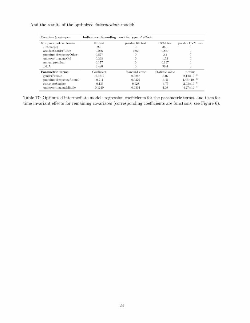
Covariate & category: Indicators depending on the type of effect:

Nonparametric terms: KS test p-value KS test CVM test p-value CVM test(Intercept) 2.5 0 36.1 0acc.death.riderRider 0.266 0.02 0.867 0premium.frequencyOther 0.527 0 2.1 0underwriting.ageOld 0.368 0 1.55 0annual.premium 0.177 0 0.197 0DJIA 3.480 0 99.4 0

Parametric terms: Coefficient Standard error Statistic value p-value

genderFemale -0.0819 0.0267 -3.07 2.14×10−3

premium.frequencyAnnual -0.211 0.0329 -6.41 1.45×10−10

risk.stateSmoker -0.133 0.028 -4.75 2.03×10−6

underwriting.ageMiddle 0.1240 0.0304 4.09 4.27×10−5

Table 17: Optimized intermediate model: regression coefficients for the parametric terms, and tests fortime invariant effects for remaining covariates (corresponding coefficients are functions, see Figure 6).

24