life insurance lapse behavior meetings/2e-life insurance lapse... · life insurance lapse behavior...

LIFE INSURANCE LAPSE BEHAVIOR

Stephen G. Fier** The University of Mississippi

School of Business Administration Holman Hall 338

University, MS 38677 Phone: 662-915-1353

Email: [email protected]

Andre P. Liebenberg The University of Mississippi

School of Business Administration Holman Hall 335

University, MS 38677 Phone: 662-915-5475

Email: [email protected]

**Contact Author

July 2012

LIFE INSURANCE LAPSE BEHAVIOR

ABSTRACT

Life insurance policy lapses are detrimental to issuing insurers when lapses substantially deviate

from insurer expectations. The extant literature has proposed and tested, using macroeconomic

data, several hypotheses regarding lapse determinants. While macroeconomic data are useful in

providing a general test of lapse determinants, the use of aggregate data precludes an analysis of

microeconomic factors that may drive the lapse decision. We develop and test a microeconomic

model of voluntary life insurance lapse behavior and provide some of the first evidence

regarding household factors related to life insurance lapses. Our findings support and extend the

prior evidence regarding lapse determinants. Consistent with the emergency fund hypothesis we

find that voluntary lapses are related to large income shocks, and consistent with the policy

replacement hypothesis we find that the decision to lapse a life insurance policy is directly

related to the purchase of a different life insurance policy. We also find that age is an important

moderating factor in the lapse decision. Changes in income appear to more directly affect the

decision to lapse for younger households, while they are generally unrelated to the lapse decision

for older households.

1

INTRODUCTION

The decision to lapse a life insurance policy can have far-reaching effects on the issuing

insurance company.1 From the insurer’s perspective, excessive policy lapse activity adversely

impacts costs, investment returns, and mortality experience, each of which negatively affects the

financial stability and wellbeing of the insurer (Black and Skipper, 2000).2 Prior literature has

examined lapse determinants from a macroeconomic perspective by explaining time series

variation in national lapse rates in terms of aggregate unemployment rates, interest rates, and

other factors. While these analyses are effective at investigating macroeconomic factors as they

relate to aggregate lapse rates, they are unable to address household-specific factors or events

that drive lapse behavior. Specifically, aggregate data do not lend themselves to explicitly

testing microeconomic hypotheses, nor do they allow for an analysis of important life-cycle

factors that also may be associated with the decision to lapse a policy.

The purpose of this study is to develop and test a microeconomic model of voluntary life

insurance lapse behavior. We use a detailed household-level survey dataset to re-examine some

of the common microeconomic hypotheses associated with life insurance lapse behavior and to

identify household characteristics and life cycle events that affect the lapse decision. More

specifically, we test the emergency fund hypothesis and the policy replacement hypothesis in the

context of life insurance policy lapses using a longitudinal panel dataset. By exploiting the

Health and Retirement Study (HRS) biennial survey from 1998 through 2008, we are able to use

more refined proxies for each of the aforementioned hypotheses to test the relation between

1 Following Kuo et al. (2003), we use the term lapse to encompass both life insurance surrender activity (i.e., electing to receive the cash surrender value that has accumulated in a cash value (whole) life insurance policy in return for the life insurance coverage) and life insurance lapse activity (i.e., cancelling the policy by failing to pay the premium). 2 Carson and Dumm (1999) show that insurer lapse rates are also inversely related to the overall performance of life insurance policies. Similarly, Gatzert, Hoermann, and Schmeiser (2009) provide evidence that secondary market purchases of life insurance impacts expected lapse and surrender rates which can negatively impact insurer profits.

2

important household-specific factors and the decision to lapse a life insurance policy.

Furthermore, our examination of the lapse decision by age group allows for a more complete

analysis of the effect of life cycle factors on the lapse decision.

Our results provide evidence in favor of both the emergency fund hypothesis and the

policy replacement hypothesis. Specifically, we find that the probability of voluntarily lapsing a

policy is higher for households that suffered a large negative income shock and that reported

greater amounts of household debt. Our results also suggest that the decision to lapse a life

insurance policy is directly related to the purchase of a different life insurance policy, consistent

with the policy replacement hypothesis. The determinants of the lapse decision are moderated

by age. Changes in income appear to more directly affect the decision to lapse for younger

households, while they are generally unrelated to the lapse decision for older households.

Our results are both statistically and economically significant. For example, with respect

to the emergency fund hypothesis proxies, we find that, ceteris paribus, households that suffered

substantial negative income and net worth shocks are roughly 25 percent more likely to lapse a

policy than are other households. With respect to the policy replacement hypothesis proxy, we

find that households that purchase a new life insurance policy are roughly 4 times more likely to

lapse a policy than are other households. Additionally, households in the youngest age quartile

are almost twice as likely to lapse as are older households.

The remainder of this study is organized as follows. In the next section, we discuss the

life insurance lapse literature, with a particular focus on the factors related to the decision to

lapse a policy. Next, we provide a discussion of the data, methodology, and variables employed

3

to test each of the aforementioned hypotheses. A discussion regarding the results of the study

and implications of the results is provided, followed by the conclusion.

LAPSE LITERATURE

Unlike the insurer that originates the life insurance policy contract, the owner of a life insurance

policy has the option to lapse or surrender the life insurance policy at any point in time.3 This

ability to readily lapse a policy can adversely impact the financial solvency of an insurer if the

lapse activity is greater than expected and/or if a large proportion of policyholders decide to

lapse their policies at the same time (analogous to a run on a bank). In such instances, insurer

operations can be impaired in a number of different ways. First, insurers typically incur the

greatest proportion of policy expenses through the acquisition of new business (e.g.,

commissions, policy issuance costs, administrative costs, etc.), where it can often take years

before the insurer fully recoups those costs. If a policyowner lapses a policy before those costs

can be recouped, the insurer must find a way to recover those costs. Second, policy lapses and

surrenders could result in a situation where the insurer must liquidate high-yielding investments

in order to satisfy policyholder requests for surrender values.4 Third, excessive policy lapsation

can influence pricing when lapses are greater than expected or when they cause actual mortality

rates experienced by the insurer to deviate from expected mortality rates (e.g., Doherty and

Singer, 2002; Gatzert, Hoermann, and Schmeiser, 2009).

Researchers have suggested a number of explanations for lapse behavior, including the

emergency fund hypothesis (EFH), the interest rate hypothesis (IRH), and the policy replacement

3 Smith (1982) and Walden (1985) discuss the value of various options contained within life insurance policies, including the option to surrender a life insurance policy. 4 This potential problem associated with policy surrender assumes that the policy is a whole life insurance policy and that the cash value that has accumulated within the policy (if any) exceeds surrender charges.

4

hypothesis (PRH). The EFH (Linton, 1932; Outreville, 1990; Kuo, Tsai and Chen, 2003; Kim,

2005) argues that individuals will be more likely to lapse a life insurance policy when faced with

economic hardship. This decision could be due to (1) a desire to use the funds that would

otherwise go to premium payments for other important needs or (2) a desire to take advantage of

any cash value that has accrued within the policy to cover various household expenses. The IRH

(Schott, 1971; Pesando, 1974; Kuo, Tsai, and Chen, 2003) states that policyowners may be

willing to remove funds from a life insurance policy (either by way of loan or surrender) in order

to take advantage of higher market rates.5 Finally, the PRH (Outreville, 1990; Russell, 1997;

Carson and Forster, 2000) states that policy lapses may occur simply because the policyholder

has identified a more attractive policy with better terms or rates. Under this hypothesis, one

anticipates a positive relationship between new life insurance business and policy lapses, as

individuals allow a policy to lapse for the explicit purpose of purchasing a new life insurance

policy.

Over the past twenty years, empirical investigations into the motives for policy lapses

have generally reported evidence supporting the EFH and have also found evidence consistent

with the PRH. As alluded to earlier, these studies typically are conducted using aggregate

(macroeconomic) data to test the different hypotheses. For instance, Dar and Dodds (1989) use

aggregate data on endowment life insurance policies written by British life insurers from 1952

through 1985. Consistent with the EFH, they find that unemployment is directly related to the

policy surrender decision Similarly, Outreville (1990) utilizes country-level data (both for the

United States and for Canada) for the period 1966 through 1979 to examine policy lapses while

5 For instance, Carson and Hoyt (1992) show that policyowners were more likely to take a loan on a whole life policy when market rates exceeded the rate to borrow the cash value (prior to the use of floating policy loan interest rates).

5

Russell (1997) uses U.S. state-specific economic variables to identify important factors related to

the decision to surrender a life insurance policy. In each of these studies, there is evidence in

favor of both the EFH and the PRH. Additional support for the EFH is presented by Kim (2005)

and Jiang (2010) using macroeconomic data from Korea and the U.S., respectively. Kuo, Tsai

and Chen (2003) test the relative importance of the EFH and the IRH. Using aggregate data

from the American Council of Life Insurers (ACLI) for the period 1951-1998, Kuo et al. (2003)

report evidence consistent with the EFH and the IRH, but they also find that the impact of

interest rates on lapse behavior is of greater economic importance. Finally, Kiesenbauer (2011)

uses company-level German life insurer data and finds limited support for the EFH.

Although much of the empirical research that has examined the EFH and PRH with

respect to lapses has relied on macroeconomic data, some recent studies have used

microeconomic data. For example, Liebenberg, Carson and Dumm (2012) employ household-

level data from the Survey of Consumer Finances (SCF) longitudinal panel dataset (for the years

of 1983 and 1989) to test the factors related to both the demand for life insurance and the

decision to “drop” life insurance. Among their findings, the authors report that decisions

regarding life insurance holdings are significantly related to whether one of the spouses in a

household recently became unemployed, consistent with the EFH.6 They also report evidence

consistent with the PRH.

6 While Liebenberg, Carson and Dumm (2011) do examine the decision to “drop” a life insurance policy, their definition of a “dropped” policy does not focus specifically on those households that decide to completely lapse/surrender a policy. In particular, the authors define dropped coverage as: “…equal to one for households that decreased the amount of, or completely dropped, their term (whole life) insurance…” As such, the analysis conducted by Liebenberg et al. (2011) does not explicitly test the reason for lapses, but rather, investigates the factors associated with changes in overall life insurance holdings (i.e., both lapses and coverage reductions).

6

DATA AND METHODOLOGY

While much of the literature provides fairly consistent support for the EFH, it should be

reiterated that the majority of the empirical evidence is provided through the use of aggregate

(macroeconomic) data. This is an important point, given that the EFH and PRH are generally

viewed as microeconomic hypotheses and that aggregate data do not lend themselves to directly

testing microeconomic hypotheses. For example, in the policy loan literature, using household-

level data, Liebenberg, Carson, and Hoyt (2010) find support for the EFH while other

researchers had failed to find such evidence. The authors argue that this difference may be due

to the fact that aggregate data had been used in prior studies rather than potentially more

informative microeconomic data. Accordingly, we use household-level data to test the EFH and

PRH while controlling for life-cycle factors that are also expected to influence the lapse

decision.7

In order to more fully explore the EFH and PRH, we use data collected through the

University of Michigan Health and Retirement Study (HRS). The HRS is longitudinal panel

study with a focus on Americans over the age of 50. The survey is conducted on a biennial basis

and includes questions regarding respondents’ employment, financial, and health status. The

survey includes questions that explicitly address household-specific life insurance holdings and

lapses.

While prior literature (e.g., Liebenberg et al. 2012) has used the Survey of Consumer

Finances (SCF) to examine changes in life insurance holdings, the HRS data offers some

7 Due to the nature of the data, we are unable to test the interest rate hypothesis (IRH). Such a test would generally require the use of either (1) macroeconomic factors and/or (2) additional information regarding the specific characteristics of the life insurance policy. Since the HRS data only provides limited information regarding the policies held by the respondents and because we are interested in evaluating the household-level factors, we exclude the IRH from the analysis.

7

advantages over the SCF. Most importantly, the HRS questionnaire specifically asks

respondents whether they lapsed a policy while the SCF survey does not. Although the SCF data

provides information on life insurance policies, one must infer whether changes to a household’s

life insurance holdings were explicitly due to a lapse and whether or not such a change was

voluntary. So, while the SCF data allowed Liebenberg et al. (2012) to examine reductions in the

net amount at risk, we are able to more accurately determine whether or not a lapse occurred and

when it occurred. Additionally, the HRS is a longitudinal survey that has been conducted

biennially since 1992, whereas the SCF is primarily a cross-sectional survey that offers panel

data for only two periods (1983-1989 and 2007-2009). These features of the HRS data enable us

to directly test determinants of the life insurance lapse decision at the household level.

To construct our dataset, we use data from the 1996, 1998, 2000, 2002, 2004, 2006, and

2008 waves of the HRS.8 The total number of households contained in the dataset without

further screens is 17,151. Households are removed from the sample if they have missing values

for any of the independent variables that are discussed below or if there are insufficient data for

the calculation of changes in net income and changes in net worth. After applying these screens

the final sample consists of 14,673 unique households that account for 59,675 household-year

observations.9

In order to determine if a household lapsed a life insurance policy since the previous

survey, we focus on the following question in each biennial survey:

8 We exclude 1992 and 1994 as the HRS survey did not ask lapse-specific questions in those years. 9 The majority of households dropped from the sample are those that did not report household-specific income or that were new entrants into the sample and did not have historical data required for calculation of the change variables.

8

Question: In the last two years, have you allowed any life insurance policies to lapse or have any

been cancelled?

Respondents that answered in the affirmative were initially classified as having lapsed a

policy. An additional question in the survey allows us to further identify whether the lapse was

initiated by the respondent or by some other party. Specifically, the survey asks respondents the

following question:

Question: Was this lapse or cancellation something you chose to do, or was it done by the

provider, your employer, or someone else?

This additional question allows us to classify lapses as voluntary and involuntary. Since

the purpose of our analysis is to test household-specific lapse determinants all involuntary lapses

are removed from the sample.10

The decision to lapse a life insurance policy ( , ) is assumed to be the outcome of a

latent (unobserved) variable, ,∗ , where ,

∗ is a linear function of household factors that are

hypothesized to be associated with the lapse decision. This relation is given in Equation (1) as:

,∗

, , (1)

Where , is a coefficient vector (for household i in year t) that consists of lapse

determinants and , is a random error term. The observed decision to lapse a life insurance

policy for a given household in a given year is presented in Equation (2) as:

10 Additional variations of the models were estimated when including (1) involuntary lapse observations as “non-lapse” events and (2) involuntary lapses and classifying them as lapse events. The results from these specifications are discussed below.

9

,

1 if L ,∗ 0

0 otherwise (2)

Under the assumption that the random error term ( , in Equation (1) has an expected

value of zero and is distributed logistically with Var( , ) = , the general form of the logistic

regression model is given as:

Pr 1|

exp1 exp

(3)

The coefficient vector includes variables that specifically test the EFH and PRH as well

as a set of control variables that capture the effect of life-cycle factors and other characteristics

on the lapse decision. The relationship between the observed lapse decision and its determinants

can be functionally represented as:

, = f (Emergency Fund Hypothesis Variables, Policy Replacement Hypothesis Variables, Life-Cycle Variables, Control Variables).

(4)

Yearly fixed effects are included in each model and standard errors are clustered at the

household level (Petersen, 2009). Below we further discuss and describe each of the variables

included in the model.

Emergency Fund Hypothesis Variables

Unemployment. Prior tests of the EFH proxy for the effect of financial hardship on lapses by

using aggregate unemployment rates (e.g., Dar and Dodds, 1989; Outreville, 1990; Kuo et al.,

2003). We directly capture the effect of recent household unemployment by using a binary

variable set equal to 1 if the respondent or spouse reports a work status of “unemployed” after

reporting a non-unemployed work status in the previous survey (NewUnemploy). Consistent

10

with the EFH, we expect a positive and significant relation between unemployment and the

decision to lapse a policy.

Income/Wealth Shocks. Similar to Liebenberg et al. (2010) we also test the EFH by examining

the relation between the lapse decision and negative shocks to household income or net worth11.

Households that experienced the greatest reduction in income or wealth should be more likely

than other households to lapse a policy. Households that experience negative changes in income

(wealth) are placed into quartiles based on the size of the change. Households in the first quartile

have the largest negative changes, while households in the fourth quartile have the smallest

negative changes or experienced positive changes. Using the fourth quartile as the numeraire, the

EFH predicts a positive relation between the lapse decision and the first three quartiles of income

shocks (NegInc1, NegInc2, and NegInc3) and wealth shocks (NegNW1, NegNW2, and

NegNW3).12

Policy Replacement Hypothesis Variable

New Life Insurance. The policy replacement hypothesis posits that consumers surrender policies

with the intent of replacing the original policy with one that has better terms or a lower price

(Russell, 1997). Consistent with the PRH, Outreville (1990) and Russell (1997) find that policy

lapses and surrenders are positively related to new life insurance purchases. We test the PRH by

11 We calculate net worth as household assets minus household liabilities. Household assets include: (1) the net value of stocks, mutual funds, and investment funds; (2) the value of checking, savings, or money market accounts; (3) the value of CDs, government savings bonds, and Treasury bills; (4) the net value of vehicles; (5) the net value of businesses; (6) the net value of real estate; (7) the net value of bonds and bond funds; (8) the net value of IRAs and Keogh accounts; (9) the value of the primary residence; and (10) the value of all other savings. Liabilities are calculated as the sum of: (1) the value of the mortgage on the primary residence; (2) value of other loans on the home; and (3) the value of all other debt. 12 It should be noted that this decision to lapse a policy following a reduction of income could be attributed to either (1) the household needing funds contained within the policy to cover expenses or (2) the household being unable to pay the premium or unwilling to allocate a portion of current household funds to continue paying premiums. Unfortunately, the data do not allow us to distinguish between the two aforementioned reasons.

11

including a binary variable denoting the purchase of a new life insurance policy since the

previous survey (NewLife).13

Life Cycle Variables

The life cycle literature suggests that significant changes in an individual’s life impact the

demand for insurance (e.g., Liebenberg et al., 2012). We therefore include variables that capture

several major life events. We discuss each of the life cycle variables below:

Age. Prior researchers have found a non-linear effect between age and life insurance demand

(Lin and Grace, 2007, Liebenberg et al. 2012). We capture the potential non-linear impact of age

on the lapse decision in two ways. First, we include the age of the respondent at the conclusion

of a given year’s survey (Age) as well as its squared value (Age_Sq). Second, we place

households into quartiles based on the age of the household’s primary respondent (Age_46-62,

Age_63-68, and Age_69-76).

Recently Divorced. A binary variable denoting whether the respondent is recently divorced is

included in each model (NewDivorced). A recent divorce could require the divorcee to become

more reliant on their own income, which could result in financial hardship. Alternatively, a

recent divorce could lead the policyowner to lapse a policy if the respondent is the policyowner

on a policy written on the life of the ex-spouse.

Recently Retired. We also include a binary variable denoting if the respondent is recently retired

(NewRetired). Liebenberg et al. (2012) find a positive relation between recent retirement and

the decision to drop term life insurance coverage. The authors argue the relationship may be

explained as either the result of (1) the loss of employer-sponsored life insurance or (2) the

13 Individuals are identified as having purchased a new life insurance policy since the previous HRS survey based on the following survey question: “In the last two years, have you obtained any new life insurance policies?”

12

substitutability of retirement income for life insurance. An advantage of our dataset is that we

are able to differentiate between voluntary and involuntary lapse/cancellation.

Recent Widow. Following the death of a spouse, the remaining spouse may allow an outstanding

policy to lapse as the financial benefit derived from the policy may no longer be required. To

capture this effect, we include an indicator variable equal to one if the respondent was recently

widowed, and zero otherwise (NewWidowed).

Control Variables

Beyond the primary variables of interest, we also include control variables that have been shown

to relate to the lapse decision.14

Income and Net Worth. While we test the EFH by estimating the effect of negative income and

wealth shocks on the lapse decision, we also control for the level of household income and

wealth using the natural logarithm of reported household income (Income) and net worth

(NetWorth).

Debt. Following Frees and Sun (2012) and Lin and Grace (2007) we control for the household-

level of debt in the models using the natural logarithm of total debt (Debt).

Liquidity. Hau (2000) finds that the liquidity of asset holdings is significantly related to the life

insurance holding decision. We therefore include in our models a measure of asset liquidity,

calculated as the sum of liquid assets scaled by total assets (Liquidity).15

14 In addition to the control variables included in the model, we also considered the inclusion of a bequest variable. The HRS survey asks respondents the following question: “Including property and other valuables that you might own, what are the chances that you (and your [husband/wife/partner]) would leave an inheritance totaling $50,000 or more / $100,000 or more / $10,000 or more?” Because a small proportion of the total sample answers this question, it greatly reduces the overall size of the sample. However, we re-estimated each of the models using a variety of bequest proxies and found no significant relation between the bequest proxies and the decision to lapse (while the other variables remained qualitatively similar). As such, we do not report the results of the models with the inclusion of the bequest variables.

13

Children. Prior studies indicate that there is often a statistical relation between family size, or the

number of children in the household, and life insurance demand (e.g., Burnett and Palmer, 1984;

Browne and Kim, 1993). Accordingly, we include a variable denoting the total number of

children reported by the respondent (Kids).

Employment Status. Liebenberg et al. (2012) find that working households are less likely to drop

their whole life insurance. We therefore account for current employment status by including an

indicator variable equal to one if at least one spouse in the household is currently employed

(Working).

Education. Browne and Kim (1993), Truett and Truett (1990), and Li et al. (2007) find a positive

relation between education and life insurance demand. We include a binary variable denoting if

either spouse in the household has earned a college degree to control for the effect of household-

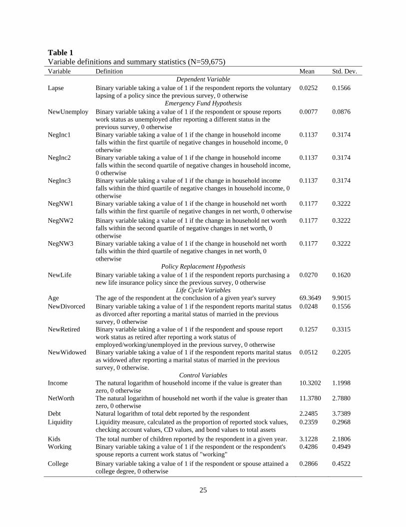
level education on the lapse decision (College). Variable definitions and summary statistics are

provided in Table 1.

[Insert Table 1 here]

RESULTS

Univariate Comparison

In order to evaluate the impact that household factors have on the decision to lapse a life

insurance policy, we first perform a univariate comparison of the independent variables across

those households that lapsed a policy and those that did not lapse a policy. Results, reported in

Table 2, provide support for both the EFH and the PRH. Consistent with the EFH, households

that suffered the largest shock to income (NegInc1 and NegInc2) or net worth (NegNW1) were

15Liquid assets include: (1) the net value of stocks, mutual funds, and investment funds; (2) the value of checking, savings, or money market accounts; (3) the value of CDs, government savings bonds, and Treasury bills; and (4) the net value of bonds and bond funds.

14

more likely than others to lapse a life insurance policy. Consistent with the PRH, approximately

13.7 percent of households that lapsed a policy also purchased a new life insurance policy

(NewLife), compared to roughly 2.4 percent for those households that did not lapse.


The life cycle results reported in Table 2 suggest a univariate relation between the lapse decision

and measures of age and recent retirement. In general, households that lapse tend to be

significant younger than those that do not lapse. However, the age-lapse relation appears to be

non-linear as households in the first two age quartiles are more likely to lapse while those in the

third and fourth age quartiles are less likely to lapse. Recent retirees are also more likely to lapse

than are other households. Finally, univariate differences in lapse behavior are also evident for

several of our control variables. We next utilize a multivariate framework to more carefully test

the determinants of the lapse decision.

Multivariate Analysis

We use logistic regression to estimate the relation between the lapse decision and various

household-specific factors in a multivariate setting. Given the importance of age in life insurance

demand, and the apparent non-linear age-lapse relation identified in Table 2, we estimate two

forms of the basic model. The first specification captures the potentially non-linear age-lapse

relation by including a continuous age variable as well as a squared age variable (Lin and Grace,

2007). The second specification models the non-linear age-lapse relation using indicator

variables for the three youngest age quartiles.

Results for the two model specifications are reported in Table 3. In general, we find that

our results are fairly consistent across both specifications. Focusing first on the two hypotheses

15

of interest, we find a positive and statistically significant relation between both NegInc1 and

NegInc2 and the lapse decision. This finding supports the notion that households that experience

the largest negative shocks to income are more likely to lapse a life insurance policy than are

other households.16We also report a positive and statistically significant relation between a large

negative shock to net worth (NegNW1) and the lapse decision to lapse, which is again consistent

with the EFH. While negative shocks to income and net worth are associated with the lapse

decision, we do not find evidence linking recent unemployment (NewUnemploy) to policy lapses.

We believe that this is a result of the fact that we focus solely on voluntary lapses rather than all

lapses. By omitting involuntary lapses, we remove instances where a household would appear to

have lapsed a policy when in reality the household more accurately lost an employee benefit as

part of employment termination.17 Taken together, these results support the EFH as one

explanation for life insurance policy lapses.


In addition to finding strong evidence in favor of the EFH, we also find support for the

PRH. Our results suggest a positive and significant relation between policy lapses and the

purchase of a new life insurance policy (NewLife). These findings imply that households that

lapse life insurance policies are likely to purchase another life insurance policy. In other words,

16 Post-estimation, we test to determine if the coefficient on NegInc1 and the coefficient on NegInc2 statistically differ both for Model 1 and Model 2. We fail to reject the null hypothesis that the coefficients on NegInc1 and NegInc2 differ significantly. We also test to determine if the coefficients on NegInc1 and NegInc2 differ from the coefficient on NegInc3. We reject the null hypothesis that NegInc1 and NegInc2 have coefficients that are statistically equivalent to the coefficient on NegInc3. 17 Additional variations of the models were estimated when including (1) involuntary lapse observations as “non-lapse” events and (2) involuntary lapses and classifying them as lapse events. The (unreported) results are qualitatively similar for all independent variables except the unemployment variable (NewUnemploy). When classifying involuntary lapses as voluntary lapses, the coefficient on the unemployment variable is positive and statistically significant. This result is not surprising, as involuntary lapses are often the result of unemployment or employers removing life insurance as an employee benefit.

16

households may allow policies to lapse for the purpose of replacing the policy with another

policy that has better terms or a lower price. This finding is consistent with a recent Life

Insurance Market Research Association (LIMRA) study that reports that 13 percent of survey

respondents indicated that they purchased life insurance to replace another life insurance policy

(LIMRA, 2011).

The results in Table 3 also establish a link between the decision to lapse and important

life-cycle factors. First, we find that age plays an important role in the lapse decision. The

results from Model 1 suggest a quadratic relation between age and lapses, whereby the likelihood

of policy lapsation increases over time and then subsequently declines. Similarly, in model 2, we

find that the youngest households (i.e., those in the first three age quartiles) are more likely to

lapse a life insurance policy than are the oldest households in the sample (i.e., those in the fourth

quartile). The importance of age as a factor in the lapse decision is also observable through an

examination of the size of the coefficients on each of the age quartile variables in Model 2.

Specifically, there is a clear downward trend in the size of the coefficient moving from the

youngest households to the oldest households. We find that two life events are also associated

with the lapse decision. Specifically, we find that recently retired households (NewRetired) and

recently widowed households (NewWidowed) are more likely to lapse policies than are other

households. Beyond the results for our variables of interest, we also find that greater household

debt (Debt) and educational attainment are positively related to the lapse decision18

In general, the results discussed above suggest that (1) households are more likely to

lapse a life insurance policy given increasing financial hardship (in support of the EFH), (2)

18 We re-estimated each of the models and replaced the Kids variable with a binary variable that denotes instances where a respondent reported the addition of a new child to the household. The results from these additional specifications do not differ qualitatively from those presented in Table 3, and are thus are not presented.

17

households are more likely to lapse policies when, during the same time period, purchasing a

new life insurance policy (in support of the PRH), and (3) several life-cycle factors, including

age, retirement, and the death of a spouse significantly relate to the lapse decision. However,

prior literature generally contends that decision-making differs across various age groups. For

instance, Truett and Truett (1990) find a positive and significant relation between age and life

insurance demand while Lin and Grace (2007) report that older individuals are less likely to use

life insurance to protect against financial vulnerability than are younger individuals. We

therefore further evaluate the determinants of the lapse decision conditional on policyholder age.

Lapse Behavior by Age

In the previous section, we provided support for the EFH and PRH and found that significant life

events can impact the lapse decision. In this section, we further explore the relation between the

decision to lapse a life insurance policy and age. We investigate this relation by separating the

sample into groups based on the respondent’s attained age in a given survey year. Specifically,

we separate the sample into distinct groups based on age quartiles, where households are placed

into quartiles based on the age of the household’s primary respondent.19 The models are then

estimated for each of these age groups, using the same variables included in the original

specifications presented in Table 3.

Prior to examining the multivariate relationships across the age quartiles, we provide a

univariate comparison of the variables in Table 4. The univariate analysis compares those

individuals that are in the first two age quartiles (Age_46-68) to the older sample households.

We report significant differences between the first two quartiles and the last two quartiles across

19 It should be noted that this method of partitioning the sample allows for a household to move across quartiles over time as the household respondent ages.

18

the majority of variables. These results suggest that age might be a moderating factor in the

relation between household characteristics and the lapse decision and support the further

examination of lapse behavior by age quartile.


The results obtained from the multivariate models based on age quartiles are presented in

Table 5.20 In general, the results suggest that lapse determinants do differ across age quartiles.

Most notably, we find that support for the EFH is limited to younger sample households. While

income and wealth shocks are significant predictors of lapses for younger households, they are

not related to the lapse decision for older households.


The coefficient on NewLife is positive and significant in all Table 5 model specifications.

Regardless of age, the results indicate that life insurance policy replacement is a consistent

reason for life insurance policy lapses. Not surprisingly, results across the life cycle variables

differ across the various age quartiles. The coefficient on NewDivorced is positive and

significant only for the youngest households in the sample, while recent retirement (NewRetired)

is an important consideration for those households in the first two quartiles. The recent death of a

spouse (NewWidowed) is also an important life-cycle factor, but it is only a significant factor for

older households in the third quartile.

The results reported in both Tables 3 and 5 all generally support the EFH and the PRH.

However, as shown in Table 5, the factors directly attributable to the decision to lapse vary

20 It should be noted that the NewUnemploy variable is omitted from the Quartile 3 and Quartile 4 results, while the NewDivorced variable is omitted from the Quartile 4 results. These variables are omitted from the model as they perfectly predict the lapse outcome.

19

across age groups, with age moderating the effect of negative income and wealth shocks on the

lapse decision. Moreover, our results indicate that while financial hardship and policy

replacement both impact the decision to lapse a policy, life-cycle factors play an important role

in the lapse decision-making process.

Probabilistic Interpretation of Results

The results reported in Tables 3 and 5 both lend statistical support for the EFH and the PRH.

However, it is also important to understand the economic significance of our findings. Table 6

reports a probabilistic interpretation of the results reported in Table 4. Specifically, the table

reports the probability of lapse behavior for each binary variable at values of 1 and 0, holding all

other independent variables at their means, as well as marginal effects. First, we find that, ceteris

paribus, households that suffered substantial negative income shocks (NegInc1 and NegInc2) are

roughly 25 percent more likely to lapse a policy than are other households. Similarly, households

that suffered substantial negative wealth shocks (NegNW1) are roughly 26 percent more likely

than other households to lapse a policy. Second, households that purchase a new life insurance

policy (NewLife) are roughly 4 times more likely to lapse a policy than are households that do

not purchase a new policy, with purchasers of new policies exhibiting a 9.99 percent chance of a

lapse compared to only a 2.04 percent chance of a lapse for those that do not purchase a new

policy. Our life-cycle results are also economically significant. Recently retired households are

roughly 25 percent more likely to lapse than other households and recently widowed individuals

are almost 30 percent more likely to lapse. Further, the probability estimates for Model 2 indicate

that households in the youngest age quartile are almost twice as likely to lapse as are older

households.


20

Overall, our results suggest that household-specific factors are statistically and

economically significant predictors of the decision to lapse a life insurance policy.

CONCLUSIONS

The life insurance policy lapse literature typically examines the decision to lapse from a

macroeconomic framework and finds evidence consistent with the emergency fund, policy

replacement and interest rate hypotheses (e.g., Outreville, 1990; Russell, 1997; Kim, 2005).

However, the majority of these studies have been conducted using macroeconomic data rather

than microeconomic (household) data. The use of aggregate data can have the unintended effect

of removing important variation that is necessary in order to test hypotheses that have a

microeconomic basis such as the emergency fund hypothesis and the policy replacement

hypothesis (e.g., Liebenberg, Carson and Hoyt, 2010). Given the potential impact that policy

lapses and surrenders can have on the overall performance of life insurance companies (e.g.,

Carson and Dumm, 1999; Black and Skipper, 2000; Gatzert, Hoermann, and Schmeiser, 2009),

we re-examine the decision to lapse life insurance policies using household-level data.

Using the Health and Retirement Study (HRS), we are able to directly test the emergency

fund hypothesis and the policy replacement hypothesis. Additionally, the dataset provides us

with insight regarding household characteristics that can be exploited to test the relation between

various life-cycle factors such as divorce and retirement and the decision to lapse a policy.

Overall, the results provide support for both the emergency fund hypothesis as well as the policy

replacement hypothesis. In particular, we find that households that experience large negative

shocks to income and net worth are more likely to lapse a policy. We also find recent retirement

and the recent death of a spouse is directly related to the decision to lapse a life insurance policy.

21

Beyond the initial findings, our results suggest that the decision to lapse a policy is also strongly

dependent on the policyowner’s age. In particular, while negative shocks to income appear to be

of particular importance for younger households, there is no evidence linking financial shocks to

lapse activity for older households.

The results of this study are important for a number of reasons. First, as noted

previously, household-level data may provide more useful information than its aggregate-level

counterpart, allowing for a more complete examination of the hypotheses discussed above.

Second, the use of a longitudinal panel dataset allows us to track households over a twelve year

time span, which creates the opportunity to examine important household changes that may be

directly related to the lapse decision. The same characteristics of the data that allow us to track

the financial condition of each household over time also allows us to account for a variety of life-

cycle factors that we show are related to the decision to lapse. Finally, the results in this study

illustrate the importance of age as a moderating factor in the lapse decision.

22

References

Black, Kenneth Jr. and Harold J. Skipper, 2000, Life and Health Insurance (13th Edition), New Jersey: Prentice-Hall, Inc.

Browne, Mark J. and Kihong Kim, 1993, “An International Analysis of Life Insurance Demand,” Journal of Risk and Insurance, 60(4): 616-634.

Burnett, John J. and Bruce A. Palmer, 1984, “Examining Life Insurance Ownership Through Demographic and Psychographic Characteristics,” Journal of Risk and Insurance, 51(3): 453-467.

Carson, James M. and Randy E. Dumm, 1999, “Insurance Company-Level Determinants of Life Insurance Policy Performance,” Journal of Insurance Regulation, 18: 195-206.

Carson, James M. and Mark D. Forster, 2000, “Suitability and Life Insurance Policy Replacement,” Journal of Insurance Regulation, 18(4): 427-447.

Carson, James M. and Robert E. Hoyt, 1992, “An Econometric Analysis of the Demand for Life Insurance Policy Loans,” Journal of Risk and Insurance, 59: 239-251.

Dar, A. and J.C. Dodds, 1989, “Interest Rates, the Emergency Fund Hypothesis and Saving through Endowment Policies: Some Empirical Evidence for the U.K.,” Journal of Risk and Insurance, 56(3): 415-433.

Doherty, Neil A. and Hal J. Singer, 2002, “The Benefits of a Secondary Market for Life Insurance Policies,” Wharton Financial Institutions Center Working Paper 02-41.

Frees, Edward W. (Jed) and Yunjie (Winnie) Sun, 2010, “Household Life Insurance Demand: A Multivariate Two-Part Model,” North American Actuarial Journal, 14(3): 338-354.

Gatzert, Nadine, Gudrun Hoermann, and Hato Schmeiser, 2009, “The Impact of the Secondary Market on Life Insurers’ Surrender Profits,” Journal of Risk and Insurance, 76(4): 887-908.

Hau, Arthur, 2000, “Liquidity, Estate Liquidation, Charitable Motives, and Life Insurance Demand by Retired Singles,” Journal of Risk and Insurance, 67(1): 123-141.

Jiang, Shi-jie, 2010, “Voluntary Termination of Life Insurance Policies: Evidence from the U.S. Market,” North American Actuarial Journal, 14(4): 369-380.

Kiesenbauer, Dieter, 2011, “Main Determinants of Lapse in the German Life Insurance Industry,” Preprint Series: 2011-03, Working Paper, Accessed on November 17, 2011 from http://www.uni-ulm.de/fileadmin/website_uni_ulm/mawi/forschung/PreprintServer/2011/Lapse.pdf

23

Kim, Changki, 2005, “Modeling Surrender and Lapse Rates with Economic Variables,” North American Actuarial Journal, 9(4): 56-70.

Kuo, Weiyu, Chenghsien Tsai, and Wei-Kuang Chen, 2003, “An Empirical Study on the Lapse Rate: The Cointegration Approach,” Journal of Risk and Insurance, 70(3): 489-508.

Li, Donghui, Fariborz Moshirian, Pascal Nguyen, and Timothy Wee, 2007, “The Demand for Life Insurance in OECD Countries,” Journal of Risk and Insurance, 74(3): 637-652.

Liebenberg, Andre P., James M. Carson and Robert E. Hoyt, 2010, “The Demand for Life Insurance Policy Loans,” The Journal of Risk and Insurance, 77(3): 651-666.

Liebenberg, Andre P., James M. Carson and Randy E. Dumm, 2012, A Dynamic Analysis of the Demand for Life Insurance. Journal of Risk and Insurance. doi: 10.1111/j.1539-6975.2011.01454.x

LIMRA, 2011, “2011 LIMRA Buyer / Nonbuyer Study,” Accessed on December 12, 2011 from http://www.soa.org/files/pdf/2011-chicago-annual-mtg-145.pdf.

Lin, Yijia and Martin F. Grace, 2007, “Household Life Cycle Protection: Life Insurance Holdings, Financial Vulnerability, and Portfolio Implications,” Journal of Risk and Insurance, 74(1): 141-173.

Outreville, J. Francois, 1990, “Whole-Life Insurance Lapse Rates and the Emergency Fund Hypothesis,” Insurance: Mathematics and Economics, 9: 249-255.

Pesando, James E., 1974, “The Interest Sensitivity of the Flow of Funds Through Life Insurance Companies: An Econometric Analysis,” Journal of Finance, 29(4): 1105-1121.

Petersen, Mitchell A., 2009, “Estimating Standard Errors in Finance Panel Data Sets: Comparing Approaches,” Review of Financial Studies, 22(1): 435-480.

Russell, David T., 1997, “An Empirical Analysis of Life Insurance Policyholder Surrender Activity,” Dissertation.

Satterthwaite, F.E., 1946, “An Approximate Distribution of Estimates of Variance Components,” Biometrics Bulletin, 2: 110-114.

Schott, Francis H., 1971, “Disintermediation through Policy Loans at Life Insurance Companies,” Journal of Finance, 26(3): 719-729.

Smith, Michael L., 1982, “The Life Insurance Policy as an Options Package,” Journal of Risk and Insurance, 49(4): 583-601.

Truett, Dale B. and Lila J. Truett, 1990, “The Demand for Life Insurance in Mexico and the United States: A Comparative Study,” Journal of Risk and Insurance, 57(2): 321-328.

24

Walden, Michael L., 1985, “The Whole Life Insurance Policy as an Options Package: An Empirical Investigation,” Journal of Risk and Insurance, 52(1): 44-58.

25

Table 1 Variable definitions and summary statistics (N=59,675) Variable Definition Mean Std. Dev.

Dependent Variable Lapse Binary variable taking a value of 1 if the respondent reports the voluntary

lapsing of a policy since the previous survey, 0 otherwise 0.0252 0.1566

Emergency Fund Hypothesis NewUnemploy Binary variable taking a value of 1 if the respondent or spouse reports

work status as unemployed after reporting a different status in the previous survey, 0 otherwise

0.0077 0.0876

NegInc1 Binary variable taking a value of 1 if the change in household income falls within the first quartile of negative changes in household income, 0 otherwise

0.1137 0.3174

NegInc2 Binary variable taking a value of 1 if the change in household income falls within the second quartile of negative changes in household income, 0 otherwise

0.1137 0.3174

NegInc3 Binary variable taking a value of 1 if the change in household income falls within the third quartile of negative changes in household income, 0 otherwise

0.1137 0.3174

NegNW1 Binary variable taking a value of 1 if the change in household net worth falls within the first quartile of negative changes in net worth, 0 otherwise

0.1177 0.3222

NegNW2 Binary variable taking a value of 1 if the change in household net worth falls within the second quartile of negative changes in net worth, 0 otherwise

0.1177 0.3222

NegNW3 Binary variable taking a value of 1 if the change in household net worth falls within the third quartile of negative changes in net worth, 0 otherwise

0.1177 0.3222

Policy Replacement Hypothesis NewLife Binary variable taking a value of 1 if the respondent reports purchasing a

new life insurance policy since the previous survey, 0 otherwise 0.0270 0.1620

Life Cycle Variables Age The age of the respondent at the conclusion of a given year's survey 69.3649 9.9015 NewDivorced Binary variable taking a value of 1 if the respondent reports marital status

as divorced after reporting a marital status of married in the previous survey, 0 otherwise

0.0248 0.1556

NewRetired Binary variable taking a value of 1 if the respondent and spouse report work status as retired after reporting a work status of employed/working/unemployed in the previous survey, 0 otherwise

0.1257 0.3315

NewWidowed Binary variable taking a value of 1 if the respondent reports marital status as widowed after reporting a marital status of married in the previous survey, 0 otherwise.

0.0512 0.2205

Control Variables Income The natural logarithm of household income if the value is greater than

zero, 0 otherwise 10.3202 1.1998

NetWorth The natural logarithm of household net worth if the value is greater than zero, 0 otherwise

11.3780 2.7880

Debt Natural logarithm of total debt reported by the respondent 2.2485 3.7389 Liquidity Liquidity measure, calculated as the proportion of reported stock values,

checking account values, CD values, and bond values to total assets 0.2359 0.2968

Kids The total number of children reported by the respondent in a given year. 3.1228 2.1806 Working Binary variable taking a value of 1 if the respondent or the respondent's

spouse reports a current work status of "working" 0.4286 0.4949

College Binary variable taking a value of 1 if the respondent or spouse attained a college degree, 0 otherwise

0.2866 0.4522

26

Table 2 Univariate comparison Variable 1. Lapse = 1 2. Lapse = 0 Difference

(N=1,501) (N=58,174) (1-2) Emergency Fund Hypothesis

NewUnemploy 0.0099 0.0076 0.0023 NegInc1 0.1352 0.1131 0.0220** NegInc2 0.1359 0.1131 0.0228** NegInc3^ 0.1112 0.1137 -0.0025 NegNW1 0.1445 0.1169 0.0275*** NegNW2^ 0.1159 0.1177 -0.0018 NegNW3 0.1045 0.1180 -0.0134*

Policy Replacement Hypothesis NewLife 0.1365 0.0241 0.1124***

Life Cycle Variables Age 66.3590 69.4424 -3.0833*** Age_46-62 0.3644 0.2746 0.0897*** Age_63-68 0.3057 0.2551 0.0506*** Age_69-76 0.1958 0.2245 -0.0286*** Age_77-107 0.1339 0.2456 -0.1117*** NewDivorced 0.0299 0.0246 0.0052 NewRetired 0.1425 0.1252 0.0173* NewWidowed 0.0606 0.0509 0.0096

Control Variables Income 10.4661 10.3164 0.1497*** NetWorth 11.2972 11.3800 -0.0828 Debt 3.2094 2.2236 0.9857*** Liquidity 0.2020 0.2368 -0.0347*** Kids 3.1565 3.1219 0.0346 Working^ 0.5103 0.4264 0.0838*** College 0.3824 0.2841 0.0982*** *, **, and *** denote statistical significance at the 10 percent, 5 percent, and 1 percent levels, respectively. All t-tests conducted assuming unequal variances, except for those variables denotes with a “^”. Satterhwaite’s (1946) approximation for degrees of freedom is used for all pairings exhibiting unequal variances. Values contained in the column titled “Lapse = 1” are mean values for each variable for survey respondents that lapsed a policy. Values contained in the column titled “Lapse = 0” are mean values for each variable for survey respondents that did not lapse a policy. NewUnemploy = 1 if the respondent or spouse reports work status as unemployed after reporting a different status in the previous survey, 0 otherwise; NegInc1 (NegInc2, NegInc3) = 1 if the change in household income falls within the first quartile (second quartile, third quartile) of negative changes in household income, 0 otherwise; NegNW1 (NegNW2, NegNW3) = 1 if the change in household net worth falls within the first (second, third) quartile of negative changes in net worth, 0 otherwise; NewLife = 1 if the respondent reports purchasing a new life insurance policy since the previous survey, 0 otherwise; Age = the age of the respondent at the conclusion of a given year’s survey; Age_46-62 (Age_63-68, Age_69-76, Age_77-107) = 1 if the respondent is in the first (second, third, fourth) age quartile, 0 otherwise; NewDivorced = 1 if the respondent reports marital status as divorced after reporting a marital status of married in the previous survey, 0 otherwise; NewRetired = 1 if the respondent and spouse report work status as retired after reporting a work status of employed/working/unemployed in the previous survey, 0 otherwise; NewWidowed = 1 if the respondent reports marital status as widowed after reporting a marital status of “married” in the previous survey, 0 otherwise; Income = the natural logarithm of household income if the value is greater than zero, 0 otherwise; NetWorth = the natural logarithm of household net worth if the value is greater than zero, 0 otherwise; Debt = natural logarithm of total debt reported by the respondent; Liquidity = Liquidity measure, calculated as the proportion of reported stock values, checking account values, CD values, and bond values to total reported assets; Kids = the total number of children reported by the respondent in a given year; College = 1 if the respondent or spouse attained a college degree, 0 otherwise; Working = 1 if the respondent or the respondent’s spouse reports a current work status of “working”.

27

Table 3 Household-specific factors and the decision to lapse

Model 1 Model 2 Variables Coefficient Std. Error Coefficient Std. Error

Emergency Fund Hypothesis

NewUnemploy -0.0202 0.2702 -0.0384 0.2692 NegInc1 0.2283*** 0.0871 0.2298*** 0.0873 NegInc2 0.2240*** 0.0819 0.2244*** 0.0819 NegInc3 0.0562 0.0868 0.0584 0.0868 NegNW1 0.2414*** 0.0935 0.2279** 0.0933 NegNW2 0.0166 0.0842 0.0120 0.0842 NegNW3 -0.0864 0.0861 -0.0887 0.0861

Policy Replacement Hypothesis NewLife 1.6710*** 0.0845 1.6679*** 0.0846

Life Cycle Variables Age 0.1460*** 0.0434 Age_Sq -0.0012*** 0.0003 Age_46-62 0.6660*** 0.1107 Age_63-68 0.6214*** 0.1010

Age_69-76 0.3336*** 0.1009 NewDivorced 0.1966 0.1613 0.2018 0.1614 NewRetired 0.2331*** 0.0790 0.2384*** 0.0790 NewWidowed 0.2607** 0.1140 0.2650** 0.1138

Control Variables Income 0.0411 0.0329 0.0454 0.0330 NetWorth 0.0047 0.0123 0.0041 0.0123 Debt 0.0368*** 0.0075 0.0372*** 0.0075 Liquidity -0.0607 0.1114 -0.1146 0.1103 Kids 0.0059 0.0129 0.0092 0.0129 Working -0.0664 0.0764 -0.0772 0.0775

College 0.3425*** 0.0652 0.3466*** 0.0654 Constant -8.9318*** 1.5594 -5.3204*** 0.3491

Log Likelihood -6696.3707 -6704.0079 Observations 59,675 59,675 Households 14,673 14,673 The dependent variable (Lapse) is a binary variable taking a value of 1 if the respondent reports the voluntary lapsing of a policy since the previous survey, 0 otherwise; NewUnemploy = 1 if the respondent or spouse reports work status as unemployed after reporting a different status in the previous survey, 0 otherwise; NegInc1 (NegInc2, NegInc3) = 1 if the change in household income falls within the first quartile (second quartile, third quartile) of negative changes in household income, 0 otherwise; NegNW1 (NegNW2, NegNW3) = 1 if the change in household net worth falls within the first (second, third) quartile of negative changes in net worth, 0 otherwise; NewLife = 1 if the respondent reports purchasing a new life insurance policy since the previous survey, 0 otherwise; Age = the age of the respondent at the conclusion of a given year’s survey; Age_46-62 (Age_63-68, Age_69-76, Age_77-107) = 1 if the respondent is in the first (second, third, fourth) age quartile, 0 otherwise; NewDivorced = 1 if the respondent reports marital status as divorced after reporting a marital status of married in the previous survey, 0 otherwise; NewRetired = 1 if the respondent and spouse report work status as retired after reporting a work status of employed/working/unemployed in the previous survey, 0 otherwise; NewWidowed = 1 if the respondent reports marital status as widowed after reporting a marital status of “married” in the previous survey, 0 otherwise; Income = the natural logarithm of household income if the value is greater than zero, 0 otherwise; NetWorth = the natural logarithm of household net worth if the value is greater than zero, 0 otherwise; Debt = natural logarithm of total debt reported by the respondent; Liquidity = Liquidity measure, calculated as the proportion of reported stock values, checking account values, CD values, and bond values to total reported assets; Kids = the total number of children reported by the respondent in a given year; College = 1 if the respondent or spouse attained a college degree, 0 otherwise; Working = 1 if the respondent or the respondent’s spouse reports a current work status of “working”. *, **, and *** denote statistical significance at the 10 percent, 5 percent and 1 percent levels, respectively. All models are estimated with yearly fixed effects and standard errors are clustered by household identifiers.

28

Table 4 Univariate comparison across age quartiles Variable Age_46-68 = 1 Age_46-68=0 Difference (N=31,825) (N=27,850) (1-2)

Dependent Variable Lapse 0.0316 0.0178 0.0138***

Emergency Fund Hypothesis NewUnemploy 0.0134 0.0013 0.0121*** NegInc1 0.1289 0.0963 0.0325*** NegInc2 0.1138 0.1135 0.0003 NegInc3^ 0.1071 0.1213 -0.0141*** NegNW1 0.1206 0.1144 0.0062** NegNW2 0.1091 0.1275 -0.0183*** NegNW3 0.1128 0.1233 -0.0105***

Policy Replacement Hypothesis NewLife 0.0410 0.0110 0.0300***

Life Cycle Variables NewDivorced 0.0364 0.0116 0.0247*** NewRetired 0.0994 0.1558 -0.0564*** NewWidowed 0.0347 0.0701 -0.0354***

Control Variables

Income 10.4980 10.1171 0.3809 NetWorth 11.3028 11.4638 -0.1610 Debt 3.0052 1.3838 1.6214*** Liquidity 0.1717 0.3093 -0.1376*** Kids 3.1465 3.0959 0.0505*** Working 0.6509 0.1745 0.4763*** College 0.3334 0.2331 0.1002*** *, **, and *** denote statistical significance at the 10 percent, 5 percent, and 1 percent levels, respectively. All t-tests conducted assuming unequal variances, except for those variables denotes with a “^”. Satterhwaite’s (1946) approximation for degrees of freedom is used for all pairings exhibiting unequal variances. Lapse = 1 if the respondent reports the voluntary lapsing of a policy since the previous survey, 0 otherwise; NewUnemploy = 1 if the respondent or spouse reports work status as unemployed after reporting a different status in the previous survey, 0 otherwise; NegInc1 (NegInc2, NegInc3) = 1 if the change in household income falls within the first quartile (second quartile, third quartile) of negative changes in household income, 0 otherwise; NegNW1 (NegNW2, NegNW3) = 1 if the change in household net worth falls within the first (second, third) quartile of negative changes in net worth, 0 otherwise; NewLife = 1 if the respondent reports purchasing a new life insurance policy since the previous survey, 0 otherwise; Age = the age of the respondent at the conclusion of a given year’s survey; Age_46-62 (Age_63-68, Age_69-76, Age_77-107) = 1 if the respondent is in the first (second, third, fourth) age quartile, 0 otherwise; NewDivorced = 1 if the respondent reports marital status as divorced after reporting a marital status of married in the previous survey, 0 otherwise; NewRetired = 1 if the respondent and spouse report work status as retired after reporting a work status of employed/working/unemployed in the previous survey, 0 otherwise; NewWidowed = 1 if the respondent reports marital status as widowed after reporting a marital status of “married” in the previous survey, 0 otherwise; Income = the natural logarithm of household income if the value is greater than zero, 0 otherwise; NetWorth = the natural logarithm of household net worth if the value is greater than zero, 0 otherwise; Debt = natural logarithm of total debt reported by the respondent; Liquidity = Liquidity measure, calculated as the proportion of reported stock values, checking account values, CD values, and bond values to total reported assets; Kids = the total number of children reported by the respondent in a given year; College = 1 if the respondent or spouse attained a college degree, 0 otherwise; Working = 1 if the respondent or the respondent’s spouse reports a current work status of “working”.

29

Table 5 Lapse behavior by age quartiles

Quartile 1 - Age 46-62 Quartile 2 - Age 63-68 Quartile 3 - Age 69-76 Quartile 4 - Age 77-107 Variable Coefficient Std. Error Coefficient Std. Error Coefficient Std. Error Coefficient Std. Error NewUnemploy -0.0147 0.3085 0.0465 0.6029 NegInc1 0.4060*** 0.1497 0.2790* 0.1559 0.0729 0.2036 -0.4166 0.2800 NegInc2 0.3159** 0.1338 0.2210 0.1467 0.1393 0.1877 0.0123 0.2454 NegInc3 0.1876 0.1409 -0.0220 0.1574 0.2180 0.1813 -0.4387 0.2794 NegNW1 0.0681 0.1742 0.3659** 0.1628 0.1401 0.1984 0.3505 0.2377 NegNW2 0.1808 0.1363 -0.0567 0.1553 0.0785 0.1787 -0.4234 0.2849 NegNW3 0.1775 0.1336 -0.2652 0.1708 0.0054 0.1880 -0.1215 0.2343 NewLife 1.7469*** 0.1187 1.5352*** 0.1510 1.6694*** 0.2329 1.8142*** 0.3781 Age 0.0220 0.0175 -0.0087 0.0292 -0.0272 0.0277 -0.0717*** 0.0181 NewDivorced 0.4027** 0.1971 -0.0114 0.3502 -0.0706 0.5893 NewRetired 0.2980* 0.1733 0.3610*** 0.1335 0.1369 0.1598 -0.0097 0.2047 NewWidowed 0.2322 0.2386 0.0897 0.2410 0.6229*** 0.2073 0.2673 0.2472 Income 0.0739 0.0478 0.0494 0.0659 0.1657 0.1077 -0.1908*** 0.0536 NetWorth -0.0192 0.0195 0.0328 0.0236 -0.0165 0.0272 0.0389 0.0317 Debt 0.0335*** 0.0114 0.0293** 0.0132 0.0367** 0.0173 0.0883*** 0.0237 Liquidity -0.0148 0.2081 -0.1240 0.2135 -0.3010 0.2571 0.2426 0.2310 Kids 0.0019 0.0222 0.0380* 0.0203 -0.0109 0.0291 -0.0358 0.0354 Working -0.3057** 0.1341 0.0120 0.1196 -0.1446 0.1647 0.6295*** 0.2193 College 0.4717*** 0.1040 0.4172*** 0.1125 0.0865 0.1558 0.1510 0.1881 Constant -5.7742*** 1.1642 -5.0636** 2.0178 -16.1750*** 2.1849 2.7755* 1.5481 Log Likelihood -2272.6651 -1980.5276 -1372.3417 -1013.4939 Observations 16,525 15,300 13,327 14,334 The dependent variable (Lapse) is a binary variable taking a value of 1 if the respondent reports the voluntary lapsing of a policy since the previous survey, 0 otherwise; NewUnemploy = 1 if the respondent or spouse reports work status as unemployed after reporting a different status in the previous survey, 0 otherwise; NegInc1 (NegInc2, NegInc3) = 1 if the change in household income falls within the first quartile (second quartile, third quartile) of negative changes in household income, 0 otherwise; NegNW1 (NegNW2, NegNW3) = 1 if the change in household net worth falls within the first (second, third) quartile of negative changes in net worth, 0 otherwise; NewLife = 1 if the respondent reports purchasing a new life insurance policy since the previous survey, 0 otherwise; Age = the age of the respondent at the conclusion of a given year’s survey; NewDivorced = 1 if the respondent reports marital status as divorced after reporting a marital status of married in the previous survey, 0 otherwise; NewRetired = 1 if the respondent and spouse report work status as retired after reporting a work status of employed/working/unemployed in the previous survey, 0 otherwise; NewWidowed = 1 if the respondent reports marital status as widowed after reporting a marital status of “married” in the previous survey, 0 otherwise; Income = the natural logarithm of household income if the value is greater than zero, 0 otherwise; NetWorth = the natural logarithm of household net worth if the value is greater than zero, 0 otherwise; Debt = natural logarithm of total debt reported by the respondent; Liquidity = Liquidity measure, calculated as the proportion of reported stock values, checking account values, CD values, and bond values to total reported assets; Kids = the total number of children reported by the respondent in a given year; College = 1 if the respondent or spouse attained a college degree, 0 otherwise; Working = 1 if the respondent or the respondent’s spouse reports a current work status of “working”. *, ** and *** denote statistical significance at the 10 percent, 5 percent, and 1 percent levels, respectively. All models are estimated with yearly fixed effects and standard errors are clustered by household identifiers.

30

Table 6 Probabilities and marginal effects

Model 1 Model 2 Variable a. P(L = 1 at x = 1) b. P(L = 1 at x = 0) MFX (a-b) a/b a. P(L = 1 at x = 1) b. P(L = 1 at x = 0) MFX (a-b) a/b NewUnemploy 0.0209 0.0214 -0.0005 0.9766 0.0209 0.0217 -0.0008 0.9631 NegInc1 0.0260 0.0208 0.0052** 1.2500 0.0264 0.0211 0.0053** 1.2512 NegInc2 0.0259 0.0208 0.0051** 1.2452 0.0263 0.0211 0.0052** 1.2464 NegInc3 0.0224 0.0212 0.0012 1.0566 0.0228 0.0215 0.0013 1.0605 NegNW1 0.0263 0.0208 0.0055** 1.2644 0.0263 0.0211 0.0052** 1.2464 NegNW2 0.0217 0.0213 0.0004 1.0188 0.0219 0.0216 0.0002 1.0139 NegNW3 0.0198 0.0216 -0.0018 0.9167 0.0201 0.0219 -0.0018 0.9178 NewLife 0.0999 0.0204 0.0795*** 4.8971 0.1008 0.0207 0.0801*** 4.8696 Age - - 0.0030*** - - - - - Age_Sq - - -0.0000*** - - - - - Age_46-62 - - -- - 0.0346 0.0181 0.0165*** 1.9116 Age_63-68 - - -- - 0.0339 0.0185 0.0154*** 1.8324 Age_69-76 - - -- - 0.0279 0.0201 0.0078*** 1.3881 NewDivorced 0.0258 0.0213 0.0045 1.2113 0.0262 0.0215 0.0047 1.2186 NewRetired 0.0261 0.0208 0.0053*** 1.2548 0.0265 0.0210 0.0055*** 1.2619 NewWidowed 0.0272 0.0211 0.0061** 1.2891 0.0277 0.0214 0.0063** 1.2944 Income - - 0.0008 - - - 0.0009 - NetWorth - - 0.0001 - - - 0 - Debt - - 0.0007*** - - - 0.0007*** - Liquidity - - -0.0012 - - - -0.0024 - Kids - - 0.0001 - - - 0.0001 - Working 0.0206 0.0220 -0.0014 0.9364 0.0207 0.0224 -0.0017 0.9241 College 0.0271 0.0194 0.0077*** 1.3969 0.0276 0.0196 0.008*** 1.4082 The results in the table above can be interpreted as the probability of a policy lapse at a value of 1 (or 0) holding all other independent variables constant at their means. Probabilities are reported in the columns titled “P(L = 1 at x = 1)” and “P(L = 1 at x = 0)”. Marginal effects are reported in the column titled “MFX.” NewUnemploy = 1 if the respondent or spouse reports work status as unemployed after reporting a different status in the previous survey, 0 otherwise; NegInc1 (NegInc2, NegInc3) = 1 if the change in household income falls within the first quartile (second quartile, third quartile) of negative changes in household income, 0 otherwise; NegNW1 (NegNW2, NegNW3) = 1 if the change in household net worth falls within the first (second, third) quartile of negative changes in net worth, 0 otherwise; NewLife = 1 if the respondent reports purchasing a new life insurance policy since the previous survey, 0 otherwise; Age = the age of the respondent at the conclusion of a given year’s survey; Age_46-62 (Age_63-68, Age_69-76, Age_77-107) = 1 if the respondent is in the first (second, third, fourth) age quartile, 0 otherwise; NewDivorced = 1 if the respondent reports marital status as divorced after reporting a marital status of married in the previous survey, 0 otherwise; NewRetired = 1 if the respondent and spouse report work status as retired after reporting a work status of employed/working/unemployed in the previous survey, 0 otherwise; NewWidowed = 1 if the respondent reports marital status as widowed after reporting a marital status of “married” in the previous survey, 0 otherwise; Income = the natural logarithm of household income if the value is greater than zero, 0 otherwise; NetWorth = the natural logarithm of household net worth if the value is greater than zero, 0 otherwise; Debt = natural logarithm of total debt reported by the respondent; Liquidity = Liquidity measure, calculated as the proportion of reported stock values, checking account values, CD values, and bond values to total reported assets; Kids = the total number of children reported by the respondent in a given year; College = 1 if the respondent or spouse attained a college degree, 0 otherwise; Working = 1 if the respondent or the respondent’s spouse reports a current work status of “working”. *, ** and *** denote statistical significance at the 10 percent, 5 percent, and 1 percent levels, respectively.

life insurance lapse behavior meetings/2e-life insurance lapse... · life insurance lapse behavior...

Documents