J. Wind Eng. Ind. Aerodyn. 99 (2011) 154–168

Contents lists available at ScienceDirect

Journal of Wind Engineeringand Industrial Aerodynamics

0167-61

doi:10.1

� Corr

Enginee

Lausann

E-m

URL

journal homepage: www.elsevier.com/locate/jweia

Large-eddy simulation of atmospheric boundary layer flow through windturbines and wind farms

Fernando Porte-Agel a,b,�, Yu-Ting Wu a,b, Hao Lu b, Robert J. Conzemius c

a School of Architecture, Civil and Environmental Engineering (ENAC), Ecole Polytechnique Federale de Lausanne (EPFL), 1015 Lausanne, Switzerlandb Saint Anthony Falls Laboratory, Department of Civil Engineering, University of Minnesota - Twin Cities, Minneapolis, MN 55414, USAc WindLogics, Inc., 201 4th St. NW, Grand Rapids, MN 55744, USA

a r t i c l e i n f o

Available online 18 February 2011

Keywords:

Actuator-disk model

Actuator-line model

Blade-element theory

Large-eddy simulation

Wind farm

Wind-turbine wakes

05/$ - see front matter & 2011 Elsevier Ltd. A

016/j.jweia.2011.01.011

esponding author at: School of Architectu

ring (ENAC), Ecole Polytechnique Federale

e, Switzerland. Tel.: +41 21 6932726; fax: +4

ail address: fernando.porte-agel@epfl.ch (F. P

: http://wire.epfl.ch (F. Porte-Agel).

a b s t r a c t

Accurate prediction of atmospheric boundary layer (ABL) flow and its interactions with wind turbines

and wind farms is critical for optimizing the design (turbine siting) of wind energy projects. Large-eddy

simulation (LES) can potentially provide the kind of high-resolution spatial and temporal information

needed to maximize wind energy production and minimize fatigue loads in wind farms. However, the

accuracy of LESs of ABL flow with wind turbines hinges on our ability to parameterize subgrid-scale

(SGS) turbulent fluxes as well as turbine-induced forces. This paper focuses on recent research efforts to

develop and validate an LES framework for wind energy applications. SGS fluxes are parameterized

using tuning-free Lagrangian scale-dependent dynamic models. These models optimize the local value

of the model coefficients based on the dynamics of the resolved scales. The turbine-induced forces

(e.g., thrust, lift and drag) are parameterized using two types of models: actuator-disk models that

distribute the force loading over the rotor disk, and actuator-line models that distribute the forces along

lines that follow the position of the blades. Simulation results are compared to wind-tunnel

measurements collected with hot-wire anemometry in the wake of a miniature three-blade wind

turbine placed in a boundary layer flow. In general, the characteristics of the turbine wakes simulated

with the proposed LES framework are in good agreement with the measurements in the far-wake

region. Near the turbine, up to about five rotor diameters downwind, the best performance is obtained

with turbine models that induce wake-flow rotation and account for the non-uniformity of the turbine-

induced forces. Finally, the LES framework is used to simulate atmospheric boundary-layer flow

through an operational wind farm.

& 2011 Elsevier Ltd. All rights reserved.

1. Introduction

With the fast growing number of wind farms being installedworldwide, the interaction between atmospheric boundary layer(ABL) turbulent flow and wind turbines, and the interference(wake) effects among wind turbines, have become importantissues in both the wind energy and the atmospheric sciencecommunities (e.g., Petersen et al., 1998; Vermeer et al., 2003;Baidya Roy et al., 2004). Accurate prediction of ABL flow and itsinteractions with wind turbines is important for optimizing thedesign (turbine siting) of wind energy projects. In particular, itcan be used to maximize wind energy production and minimizefatigue loads in wind farms. Additionally, numerical simulations

ll rights reserved.

re, Civil and Environmental

de Lausanne (EPFL), 1015

1 21 6936135.

orte-Agel).

can provide valuable quantitative insight into the potentialimpacts of wind farms on local meteorology. These are associatedwith the significant role of wind turbines in slowing down thewind and enhancing vertical mixing of momentum, heat, moist-ure and other scalars.

The turbulence parameterization constitutes the most criticalpart of turbulent flow simulations. It was realized early that directnumerical simulations (DNSs) are not possible for most engineer-ing and environmental turbulent flows, such as the ABL. Thus, theReynolds-averaged Navier–Stokes (RANS) approach was adoptedin most previous studies of ABL flow through stand-alone windturbines and wind farms (e.g., Xu and Sankar, 2000; Alinot andMasson, 2002; Sørensen et al., 2002; Gomez-Elvira et al., 2005;Tongchitpakdee et al., 2005; Sezer-Uzol and Long, 2006; Kasmiand Masson, 2008). However, as repeatedly reported in a varietyof contexts (e.g., AGARD, 1998; Pope, 2000; Sagaut, 2006), RANScomputes only the mean flow and parameterizes the effect of allthe scales of turbulence. Consequently, RANS is too dependent onthe characteristics of particular flows to be used as a method of

F. Porte-Agel et al. / J. Wind Eng. Ind. Aerodyn. 99 (2011) 154–168 155

general applicability. Large-eddy simulation (LES) was developedas an intermediate approach between DNS and RANS, the generalidea being that the large, non-universal scales of the flow arecomputed explicitly, while the small scales are modeled. Large-eddy simulation can potentially provide the kind of high-resolu-tion spatial and temporal information needed to maximize windenergy production and minimize fatigue loads in wind farms. Theaccuracy of LES in simulations of ABL flow with wind turbineshinges on our ability to parameterize subgrid-scale (SGS) turbu-lent fluxes as well as turbine-induced forces. Only recently havethere been some efforts to apply LES to simulate wind-turbinewakes (Jimenez et al., 2007, 2008; Calaf et al., 2010; Wu andPorte-Agel, 2011).

In this study, we introduce (Section 2) a new LES frameworkfor wind energy applications. The SGS turbulent fluxes of momen-tum and heat are modeled using the Lagrangian scale-dependentdynamic models, which optimize the local values of the SGSmodel coefficients and account for their scale dependence in adynamic manner (using information of the resolved field and,thus, not requiring any tuning of parameters). They have beenshown to represent the resolved flow statistics (e.g., meanvelocity and energy spectra) near the surface better than thetraditional Smagorinsky model or the standard dynamic models(Stoll and Porte-Agel, 2006a, 2008). The turbine-induced forces(e.g., thrust, lift and drag) are parameterized using three wind-turbine models: a standard actuator-disk model without rotation(ADM-NR) that computes an overall thrust force and distributes ituniformly over the rotor disk area; an actuator-disk model withrotation (ADM-R) that computes the local lift and drag forces(based on blade-element momentum theory) and distributesthem over the entire rotor disk area; and an actuator-line model(ALM) that calculates those forces along lines that follow theposition of the blades. In order to test the performance of the newLES framework (with scale-dependent dynamic models anddifferent turbine parameterizations), simulation results are com-pared with high-resolution wind-tunnel measurements collectedin the wake of a miniature wind turbine in a boundary-layer flow(Section 3). Section 4 presents the application of the new LESframework to a case study of an operational wind farm inMinnesota (USA).

2. LES framework

2.1. Governing equations

LES solves the filtered continuity equation, the filtered Navier–Stokes equations (written here in rotational form and using theBoussinesq approximation), and the filtered heat equation:

@eui

@xi¼ 0, ð1Þ

@eui

@tþeuj

@eui

@xj�@euj

@xi

� �¼�

1

r@ep�@xi�@tij

@xjþn @

2eui

@x2j

þdi3gey�/eyS

y0þ fceij3euj�

fi

rþF i, ð2Þ

@ey@tþeuj

@ey@xj¼�

@qj

@xjþa @

2ey@x2

j

, ð3Þ

where the tilde represents a three-dimensional spatial filteringoperation at scale eD, eui is the resolved velocity in the i-direction(with i¼1, 2, 3 corresponding to the streamwise (x), spanwise (y)and vertical (z) directions), ey is the resolved potential tempera-ture, y0 is the reference temperature, the angle brackets represent

a horizontal average, g is the gravitational acceleration, fc is theCoriolis parameter, dij is the Kronecker delta, eijk is the alternatingunit tensor, ep� ¼ epþ1

2reujeuj is the modified pressure, ep is thefiltered pressure, r is the air density, n is the kinematic viscosityof air, a is the thermal diffusivity of air, fi is an immersed force(per unit volume) for modeling the effect of wind turbines on theflow, and F i is a forcing term (e.g., a mean pressure gradient).Based on the Boussinesq approximation, both r and y0 in Eq. (2)are assumed to be constant. tij and qj are the SGS fluxes ofmomentum and heat, respectively, and are defined as

tij ¼guiuj�euieuj ð4Þ

and

qj ¼gujy�euj

ey: ð5Þ

These SGS fluxes are unknown in a simulation and, therefore, theyneed to be parameterized. Next, we describe their parameteriza-tion using Lagrangian scale-dependent dynamic models.

2.2. Lagrangian scale-dependent dynamic models

A common parameterization approach in LES consists ofcomputing the deviatoric part of the SGS stress with aneddy-viscosity model

tij�13tkkdij ¼�2nsgs

eS ij, ð6Þ

and the SGS heat flux with an eddy-diffusivity model

qj ¼�nsgs

Prsgs

@ey@xj

, ð7Þ

where eSij ¼ ð@eui=@xjþ@euj=@xiÞ=2 is the resolved strain rate tensor,

nsgs is the SGS eddy viscosity and Prsgs is the SGS Prandtl number.

A popular way of modeling the eddy viscosity is to use the mixinglength approximation (Smagorinsky, 1963). In particular, the eddy

viscosity is modeled as nsgs ¼ C2seD2jeSj, where jeSj ¼ ð2eS ij

eSijÞ1=2 is the

strain rate magnitude, and Cs is the Smagorinsky coefficient. Whenapplied to calculate the SGS heat flux, the resulting eddy-diffusivity

model requires the specification of the lumped coefficient C2s Pr�1

sgs .

One of the main challenges in the implementation of the eddy-viscosity/diffusivity models is the specification of the modelcoefficients. The values of Cs and Prsgs (and therefore C2

s Pr�1sgs) are

well established for isotropic turbulence. In that case, if a cut-offfilter is used in the inertial subrange and the filter scale eD is equalto the grid size, then Cs � 0:17 and Prsgs � 0:4 (Lilly, 1967; Masonand Derbyshire, 1990). However, anisotropy of the flow, particu-larly the presence of a strong mean shear near the surface in high-Reynolds-number ABLs, makes the optimum value of thosecoefficients depart from their isotropic counterparts (e.g., Kleisslet al., 2003, 2004; Bou-Zeid et al., 2008). A common practice is tospecify the coefficients in an ad hoc fashion. For Cs, this typicallyinvolves the use of dampening functions and stability correctionsbased on model performance and field data (e.g., Mason andThomson, 1992; Mason, 1994; Kleissl et al., 2003, 2004). Similarly,a stability dependence is usually prescribed for the SGS Prandtlnumber, with values ranging from about 0.3 to 0.4 for convectiveand near-neutral conditions to about 1 under very stable strati-fication (e.g., Mason and Brown, 1999).

An alternative was introduced by Germano et al. (1991) in theform of the dynamic Smagorinsky model, in which Cs is calculatedbased on the resolved flow field using a test filter ðf Þ at scaleD ¼ aeD (with typically a¼ 2). This procedure was also applied tothe eddy-diffusivity model by Moin et al. (1991) to calculate thelumped coefficient. While the dynamic model removes the needfor prescribed stability and shear dependence, it assumes that the

F. Porte-Agel et al. / J. Wind Eng. Ind. Aerodyn. 99 (2011) 154–168156

model coefficients are scale invariant. Simulations (e.g., Porte-Agel et al., 2000; Porte-Agel, 2004) and experiments (e.g., Porte-Agel et al., 2001; Bou-Zeid et al., 2008) have shown that the scaleinvariance assumption breaks down near the surface, where thefilter and/or test filter scales fall outside of the inertial subrange ofthe turbulence.

The assumption of scale invariance in the standard dynamicmodel was relaxed by Porte-Agel et al. (2000) and Porte-Agel(2004) through the development of scale-dependent dynamic modelsfor the SGS fluxes of momentum and heat, respectively. It isimportant to note that dynamic procedures require some sort ofaveraging (over horizontal planes, local or Lagrangian) to guaranteenumerical stability. Lagrangian averaging, as introduced by Meneveauet al. (1996), is best suited for LESs of complex ABL flows (where thereis no direction of flow homogeneity).

In this study, we employ tuning-free Lagrangian scale-dependentdynamic models (Stoll and Porte-Agel, 2006a, 2008) to compute theoptimized local values of the model coefficients Cs and Prsgs. Based onthe Germano identity (Germano et al., 1991; Lilly, 1992), minimiza-tion of the error associated with the use of the modelequations (6) and (7) results in the following equations:

C2s ðeDÞ ¼ /LijMijSL

/MijMijSL, ð8Þ

C2s Pr�1

sgs ðeDÞ ¼ /KiXiSL

/XiXiSL, ð9Þ

where / �SL denotes Lagrangian averaging (Meneveau et al., 1996;

Stoll and Porte-Agel, 2006a), Lij ¼ euieuj�eu ieu j, Mij ¼ 2eD2ðjeSjeSij

�a2bjeS jeS ijÞ, Ki ¼ euey�eu iey , and Xi ¼

eD2ðjeSj@ey=@xi�a2byjeS j@ey=@xiÞ.

Here, b¼ C2s ðaeDÞ=C2

s ðeDÞ and by ¼ C2

s Pr�1sgs ðaeDÞ=C2

s Pr�1sgs ðeDÞ are the

scale-dependence parameters, defined as the ratio between thecoefficients at the test filter scale and at the filter scale. Instead ofassuming b¼ 1 and by ¼ 1 as scale-invariant models do, the Lagran-gian scale-dependent dynamic models leave the two parameters asunknowns that will be calculated dynamically. Solution for b and byrequires to use a second test filter ðbf Þ at scale bD ¼ a2 eD. In addition,the procedure assumes a power-law dependence of the coefficientswith scale, and thus

b¼C2

s ðaeDÞC2

s ðeDÞ ¼

C2s ða2 eDÞ

C2s ðaeDÞ , ð10Þ

by ¼C2

s Pr�1sgs ðaeDÞ

C2s Pr�1

sgs ðeDÞ ¼

C2s Pr�1

sgs ða2 eDÞC2

s Pr�1sgs ðaeDÞ : ð11Þ

Fig. 1. (a) Smagorinsky coefficient (CS2) obtained with the Lagrangian scale-dependen

obtained with the Lagrangian scale-dependent dynamic model for the SGS stress tenso

It is important to note that this assumption is much weaker than theassumption of scale invariance (b¼ 1 and by ¼ 1) in scale-invariantmodels, such as the standard dynamic Smagorinsky model, and it hasbeen shown to be more realistic in recent a-priori field studies(e.g., Bou-Zeid et al., 2008). Again minimizing the error associatedwith the use of the model equations (6) and (7), another set ofequations for Cs and Prsgs is obtained:

C2s ðeDÞ ¼ /LuijMuijSL

/MuijMuijSL, ð12Þ

C2s Pr�1

sgs ðeDÞ ¼ /K uiXuiSL

/XuiXuiSL, ð13Þ

where Luij ¼deuieuj�

beu ibeu j, Muij ¼ 2eD2

ðdjeSjeS ij�a2b2

jbeS jbeS ijÞ, K ui ¼

ceuey�beu iey ,

and Xui ¼ eD2ðdjeSj@ey=@xi�a2b2

yjbeS j@bey=@xiÞ. More details can be found

in Porte-Agel et al. (2000), Porte-Agel (2004), Stoll and Porte-Agel(2006a) and Stoll and Porte-Agel (2008).

Tests of different averaging procedures (over horizontalplanes, local and Lagrangian) simulations of a stable boundarylayer with the scale-dependent dynamic model have shown thatthe Lagrangian averaging produces the best combination of self-consistent model coefficients, first- and second-order flow statis-tics, and small sensitivity to grid resolution (Stoll and Porte-Agel,2008). Based on the local dynamics of the resolved scales, thesetuning-free models compute Cs and Prsgs dynamically as the flowevolves in both space and time. This makes the models well suitedfor simulations of ABL flow over heterogeneous terrain.

The Lagrangian scale-dependent dynamic models have also beenused to compute CS and CS

2 Prsgs�1 in simulations of neutral and stable

boundary layers over simple topography patterns (using terrainfollowing coordinates) consisting of two-dimensional sinusoidal hills(Wan et al., 2007) and single hills (Wan and Porte-Agel, 2011). Asillustrated in Fig. 1a, the model for the SGS stress tensor is able todynamically (without tuning) adjust the value of the Smagorinskycoefficient and scale-dependence coefficient b to have smaller valuesnear the hill crest, where the flow is more anisotropic. As a result, ityields results that are more accurate and less dependent on resolu-tion than the standard Smagorinsky and scale-invariant dynamicmodels (see Fig. 2 for the prediction of the velocity profile above thehill crest). More details on these simulation results can be foundin Wan et al. (2007) and Wan and Porte-Agel (2011).

2.3. Boundary conditions

The surface boundary conditions require calculating theinstantaneous local surface shear stress and heat flux at each

t dynamic model for the SGS stress tensor; (b) scale-dependence parameter ðbÞr. Results are averaged over time and spanwise direction.

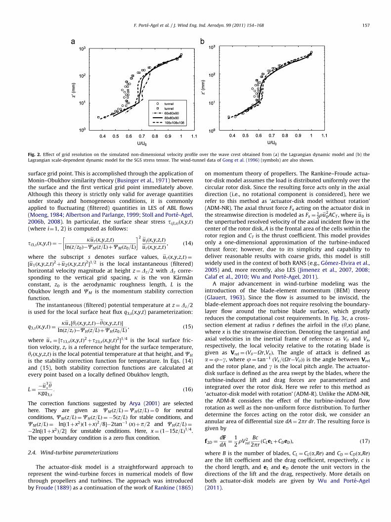
Fig. 2. Effect of grid resolution on the simulated non-dimensional velocity profile over the wave crest obtained from (a) the Lagrangian dynamic model and (b) the

Lagrangian scale-dependent dynamic model for the SGS stress tensor. The wind-tunnel data of Gong et al. (1996) (symbols) are also shown.

F. Porte-Agel et al. / J. Wind Eng. Ind. Aerodyn. 99 (2011) 154–168 157

surface grid point. This is accomplished through the application ofMonin–Obukhov similarity theory (Businger et al., 1971) betweenthe surface and the first vertical grid point immediately above.Although this theory is strictly only valid for average quantitiesunder steady and homogeneous conditions, it is commonlyapplied to fluctuating (filtered) quantities in LES of ABL flows(Moeng, 1984; Albertson and Parlange, 1999; Stoll and Porte-Agel,2006b, 2008). In particular, the surface shear stress tðb,sÞðx,y,tÞ(where i¼1, 2) is computed as follows:

ti3,sðx,y,tÞ ¼�keurðx,y,z,tÞ

lnðz=z0Þ�CMðz=LÞþCMðz0=LÞ

� �2 euiðx,y,z,tÞeurðx,y,z,tÞ, ð14Þ

where the subscript s denotes surface values, eurðx,y,z,tÞ ¼½eu1ðx,y,z,tÞ2þeu2ðx,y,z,tÞ2�1=2 is the local instantaneous (filtered)horizontal velocity magnitude at height z¼Dz=2 with Dz corre-sponding to the vertical grid spacing, k is the von Karmanconstant, z0 is the aerodynamic roughness length, L is theObukhov length and CM is the momentum stability correctionfunction.

The instantaneous (filtered) potential temperature at z¼Dz=2is used for the local surface heat flux q3,s(x,y,t) parameterization:

q3,sðx,y,tÞ ¼keu�½yrðx,y,z,tÞ�eyðx,y,z,tÞ�

lnðz=zrÞ�CHðz=LÞþCHðz0=LÞ, ð15Þ

where eu� ¼ ½t13,sðx,y,tÞ2þt23,sðx,y,tÞ2�1=4 is the local surface fric-tion velocity, zr is a reference height for the surface temperature,yrðx,y,z,tÞ is the local potential temperature at that height, and CH

is the stability correction function for temperature. In Eqs. (14)and (15), both stability correction functions are calculated atevery point based on a locally defined Obukhov length,

L¼�eu3�ey

kgq3,s: ð16Þ

The correction functions suggested by Arya (2001) are selectedhere. They are given as CMðz=LÞ ¼CHðz=LÞ ¼ 0 for neutralconditions, CMðz=LÞ ¼CHðz=LÞ ¼�5ðz=LÞ for stable conditions, andCMðz=LÞ ¼ ln½ð1þx2Þð1þxÞ2=8��2tan�1 ðxÞþp=2 and CHðz=LÞ ¼

�2ln½ð1þx2Þ=2� for unstable conditions. Here, x¼ ð1�15z=LÞ1=4.The upper boundary condition is a zero flux condition.

2.4. Wind-turbine parameterizations

The actuator-disk model is a straightforward approach torepresent the wind-turbine forces in numerical models of flowthrough propellers and turbines. The approach was introducedby Froude (1889) as a continuation of the work of Rankine (1865)

on momentum theory of propellers. The Rankine–Froude actua-tor-disk model assumes the load is distributed uniformly over thecircular rotor disk. Since the resulting force acts only in the axialdirection (i.e., no rotational component is considered), here werefer to this method as ‘actuator-disk model without rotation’(ADM-NR). The axial thrust force Fx acting on the actuator disk inthe streamwise direction is modeled as Fx ¼

12reu2

0ACT , where eu0 isthe unperturbed resolved velocity of the axial incident flow in thecenter of the rotor disk, A is the frontal area of the cells within therotor region and CT is the thrust coefficient. This model providesonly a one-dimensional approximation of the turbine-inducedthrust force; however, due to its simplicity and capability todeliver reasonable results with coarse grids, this model is stillwidely used in the context of both RANS (e.g., Gomez-Elvira et al.,2005) and, more recently, also LES (Jimenez et al., 2007, 2008;Calaf et al., 2010; Wu and Porte-Agel, 2011).

A major advancement in wind-turbine modeling was theintroduction of the blade-element momentum (BEM) theory(Glauert, 1963). Since the flow is assumed to be inviscid, theblade-element approach does not require resolving the boundary-layer flow around the turbine blade surface, which greatlyreduces the computational cost requirements. In Fig. 3c, a cross-section element at radius r defines the airfoil in the ðy,xÞ plane,where x is the streamwise direction. Denoting the tangential andaxial velocities in the inertial frame of reference as Vy and Vx,respectively, the local velocity relative to the rotating blade isgiven as Vrel ¼ ðVy�Or,VxÞ. The angle of attack is defined asa¼j�g, where j¼ tan�1 ðVx=ðOr�VyÞÞ is the angle between Vrel

and the rotor plane, and g is the local pitch angle. The actuator-disk surface is defined as the area swept by the blades, where theturbine-induced lift and drag forces are parameterized andintegrated over the rotor disk. Here we refer to this method as‘actuator-disk model with rotation’ (ADM-R). Unlike the ADM-NR,the ADM-R considers the effect of the turbine-induced flowrotation as well as the non-uniform force distribution. To furtherdetermine the forces acting on the rotor disk, we consider anannular area of differential size dA¼ 2pr dr. The resulting force isgiven by

f2D ¼dF

dA¼

1

2rV2

rel

Bc

2prðCLeLþCDeDÞ, ð17Þ

where B is the number of blades, CL ¼ CLða,ReÞ and CD ¼ CDða,ReÞ

are the lift coefficient and the drag coefficient, respectively, c isthe chord length, and eL and eD denote the unit vectors in thedirections of the lift and the drag, respectively. More details onboth actuator-disk models are given by Wu and Porte-Agel(2011).

Fig. 3. Schematic of the blade-element momentum approach: (a) three-dimensional view of a wind turbine; (b) a discretized blade; and (c) cross-section airfoil element

showing velocities and force vectors.

F. Porte-Agel et al. / J. Wind Eng. Ind. Aerodyn. 99 (2011) 154–168158

In the generalized actuator-disk and related models, theturbine-induced forces (lift, drag and thrust) are parameterizedand integrated over the entire rotor disk, making it impossible tocapture helicoidal tip vortices (Vermeer et al., 2003). To overcomethis limitation, a three-dimensional actuator-line model (ALM)was developed by Sørensen and Shen (2002). The ALM uses BEMtheory to calculate the turbine-induced lift and drag forces anddistributes them along lines representing the blades. As a result, ithas the ability to capture important features of turbine wakes,such as tip vortices and coherent periodic helicoidal vortices inthe near-wake region (Sørensen and Shen, 2002; Troldborg et al.,2007; Ivanell et al., 2009). The resulting turbine-induced force iscalculated as

f1D ¼dF

dr¼

1

2rV2

relcðCLeLþCDeDÞ: ð18Þ

In the above-mentioned wind-turbine models, the blade-induced forces are distributed smoothly to avoid singular beha-vior and numerical instability. In practice, these forces aredistributed in a three-dimensional Gaussian manner by takingthe convolution of the computed local load, f, and a regularizationkernel Ze as shown below:

fe ¼1

DvðF� ZeÞ, Ze ¼

1

e3p3=2exp �

rp2

e2

� �, ð19Þ

where Dv is the volume of a grid cell, rp is the distance betweengrid points and points representing the actuator disk or theactuator line, and e is a parameter that adjusts the distributionof the regularized load.

The main advantage of representing the blades by airfoil datais that much fewer grid points are needed to capture the influenceof the blades compared to what would be needed for simulatingthe actual geometry of the blades. Therefore, the ADM-R andALM are well suited for studies of turbine wakes (from stand-alone or multiple turbines) that require simulating largedomains to capture all the important scales of both ABL andturbine wake flows, while keeping the computing cost at areasonable level.

The effects of the nacelle and the turbine tower on theturbulent flow are modeled as drag forces fnacelle and ftower,respectively, by using a formulation similar to the ADM-NR anda drag coefficient based on the specific geometry. More details onthis approach are given by Wu and Porte-Agel (2011). As a result,the total immersed force fi associated with wind-turbine effects in

the filtered momentum equation (Eq. (2)) is given by

fi ¼ ðfeþfnacelle

þftowerÞ � ei, ð20Þ

where ei is the unit vector in the i-th direction.

3. Validation of the LES framework

In this section, the above-described LES framework is validatedusing high-resolution velocity measurements collected in thewake of a three-blade miniature wind turbine placed in a wind-tunnel boundary layer flow. The experiment is describedby Chamorro and Porte-Agel (2010). A modified version of theLES code described by Albertson and Parlange (1999), Porte-Agelet al. (2000), Porte-Agel (2004) and Stoll and Porte-Agel (2006a) isused. In this study, the three wind-turbine models (ADM-NR,ADM-R and ALM) for the turbine-induced forces are implementedin the LES code and used to simulate the wind-tunnel case, i.e., aneutral boundary-layer flow through a stand-alone wind turbineover a flat homogeneous surface. The main features of the codeand a brief description of the case study are given below. Moredetails on the numerical setup are provided by Wu and Porte-Agel(2011).

3.1. Numerical setup

As shown in Fig. 4, the computational domain has a heightLz¼0.460 m, corresponding to the top of the boundary layer H.The horizontal computational domain spans a distanceLx¼4.320 m in the streamwise direction and Ly ¼ 0.720 m inthe spanwise direction. The domain is divided uniformly intoNx�Ny�Nz¼192�32�42 grid points. The grid arrangement isstaggered in the vertical direction with the first level of computa-tion for the vertical velocity ew at a height of Dz ¼ Lz=ðNz�1Þ andthe first level for eu, ev and ep� at Dz=2. The LES code uses a hybridpseudospectral finite-difference method, i.e., spatial derivativesare computed using pseudospectral methods in the horizontaldirections and finite differences in the vertical direction. Timeadvancement is discretized using an explicit second-orderAdams–Bashforth scheme. Lateral boundary conditions are peri-odic, which is a seamless choice for pseudospectral methods. Thebottom and top boundary conditions are described in Section 2.3.The flow is driven by a constant streamwise pressure gradient.The friction velocity and aerodynamic surface roughness are0.102 m/s and 0.03 mm, respectively.

F. Porte-Agel et al. / J. Wind Eng. Ind. Aerodyn. 99 (2011) 154–168 159

The wind turbine used by Chamorro and Porte-Agel (2010) inthe wind-tunnel experiment consists of a three-blade GWS/EP-6030�3 rotor attached to a small DC generator motor. The rotordiameter d and the hub height Hhub of the turbine are 0.150 m and0.125 m, respectively. In the simulations, the blade section isviewed as a flat plate, whose lift and drag coefficients aredetermined based on a previous experimental study by Sunadaet al. (1997). The radial variation of the chord length and pitchangle of the turbine blade is given by Wu and Porte-Agel (2011).The wind turbine is placed in the middle of the computationaldomain at a distance of six rotor diameters from the upstreamboundary. To avoid that the flow upwind of the turbine isinfluenced by the turbine-induced wake flow (due to the periodicboundary conditions), we adopt a buffer zone (Fig. 4) to adjust theflow from the very-far-wake downwind condition to that of anundisturbed boundary layer inflow condition. This inflow condi-tion is obtained from a separate simulation of the boundary-layer

0.36 (m) (~2.4d) 0.36 (m) (~2.4d)

Hhub = 0.125 (m)

R = 0.075 (m)L z=

0.46

(m)

Ly = 0.72 (m)

Buf

fer

zone

L z =

0.4

6 (m

)

2d

Fig. 4. Schematic of the simulation domain.

Fig. 5. Contours of the time-averaged streamwise velocity u (m/s) in the middle vertica

(c) ADM-R and (d) ALM.

flow corresponding to the upwind of the wind turbine in thewind-tunnel experiment of Chamorro and Porte-Agel (2010).

3.2. Comparison with wind-tunnel measurements

Each of the simulations performed with the three wind turbinemodels (ADM-NR, ADM-R and ALM) was run for a total duration offour physical minutes, with converged turbulence statistics averagedover the last two minutes. The spatial distribution of two keyturbulence statistics is used to characterize wind-turbine wakes:the time-averaged streamwise velocity u and the streamwise turbu-lence intensity su=uhub. The over-bar represents a temporal average.The experimental data were collected at x/d ¼ �1, 1, 2, y, 9, 10, 12,y, 18, 20 in the middle of the domain as well as y/d ¼ �0.7, �0.6,y, 0,6, 0.7 in a cross-section downwind of the turbine at x/d ¼ 5.Fig. 5 shows contours of the time-averaged streamwise velocity

Vx

R = 0.075 (m)

Hhub = 0.125 (m)

4d 22.8d

Lx = 28.8 d = 4.32 (m)

Front view (left) and side view (right).

l plane perpendicular to the turbine: (a) wind-tunnel measurements, (b) ADM-NR,

F. Porte-Agel et al. / J. Wind Eng. Ind. Aerodyn. 99 (2011) 154–168160

obtained from the wind-tunnel experiment and simulations with theADM-NR, ADM-R and ALM on a vertical plane perpendicular to theturbine. Furthermore, to facilitate the quantitative comparison ofthe results, Fig. 6 shows vertical profiles of the measured andsimulated time-averaged streamwise velocity at selected downwindlocations (x/d¼2, 3, 5, 7, 10, 14, 20), together with the incoming flowvelocity profile. There is a clear evidence of the effect of the turbineextracting momentum from the incoming flow and producing a wake(region of reduced velocity) immediately downwind. As expected, thevelocity deficit (reduction with respect to the incoming flow) islargest near the turbine and it becomes smaller as the wake expandsand entrains surrounding air. Nonetheless, the effect of the wake isstill noticeable even in the far wake, at distances as large as x/d¼20.Further, due to the non-uniform (logarithmic) mean velocity profile ofthe incoming boundary-layer flow, we find a non-axisymmetricdistribution of the mean velocity profile and, consequently, of themean shear in the turbine wake. In particular, as also reportedby Chamorro and Porte-Agel (2009, 2010), the strongest shear(and the associated turbulence kinetic energy production) is foundat the level of the top tip. This result contrasts with the axisymmetryof the turbulence statistics reported by previous studies in the case ofwakes of turbines placed in free-stream flows (Crespo andHernandez, 1996; Medici and Alfredsson, 2006; Troldborg et al.,2007), and demonstrates the substantial influence of the incomingflow on the structure and dynamics of wind-turbine wakes.

x/d = –1 x/d = –2

z/d

Wind spe1.2 1.6 2 2.4 2.8 1.2 1.6 2 2.4 2.8

0

1

2

z/d

Wind speed1.2 1.6 2 2.4 2.8 1.2 1.6 2 2.4 2.8

0

1

2x/d = –7 x/d = –10

Fig. 6. Comparison of vertical profiles of the time-averaged streamwise velocity u (m/

ALM (dotted line).

1.6

1.7

1.8

1.92

2.1

2.2

2.3

2.4

y/d

z/d

–0.6 –0.3 0 0.3 0.6

0.3

0.6

0.9

1.2

1.5

1.7

1.81.9

22.12.2

y/d–0.6 –0.3 0 0.3 0.6

0.3

0.6

0.9

1.2

1.5

Fig. 7. Contours of the time-averaged streamwise velocity u (m/s) at the lateral cross

ADM-NR, ADM-R and ALM (from left to right). The dashed line represents the turbine

As shown in Figs. 5 and 6, the LES results obtained from theADM-R and ALM show that the mean velocity profiles are in goodagreement with the measurements everywhere in the turbinewake (near wake as well as far wake). The ADM-NR is able tocapture the velocity distribution in the far-wake region ðx=d45Þ,but it clearly overpredicts the velocity in the center of the wake inthe near-wake region ðx=do5Þ. This failure of the ADM-NR toreproduce the velocity magnitude in the near-wake region can beattributed to the limitations of two important assumptions madein the ADM-NR (but not in the other wind-turbine models):(a) the effect of turbine-induced rotation is ignored, and (b) theforce is uniformly distributed over the rotor disk, thus ignoringthe radial variation of the force. These two assumptions are incontrast with simulation results of the non-uniform force dis-tribution reported by Sørensen and Shen (2002). It is important tonote that, as discussed by Wu and Porte-Agel (2011), accountingfor the non-uniform distribution of the thrust force is responsiblefor most of the improvement observed in the ADM-R with respectto the ADM-NR.

Contours of the average velocity at the lateral cross-sectionand downwind location x/d ¼ 5 are shown in Fig. 7. The resultsshow the non-axisymmetry (with respect to the turbine axis) ofthe velocity distribution due to the non-uniformity of the incom-ing flow and the presence of the surface. Simulation results of themean resolved velocity obtained from both the ALM and the

x/d = –3 x/d = –5

ed (ms–1)1.2 1.6 2 2.4 2.8 1.2 1.6 2 2.4 2.8

(ms–1)1.2 1.6 2 2.4 2.8 1.2 1.6 2 2.4 2.8

x/d = –14 x/d = –20

s): wind-tunnel measurements (3), ADM-NR (dashed line), ADM-R (solid line) and

1.61.7

1.81.9 22.12.2

y/d–0.6 –0.3 0 0.3 0.6

0.3

0.6

0.9

1.2

1.5

1.61.7

1.81.9 22.12.2

y/d–0.6 –0.3 0 0.3 0.6

0.3

0.6

0.9

1.2

1.5

-section and downstream x/d¼5 obtained from the wind-tunnel measurements,

region.

F. Porte-Agel et al. / J. Wind Eng. Ind. Aerodyn. 99 (2011) 154–168 161

ADM-R are in reasonable agreement with the measurements,with only a small difference in the magnitude of the velocity forboth models. However, the ADM-NR yields a poor prediction ofthe mean velocity distribution in comparison with the wind-tunnel experimental data.

Fig. 8. Contours of the streamwise turbulence intensity su=uhub in the middle vertical

(c) ADM-R and (d) ALM.

x/d = –1 x/d = 2

z/d

Turbulence

0.04 0.08 0.12 0.16 0.04 0.08 0.12 0.160

1

2

z/d

Turbulence

0.04 0.08 0.12 0.16 0.04 0.08 0.12 0.160

1

2

x/d = 7 x/d = 10

Fig. 9. Comparison of vertical profiles of the streamwise turbulence intensity su=uhub: w

(dotted line).

Fig. 8 shows contours of the streamwise turbulence intensitysu=uhub obtained from the wind-tunnel measurements and simu-lations (resolved part) using LES with the ADM-NR, ADM-R andALM on a vertical plane perpendicular to the turbine. Verticalprofiles of measured and simulated turbulence intensities at

plane perpendicular to the turbine: (a) wind-tunnel measurements, (b) ADM-NR,

x/d = 3 x/d = 5

intensity

0.04 0.08 0.12 0.16 0.04 0.08 0.12 0.16

intensity

0.04 0.08 0.12 0.16 0.04 0.08 0.12 0.16

x/d = 14 x/d = 20

ind-tunnel measurements (3), ADM-NR (dashed line), ADM-R (solid line) and ALM

0.07

0.08

0.0

0.09

0.1

0.1

0.110.12

12 0.13

y/d

z/d

–0.6 –0.3 0 0.3 0.6

0.3

0.6

0.9

1.2

1.5 0.07

0.08

0.08

0.09

0.09

0.1

0.1

0.1

0.11

0.11

y/d

–0.6 –0.3 0 0.3 0.6

0.3

0.6

0.9

1.2

1.5 0.07 0.08

09

0.09

0.09

0.1

0.1

0.11

0.11

0.12

0.13

y/d

–0.6 –0.3 0 0.3 0.6

0.3

0.6

0.9

1.2

1.50.07 0.08

0.09

0.09

0.09

0.1

0.1

0.11

0.11

0.12

0.13

y/d

–0.6 –0.3 0 0.3 0.6

0.3

0.6

0.9

1.2

1.5

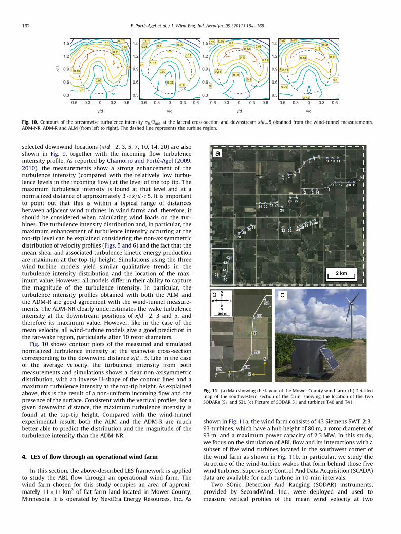
Fig. 10. Contours of the streamwise turbulence intensity su=uhub at the lateral cross-section and downstream x/d¼5 obtained from the wind-tunnel measurements,

ADM-NR, ADM-R and ALM (from left to right). The dashed line represents the turbine region.

Fig. 11. (a) Map showing the layout of the Mower County wind farm. (b) Detailed

map of the southwestern section of the farm, showing the location of the two

SODARs (S1 and S2). (c) Picture of SODAR S1 and turbines T40 and T41.

F. Porte-Agel et al. / J. Wind Eng. Ind. Aerodyn. 99 (2011) 154–168162

selected downwind locations (x/d¼2, 3, 5, 7, 10, 14, 20) are alsoshown in Fig. 9, together with the incoming flow turbulenceintensity profile. As reported by Chamorro and Porte-Agel (2009,2010), the measurements show a strong enhancement of theturbulence intensity (compared with the relatively low turbu-lence levels in the incoming flow) at the level of the top tip. Themaximum turbulence intensity is found at that level and at anormalized distance of approximately 3ox=do5. It is importantto point out that this is within a typical range of distancesbetween adjacent wind turbines in wind farms and, therefore, itshould be considered when calculating wind loads on the tur-bines. The turbulence intensity distribution and, in particular, themaximum enhancement of turbulence intensity occurring at thetop-tip level can be explained considering the non-axisymmetricdistribution of velocity profiles (Figs. 5 and 6) and the fact that themean shear and associated turbulence kinetic energy productionare maximum at the top-tip height. Simulations using the threewind-turbine models yield similar qualitative trends in theturbulence intensity distribution and the location of the max-imum value. However, all models differ in their ability to capturethe magnitude of the turbulence intensity. In particular, theturbulence intensity profiles obtained with both the ALM andthe ADM-R are good agreement with the wind-tunnel measure-ments. The ADM-NR clearly underestimates the wake turbulenceintensity at the downstream positions of x/d¼2, 3 and 5, andtherefore its maximum value. However, like in the case of themean velocity, all wind-turbine models give a good prediction inthe far-wake region, particularly after 10 rotor diameters.

Fig. 10 shows contour plots of the measured and simulatednormalized turbulence intensity at the spanwise cross-sectioncorresponding to the downwind distance x/d¼5. Like in the caseof the average velocity, the turbulence intensity from bothmeasurements and simulations shows a clear non-axisymmetricdistribution, with an inverse U-shape of the contour lines and amaximum turbulence intensity at the top-tip height. As explainedabove, this is the result of a non-uniform incoming flow and thepresence of the surface. Consistent with the vertical profiles, for agiven downwind distance, the maximum turbulence intensity isfound at the top-tip height. Compared with the wind-tunnelexperimental result, both the ALM and the ADM-R are muchbetter able to predict the distribution and the magnitude of theturbulence intensity than the ADM-NR.

4. LES of flow through an operational wind farm

In this section, the above-described LES framework is appliedto study the ABL flow through an operational wind farm. Thewind farm chosen for this study occupies an area of approxi-mately 11�11 km2 of flat farm land located in Mower County,Minnesota. It is operated by NextEra Energy Resources, Inc. As

shown in Fig. 11a, the wind farm consists of 43 Siemens SWT-2.3-93 turbines, which have a hub height of 80 m, a rotor diameter of93 m, and a maximum power capacity of 2.3 MW. In this study,we focus on the simulation of ABL flow and its interactions with asubset of five wind turbines located in the southwest corner ofthe wind farm as shown in Fig. 11b. In particular, we study thestructure of the wind-turbine wakes that form behind those fivewind turbines. Supervisory Control And Data Acquisition (SCADA)data are available for each turbine in 10-min intervals.

Two SOnic Detection And Ranging (SODAR) instruments,provided by SecondWind, Inc., were deployed and used tomeasure vertical profiles of the mean wind velocity at two

F. Porte-Agel et al. / J. Wind Eng. Ind. Aerodyn. 99 (2011) 154–168 163

locations in the wind farm (labeled S1 and S2 in Fig. 11b). The firstSODAR (S1) was placed midway between turbines T39 and T40with the intention of measuring the background atmosphericwind profile during periods when the wind was blowing from thesouth (the prevailing wind direction). Fig. 11c shows a picture ofthis SODAR and turbines T40 and T41. The second SODAR (S2)was placed between turbines T41 and T42 (specifically at adistance of four rotor diameters downwind of T41) with theintention of measuring the wake of T41 during southerly windconditions. The SODARs measure the vertical wind profile usingthree beams, each 101 off the vertical, and separated horizontallyby 1201. The half power beam width is approximately 111. Pulsesfrom each of these three beams are sent out at approximately 10 sintervals, and the return signals are averaged over a 10-minperiod to calculate the vertical wind profile. The measured windprofiles include all three components of velocity at heights of 40,50, 60, 80, 100, 120, 140, 160, 180, and 200 m above groundlevel. Table 1 shows the coordinates of the two SODARs as well asthe five wind turbines with respect to the XY reference systemshown in Fig. 11b.

4.1. Case description

The period of November 22, 2009, between 2100 and 2200UTC, was chosen for our case study because of the relativelysimple and quasi-stationary atmospheric boundary layer condi-tions. During that period, atmospheric stability was near-neutral,atmospheric conditions were favorable for good SODAR echoes,and the wind blew from the south with quasi-stationary magni-tude and direction. This study focuses on wind-turbine wakes inhigh-Reynolds-number neutrally stratified ABL flow, and there-fore viscous, molecular, Coriolis and buoyancy effects areneglected in the simulations. Based on a semi-logarithmic fit ofthe velocity profile measured during the study period by theSODAR at the S1 location (not affected by turbine wakes), one cancalculate a frictional velocity of un¼0.63 m/s and a surfaceroughness of z0¼0.3 m. The size of the simulation domain is

Table 1Positions of wind turbines and SODARs associated with the XY coordinate system

shown in Fig. 11b.

T39 T40 T41 T42 T43 S1 S2

X (m) 0 93 385 1062 1425 44 780

Y (m) 917 412 232 200 0 665 240

4 6 8 10 120

50

100

150

200

250

u (m/s)

z (m

)

S1 (LES)S2 (LES–ADM–NR)S2 (LES–ADM–R)S2 (LES–ALM)S1 (SODAR)S2 (SODAR)

Fig. 12. Comparison of vertical profiles of time-averaged streamwise velocity u (m/s) (a

using LES with different wind-turbine models. Also plotted are the mean wind velocit

Lx¼2400 m, Ly¼1200 m and Lz¼700 m in the streamwise, span-wise and vertical directions, respectively. The domain is divideduniformly into Nx�Ny�Nz¼192�192�112 grid points, with aspatial resolution of Dx ¼ 12:5 m and Dy ¼Dz ¼ 6:25 m. As aresult, each turbine rotor disk is covered by 15 points in bothspanwise and vertical directions. A buffer zone technique is alsoimplemented at a distance of four rotor diameters upwind of thewind farm to adjust the flow from the very-far-wake downwindcondition to that of an undisturbed boundary layer inflow condi-tion. The inflow condition is obtained from a separate simulationof the boundary-layer flow corresponding to the upwind of thewind farm in the field measurements.

In the LESs of the wind farm case considered here, the wind-turbine-induced forces are modeled using the three models(ADM-NR, ADM-R and ALM) presented in Section 2. The SGSmomentum flux is parameterized using the Lagrangian scale-dependent dynamic model. Some of the parameters required forthe wind-turbine models, such as turbine angular velocity, tur-bine power output, and blade pitch angle, are obtained from theSCADA data set. During the one-hour period under consideration,the mean wind speed at the hub height was approximately 9 m/s,which leads to the Siemens SWT-2.3-93 turbines operating with amean angular velocity of 15 rpm and producing a mean power of1.4 MW. The geometry of the B45 blade that is part of the SiemensSWT-2.3-93 turbines is given by Leloudas (2006). Laursen et al.(2007) used computational fluid dynamics to characterize theangle of attack and the lift and drag coefficients along the B45blade. In the ADM-NR, a constant and uniform thrust coefficient(CT) is used in the simulation. To estimate this thrust coefficientbased on the mean turbine power available from the SCADA data,we first compute the power coefficient (ratio of turbine power topower available in the wind) Cp¼0.47. Then, assuming themechanical efficiency of the turbine to be Zmech ¼ 1, and usingthe following relationships derived from one-dimensionalmomentum theory (Manwell et al., 2002),

Cp ¼ 4að1�aÞ2 ð21Þ

and

CT ¼ 4að1�aÞ, ð22Þ

where a is the overall induction factor, we obtain a¼0.17 and anoverall thrust coefficient of CT¼0.57, which is then used in theADM-NR. Due to the resolution limitations of LES, effects asso-ciated with the aeroelastic behavior of the turbines are notconsidered here. All simulations have been run for 1.5 h of real

0.09 0.12 0.15 0.18 0.210

50

100

150

200

250

Turbulence intensity

z (m

)

S1 (LES)S2 (LES–ADM–NR)S2 (LES–ADM–R)S2 (LES–ALM)

) and streamwise turbulence intensity su=uhub (b) simulated at locations S1 and S2

y profiles measured with the two SODARs.

F. Porte-Agel et al. / J. Wind Eng. Ind. Aerodyn. 99 (2011) 154–168164

time to guarantee quasi-steady flow conditions. Results arepresented here for the last half-hour of the simulations.

4.2. Simulation results

Fig. 12a shows the time-averaged streamwise velocity profilesat the S1 and S2 locations (see Fig. 11b) obtained from bothSODAR measurements and numerical simulations. Overall, thevelocity profiles obtained from the ADM-R and the ALM are ingood agreement with the SODAR measurements. The ADM-NRslightly overestimates the magnitude of the velocity in the near-wake region. This slight underestimation of the velocity deficit bythe ADM-NR is consistent with the simulation results on thewind-tunnel case (Section 3). As discussed in Section 3, this canbe attributed to limitations of the two key assumptions made inthe ADM-NR: ignoring turbine-induced rotation effects, andassuming uniform thrust distribution over the rotor disk.

Fig. 12b shows vertical profiles of the streamwise turbulenceintensity obtained from simulations with the three wind-turbinemodels at the S1 and S2 locations. It is obvious that the threemodels yield an enhancement of the turbulence intensity at thetop-tip level (compared with the relatively lower turbulenceintensity in the incoming flow). This turbulence intensityenhancement has also been reported in wind-tunnel and LESstudies, as described in Section 3. The magnitude of the maximumturbulence intensity obtained from both the ADM-R and the ALMis larger than the one from the ADM-NR, which is also consistentwith the simulation results presented in Section 3 for the wind-tunnel case.

Two-dimensional contour plots of the simulated time-aver-aged streamwise velocity obtained with the three wind-turbinemodels on a horizontal plane at hub height, as well as on avertical plane perpendicular to the middle of the rotor of turbineT41, are shown in Figs. 13 and 14, respectively. As expected,turbine wakes (regions of reduced mean velocity) are clearly

Fig. 13. Two-dimensional contour plots of the simulated time-averaged streamwise v

(c) ALM.

visible behind each wind turbine. From Fig. 13, the effect of thewake induced by turbine T39 is still noticeable in the far-wakeregion at distances as far as 1700 m (approximately 18 rotordiameters downwind), which is consistent with the wind-tunnelobservations. The largest velocity reduction, relative to theincoming boundary-layer flow, is observed in the wake of turbineT42. This is due to the fact that, for that wind direction, turbineT42 is located in the wake of turbine T41. Also consistent with thewind-tunnel case simulations presented in Section 3, the ADM-NRoverestimates the magnitude of the near-wake velocity (thusunderestimating the velocity deficit) compared with both ADM-Rand ALM. In the case of the Siemens SWT-2.3-93 wind turbine,some differences are also observed between the near-wake meanvelocity simulated with the ADM-R and ALM.

In order to understand the effect of the simulated wakes onturbine power reduction, the available wind power at one rotordiameter upwind of each turbine has been computed usingP¼ 0:5rAU

3

rotor , where U rotor is the average velocity integratedover the whole rotor area (A). It should be noted that the wakeinduced by turbine T41 results in a substantial power reductionðrP ð1�PT42=PT41Þ � 100%Þ on the flow upwind of turbine T42.The rp values obtained from the simulations with ALM and ADM-Rare, respectively, 47% and 50%, which are very close to the actualwind turbine power reduction of 48% based on the SCADA data.The ADM-NR yields a lower power reduction value of 37%, due tothe overprediction of the velocity magnitude in the wake inducedby turbine T41.

Two-dimensional contour plots of the time-averaged verticalvelocity component, simulated using LES with the three wind-turbine models, are shown in Fig. 15 for a horizontal plane at hubheight. The positive and negative vertical velocities obtained withthe ADM-R and ALM on both sides of the wakes highlight theability of those models to induce wake rotation. As expected, thewakes rotate in counter-clockwise direction (for an observerlocated upwind of the turbine), which is opposite to the clockwiserotation of the turbine blades. It should be noted that the vertical

elocity u (m/s) on a horizontal plane at hub height: (a) ADM-NR, (b) ADM-R and

Fig. 14. Two-dimensional contour plots of the simulated time-averaged streamwise velocity u (m/s) on a vertical plane perpendicular to the rotor (and through the

middle) of turbine T41: (a) ADM-NR, (b) ADM-R and (c) ALM.

Fig. 15. Two-dimensional contour plots of the simulated time-averaged vertical velocity w (m/s) on a horizontal plane at hub height: (a) ADM-NR, (b) ADM-R and (c) ALM.

F. Porte-Agel et al. / J. Wind Eng. Ind. Aerodyn. 99 (2011) 154–168 165

velocity distribution in the wakes is non-symmetric, with thepositive velocity region extending further downwind comparedwith the negative velocity. The non-axisymmetry of the wake isconsequence of the interactions of the rotating wake flow withboth the land surface and the non-uniform (logarithmic) incom-ing boundary layer flow. Note that the ADM-NR is unable toaccount for wake rotation because it only considers the thrust

force and ignores any forces parallel to the rotor plane, which areresponsible for the rotation of the wake flow.

Two-dimensional contours of the simulated streamwise tur-bulence intensity obtained with the three wind-turbine modelson a vertical plane perpendicular to the middle of the rotor ofturbine T41 are shown in Fig. 16. From that figure, it is clear thatthe three turbine models lead to an enhancement of the

Fig. 16. Two-dimensional contour plots of the simulated streamwise turbulence intensity su=uhub on a vertical plane perpendicular to the rotor (and through the middle)

of turbine T41: (a) ADM-NR, (b) ADM-R and (c) ALM.

F. Porte-Agel et al. / J. Wind Eng. Ind. Aerodyn. 99 (2011) 154–168166

turbulence intensity at the top-tip height. The maximum simu-lated turbulence intensity at that height is higher (by about 20%)than the one observed for the wind-tunnel case. However, owingto the larger turbulence levels in the incoming flow for the fieldcase, the increase in the turbulence intensity (with respect to theincoming flow levels) is similar for both cases. Furthermore, themaximum turbulence intensity at that height is found at anormalized distance of approximately 1ox=do3 downwind ofturbines T41 and T42. It should be noted that this distance fromthe wind turbines to the peak of turbulence intensity is shorterthan the one found for the wind-tunnel case (approximately3ox=do5, as shown in Fig. 8). This result is consistent withprevious observations that the extent of the near-wake regionmeasured in wind-tunnel experiments is typically longer thanthat measured in the field (Helmis et al., 1995). It also highlightssome of the challenges associated with the design of wind-tunnelexperiments to study the structure and dynamics of wind-turbinewakes, especially in the near-wake region, where the details ofthe blades and the incoming flow characteristics (e.g., turbulenceintensity) are likely to play an important role.

5. Summary

This paper presents recent efforts to develop and validate alarge-eddy simulation framework for wind energy applications.The tuning-free Lagrangian scale-dependent dynamic models areused to parameterize the SGS stress tensor and the SGS heat flux.Three types of models are used to parameterize the turbine-induced forces: a standard actuator-disk model without rotation(ADM-NR) that computes an overall thrust force and distributes ituniformly over the rotor disk area; an actuator-disk model withrotation (ADM-R) that computes the local lift and drag forces(based on blade-element momentum theory) and distributes

them on the rotor disk area; and an actuator-line model (ALM)that distributes those forces along lines that follow the position ofthe blades.

The proposed LES framework is validated against high-resolu-tion velocity measurements collected in the wake of a miniaturewind turbine placed in a wind-tunnel boundary layer flow. Ingeneral, the characteristics of the simulated turbine wakes (aver-age velocity and turbulence intensity distributions) are in goodagreement with the measurements. The comparison with thewind-tunnel measurements shows that the turbulence statisticsobtained with the LES and the ADM-NR have some differenceswith respect to the measurements in the near-wake region. Inparticular, the model overestimates the average velocity in thecenter of the wake, while underestimating the turbulence inten-sity at the top-tip level, where turbulence levels are highest dueto the presence of a strong shear layer. The ADM-R and ALM yieldmore accurate predictions of the different turbulence statistics inthe near-wake region. This highlights the importance of using awind-turbine model that induces wake rotation and allows fornon-uniform distribution of the turbine-induced forces. In the farwake, all three models produce reasonable results.

The proposed LES framework is also used to simulate ABL flowthrough an operational wind farm, where SODAR measurementsare available at two locations. Again, the ADM-R and the ALM arecapable of delivering accurate mean velocity profiles in the wake,with ADM-NR slightly underestimating the velocity deficit in thenear wake. The characteristics (velocity deficit and turbulenceintensity) of the simulated wakes behind the field-scale SiemensSWT-2.3-93 turbines show similar qualitative behavior comparedwith the stand-alone turbine wake measured in the wind tunnel.However, some quantitative differences have been found; thepeak of the turbulence intensity is larger (by about 20%) and itappears at a relatively shorter downwind distance from theturbine, compared with the wind-tunnel case. These differences

F. Porte-Agel et al. / J. Wind Eng. Ind. Aerodyn. 99 (2011) 154–168 167

are consistent with observations from previous wind-tunnel andfield studies of wind-turbine wakes (Vermeer et al., 2003), andthey can be attributed to differences in the turbines and theincoming flow characteristics (e.g., turbulence intensity) betweenthe wind tunnel and the field. Regarding turbine power predic-tion, simulations with both ADM-R and ALM are able to predictreductions in power associated with turbine wakes. Consistentwith the underestimation of the velocity deficit, the ADM-NR isfound to underestimate the power reduction in turbines operat-ing in wakes of other turbines.

The research presented here constitutes a step towards thedevelopment and the validation of a robust computational fluiddynamics framework for the study of atmospheric boundary layerflow and its interactions with wind turbines and wind farms. Thisframework can be used to optimize the design (turbine siting) ofwind energy projects (single turbines and wind farms) by increas-ing the efficiency, energy output and lifetime of wind turbines. Itcan also be used to study the effects of wind farms on localmeteorology. Future efforts will focus on further development,validation and application of this LES framework in a variety ofcases involving different atmospheric stability conditions (neu-tral, stable and unstable), land-surface characteristics (land coverand topography) and wind-farm layouts.

Acknowledgments

This research was supported by the Swiss National ScienceFoundation (Grant 200021_132122), the National Science Foun-dation (Grants EAR-0537856 and ATM-0854766), NASA (GrantNNG06GE256), customers of Xcel Energy through a Grant (RD3-42) from the Renewable Development Fund, and the University ofMinnesota Institute for Renewable Energy and the Environment.Computing resources were provided by the Minnesota Super-computing Institute. The SODARs were provided by SecondWind,Inc., and Barr Engineering Company assisted with theirdeployment.

References

AGARD, 1998. A selection of test cases for the validation of large-eddy simulationsof turbulent flows. AGARD Advisory Report 345.

Albertson, J.D., Parlange, M.B., 1999. Surface length scales and shear stress:implications for land–atmosphere interaction over complex terrain. WaterResour. Res. 35, 2121–2132.

Alinot, C., Masson, C., 2002. Aerodynamic simulations of wind turbines operatingin atmospheric boundary layer with various thermal stratifications. In: ASMEWind Energy Symposium AIAA, 2002-42.

Arya, S.P., 2001. Introduction to Micrometeorology, second ed. vol. 79. AcademicPress.

Baidya Roy, S., Pacala, S.W., Walko, R.L., 2004. Can large wind farms affect localmeteorology? J. Geophys. Res. 109, 1–6.

Bou-Zeid, E., Vercauteren, N., Meneveau, C., Parlange, M., 2008. Scale dependenceof subgrid-scale model coefficients: an a priori study. Phys. Fluids 20, 115106.

Businger, J.A., Wynagaard, J.C., Izumi, Y., Bradley, E.F., 1971. Flux–profile relation-ships in the atmospheric surface layer. J. Atmos. Sci. 28, 181–189.

Calaf, M., Meneveau, C., Meyers, J., 2010. Large eddy simulation study of fullydeveloped wind-turbine array boundary layers. Phys. Fluids 22, 015110.

Chamorro, L.P., Porte-Agel, F., 2009. A wind-tunnel investigation of wind-turbinewakes: boundary-layer turbulence effects. Boundary-Layer Meteorol. 132,129–149.

Chamorro, L.P., Porte-Agel, F., 2010. Effects of thermal stability and incomingboundary-layer flow characteristics on wind-turbine wakes: a wind-tunnelstudy. Boundary-Layer Meteorol., 515–533.

Crespo, A., Hernandez, J., 1996. Turbulence characteristics in wind-turbine wakes.J. Wind Eng. Ind. Aerodyn. 61, 71–85.

Froude, R.E., 1889. On the part played in propulsion by difference of fluid pressure.Trans. R. Inst. Naval Arch. 30, 390–423.

Germano, M., Piomelli, U., Cabot, W.H., 1991. A dynamic subgrid-scale eddyviscosity model. Phys. Fluids A 3, 1760–1765.

Glauert, H., 1963. Airplane propellers. In: Durand, W.F. (Ed.), Aerodynamic Theory.Dover, New York, pp. 169–360.

Gomez-Elvira, R., Crespo, A., Migoya, E., Manuel, F., Hernandez, J., 2005. Anisotropyof turbulence in wind turbine wakes. J. Wind. Eng. Ind. Aerodyn. 93,797–814.

Gong, W., Taylor, P.A., Darnbrack, A., 1996. Turbulent boundary-layer flow overfixed aerodynamically rough two-dimensional sinusoidal waves. J. Fluid Mech.312, 1–37.

Helmis, C.G., Papadopoulos, K.H., Asimakopoulos, D.N., Papageorgas, P.G., Soi-lemes, A.T., 1995. An experimental study of the near wake structure of a windturbine operating over complex terrain. Sol. Energy 54, 413–428.

Ivanell, S., Sørensen, J.N., Mikkelsen, R., Henningson, D., 2009. Analysis ofnumerically generated wake structures. Wind Energy 12, 63–80.

Jimenez, A., Crespo, A., Migoya, E., Garcia, J., 2007. Advances in large-eddysimulation of a wind turbine wake. J. Phys. Conf. Ser. 75, 012041.

Jimenez, A., Crespo, A., Migoya, E., Garcia, J., 2008. Large-eddy simulation ofspectral coherence in a wind turbine wake. Environ. Res. Lett. 3, 015004.

Kasmi, A.E., Masson, C., 2008. An extended k�e model for turbulent flow throughhorizontal-axis wind turbines. J. Wind. Eng. Ind. Aerodyn. 96, 103–122.

Kleissl, J., Meneveau, C., Parlange, M.B., 2003. On the magnitude and variability ofsubgrid-scale eddy-diffusion coefficients in the atmospheric surface layer.J. Atmos. Sci. 60, 2372–2388.

Kleissl, J., Parlange, M.B., Meneveau, C., 2004. Field experimental study of dynamicSmagorinsky models in the atmospheric surface layer. J. Atmos. Sci. 61,2296–2307.

Laursen, J., Enevoldsen, P., Hjort, S., 2007. 3D CFD rotor computations of a multimegawatt HAWT rotor. In: European Wind Energy Conference, Milan, Italy.

Leloudas, G., 2006. Optimization of wind turbines with respect to noise. MastersThesis Project, MEK, DTU.

Lilly, D.K., 1967. The representation of small-scale turbulence in numericalsimulation experiments. In: Proceedings of IBM Scientific Computing Sympo-sium on Environmental Sciences. IBM Data Processing Division, White Plains,NY, p. 195.

Lilly, D.K., 1992. A proposed modification of the Germano subgrid-scale closuremethod. Phys. Fluids 4, 633–635.

Manwell, J., McGowan, J., Rogers, A., 2002. Wind Energy Explained: Theory, Designand Application. Wiley, New York.

Mason, P.J., 1994. Large-eddy simulation: a critical review of the technique. Q. J. R.Meteorol. Soc. 120, 1–26.

Mason, P.J., Brown, A.R., 1999. On subgrid models and filter operations in largeeddy simulations. J. Atmos. Sci. 56, 2101–2114.

Mason, P.J., Derbyshire, S.H., 1990. Large-eddy simulation of the stably-stratifiedatmospheric boundary layer. Boundary-Layer Meteorol. 53, 117–162.

Mason, P.J., Thomson, D.J., 1992. Stochastic backscatter in large-eddy simulationsof boundary layers. J. Fluid Mech. 242, 51–78.

Medici, D., Alfredsson, P.H., 2006. Measurements on a wind turbine wake: 3Deffects and bluff body vortex shedding. Wind Energy 9, 219–236.

Meneveau, C., Lund, T.S., Cabot, W.H., 1996. A lagrangian dynamic subgrid-scalemodel of turbulence. J. Fluid Mech. 319, 353–385.

Moeng, C.H., 1984. A large-eddy-simulation model for the study of planetaryboundary-layer turbulence. J. Atmos. Sci. 41, 2052–2062.

Moin, P., Squires, K.D., Lee, S., 1991. A dynamic subgrid-scale model for compres-sible turbulence and scalar transport. Phys. Fluids 3, 2746–2757.

Petersen, E.L., Mortensen, N.G., Landberg, L., Højstrup, J., Frank, H.P., 1998.Wind power meteorology. Part 1: climate and turbulence. Wind Energy 1,25–45.

Pope, S.B., 2000. Turbulent Flows. Cambridge University Press, Cambridge.Porte-Agel, F., 2004. A scale-dependent dynamic model for scalar transport in

large-eddy simulations of the atmospheric boundary layer. Boundary-LayerMeteorol. 112, 81–105.

Porte-Agel, F., Meneveau, C., Parlange, M.B., 2000. A scale-dependent dynamicmodel for large-eddy simulation: application to a neutral atmospheric bound-ary layer. J. Fluid Mech. 415, 261–284.

Porte-Agel, F., Meneveau, C., Parlange, M.B., Eichinger, W.E., 2001. A priori fieldstudy of the subgrid-scale heat fluxes and dissipation in the atmosphericsurface layer. J. Atmos. Sci. 58, 2673–2698.

Rankine, W.J.M., 1865. On the mechanical principles of the action of propellers.Trans. R. Inst. Naval Arch. 6, 13–39.

Sagaut, P., 2006. Large Eddy Simulation for Incompressible Flows, third ed.Springer-Verlag, Berlin, Heidelberg.

Sezer-Uzol, N., Long, L.N., 2006. 3-D time-accurate CFD simulations of windturbine rotor flow fields. AIAA Paper 2006-0394.

Smagorinsky, J., 1963. General circulation experiments with the primitive equa-tions: I. The basic experiment. Mon. Weather Rev. 91, 99–164.

Sørensen, J.N., Shen, W.Z., 2002. Numerical modeling of wind turbine wakes.J. Fluids Eng. 124, 393–399.

Sørensen, N.N., Michelsen, J.A., Schreck, S., 2002. Navier-stokes predictions of theNREL phase VI rotor in the NASA Ames 80 ft� 120 ft wind tunnel. WindEnergy 5, 151–169.

Stoll, R., Porte-Agel, F., 2006a. Dynamic subgrid-scale models for momentumand scalar fluxes in large-eddy simulations of neutrally stratified atmos-pheric boundary layers over heterogeneous terrain. Water Resour. Res. 42,W01409.

Stoll, R., Porte-Agel, F., 2006b. Effect of roughness on surface boundary conditionsfor large-eddy simulation. Boundary-Layer Meteorol. 118, 169–187.

Stoll, R., Porte-Agel, F., 2008. Large-eddy simulation of the stable atmosphericboundary layer using dynamic models with different averaging schemes.Boundary-Layer Meteorol. 126, 1–28.

F. Porte-Agel et al. / J. Wind Eng. Ind. Aerodyn. 99 (2011) 154–168168

Sunada, S., Sakaguchi, A., Kawachi, K., 1997. Airfoil section characteristics at a lowReynolds number. J. Fluids Eng. 119, 129–135.

Tongchitpakdee, C., Benjanirat, S., Sankar, L.N., 2005. Numerical simulation of theaerodynamics of horizontal axis wind turbines under yawed flow conditions.J. Sol. Energy Eng. 127, 464–474.

Troldborg, N., Sørensen, J.N., Mikkelsen, R., 2007. Actuator line simulation ofwake of wind turbine operating in turbulent inflow. J. Phys. Conf. Ser. 75,012063.

Vermeer, L.J., Sørensen, J.N., Crespo, A., 2003. Wind turbine wake aerodynamics.Prog. Aerosp. Sci. 39, 467–510.

Wan, F., Porte-Agel, F., 2011. Large-eddy simulation of stably-stratified flow over asteep hill. Boundary-Layer Meteorol., doi: 10.1007/s10546-010-9562-4.

Wan, F., Porte-Agel, F., Stoll, R., 2007. Evaluation of dynamic subgrid-scale modelsin large-eddy simulations of neutral turbulent flow over a two-dimensionalsinusoidal hill. Atmos. Environ. 41, 2719–2728.

Wu, Y.T., Porte-Agel, F., 2011. Large-eddy simulation of wind-turbine wakes:evaluation of turbine parametrisations. Boundary-Layer Meteorol., doi: 10.1007/s10546-010-9569-x.

Xu, G., Sankar, L.N., 2000. Computational study of horizontal axis wind turbines.J. Sol. Energy Eng. 122, 35–39.