large-eddy simulation of separated flow over a … of... · j. fluid mech. (2009), vol. 627, pp...
TRANSCRIPT

J. Fluid Mech. (2009), vol. 627, pp. 55–96. c© 2009 Cambridge University Press
doi:10.1017/S0022112008005661 Printed in the United Kingdom
55
Large-eddy simulation of separated flow overa three-dimensional axisymmetric hill
M. GARC IA-VILLALBA1†, N. L I2, W. RODI1AND M. A. LESCHZINER2
1Institute for Hydromechanics, University of Karlsruhe, Kaiserstr 12, 76128 Karlsruhe, Germany2Aeronautics Department, Imperial College London, Prince Consort Rd, London SW7 2AZ, UK
(Received 2 April 2008 and in revised form 16 December 2008)
The paper examines, by means of highly resolved large-eddy simulations, thefluid mechanic behaviour of an incompressible, turbulent flow separating from anaxisymmetric, hill-shaped obstacle. The hill is subjected to a turbulent flat-plateboundary layer of thickness half of the hill height, developing within a large ductin which the hill is placed. The Reynolds number based on the hill height and thefree-stream velocity is 130 000, and the momentum-thickness Reynolds number ofthe boundary layer is 7300. Extensive and detailed experimental data are availablefor these same conditions, and these are compared with the simulations. Two entirelyindependent simulations are reported, undertaken by different groups with differentcodes and different grids. They are shown to agree closely in most respects, andany differences are carefully identified and discussed. Mean-flow properties, pressuredistributions and turbulence characteristics are reported and compared with theexperimental data, with particular emphasis being placed on the separation regionthat is formed in the leeward of the hill and on the near wake. The connectionbetween the wall topology of the mean flow and the secondary motions in the wake isdiscussed in detail. Finally, some aspects of the unsteady flow are analysed, includingthe unsteadiness of the separation process and structural features and coherentmotions in the wake.
1. IntroductionThe separation of a turbulent boundary layer from a gently curving convex
surface is a process of primary concern in numerous external and internal fluidsengineering components and applications, because of its major impact on operationalcharacteristics that are linked to the pressure distribution, form and viscous drag,losses, vibrations, noise and heat transfer. Highly loaded aircraft wings, fuselages athigh incidence, streamlined car bodies, low-pressure turbine blades and curved ductsare but a few examples in which the presence or absence of separation can havea decisive influence on the ability of the device in question to perform effectivelyand safely. It follows, therefore, that gaining insight into the underlying physicalmechanisms at play, and developing an ability to represent them with a high degreeof fidelity and confidence are of major interest, both from fundamental and practicalperspectives.
† Email address for correspondence: [email protected]

56 M. Garcıa-Villalba, N. Li, W. Rodi and M. A. Leschziner
Although all separated flows share a number of common features, associated withthe formation and, usually, reattachment of a highly turbulent separated shear layer,there are major differences between flows separating from a sharp edge and thoseseparating from a gently curving surface. Important differences also exist betweenseparation from geometrically two-dimensional and three-dimensional surfaces. Theprincipal difference is that the separation location in the latter group is not fixed by thegeometry, but varies substantially in both time and space, due to a sensitive two-wayinteraction between the separation process itself and the outer flow. In particular, theseparation topology is continually modified by the large-scale vortical motions shedfrom the surface, and vice-versa. Additional two-way interactions arise from eddiesoriginating from the boundary layer upstream of the separation region, passing overand around the separating flow, and from the dynamics of the reattachment process,the latter by the combined action of backward-flowing structures and the backwardtransmission of pressure perturbations from the impingement process at reattachment.In terms of time-averaged flow properties, the shape of the separated region has amajor impact on the pressure field, which affects, in turn, the time-mean separationlocation. When separation is incipient or tenuous – a situation that is often of majorimportance as a limiting operational condition – even slight variations in geometryor boundary conditions can trigger or suppress separation. Finally, in compressibleflows, another frequently encountered type of two-way interaction arises from theformation of a shock wave that causes boundary-layer separation, the spatial andtemporal details of which influence, as well as being sensitive to, the unsteady andtime-mean shock positions.
Despite the prevalence and importance of separation from curved surfaces, little hasbeen published that provides satisfactory insight into the dynamics of the separationprocess and the extent to which these dynamics can be linked to the statisticalproperties of the flows in question. This applies, in particular, to three-dimensionalseparation, which is almost invariably characterized by a complex topology of curvedseparation and attachment lines, focal and saddle points, and vortices, the lastrealigned by the main forward motion to give rise to strong rotational secondarymotion in the recovering wake.
While Reynolds-averaged Navier–Stokes (RANS) methods are, of course, routinelyapplied to separated flows in engineering practice, such applications are not insightfulin respect of the fundamental physics at play, the level of confidence in the solutionsderived from them is low, model-dependence is very high, unquantifiable and ill-understood, and the relationship between the modelling framework and physicalreality is tenuous. Quite apart from not resolving unsteady features, current single-point RANS models are fundamentally constrained by the fact that they weredesigned for, and calibrated by reference to, flows in which the macro-length scaleL = k3/2/ε and eddy-turnover time scale T = k/ε are substantially smaller and shorter,respectively, than the corresponding mean-flow distortion scales LD = |∇U|/|∇(∇U)|and TD = |∇U|/(∂ |∇U|/∂t). However, separated flows are characterized by preciselythe opposite relationship between corresponding scales, and the models are thereforeill-suited to such conditions, even if they resolve anisotropy and are designed torespond statistically correctly to the effects of curvature and normal straining.
Experimental studies, some noted below, provide useful information on statisticalproperties, but rarely illuminate the turbulence dynamics (although time-resolvedParticle Image Velocimetry is promising in this respect), especially short-time-scaleevents, that give rise to the observed statistical behaviour. On the other hand,highly resolved simulations of separated flows can offer such insight, but are rare at

LES of separated flow over a 3D hill 57
–10 –5 50 10 150
2
4Periodic bc’s
Wall
Wall
Convectiveoutflow
Bodyforcef (y)
Figure 1. Sketch of the computational domain and boundary conditions.
elevated Reynolds numbers that are pertinent to practical applications. The review ofsimulations, targeting specifically separation from two-dimensional and, preferentially,three-dimensional curved surfaces, is at the centre of the remainder of this section.
One class of curved-surface configurations that has attracted significant attentionand is fundamentally relevant to the present subject matter involves flows separatingfrom sinusoidally varying surfaces, representing idealized atmospheric flows overwavy terrain, or from two-dimensional hill-shaped obstructions (undulations). Arecent study by Frohlich et al. (2005) for a streamwise-periodic train of such hills ina channel at Reh = 10 595 highlights the strongly time- and space-varying separationand reattachment processes and provides a wealth of statistical and flow-structureinformation that explains a number of particular features in the statistical propertiesextracted from the simulation. For example, the high level of turbulence in the earlystretch of the separated shear layer is shown to be linked not only to instability insidethe shear layer, but also to the intense fluctuations in the separation location and theassociated dynamics – an observation that negates the concept of the pre-separatedflow being in any way akin to an attached boundary layer. Other studies illuminatingrelated unsteady interactions are the curved-ramp flow investigated experimentally bySong, DeGraaff & Eaton (2000) and Aubertine & Eaton (2005), with correspondingLES studies performed by Wasistho & Squires (2001), and a trailing-edge hydrofoil,which was the subject of an LES study by Wang & Moin (2002), corresponding tomuch earlier experimental measurements by Blake (1975).
While some of the above investigations on separation from two-dimensional surfacesprovide a pertinent background to the flow studied herein, especially on the unsteadynature of the separation process, three-dimensional separation is, as noted already,substantially more complex, involving highly skewed flow close to the surface, curvedseparation and attachment lines, various vortices deflected by or shed from thecurved surface, and a highly three-dimensional wake. Such flows are, therefore, muchmore challenging to measure and to compute accurately, and there are very fewconfigurations offering the opportunity to study fundamental mechanisms to anysignificant depth, by reference to and aided by experimental observations.
A generic configuration that combines most challenging features encounteredin practical three-dimensional separated flows is around an axisymmetric three-dimensional hill subjected to a turbulent boundary layer as shown in figure 1. Asin the case of flow over two-dimensional undulating surfaces, early studies on thisgeometry were pursued in the context of atmospheric boundary layers interacting withhills and mountains. An early seminal paper, reporting wind-tunnel and water-flumemeasurements for both uniform property and stratified flows, is by Hunt & Snyder(1980). Although focusing primarily on the influence of stable stratification on themean-flow characteristics, the paper also describes, based on the application of a rangeof flow-visualization techniques and hot-wire anemometry, the fundamental mean-flow features in non-buoyant flow, including the interaction of the oncoming boundary

58 M. Garcıa-Villalba, N. Li, W. Rodi and M. A. Leschziner
layer with the circular hill, the topology on the hill surface and the characteristicsof the separated flow. Identified, in particular, are the curved separation line in theleeward part of the surface that terminates in focal points, the outer horseshoe vortexassociated with the boundary layer deflected around the hill, the recirculation zonein the wake across the centre plane of the hill, and the reattachment saddle pointterminating the closed recirculation zone and marking the beginning of the recoveringwake.
A more recent study by Apsley & Castro (1997), also undertaken in the contextof atmospheric flows, exemplifies the status of computational approaches appliedby the mid 90s to three-dimensional separation from hill-shaped surfaces. In thatstudy, a k − ε turbulence model was used to predict the flow and scalar dispersionin stratified flow around a real hill and its laboratory model, the focus being onqualitative flow features and ground-level concentration of the scalar tracer. The firstLES of a flow over a three-dimensional hill, in the context of atmospheric flows,was performed by Ding & Street (2003), who reported simulations with and withoutdensity stratification. However, they only studied the transient regime and did notconsider the statistically steady state.
Renewed interest in analysing and predicting three-dimensional separation wasprovoked by a series of detailed experimental studies, extending over several years,by Simpson and co-workers (Simpson, Long & Byun 2002; Byun, Simpson &Long 2004; Ma & Simpson 2005; Byun & Simpson 2006), using elaborate Laser-Doppler Velocimetry (LDV) and Hot-Wire Anemometry (HWA) techniques, theformer implemented in a manner allowing the near-wall flow to be mapped withespecially high accuracy. Due to the virtual uniqueness of the data set emerging fromthis work, the flow has increasingly been regarded, over the past 3–4 years, as a keythree-dimensional test case for prediction procedures, and there have been severalRANS and LES studies that have investigated the ability of the respective methodsto capture mainly the mean-flow properties. The Reynolds number of the flow, basedon hill height and free-stream velocity, is 130 000, hence bordering on the rangeof practically relevant flows. The flow exhibits all the complex features peculiar toseparation from curved three-dimensional surfaces, including strong skewing of theapproaching boundary layer, separation on the leeward of the hill with formationof focal points, reattachment and development of a three-dimensional wake withstreamwise vortices.
Several attempts to compute this flow with various RANS methods and models,whether undertaken in a steady or an unsteady mode, have all yielded a poorrepresentation of even the basic mean-flow features, all displaying qualitatively similardefects. For example, Wang, Jang & Leschziner (2004) report an extensive study withvarious elaborate nonlinear eddy-viscosity and second-moment-closure models, allgiving seriously excessive separation, insufficient rate of post-reattachment recoveryand wrong flow structure downstream of the hill. Attempts to induce shedding-like behaviour, within the RANS framework, through the introduction of periodicexcitation in the inlet flow invariably led to a steady flow after the excitation ceased.Similarly, unsuccessful RANS results were also reported by Persson et al. (2006);Benhamadouche et al. (2005) and Visbal, Rizzetta & Mathew (2007). Viewed againstexperience gained from studies of two-dimensional separation, this serious failure ofeven the most elaborate RANS models in this case is surprising, at least at firstsight, because the closed recirculation zone is thin, hugging the leeward side, andthus expected not to be dominated by large-scale dynamics. However, the simulationsreported herein reveal very complex physics associated with strong three-dimensional

LES of separated flow over a 3D hill 59
straining, and suggest that the separation behaviour is very sensitive – considerablymore so than in nominally two-dimensional separation – to the resolution of, anddetails in, the boundary layer as it undergoes separation.
Over the past 3–4 years, about a dozen studies preceding the present one haveapplied large-eddy simulation and hybrid LES–RANS schemes to this flow. Two inthe latter category are those of Davidson & Dahlstrohm (2005) and Tessicini, Li &Leschziner (2007), both intentionally adopting coarse grids in an effort to demonstratethe economic advantages derived from the respective hybridization techniques. Thestudy by Tessicini et al. (2007), employing a two-layer zonal strategy, contrastssimulations on grids as coarse as 1.5 million nodes against a pure LES performed with10 million nodes – a density considerably higher than that used later in a pure LES byPatel & Menon (2007), reviewed below in greater detail, but one that is acknowledgedby Tessicini et al. to be significantly lower than that needed to achieve adequatenear-wall resolution. Also, in contrast to almost all other studies, including that ofDavidson & Dahlstrohm, Tessicini et al. generated a faithful spectral representation ofthe inlet condition by performing precursor boundary-layer simulations and feedingthe data into the flow inlet plane well upstream of the hill. Whilst the zonal scheme andDavidson & Dahlstrohm (2005) hybrid approach are demonstrated to yield a fairlygood mean-flow description of the flow on non-wall-resolving coarse grids, judgedmainly by reference to the experimental data, the results are pertinent principally tothe aim of simulating complex separation in practical configurations at ‘acceptable’accuracy and economy, in which case the fundamental physical mechanisms are notat the centre of attention.
In a series of inter-related publications, Patel, Stone & Menon (2003); Patel &Menon (2007); Fureby et al. (2004) and Persson et al. (2006) report simulations forthe same hill – in the case of Persson et al. (2006), not only with pure LES, butalso with Detached Eddy Simulation (DES) and RANS closures, the last alreadymentioned above. A representative statement on all these simulations may justifiablybe made by reference to the most recent publication from this group of collaboratorsby Patel & Menon (2007). This reports a pure LES simulation on a grid of 5 millionnodes, which is regarded by the writers as rather coarse, as noted already by referenceto the simulations of Tessicini et al. (2007). Although nominally wall-resolving, thewall-nearest computational layer of nodes is at y+ > 4 throughout, and the spanwiseresolution is especially coarse, the cell-aspect ratio reaching 100 at the hill wall.Moreover, the inlet conditions do not include a realistic prescription of the unsteadyfeatures of the boundary layer and the computation domain is rather short. Globally,the results agree reasonably well with the experimental data, but closer inspectionreveal not insignificant defects in pressure distribution, the conditions upstream of themean separation line (which are essentially non-turbulent), the position of separationat the spanwise mid-plane and the predicted topology, which is compared to oil-flow measurements recently declared by Simpson as being unreliable and inconsistentwith near-wall-velocity LDV measurements. The writers thus regard these simulationsas distinctly under-resolved and as providing, essentially, a qualitative view of thiscomplex flow.
Another very recent study is that of Visbal et al. (2007). This included both k − ε
RANS computations and Implicit LES (ILES) simulations – that is, without the useany subgrid-scale model. Instead, dissipation is provided by the numerical method.An important distinction relative to all other studies is that the Reynolds number ofthe flow simulated was half of the experimental value, a choice made in order “toattain better numerical resolution”. The finest mesh used in the simulation contained

60 M. Garcıa-Villalba, N. Li, W. Rodi and M. A. Leschziner
31 million nodes, and this may justifiably be regarded as reasonably wall-resolvingand having appropriate cell-aspect ratio. Because of the lower Reynolds numberof the flow simulated, the comparisons with the experimental data must be viewedwith caution. Although the flow is represented reasonably well, in terms of generaltrends, there is a rather poor agreement in respect of the pressure in the separatedregion, the flow topology on the hill surface is not well reproduced, and insufficientinformation is provided – for example, in respect of turbulence properties – to allowthe simulation to be reliably assessed. One interesting result to highlight, however, isthat the experimentally observed peak in turbulence energy upstream of the recordedseparation line, very close to the wall, is reproduced qualitatively by the simulation.This observation provides a clear indication that near-wall resolution is very importantfor capturing the fundamental characteristics of the near-wall flow.
The most recent study on the effort to simulate the flow under consideration isby Krajnovic (2008). This study involves the application of a conventional LESsecond-order finite-volume scheme with the fixed-constant Smagorinsky model overa mesh of around 15 million nodes. Although this grid allowed the wall layer tobe resolved down to y+ = 0.5, the cell-aspect ratio near the wall reached valuesas high as 250, rendering the near-wall grid extremely anisotropic. Turbulent inletconditions were approximated by rescaling the solution of an unrelated channel-flowsimulation at Reτ =500. Agreement achieved with the experimental observations wasrather mixed. Significant differences arose, for example, in respect of the topology,the wake structure, especially the transverse velocity component, the thickness of therecirculation region and, associated with the latter, the pressure field. In particular,as a consequence of the excessively thick and (to a lesser extent) long recirculationzone predicted by the simulation, the pressure variation in the separation zone wasseriously mis-represented. Thus, in several respects this solution is inferior to earliersolutions, some produced with considerably coarser grids.
The present paper provides a combined exposition of two independent LESstudies on fine, wall-resolving grids for the experimental Reynolds number, not onlyinvestigating the level of agreement with corresponding experimental data, but alsoelucidating links between structural and unsteady features, and statistical informationextracted from both simulations. The exposition includes some budgets componentsin critical locations, spectra and results highlighting unsteady features and structures.The two studies have been pursued independently for about two years, with someprincipal results recently presented in independent papers at the 11th EuropeanTurbulence Conference by Li & Leschziner (2007) and Garcıa-Villalba et al. (2007).It is following this initial publication that the decision was taken to proceed withthe present combined manuscript. The two simulations employed different numericalprocedures, different grids and slightly different approaches for specifying boundaryconditions. The respective grids contained 36.7 million and 134.5 million nodes. Whilethe latter unquestionably provides a better resolution than the former, the relativelevel of resolution is not quite as large as is implied purely by the ratio of 134.5/36.7,as shown in § 3.2. Both simulations are wall-resolving, adhering carefully to acceptedcell-aspect ratios and expansion rates and involving very careful specifications of theunsteady inlet conditions. There are several merits to this combined presentation: first,it allows the level of confidence in the computed results to be judged more reliably;second, it permits a more comprehensive picture of the physics to be conveyed; andthird, it illustrates in some important respects the sensitivity to grid resolution withinan unprecedented range of grid density. Apart from providing insight into importantfundamental physical phenomena associated with separation from curved surfaces,

LES of separated flow over a 3D hill 61
the study arguably offers, alongside the experimental data, a solid benchmark andyardstick for assessing the capabilities of other computational techniques.
2. Experimental configuration and summary of findingsThe experimental configuration under consideration consisted of a three-
dimensional axisymmetric hill mounted in the spanwise centre of a 0.25 m highduct having a length of 7.62 m and width of 0.91 m. The hill shape is described by
y(r)
H= − 1
6.04844
[J0(Λ)I0
(Λ
r
2H
)− I0(Λ)J0
(Λ
r
2H
)], (2.1)
where H = 78 mm is the hill height, Λ = 3.1926, J0 is the Bessel function of the firstkind while I0 is the modified Bessel function of the first kind. The nominal free-streamvelocity in the duct was Uref = 27.5 m s−1, and the free-stream turbulence intensity was0.1 %. The Reynolds number based on Uref and H is 130 000. In the absence of thehill, a zero-pressure-gradient turbulent boundary layer of thickness δ = 0.5H = 39 mmwas present on the upper and lower walls of the tunnel at the hill-crest position, itsmomentum-thickness Reynolds number being Reθ = 7300.
Various parts or stages of the experimental campaign are reported in Simpsonet al. (2002); Ma & Simpson (2005); Byun & Simpson (2006), utilizing a varietyof experimental techniques, including LDV, HWA, pressure sensors and oil-flowvisualization to study different aspects of the flow. In the first paper, Simpson et al.(2002) report mean surface pressures, obtained by means of multiple pressure taps,mounted flush with the surface, oil flow visualizations and three-component LDVmeasurements in the near wake of the hill. These measurements conveyed an initialdescription of the principal flow features. Accordingly, the flow decelerates in frontof the hill, without separating (in the mean), and then accelerates over and aroundthe hill, with the fluid at increasing spanwise distance from the centre-plane deflectedsideways. This gives rise to two streamwise counter-rotating vortices in the wake,which may be viewed as the two legs of a horseshoe vortex. The flow separates fromthe leeward of the hill, the oil-flow visualization suggesting a very complex, multiple-vortex pattern with two main separation regions, a small one between x/H ∼ 0.18 andx/H ∼ 0.4 and a large one covering the region x/H ∼ 0.4 to x/H ∼ 2, accompaniedby a high adverse pressure gradient. However, subsequent experimental studies of thenear-wall flow, undertaken with high-resolution LDV, negated the initial interpretationof three pairs of vortices derived from the oil-flow experiments. This contradictionwill be considered below. Following reattachment at x/H ∼ 2, the flow undergoes arecovery, and the wake is characterized by a perturbed boundary layer containing thepair of large streamwise vortices mentioned earlier.
The downstream wake development was studied later by Ma & Simpson (2005),using a four-sensor hot-wire probe. The three velocity components were measuredbehind the hill at three cross-sections x/H = 2.62, 3.63 and 6.59. Spectra and two-pointcorrelations were also reported. One of the measurement planes, x/H = 3.63, coincidedwith the LDV measurement plane reported by Simpson et al. (2002). Significantdiscrepancies were observed between the two sets of measurements. For example, inthe symmetry plane, a much higher level of turbulence energy was obtained from theLDV measurements than from the hot-wire measurements in a region far removedfrom the wall (at y/H > 0.5). In a personal communication, Simpson (2006, personalcommunication) acknowledged problems with seeding in the outer region, possiblyinvalidating the LDV measurements in that region. Consequently, at x/H = 3.63, the

62 M. Garcıa-Villalba, N. Li, W. Rodi and M. A. Leschziner
data derived from the hot-wire measurements must be regarded as far more secure.It should be mentioned here that Persson et al. (2006); Visbal et al. (2007); Patel &Menon (2007) and Krajnovic (2008) all compared their results in the wake to the lessreliable LDV data.
The hot-wire data confirmed the presence of two large, wall-normal flattened,counter-rotating streamwise vortices, which originate from the reorientation of thevorticity of the upstream boundary layer. Closer inspection of the secondary motionsclose to the symmetry plane indicated the presence of two additional small counter-rotating vortices close to the wall, at y/H < 0.4 (see figures 19–20 below). A peculiarfeature revealed by long-duration experiments was the presence of low frequencymeandering motions, which make a non-negligible contribution to the time-averagedturbulent kinetic energy.
Finally, Byun & Simpson (2006) reported highly space-resolved LDV measurementsvery close to the surface on the leeside of the hill. In the near-wall region (within1 cm), a miniature LDV probe was used, while in the outer region a conventionalLDV system was employed. The analysis of the mean flow in the symmetry planeshowed that the flow accelerates past the crest region and then decelerates near thewall as it is subjected to an adverse pressure gradient, reaching a stagnation pointat about x/H ∼ 0.96. Beyond that location, there exists a long and thin backflowregion (see figure 12 below). The LDV data very close to the wall allowed the hill-surface topology to be constructed, and this yielded a very different pattern to thatderived from the oil-flow visualization. The differences were attributed to the effect ofgravity on the oil flow, to the influence of unsteady forces on the finite-thickness oilmixture and to the shear stress of the back flow. The small separation region betweenx/H ∼ 0.18 and x/H ∼ 0.4 observed in the oil-flow study was not obtained in theLDV measurements. Moreover, the spatial structure of the main separation regionwas deduced to be simpler than that suggested by the oil-flow visualization, displayingonly one pair of counter-rotating vortices (see figures 15–17 below). An intriguingfeature observed close to the wall at x/H ∼ 0.3, roughly midway between the hill crestand the separation line, was the presence of a high-level turbulence-energy region. Thisregion corresponds, approximately, to the location of a very high adverse pressuregradient reported by Simpson et al. (2002), suggesting fully attached flow in the meanbut with a very high level of fluctuations. Yet another peculiar feature observed wasthe existence of bimodal velocity PDFs in the separation region (Byun 2005). Thiswas interpreted as reflecting a low-frequency meandering of the flow field, and itwas further speculated that the bimodal features may be indicative of intermittentseparation patterns involving a switching between detached and attached flow.
3. Computational details3.1. Equations, numerical solution procedure and subgrid-scale model
Both computational schemes solve the following implicitly filtered Navier–Stokesequations governing incompressible, constant-property flow for the resolved velocityui and the resolved (kinematic) pressure p:
∂ui
∂xi
= 0 (3.1)
∂ui
∂t+
∂ui uj
∂xj
= − ∂p
∂xi
+∂(2νSij )
∂xj
− ∂τij
∂xj
, (3.2)

LES of separated flow over a 3D hill 63
where ν is the molecular viscosity and Sij = 12(∂ui/∂xj + ∂uj/∂xi) is the filtered
strain-rate tensor. The subgrid-scale stresses τij = uiuj − ui uj result from theunresolved motions filtered out by the numerical grid, and their modelling is discussedlater.
Two entirely independent codes have been used to obtain the results presentedbelow. Both solve (3.1) and (3.2) on body-fitted, curvilinear grids using a cell-centredfinite-volume method with collocated storage of the Cartesian velocity components.Second-order central differences are employed for the convection as well as for thediffusive terms.
The simulation of Garcıa-Villalba & Rodi (henceforth GVR; University ofKarlsruhe team), was performed with the in-house code LESOCC2. This is a successorof the code LESOCC (Breuer & Rodi 1996), and its most recent version is describedby Hinterberger (2004). A fractional step method is used, comprising a Runge–Kuttapredictor and the solution of pressure-correction equation as a corrector (Le & Moin1991). The Rhie and Chow momentum-interpolation method (Rhie & Chow 1983) isapplied to avoid pressure-velocity decoupling. The Poisson equation for the pressurecorrection is solved iteratively by means of the ‘strongly implicit procedure’ (Stone1968). Parallelization is implemented via domain decomposition, and explicit messagepassing is used with two halo cells along any inter-domain boundary for intermediatestorage.
The procedure of Li & Leschziner (henceforth LL; Imperial College team), isimplemented in the in-house code STREAM-LES, initially developed by Lardat &Leschziner (1998). Time-marching is based on a fractional-step method. The fluxterms are advanced explicitly using the second-order Gear or the third-order Adams–Bashforth method. The provisional velocity field is then corrected by projectingthe pressure gradient onto a divergence-free velocity field by solving the pressure-Poisson equation with a three-dimensional V-cycle multigrid algorithm, operatingin conjunction with a successive line over-relaxation scheme. This code is fullyparallelized using MPI by way of domain decomposition, although the halo-cellarrangement is slightly different from that in the LESOCC2 code.
Both groups have used the dynamic Smagorinsky subgrid-scale model, firstproposed by Germano et al. (1991) and subsequently modified by Lilly (1992). Thismodels the anisotropic part of the SGS term via
τij − 13δij τkk = −2νsgsSij , (3.3)
while the trace τkk is lumped into a modified pressure. The subgrid-scale viscosity isgiven by
νsgs = C2|S|, |S| = (2Sij Sij )1/2 (3.4)
with = (xyz)1/3. In the dynamic model, the parameter C is determined usingan explicit box filter of width equal to twice the mesh size. The two groups useddifferent approaches for smoothing the variation of C. In the GVR procedure, thesubgrid-scale viscosity νsgs was first clipped to avoid negative values and then C wassmoothed by the temporal under-relaxation (Breuer & Rodi 1996)
Cn+1 = εC∗ + (1 − ε)Cn, (3.5)
with the relaxation factor ε = 5 × 10⁻⁴ and C∗ the value determined by the originalmodel.
Following preliminary test simulations on a 3.5 million grid, undertaken with a zonalLES–RANS scheme and employing the alternative practices of temporal smoothing

64 M. Garcıa-Villalba, N. Li, W. Rodi and M. A. Leschziner
Group Code Lx × Ly × Lz Nx × Ny × Nz Tav
LL STREAM-LES 13H × 3.2H × 11.7H 512 × 160 × 448 150 H/Uref
GVR LESOCC2 20H × 3.2H × 11.7H 770 × 240 × 728 240 H/Uref
Table 1. Parameters of the simulations.
and spanwise averaging, the latter method was adopted by LL despite the lack ofspanwise homogeneity, principally in view of the observed very minor sensitivity tothe smoothing practice even on this much coarser grid than the one actually used.Both approaches employed could be criticized: spanwise averaging because of thelack of homogeneity, and temporal relaxation if note is taken of the fact that theall-important separation process varies substantially in time over time scales thatexceed H/Uref . Temporal relaxation, however, reflects the notion of homogeneity intime. With the fine grids used, especially by GVR, the contribution of subgrid-scalestresses may be assumed to be negligible. While this is, indeed, the case over mostparts of the flow, it is shown in § 3.5 that the subgrid-scale viscosity is not negligiblein the highly turbulent separated mixing layer.
In what follows, the overbars that denote the resolved quantities will be omittedfor simplicity.
3.2. Computational domain, grid and boundary conditions
A sketch of the computational domain used by GVR is shown in figure 1, thedimensions of which are given in table 1. The cross-sectional area of the experimentalduct, 3.2H × 11.7H , is resolved by both simulations. Also, in both simulations theinflow plane is placed at x/H = −4. The domain of GVR extends downstream tox/H =16, in line with earlier simulations, while that of LL is restricted to x/H =9,so as to reduce the computational cost. Although the domain is longer in GVR’ssimulation, a relatively small number of grid points (in streamwise direction) arelocated between x/H = 9 and x/H = 16 because the region of interest is the near wakeup to, say, x/H = 5. In view of the fact that, in the experiment, post-reattachmentrecovery starts at x/H ∼ 2 and that the maximum mean transverse velocity is only10 % of the free-stream value at x/H = 3.63, both domains are regarded as entirelyadequate.
Table 1 also provides the number of grid cells used in both simulations. The GVRmesh contains 134.5 million nodes (excluding the additional grid used for generatingthe inflow), while the LL mesh contains 36.7 million nodes, but over a shorter domain.In both cases the choice of the grid is based on experience gained with preliminarycalculations on coarser grids. Two views of the symmetry-plane grid used by theGVR group are shown in figure 2(a–b). As the GVR mesh covers a larger domain,the resolution of the two meshes is not as different as indicated by the total numberof points. The GVR grid is finer by a factor of approximately 2 in the streamwiseand spanwise directions close to the hill (|x/H | < 4, |z/H | < 2). In the wall-normaldirection, however, the LL grid is somewhat finer below y/H = 0.02, but stretches ata larger ratio towards the outer flow. This is shown in figure 2(d), which displays thegrid spacing in the wall-normal direction very close to the bottom wall. The stretchingrate of the grid in that direction is 1.7 % in the GVR grid and 3 % in the LL grid.Another difference is that the GVR grid is nearly orthogonal in the near-wall region,while the height-wise grid lines of the LL grid are straight and normal to the upper

LES of separated flow over a 3D hill 65
x/H
y/H
y/H
0 5 10 150
1
2
3
x/H0 0.5 1.0 1.5 2.0
x/H Δy/H0 0.5 1.0 1.5 2.0 0.5 1.0 1.5 2.0 2.5 3.0 3.5
× 10–3
0.5
1.0
1.5
0.5
1.0
1.5
GVR LL
0
0.02
0.04
0.06
0
91
182
273
y+
(a)
(b) (c) (d)
Figure 2. Grid in the symmetry plane. (a–c) Two views of the grids. Every fourth grid line isshown. (a–b) GVR grid. (c) LL grid. (d) Comparison of grid-spacing in wall-normal directionbetween both grids (zoom close to the wall). Solid line, GVR grid; dashed line, LL grid.
wall. However, orthogonality is not an issue in either of the procedures used, as bothare based on general non-orthogonal finite-volume implementations with Cartesianvelocity decomposition.
The quality of the grid resolution may be judged by focusing on the grid spacingsin wall units. Figure 3 displays, for both grids, contour plots of the distance betweenthe centroids of the wall-adjacent cells and the wall, y+
1 , and the streamwise and thespanwise cell sizes in wall units, defined with the local friction velocity. In GVR’sgrid, the value of y+
1 is around 2 over most of the domain, except for the windwardpart of the hill where the flow accelerates strongly, hence leading to locally largerfriction velocity and thus larger values of y+
1 . As is evident from figure 3, the near-wallresolution in LL’s grid is slightly better, as the wall distance y+
1 is below 1.8, even inthe high-shear region on the windward of the hill. The streamwise and the spanwisecell dimensions in GVR’s simulation, again in wall units, are roughly 70 and 30,respectively – except in the front part of the hill. The LL grid is approximately twiceas coarse as GVR’s grid in both directions.
Both groups employed a no-slip condition at the bottom wall, as the wall-nearestcell lies within the viscous sub-layer, as pointed out earlier. The frictional boundarycondition at the upper wall (as contrasted with the impermeability condition) is ofsubordinate importance, because this wall is located far from the region of interest.Hence, neither group attempted a full resolution of the boundary layer on that wall,opting for an analytical wall-law representation instead, to bridge the viscous near-wall region. The GVR team used the 1/7th power-law-based wall function proposedby Werner & Wengle (1993), while LL implemented a standard log-law formulation,both of which are very similar in principle.
At the lateral walls, GVR imposed free-slip conditions, while LL used the samewall function as that applied to the upper wall. Again, these boundaries are far fromthe region of interest, and the difference are expected to have a negligible effect onthe solution.

66 M. Garcıa-Villalba, N. Li, W. Rodi and M. A. Leschziner
2.0–4 –2 0 2
140126112988470564228140
4GVR(a)
(b)
(c)
LL
x/H
Δx+
3.603.242.882.522.161.801.441.080.720.360
y1+
130117104917865523926130
Δz+
–4 –2 0 2 4x/H
z/H
z/H
1.5
1.0
0.5
0
–0.5
–1.0
–1.5
–2.0
2.0–4 –2 0 2 4GVR
LL
x/H
–4 –2 0 2 4x/H
z/H
z/H
1.5
1.0
0.5
0
–0.5
–1.0
–1.5
–2.0
2.0–4 –2 0 2 4GVR
LL
x/H
–4 –2 0 2 4x/H
z/H
z/H
1.5
1.0
0.5
0
–0.5
–1.0
–1.5
–2.0
Figure 3. Grid spacings in wall units. Upper half of each subfigure, GVR. Lower half, LL.(a) y+
1 ; (b) x+; (c) z+.
At the exit plane, both teams used convective outflow conditions. The inflowconditions are of major importance, require an elaborate procedure to securecompliance with the experiments and are discussed separately below.
3.3. Generation of inflow conditions
As noted in § 2, the experimental flow approaching the hill contains a relatively thickturbulent boundary layer, extending to approximately 50 % of the hill height. Hence,an accurate description of the inflow, both in terms of its statistical properties and theunsteady turbulent structures, is essential if confidence is to be placed in the solution.

LES of separated flow over a 3D hill 67
The methods used by both groups to generate the inlet conditions are slightly different.In both cases, precursor simulations were performed, in combination with a methoddeveloped by Pierce (2001) that allows the turbulence statistics of a simulation ofspatially periodic channel to be matched to arbitrarily prescribed statistics, using acorrective body-force technique. Data from these precursor simulations were then fedin at the inflow plane.
In GVR’s implementation, the precursor simulation progressed simultaneously withthe main simulation, while LL separated the precursor from the main simulation,performing first a quasi-periodic boundary-layer simulation, subject to experimentalconstraints, and then storing a series of realizations covering 7.2 time units H/Uref .The start and end of this series were then modified so as to ensure continuity inthe loop formed by connecting the end to the beginning, allowing the loop to berepeated for as long as the main simulation required. While this practice inevitablyintroduces a periodic component associated with the length of the loop, the period isvery different from the time scale of the flow.
The velocity and turbulent-stress profiles to be matched are those measured bySimpson et al. (2002) in the wind tunnel when the hill was not in place. Theapproach of GVR was to force the precursor simulation to match the prescribed meanstreamwise velocity profile only, achieved by adding to the streamwise-momentumequation the following forcing term at every time step:
fx(y, z, t) = −〈u〉x(y, z, t) + T (y, z), (3.6)
where fx is the body force in the u-momentum equation, T is the target meanstreamwise-velocity profile and 〈·〉x indicates averaging over the streamwise directiononly. The length of the duct portion used for the precursor simulation was Linf =1.8H = 3.6δ, and the number of cells in streamwise direction was 110. The cost of theprecursor simulation was thus around 1/8th of the total cost. It must be acknowledgedthat this practice also introduces a periodic component into the main simulationbecause of the limited length of the periodic duct portion used for the precursorsimulation. In this case, periodicity at the frequency finf = Uref /Linf = 0.556Uref /H
was observed to be present in the spectra of the velocity fluctuations in the maindomain. However, only in regions having a negligible turbulence level, e.g. in the freestream, a distinct peak in the spectra was observed, as discussed in § 5.2.
The LL forcing practice also included matching to the streamwise normal stress, inaddition to the mean velocity. This forcing was effected by
u(x, y, z, t) → T ′(y, z)√u′2
x(y, z, t)
[u(x, y, z, t) − 〈u〉x(y, z, t)] + T (y, z), (3.7)
where the velocity fluctuations were first rescaled according to the ratio of the targetedstreamwise root mean square (r.m.s.) velocity, T ′(y, z), and the computed r.m.s. value,before being added to the mean target velocity, T (y, z). The method involves a firstiteration in the precursor simulation that estimates the T ′(y, z) distribution, basedon the available experimental turbulence-energy distribution (the estimate based onthe assumption of isotropy), followed by a second iteration in which both the meanvelocity and the streamwise normal stress are forced.
In summary, as demonstrated in the comparisons given in figure 4, both methodsresult in realistic inflow conditions that are judged to be distinctly superior to anypractice previously adopted in simulations for this flow. In both cases, the mean flowis matched identically by definition. The turbulence energy is in good agreement in

68 M. Garcıa-Villalba, N. Li, W. Rodi and M. A. Leschziner
100 101 102 103
0.1
0.2
0.3
0.4
0.5
0.6
0.7
0.8
0.9
1.0(a) (b)
y+100 101 102 103
y+
u/U
ref
1
2
3
4
5
6
7
8
9
× 10–3
k/U
2 ref
Figure 4. Profiles at the inlet obtained from the precursor simulation. (a) mean streamwisevelocity 〈u〉/Uref . (b) turbulent kinetic energy k/U 2
ref . Solid line, GVR; dashed line, LL;
symbols, experimental data.
both cases – slightly better in the LL simulation because of the additional forcing.Most importantly, in both cases the inflow possesses realistic turbulent length andvelocity scales, as well as the appropriate spectrum of scales for the real Reynoldsnumber.
3.4. Convergence history
Throughout the paper, reference quantities for length, velocity and time are H , Uref
and H/Uref , respectively. Unless otherwise stated, all data presented are normalizedwith these quantities. At some locations, profiles are reported in wall units, whichare based always on the friction velocity of the boundary layer at the inflow plane.After discarding initial transients, averages were collected over 240 and 150 timeunits H/Uref in the GVR and LL simulations (see table 1), respectively. Additionally,the symmetry of the flow with respect to the centre plane z =0 was exploited (orimposed) to compute the mean quantities. This averaging period is sufficiently longto achieve converged fields in respect of the large majority of results, as demonstratedin comparisons to follow. Note that the averaging period is somewhat longer inGVR’s simulation, and this leads to slightly smoother statistical quantities. Figure 5displays the evolution in time obtained by GVR of the mean streamwise velocityand the turbulent kinetic energy k in the near wake of the hill at two locations thatare symmetric with respect to the hill centre plane. Both 〈u〉 and k, recorded at thetwo symmetric locations, converge to the same respective levels as expected, anddifferences are small after 100 time units. The occasional excursions in the evolutionof k indicate the occurrence of very energetic events. This issue is revisited in thediscussion later (§ 5.2).
3.5. Evaluation of subgrid-scale model contribution
Even with the fine grids used in this investigation, the subgrid-scale viscosity returnedby the dynamic model is not negligible in regions of high level of turbulence. This canbe seen in figure 6 which displays contours of time-averaged subgrid-scale viscosity〈νsgs〉 normalized by the molecular viscosity ν in the symmetry plane. The maximumvalues of 〈νsgs〉/ν are roughly 6 in GVR and 18 in LL, and they are attained in theseparated shear layer at x/H ∼ 0.4–1. Away from this location, the values are muchlower. The differences in the viscosity levels mainly reflect corresponding differences in

LES of separated flow over a 3D hill 69
0 70 140 2100.4
0.6
0.8
1.0(a)
(b)
�u�
/Ure
f
0 70 140 210
0.01
0.02
0.03
0.04
tUref /H
k/U
2 ref
Figure 5. Evolution in time of the mean streamwise velocity (a) and the turbulent kineticenergy (b) at x/H = 2.62, y/H = 0.23 from GVR. Solid line, z/H = 0.84; dashed line,z/H = −0.84.
1.26
5
4
3
2
1
y/H
x/H
(a) (b)
1.0
0.8
0.6
0.4
0.2
0.5 1.0 1.5 2.00x/H
0.5 1.0 1.5 2.0
1.2
15
10
5
0
1.0
0.8
0.6
0.4
0.2
0
Figure 6. Time-averaged subgrid-scale viscosity 〈νsgs〉/ν in the symmetry plane. (a) GVR;(b) LL.
the filter size resulting from the different grid resolutions, especially in the spanwisedirection.
One of several routes for quantifying the relative importance of the subgrid-scaleviscosity is to compare it to an equivalent eddy-viscosity νT defined in a Reynolds-averaged sense, which represents the effect of the resolved turbulent motion. The lineareddy-viscosity hypothesis states that the deviatoric Reynolds stress is proportional tothe mean rate of strain, that is,
−〈u′iu
′j 〉 +
2
3kδij = 2νT 〈Sij 〉. (3.8)

70 M. Garcıa-Villalba, N. Li, W. Rodi and M. A. Leschziner
100 101 1020
0.01
0.02
0.03
0.04
0.05
0.06(a) (b)
y+
100 101 102
y+
�ν s
gs�
/νT
0
0.03
0.06
0.09
0.12
Figure 7. Profiles of the ratio between the time-averaged subgrid-scale viscosity 〈νsgs〉 and anequivalent total eddy viscosity νT as a function of y+. z/H = 0. Solid line, x/H =0.3. Dashedline, x/H =0.6. Dashed-dotted line, x/H =1. Dotted line, x/H = 2. (a) GVR; (b) LL.
It is clearly not possible to extract a unique eddy viscosity directly from the abovetensorial relationship. However, following Wissink, Michelassi & Rodi (2004), arepresentative eddy viscosity may be evaluated using
νT =
∥∥ 23kδij − 〈u′
iu′j 〉
∥∥‖2〈Sij 〉‖ , (3.9)
where the norm ‖ · ‖ of the matrix aij is defined by ‖aij ‖ =√
aijaij . Figure 7 showsprofiles of the ratio 〈νsgs〉/νT as a function of the wall distance, in the leeward ofthe hill. The profiles are extracted in the symmetry plane at x/H = 0.3, 0.6, 1 and 2.These profiles show that the value of the subgrid-scale viscosity is much lower thanthe value of the eddy viscosity, as defined by (3.9). Also, the maximum values are seento occur well away from the wall in the highly turbulent separated shear layer, andare about 6 % and 12 % in GVR’s and LL’s simulations, respectively, the differencebeing again due to the finer grid in GVR’s simulation, especially in the spanwisedirection. These relatively small values indicate, albeit notionally, that the impact ofthe subgrid-scale model on the solution is likely to be minor.
4. Results for statistically averaged quantities4.1. General view
A qualitative description of the flow, based on experimental observations, wasprovided in § 2. This view is complemented here by a few visualizations derivedfrom the simulations and shown in figures 8 and 9. The former shows two viewsof a time-mean flow topology map on the hill surface, while the latter contains twoviews of the flow visualized by stream traces having respective origins close to thelower wall at different spanwise locations upstream of the hill. The topology mapwas constructed from the wall-parallel velocity components predicted by the GVRsimulation across the wall-nearest computational plane. Figure 3 shows this plane tobe at a distance y+ in the range 0–3.6, with the value over most of the interestingsurface area being 1.0 or less.
Figure 8(b) shows the wall topology map for one half of the domain. If bothsides of the hill are taken into account, the existence of eight topological features is

LES of separated flow over a 3D hill 71
k
1.5
1.0
0.5
0
0 1 2
x/H
z/H
3
y
z
(a) (b)
6.0E-034.8E-033.6E-032.4E-031.2E-030.0E-03
Figure 8. Streamlines of the mean flow projected onto the first grid surface from GVR.(a) Three-dimensional view, colour represents turbulent kinetic energy. (b) Two-dimensionalview, the dashed red line indicates the symmetry plane.
xy
y x
zz
(a) (b)
Figure 9. Selected streamlines of the mean flow from GVR.
revealed – four saddle points, two identified by red squares, two nodes which are foci,identified by green circles and two nodes which are the separation and reattachmentpoints on the centreline identified by blue circles. The topological features observedsatisfy the rules provided by Hunt et al. (1978) for flow over obstacles, namely thatthe number of saddles points (4) be equal to the number of nodal points (2 + 2).The saddle points are to be found on either side of the separation and reattachmentnodes. The existence of only one pair of vortical foci is emphasized, because thishas been the subject of much debate following the publication of oil-flow images bySimpson et al. (2002), which suggested the existence of three pairs of vortical foci,rather than one as reported later in Byun & Simpson (2006). As shown later, a pairof secondary vortical structures are observed in the flow above the surface, but theseare not reflected by corresponding focal points in the wall topology map. Along theinner portion of the separation line – a stretch limited by the two saddle points oneither side of the symmetry line – fluid converges towards the node on the centreplane and is then ejected upwards away from the wall. Along the remaining outerportions of the separation line, fluid is converging towards the vortical focus and thenshed away from the surface. The vorticity associated with this shedding process canbe identified in the wake, which is discussed later.

72 M. Garcıa-Villalba, N. Li, W. Rodi and M. A. Leschziner
The stream traces in figure 9 have been coloured by reference to their upstreamorigin, so as to identify the association of specific upstream flow portions withcharacteristic features observed downstream of the hill crest. The outermost two pairsof green traces indicate that the outer flow close to the wall is merely deflected bythe hill and is not involved in the separation process. The intermediate pair of redtraces, in contrast, point to the flow closer to the hill crest merging into the vortexthat is shed from the vortical focus seen in the topology map. The purple lines fartherinside avoid this vortical region by first being slightly deflected and then passingover it. Finally, the innermost pairs of blue and orange traces suggest, intriguingly,the presence of two further vortical structures not seen in the wall topology mapand having a sense of rotation opposite to that of the vortices shed from the focalpoints. Upon passing the hill crest, these traces initially move above the very thinupstream nose of the separation line. They are then carried into a ‘spiral’ presentabove the wall, ending with an ejection of vorticity into the wake. The origin of thisspiral can be traced to the shedding of vorticity from the stable node at the upstreamnose of the separation line at which the two arms of the spiral are connected. Thisprocess is discussed below by reference to the structure of the flow within and abovethe separated region. In common with the vorticity shed from the focal point, thatoriginating from the separation node can also be identified in the leeside of the hillas shown in § 4.4.
4.2. Pressure distribution
Figures 10 and 11 compare predicted variations of the pressure coefficient acrossthe hill surface, one against the other as well as both with the experimental data(Simpson et al. 2002). Figure 10 provides a full view by means of pressure-coefficientcontours. The contours are generally well predicted by both simulations, but thereare some differences around the reattachment point. Specifically, the measured valueexceeds 0.308 (contour 15), while the simulations, especially GVRs, predict somewhatlower values. The differences become clearer upon inspection of the wall-pressureprofiles along the hill centreline given in figure 11, especially the profiles in themagnified leeward portion over which the flow is separated. The LL simulation canbe seen to be in good agreement with the experiment, except for the peak pressureat reattachment, while the GVR simulation underestimates the pressure and also theflatness of the plateau. The pressure variation – the shape of the plateau in particular– closely reflects the separation and recovery behaviour as well as the shape of therecirculation region that causes the displacement of the flow above it. As will emergefrom a comparison of predicted topology maps in the next section, both simulationspredict virtually identical locations for the separation and reattachment nodes on thecentre plane. Hence, the implication of the differences in figure 11 is that GVR’ssimulation predicts a larger rate of thickening of the separated layer in its upstreamportion, followed by a smaller rate of thickening in the middle portion of the layerwhere the inflexion in Cp occurs, a lower rate of thinning towards the reattachmentnode and a slower recovery following reattachment. Upstream of the hill, the pressurecoefficient increases as the hill is approached, reaching a local maximum shortly afterthe windward slope of the hill starts (figure 11a). This maximum is slightly betterpredicted in the GVR simulation, implying that this simulation captures better thethickening of the flow that arises from the adverse pressure gradient acting on theboundary layer in this region. Thereafter, the flow accelerates and the pressure dropssignificantly reaching a local minimum at the top of the hill, essentially reflecting thedominance of inviscid processes.
LES of separated flow over a 3D hill 73
1
1
2
2
2
3
3
3
4
4
45
5
5
5
66
66
77
77
88
8
88
9
9
9
9
9
10
10
10
10
10
10
11
11
11
11
1111
12
12
12
12
12
12
13
13
13
13
1313
13
13
14
14
14
14 14
15
15
x/H
z/H
–4 –3 –2 –1 0 1 2 3
–2
–1
0
1
2
x/Hz/
H–4 –3 –2 –1 0 1 2 3
–2
–1
0
1
2
10
x/H
–4 –3 –2 –1 0 1 2 3
–2
–1
0
1
2
Level P15 3.08E-0114 2.13E-0113 1.19E-0112 2.40E-0211 –7.05E-0210 –1.65E-019 –2.60E-018 –3.54E-017 –4.49E-016 –5.43E-015 –6.36E-014 –7.32E-013 –8.27E-012 –9.21E-011 –1.02E+00
LL simulation
1
12
2
2
3
3
344
4
55
5
66
6
6
7
77
7
7
88
8
8
8
9
99
9
99
10
10
10
10
10
11
11
11 11
11
11
12
12
12
1212
12
12
13
13
13
13
13 13
13
14
14
14
15
15
Level P15 3.08E-0114 2.13E-0113 1.19E-0112 2.40E-0211 –7.05E-0210 –1.65E-019 –2.60E-018 –3.54E-017 –4.49E-016 –5.43E-015 –6.36E-014 –7.32E-013 –8.27E-012 –9.21E-011 –1.02E+00
GVR simulation
5
13
1314
15
14 12
13
13
11109
12 8
43 2
9
5
8
11106
64
7
912
8
5
6 9
1011
12 13
15
14
Level P15 3.08E-0114 2.13E-0113 1.19E-0112 2.40E-0211 –7.05E-0210 –1.65E-019 –2.60E-018 –3.54E-017 –4.49E-016 –5.43E-015 –6.36E-014 –7.32E-013 –8.27E-012 –9.21E-011 –1.02E+00
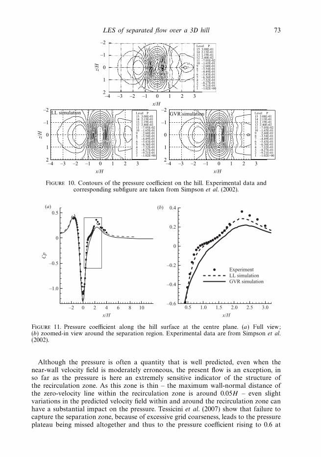
Figure 10. Contours of the pressure coefficient on the hill. Experimental data andcorresponding subfigure are taken from Simpson et al. (2002).
0.5 1.0 1.5 2.0 2.5 3.0–0.6
–0.4
–0.2
0
0.2
0.4
ExperimentLL simulationGVR simulation
(b)
x/H x/H
Cp
–2 0 2 4 6 8 10
–1.0
–0.5
0
0.5
(a)
Figure 11. Pressure coefficient along the hill surface at the centre plane. (a) Full view;(b) zoomed-in view around the separation region. Experimental data are from Simpson et al.(2002).
Although the pressure is often a quantity that is well predicted, even when thenear-wall velocity field is moderately erroneous, the present flow is an exception, inso far as the pressure is here an extremely sensitive indicator of the structure ofthe recirculation zone. As this zone is thin – the maximum wall-normal distance ofthe zero-velocity line within the recirculation zone is around 0.05H – even slightvariations in the predicted velocity field within and around the recirculation zone canhave a substantial impact on the pressure. Tessicini et al. (2007) show that failure tocapture the separation zone, because of excessive grid coarseness, leads to the pressureplateau being missed altogether and thus to the pressure coefficient rising to 0.6 at
74 M. Garcıa-Villalba, N. Li, W. Rodi and M. A. Leschziner
x/H x/H
y/H
0 0.2 0.4 0.6 0.8 1.0 1.2 1.4 1.6 1.8 2.0
0.2
0.4
0.6
0.8
1.0
1.2
x/H
y/H
0 0.2 0.4 0.6 0.8 1.0 1.2 1.4 1.6 1.8 2.0
0.2
0.4
0.6
0.8
1.0
1.2
0 0.2 0.4 0.6 0.8 1.0 1.2 1.4 1.6 1.8 2.0
0.2
0.4
0.6
0.8
1.0
1.2
1
LL simulation
Exp.
1
v = 0
1
GVR simulation
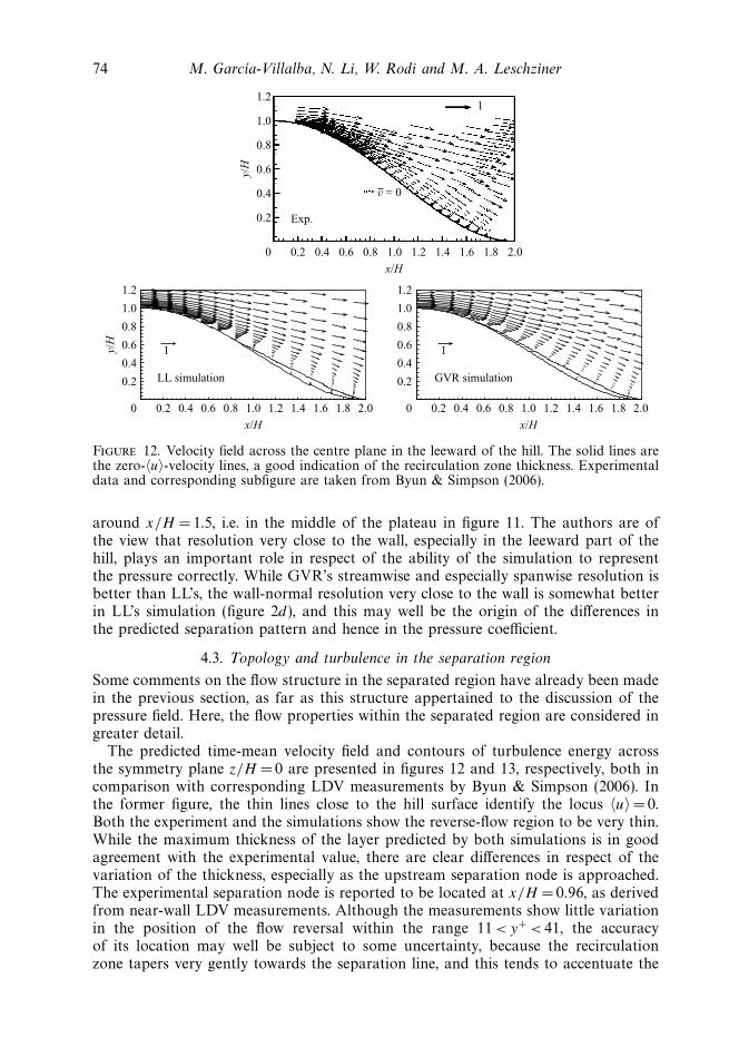
Figure 12. Velocity field across the centre plane in the leeward of the hill. The solid lines arethe zero-〈u〉-velocity lines, a good indication of the recirculation zone thickness. Experimentaldata and corresponding subfigure are taken from Byun & Simpson (2006).
around x/H = 1.5, i.e. in the middle of the plateau in figure 11. The authors are ofthe view that resolution very close to the wall, especially in the leeward part of thehill, plays an important role in respect of the ability of the simulation to representthe pressure correctly. While GVR’s streamwise and especially spanwise resolution isbetter than LL’s, the wall-normal resolution very close to the wall is somewhat betterin LL’s simulation (figure 2d), and this may well be the origin of the differences inthe predicted separation pattern and hence in the pressure coefficient.
4.3. Topology and turbulence in the separation region
Some comments on the flow structure in the separated region have already been madein the previous section, as far as this structure appertained to the discussion of thepressure field. Here, the flow properties within the separated region are considered ingreater detail.
The predicted time-mean velocity field and contours of turbulence energy acrossthe symmetry plane z/H = 0 are presented in figures 12 and 13, respectively, both incomparison with corresponding LDV measurements by Byun & Simpson (2006). Inthe former figure, the thin lines close to the hill surface identify the locus 〈u〉 =0.Both the experiment and the simulations show the reverse-flow region to be very thin.While the maximum thickness of the layer predicted by both simulations is in goodagreement with the experimental value, there are clear differences in respect of thevariation of the thickness, especially as the upstream separation node is approached.The experimental separation node is reported to be located at x/H = 0.96, as derivedfrom near-wall LDV measurements. Although the measurements show little variationin the position of the flow reversal within the range 11 <y+ < 41, the accuracyof its location may well be subject to some uncertainty, because the recirculationzone tapers very gently towards the separation line, and this tends to accentuate the

LES of separated flow over a 3D hill 75
x/H
y/H
0 0.2 0.4 0.6 0.8 1.0 1.2 1.4 1.6 1.8 2.0
0.2
0.4
0.6
0.8
1.0
1.2TKE
0.0460.0430.0390.0360.0330.0300.0260.0230.0200.0160.0130.0100.0070.0030.000
x/H
0 0.2 0.4 0.6 0.8 1.0 1.2 1.4 1.6 1.8 2.0
0.2
0.4
0.6
0.8
1.0
1.2TKE
0.0460.0430.0390.0360.0330.0300.0260.0230.0200.0160.0130.0100.0070.0030.000
x/H
y/H
0 0.2 0.4 0.6 0.8 1.0 1.2 1.4 1.6 1.8 2.0
0.2
0.4
0.6
0.8
1.0
1.2 TKE/Uref2
0.0460.0430.0390.0360.0330.0300.0260.0230.0200.0160.0130.0100.0070.0030.000
LL simulation GVR simulation
Figure 13. Turbulent kinetic energy distribution across the centre plane in the leeward of thehill. Experimental data and corresponding subfigure are taken from Byun & Simpson (2006).
consequence of near-wall-resolution limitations. LL’s separation point appears, on firstsight, to be in good agreement with the experimental value, while GVR’s locationappears to be too close to the hill crest, at around x/H ∼ 0.5. In fact, as shownlater, by reference to topology maps, both simulations predict very similar separationlocations at around x/H ∼ 0.3, i.e. substantially upstream of the experimental value.The difference between the simulations thus lies in the rate at which the thickness ofthe recirculation zone diminishes to zero towards the hill crest, LL’s recirculation zonebeing significantly thinner in the range x/H = 0.3–0.9. These differences in thicknessvariations might appear rather unimportant, but they have, in fact, a major impacton the pressure field, as noted in the previous section. Both simulations predictthe location of reattachment at around x/H ∼ 2, closely matching the experimentallocation.
It is appropriate to point out here that the thinness of the recirculation zonemakes its accurate capture, both experimentally and computationally, an extremelychallenging task. It needs to be appreciated that the separation pattern variessubstantially over time and space, to the extent that separation is intermittent, sothat the time-mean properties of the separated zone are likely to be very sensitiveto the turbulence dynamics of the entire flow, as well as to the precise mannerin which the turbulent inlet conditions are prescribed. More generally, this layer islikely to be extremely sensitive to very small variations in both the computationalor experimental conditions whatever their origin. As noted in the previous section,one possible contributor to the differences is the mesh density within the recirculationzone, especially the wall-normal density, which is somewhat higher in LL’s simulationin the region y/H < 0.02, as shown in figure 2(d).
Turbulence energy contours are shown in figure 13. One initially surprising aspectof the experimental observations is the presence of a patch of high turbulence energyjust downstream of the hill crest, around x/H ∼ 0.3, i.e. in a region well upstream of

76 M. Garcıa-Villalba, N. Li, W. Rodi and M. A. Leschziner
the recorded separation point x/H ∼ 0.9. As noted earlier, the simulations suggest incontrast that the area in which a high level of k occurs is around the separation line.Thus, the simulations bring to light the fact that the high-turbulence area is not inan attached region, but a consequence of the unsteady separation well upstream ofthe experimentally recorded position. The turbulence field of LL’s simulation showsespecially well the thin zone of high turbulence in the region 0.2 <x/H < 0.6. It willbe shown later that this region is also characterized by an especially high level ofproduction of turbulence energy near the surface, consistent with the thin separatedlayer.
The high level of turbulence arising in the separated shear layer as it evolves beyondx/H ∼ 0.8 is entirely in accord with expectation. This layer thickens progressively inthe downstream direction, and with it, the region of high turbulence energy alsobecomes more extensive. The GVR simulation predicts larger values of k than boththe LDV measurements and the LL simulation, and this provides a further indicationthat the recirculation region returned by the former simulation is somewhat excessive.As shown in the next section dealing with the wake, the GVR simulation also predictshigher values of k than the LL simulation in the wake region, well downstream ofreattachment, but in that case agreement of the GVR predictions with hot-wiremeasurements (Ma & Simpson 2005) of k, regarded as more accurate than the LDVdata at that location, is close and better than that achieved by LL’s simulation. Thiscould indicate some inconsistencies between the two sets of measurements, but couldalso be attributed to the inferior resolution of the LL simulation due to the coarsergrid it uses especially in the wake region.
The overall view conveyed by figures 12 and 13 is complemented by figure 14, whichshows profiles of mean and r.m.s. velocities as a function of the wall-normal distancein wall units, in the symmetry plane. Attention is drawn to the fact that the frictionvelocity used for normalization is at its reference value that prevails upstream of thehill at x/H = −4.0. Here, the comparison is made with the LDV data reported by Byun(2005). To this end, the Cartesian components of the computed velocity field in thesymmetry plane were projected onto the wall-tangential and wall-normal directions.Figure 14(a) shows the mean tangential velocity 〈ut〉 just upstream, x/H =0.18, ofthe (computed) separation location. At this location, the flow is observed to haveexperienced strong acceleration by the hill, the flow speed at the edge of the boundarylayer being roughly 30 % higher than Uref . Also, the boundary layer has becomevery thin at this location, its thickness being somewhat less than 100 wall units. Thiscompares with a boundary-layer thickness of δ = 0.5H upstream of the hill, whichcorresponds to approximately 2300 wall units. Figure 14(b) shows the same quantitydownstream of separation, in the recirculation region, x/H =1.31. At this location,the recirculation region is well established in both simulations and in the experiment,and it is several hundred wall units thick. Figures 14(c–d ) show profiles of thecorresponding r.m.s. velocities in the wall-tangential and normal directions. Upstreamof separation, the tangential fluctuations are significantly higher than the normalfluctuations, with the ratio being approximately 4 below y+ =50. At this location,high levels of fluctuations occur in the region below y+ = 100, corresponding tothe high strain rate observed in the associated velocity profile. In the recirculationregion, the tangential fluctuations are roughly twice the normal fluctuations and aredistributed across a broad layer extending to y+ ∼ 2000. The peak is attained aty+ ∼ 1000, which corresponds to the central part of the separated shear layer atthis location. In general, both simulations present a reasonable agreement with theexperimental data. The fluctuations predicted by GVR are somewhat higher than

LES of separated flow over a 3D hill 77
100 101 102 103
100 101 102 103
–0.2
0.25
0.20
0.15
0.10
0.05
0
0
0.2
0.4
0.6
0.8
1.0
1.2
1.4(a) (b)
(c) (d)
y+
100 101 102 103
0.25
0.20
0.15
0.10
0.05
0
y+
�u t
�/U
ref
100 101 102 103–0.2
0
0.2
0.4
0.6
0.8
1.0
1.2
1.4
u trm
s /U
ref,
u nrm
s /U
ref
Figure 14. (a–b) Mean tangential velocity 〈ut〉 as a function of y+. (c–d ) r.m.s. tangentialvelocity urms
t (upper curves) and r.m.s. normal velocity urmsn (lower curves) as a function of
y+. z/H =0. (a) and (c) Upstream of separation x/H =0.18. (b) and (d ) Downstream ofseparation x/H = 1.31. Solid lines, GVR; dashed lines, LL; symbols and experimental dataare from Byun (2005).
those predicted by LL, as expected from the contours of turbulent kinetic energydiscussed above.
The previous discussion (on figures 12–14) restricted itself to the flow in thesymmetry plane. A broader view of the three-dimensional structure of the meanflow is provided by streak-line maps across wall-parallel surfaces that cut throughthe separated zone at fixed wall-normal distances. Such maps projected onto thex–z plane are shown in figures 15–17 together with contours of turbulence energy.Figure 15 shows the results of LL, figure 16 shows the results of GVR and figure 17plots the measurements of Byun & Simpson (2006).
At the location closest to the wall, y+ ∼ 2, the predicted flow is very similar in bothsimulations with separation occurring almost along the same locus –x/H ∼ 0.3 at thecentreline. Reference to figure 12 brings out the fact that the reverse-flow layer isextremely thin near the wall, especially in LL’s simulation. Figure 17 suggests thatthe experimental separation line is well downstream of the computed line, but theuncertainties associated with this difference have already been noted. Farther awayfrom the wall, the zone of flow reversal progressively moves downstream in bothsimulations, but at a faster rate in the LL simulation, consistent with the fact that thethickness of the reverse-flow layer predicted by this simulation is lower. One of themain differences between the experimental and computational topology maps relates

78 M. Garcıa-Villalba, N. Li, W. Rodi and M. A. Leschziner
k: 0 0.009
(a)
2.0
1.5
1.0z/H
0.5
0 0.5 1.0 1.5 2.0
0.018 0.027 0.036 0.045
y+ ~ 2k: 0 0.009
(b)
2.0
1.5
1.0
0.5
0 0.5 1.0 1.5 2.0
0.018 0.027 0.036 0.045
y+ ~ 11k: 0 0.009
(c)
2.0
1.5
1.0
0.5
0 0.5 1.0 1.5 2.0
0.018 0.027 0.036 0.045
y+ ~ 40
k: 0 0.009
(d)
2.0
1.5
1.0z/H
0.5
0 0.5 1.0 1.5 2.0
0.018 0.027 0.036 0.045
y+ ~ 100k: 0 0.009
(e)
2.0
1.5
1.0
0.5
0 0.5 1.0 1.5 2.0
0.018 0.027 0.036 0.045
y+ ~ 180k: 0 0.009
( f )
2.0
1.5
1.0
0.5
0 0.5 1.0 1.5 2.0
0.018 0.027 0.036 0.045
y+ ~ 250
k: 0 0.009
(g)
2.0
1.5
1.0z/H
x/H x/H x/H
0.5
0 0.5 1.0 1.5 2.0
0.018 0.027 0.036 0.045
y+ ~ 330k: 0 0.009
(h)
2.0
1.5
1.0
0.5
0 0.5 1.0 1.5 2.0
0.018 0.027 0.036 0.045
y+ ~ 400k: 0 0.009
(i)
2.0
1.5
1.0
0.5
0 0.5 1.0 1.5 2.0
0.018 0.027 0.036 0.045
y+ ~ 600
Figure 15. Flow topology predicted by LL simulation. Colour represents turbulentkinetic energy.
to the structural variation with height close to the wall. The experiments show hardlyany change in the flow-reversal line in the layer 11<y+ < 41, while the simulationsnot only show the flow-reversal line to be well upstream of the experimental locus,but also indicate that the flow experiences significant wall-normal variations. In LL’ssimulation, the shift is somewhat larger, and this reflects the extreme thinness of thereverse-flow layer returned by this simulation in the upstream area. These differencesadd weight to the suggestion that resolution limitations in the experiment may wellhave prevented a proper representation of the near-wall flow and of the actualseparation line. Beyond y+ ∼ 180, flow reversal occurs broadly at the same positionin both simulations.
Both simulations return very similar features for the outer vortex that emanatesfrom the focal point seen in the topology map (figure 8b). Thus, at y+ ∼ 180, thecentre of this vortex is located roughly at x/H = 1.5, z/H =0.7, somewhat fartherdownstream than in the experiment where the centre is at x/H = 1.4. Significant

LES of separated flow over a 3D hill 79
k: 0 0.009 0.018 0.027 0.036 0.045 0 0.009 0.018 0.027 0.036 0.045 0 0.009 0.018 0.027 0.036 0.045
0 0.009 0.018 0.027 0.036 0.045 0 0.009 0.018 0.027 0.036 0.045 0 0.009 0.018 0.027 0.036 0.045
0 0.009 0.018 0.027 0.036 0.045 0 0.009 0.018 0.027 0.036 0.045 0 0.009 0.018 0.027 0.036 0.045
(a)
2.0
1.5
1.0z/H
0.5
0 0.5 1.0 1.5 2.0
y+ ~ 2 k: k:
(b)
2.0
1.5
1.0
0.5
0 0.5 1.0 1.5 2.0
y+ ~ 11(c)
1.5
2.0
1.0
0.5
0 0.5 1.0 1.5 2.0
y+ ~ 40
k:
(d)
2.0
1.5
1.0z/H
0.5
0 0.5 1.0 1.5 2.0
y+ ~ 100 k:
(e)
2.0
1.5
1.0
0.5
0 0.5 1.0 1.5 2.0
y+ ~ 180 k:
( f )
2.0
1.5
1.0
0.5
0 0.5 1.0 1.5 2.0
y+ ~ 250
k:
(g)
2.0
1.5
1.0z/H
x/H x/H x/H
0.5
0 0.5 1.0 1.5 2.0
y+ ~ 330 k:
(h)
2.0
1.5
1.0
0.5
0 0.5 1.0 1.5 2.0
y+ ~ 400 k:
(i)
2.0
1.5
1.0
0.5
0 0.5 1.0 1.5 2.0
y+ ~ 600
Figure 16. Flow topology predicted by GVR simulation. Colour represents turbulentkinetic energy.
differences arise, however, in respect of the secondary vortex close to the centreline.It is recalled that this vortex (or pair of vortices) evolves from the forward separationnode, as a consequence of the transverse pressure gradient-inducing motion along theseparation line towards the centre plane, between the two saddle points on that line(figure 8b). The vorticity accumulating at the separation node, from both sides of thecentreline, has to be shed away from the wall. This process occurs in both simulations,and it is shown later that this vorticity is contained, in almost equal measure, in bothpredicted wakes. However, it is clear that the secondary vortex is more pronouncedin GVR’s simulation. This may be partly due to LL’s lower resolution away from thewall, but it also seems to be linked, to a considerable extent, to the differences in thethickness of the reverse-flow layer and the rate at which it changes with streamwisedistance. Initially, and in line with the slow increase in Cp (figure 11b), GVR’s resultsshow a faster thickening of the reverse-flow region. Beyond x/H � 1, the positionreverses due to the penetration of forward-moving fluid into the reverse-flow region

80 M. Garcıa-Villalba, N. Li, W. Rodi and M. A. Leschziner
4.50E-024.21E-023.91E-023.62E-023.33E-023.04E-022.74E-022.45E-022.16E-021.88E-021.57E-021.28E-029.86E-036.93E-034.00E-03
TKE/Uref2
0.2
–2.0(a)
–1.5
z/H
z/H
x/H x/H
–1.0
–0.5
0 0.5 1.0
y+L0 = 11
1.5 2.0
4.50E-024.21E-023.91E-023.62E-023.33E-023.04E-022.74E-022.45E-022.16E-021.88E-021.57E-021.28E-029.86E-036.93E-034.00E-03
TKE/Uref2
0.2
–2.0(b)
–1.5
–1.0
–0.5
0 0.5 1.0
y+L0 = 41
1.5 2.0
4.50E-024.21E-023.91E-023.62E-023.33E-023.04E-022.74E-022.45E-022.16E-021.88E-021.57E-021.28E-029.86E-036.93E-034.00E-03
TKE/Uref2
0.2
–2.0(c)
–1.5
–1.0
–0.5
0 0.5 1.0
y+L0 = 200
1.5 2.0
4.50E-024.21E-023.91E-023.62E-023.33E-023.04E-022.74E-022.45E-022.16E-021.88E-021.57E-021.28E-029.86E-036.93E-034.00E-03
TKE/Uref2
0.2
–2.0(d)
–1.5
–1.0
–0.5
0 0.5 1.0
y+L0 = 578
1.5 2.0
Figure 17. Flow topology (lines) and turbulent kinetic energy (colour) measured by Byun &Simpson (2006).
associated with the formation of the secondary vortex. Thus, in this region, LL’sreverse-flow layer thickens more rapidly and Cp develops more of a plateau. Beyondx/H � 1.2–1.3, both simulations return virtually the same thickness. Based on theseobservations, it is conjectured that the secondary vortical structures predicted byGVR’s simulation are likely to be too large in size and intensity.
The contours of turbulent kinetic energy in figures 15–17, overlaid onto the flowmaps, are consistent with the principal observation derived from figure 13, namely thatGVR’s simulation predicts higher values of k than both LL’s and the experimentallevels, suggesting that the extent and intensity of the separation process predictedby GVR’s simulation is at least slightly excessive. In general, high levels of k areobserved ahead and around the flow-reversal line, as well as on either side of therecirculation zone. The levels within the reverse-flow region are lower, reflecting thedamping exerted by the wall on the upstream-flowing near-wall layer. At y+ = 40,there is a spanwise patch of elevated k at around x/H = 0.3–0.4, which is observed inboth simulations and the experiment. In both simulations, this patch is located justupstream of the flow-reversal line, while in the experiment, this line is located muchfarther downstream at around x/H ∼ 0.9. The patch may be interpreted to reflectthe highly unsteady nature of the separation process, in which the stagnation line aty+ ∼ 11 extends, at times, well upstream of its mean location x/H ∼ 0.5. The focus
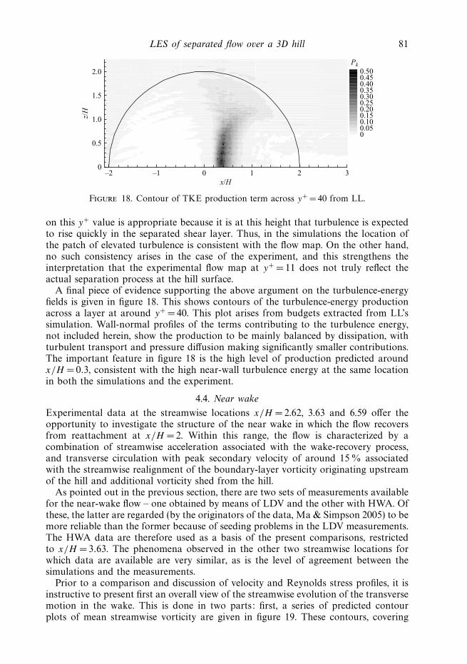
LES of separated flow over a 3D hill 81
x/H
z/H
–2 –1 0 1 2 30
0.5
1.0
1.5
2.0 0.500.450.400.350.300.250.200.150.100.050
Pk
Figure 18. Contour of TKE production term across y+ = 40 from LL.
on this y+ value is appropriate because it is at this height that turbulence is expectedto rise quickly in the separated shear layer. Thus, in the simulations the location ofthe patch of elevated turbulence is consistent with the flow map. On the other hand,no such consistency arises in the case of the experiment, and this strengthens theinterpretation that the experimental flow map at y+ = 11 does not truly reflect theactual separation process at the hill surface.
A final piece of evidence supporting the above argument on the turbulence-energyfields is given in figure 18. This shows contours of the turbulence-energy productionacross a layer at around y+ = 40. This plot arises from budgets extracted from LL’ssimulation. Wall-normal profiles of the terms contributing to the turbulence energy,not included herein, show the production to be mainly balanced by dissipation, withturbulent transport and pressure diffusion making significantly smaller contributions.The important feature in figure 18 is the high level of production predicted aroundx/H = 0.3, consistent with the high near-wall turbulence energy at the same locationin both the simulations and the experiment.
4.4. Near wake
Experimental data at the streamwise locations x/H = 2.62, 3.63 and 6.59 offer theopportunity to investigate the structure of the near wake in which the flow recoversfrom reattachment at x/H =2. Within this range, the flow is characterized by acombination of streamwise acceleration associated with the wake-recovery process,and transverse circulation with peak secondary velocity of around 15 % associatedwith the streamwise realignment of the boundary-layer vorticity originating upstreamof the hill and additional vorticity shed from the hill.
As pointed out in the previous section, there are two sets of measurements availablefor the near-wake flow – one obtained by means of LDV and the other with HWA. Ofthese, the latter are regarded (by the originators of the data, Ma & Simpson 2005) to bemore reliable than the former because of seeding problems in the LDV measurements.The HWA data are therefore used as a basis of the present comparisons, restrictedto x/H = 3.63. The phenomena observed in the other two streamwise locations forwhich data are available are very similar, as is the level of agreement between thesimulations and the measurements.
Prior to a comparison and discussion of velocity and Reynolds stress profiles, it isinstructive to present first an overall view of the streamwise evolution of the transversemotion in the wake. This is done in two parts: first, a series of predicted contourplots of mean streamwise vorticity are given in figure 19. These contours, covering

82 M. Garcıa-Villalba, N. Li, W. Rodi and M. A. Leschziner
1.0
(a) (b)
x/H = 0
0.5
0
1.0
0.5
0–2.0 –1.5 –1.0
–0.50 –0.25 0 0.25 0.50
–0.5 0 0 0.5 1.0 1.5 2.0
y/H
1.0
x/H = 0.4
0.5
0
1.0
0.5
0–2.0 –1.5 –1.0 –0.5 0 0 0.5 1.0 1.5 2.0
y/H
1.0
x/H = 1.0
0.5
0
1.0
0.5
0–2.0 –1.5 –1.0 –0.5 0 0 0.5 1.0 1.5 2.0
y/H
1.0
x = 1.25H
0.5
0
1.0
0.5
0–2.0 –1.5
1 2
3
4
–1.0 –0.5 0 0 0.5 1.0 1.5 2.0
y/H
1.0
x = 1.75H
0.5
0
1.0
0.5
0–2.0 –1.5 –1.0 –0.5 0 0 0.5 1.0 1.5 2.0
y/H
1.0
x = 2.5H
0.5
0
1.0
0.5
0–2.0 –1.5 –1.0 –0.5 0 0 0.5 1.0 1.5 2.0
y/H
z/H z/H
Figure 19. Mean streamwise vorticity at several transverse planes. (a) LL; (b) GVR. Notethat the streamwise vorticity field is antisymmetric with respect to the symmetry plane.

LES of separated flow over a 3D hill 83
1.0
(a) (b)
0.8
0.6
0.4
0.2
0–2.5 –2.0 –1.5 –1.0 –0.5 0 0.5
0.040
0.001
0.010
0.050
0.055
0.040
0.001
0.002
0.010
0.005
0.020
0.030
0.0200.005
0.001
0.0020.005
0.0100.005
0.005
0.035
0.005
0.030
0.001 0
0.020 0.0050.002
1.0 1.5 2.0 2.5
1.2x/H = 2
x/H = 3
x/H = 5
1.0
0.8
0.6
0.4
0.2
0
y/H
1.0
0.8
0.6
0.4
0.2
0–2.5 –2.0 –1.5 –1.0 –0.5 0 0.5 1.0 1.5 2.0 2.5
1.2
1.0
0.8
0.6
0.4
0.2
0
y/H
1.0
0.8
0.6
0.4
0.2
0–2.5 –2.0 –1.5 –1.0 –0.5 0 0.5 1.0 1.5 2.0 2.5
1.2
1.0
0.8
0.6
0.4
0.2
0
y/H
z/H z/H
0.015
Figure 20. (a) Secondary motions at x/H = 2, 3 and 5. (b) Turbulent kinetic energy.Simulation GVR.
the streamwise stretch 0<x/H < 2.5, allow the formation of the wake structure to betraced to specific processes occurring in the leeward portion of the hill, specificallyto features discussed earlier by reference to figures 15–17. Second, figure 20 showsthe evolution of the transverse motion and turbulence energy farther downstream,covering the streamwise stretch 2<x/H < 5. Figure 19 is a composite of resultsarising from both simulations: LL’s in figure 19a, and GVR’s in figure 19b (thecolour reversal across the centreline reflects the change in the sign of the vorticity).Both sets show a remarkable degree of similarity. Most informative is the evolutionof the flow beyond x/H = 1.0. With attention focused on the left-hand side set ofplots (figure 19a), four distinct regions may be recognized, identified numerically inthe plot for x = 1.25H : an outer red region, 1, of positive vorticity lying at somedistance above the wall; an outer blue region, 2, of negative vorticity close to thewall; an inner red region, 3, of positive vorticity above the wall; and a very thinblue inner layer, 4, of negative vorticity very close to the wall. The origin of the fourregions are, respectively, as follows: 1, the vorticity of the boundary layer upstreamof the hill, having been reoriented towards the streamwise direction; 2, the vorticityshed from the primary focal point in the separation zone, 3, the vorticity shed fromthe separation node, reflected by the secondary spiral close to the centre plane; and4, the vorticity in the very thin separated zone.
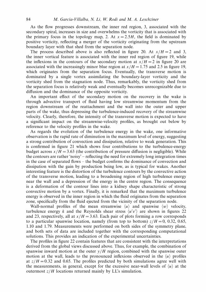
84 M. Garcıa-Villalba, N. Li, W. Rodi and M. A. Leschziner
As the flow progresses downstream, the inner red region, 3, associated with thesecondary spiral, increases in size and overwhelms the vorticity that is associated withthe primary focus in the topology map, 2. At x = 2.5H , the field is dominated bypositive vorticity, reflecting a merger of the vorticity originating from the upstreamboundary layer with that shed from the separation node.
The process described above is also reflected in figure 20. At x/H =2 and 3,the inner vortical feature is associated with the inner red region of figure 19, whilethe inflexions in the contours of the secondary motion at x/H = 2 in figure 20 areassociated with the increasingly minor blue region at x/H = 1.75 and 2.5 in figure 19,which originates from the separation focus. Eventually, the transverse motion isdominated by a single vortex assimilating the boundary-layer vorticity and thevorticity shed from the stagnation node. Thus, remarkably, the vorticity shed fromthe separation focus is relatively weak and eventually becomes unrecognizable due todiffusion and the dominance of the opposite vorticity.
An important effect of the secondary motion on the recovery in the wake isthrough advective transport of fluid having low streamwise momentum from theregion downstream of the reattachment and the wall into the outer and upperparts of the wake, thus depressing the turbulence-induced recovery of the streamwisevelocity. Clearly, therefore, the intensity of the transverse motion is expected to havea significant impact on the streamwise-velocity profiles, as brought out below byreference to the velocity profiles in the wake.
As regards the evolution of the turbulence energy in the wake, one informativeobservation is the rapid rate of diminution in the maximum level of energy, suggestinga strong contribution of convection and dissipation, relative to weak generation. Thisis confirmed in figure 21 which shows four contributions to the turbulence-energybudget across x/H =3.63 (the contribution of pressure diffusion is negligible). Whilethe contours are rather ‘noisy’ – reflecting the need for extremely long integration timesin the case of separated flows – the budget confirms the dominance of convection anddissipation with the gain by production being low, as is typical for wakes. Anotherinteresting feature is the distortion of the turbulence contours by the convective actionof the transverse motion, leading to a broadening region of high turbulence energynear the wall and a depression of the energy in the centre region. The consequenceis a deformation of the contour lines into a kidney shape characteristic of strongconvective motion by a vortex. Finally, it is remarked that the maximum turbulenceenergy is observed in the inner region in which the fluid originates from the separationzone, specifically from the fluid ejected from the vicinity of the separation node.
Wall-normal profiles of the mean streamwise 〈u〉 and spanwise 〈w〉 velocity,turbulence energy k and the Reynolds shear stress 〈u′v′〉 are shown in figures 22and 23, respectively, all at x/H = 3.63. Each pair of plots forming a row correspondsto a particular spanwise location, namely (from top to bottom) z/H = 0, 0.32, 0.65,1.10 and 1.79. Measurements were performed on both sides of the symmetry plane,and both sets of data are included together with the corresponding computationalsolutions. This provides an indication of the experimental uncertainties.
The profiles in figure 22 contain features that are consistent with the interpretationsderived from the global views discussed above. Thus, for example, the combination ofspanwise inward motion at the outer y/H region, combined with the spanwise outermotion at the wall, leads to the pronounced inflexions observed in the 〈u〉 profilesat z/H = 0.32 and 0.65. The profiles predicted by both simulations agree well withthe measurements, in general, except for the excessive near-wall levels of 〈u〉 at theoutermost z/H locations returned mainly by LL’s simulation.

LES of separated flow over a 3D hill 85
0.022
0.0100.0080.0060.0040.0020–0.002–0.004–0.006–0.008–0.010
0.0200.0180.0160.0140.0120.0100.0080.0060.0040.002
0.6
TKE
0.4
y/H
z/H
0.2
0–1.2 –1.0 –0.8 –0.6 –0.4 –0.2 0
0.6
0.4
Convection
Turbulenttransport
Dissipation(from balance)
Production
y/H
y/H
0.2
0–1.2 –1.0 –0.8 –0.6 –0.4 –0.2 0
0.6
0.4
0.2
0–1.2 –1.0 –0.8 –0.6 –0.4 –0.2 0
0.6
0.4
z/H z/H
0.2
0–1.2 –1.0 –0.8 –0.6 –0.4 –0.2 0
0.6
0.4
0.2
0–1.2 –1.0 –0.8 –0.6 –0.4 –0.2 0
Figure 21. Contour of TKE budget in wake plane x/H = 3.63 from LL.
Profiles for k and 〈u′v′〉 are shown in figure 23. As noted earlier, when discussing thestructure of the separation region, LL’s simulation generally predicts lower levels of k
than GVR’s simulation. While this was in accord with the experimental observations inthe recirculation zone, better agreement is achieved in the wake by GVR’s simulation,which is very good, overall. The decrease of the level of k and 〈u′v′〉 with increasingspanwise position is well captured by both simulations. Attention is drawn to thefact that the maximum level of k does not occur in the symmetry plane but aroundz/H = 0.32. Reference to figure 20 shows, consistently, that the maximum turbulenceenergy at x/H = 3.0 indeed lies at around z/H = 0.3, and this is probably due totransport of highly turbulent fluid from the separated region into this part of thewake, suggested by the streaklines identifying the transverse motion. The somewhattoo low level of turbulence activity returned by LL’s simulation and certain defects inthe 〈u〉 profile such as the near-wall bulge are likely to be due to the substantially lowerresolution provided by LL’s coarser grid in the wake, especially in outer spanwiseregions.
5. Analysis of the instantaneous flow and spectra5.1. Instantaneous flow
Any turbulent separated flow features high-intensity, highly unsteady, large-scalemotions that render the instantaneous state drastically different from its time-averaged

86 M. Garcıa-Villalba, N. Li, W. Rodi and M. A. Leschziner
0 0.2 0.4 0.6 0.8 1.0
0.2
0.4
0.6
0.8
1.0
(a) (b)
0
0.2
0.4
0.6
0.8
1.0y/
H
–0.10 –0.05 0 0.05 0.10
0 0.2 0.4 0.6 0.8 1.0
0.2
0.4
0.6
0.8
1.0
0
0.2
0.4
0.6
0.8
1.0
y/H
–0.10 –0.05 0 0.05 0.10
0 0.2 0.4 0.6 0.8 1.0
0.2
0.4
0.6
0.8
1.0
0
0.2
0.4
0.6
0.8
1.0
y/H
–0.10 –0.05 0 0.05 0.10
0 0.2 0.4 0.6 0.8 1.0
0.2
0.4
0.6
0.8
1.0
0
0.2
0.4
0.6
0.8
1.0
y/H
–0.10 –0.05 0 0.05 0.10
0 0.2 0.4 0.6 0.8 1.0
0.2
0.4
0.6
0.8
1.0
0
0.2
0.4
0.6
0.8
1.0
y/H
–0.10 –0.05 0 0.05 0.10
�u�/Uref �w�/Uref
Figure 22. Profiles of (a) streamwise 〈u〉 and (b) spanwise mean velocity 〈w〉 at x/H = 3.63.From top to bottom, z/H = 0, 0.32, 0.65, 1.10 and 1.79. Symbols, experiments; solid line, GVR;dashed line, LL. Experimental data are from Ma & Simpson (2005).

LES of separated flow over a 3D hill 87
0 0.01 0.02
0.2
0.4
0.6
0.8
1.0
(a) (b)
0
0.2
0.4
0.6
0.8
1.0
y/H
–0.008 –0.004 0
0 0.01 0.02
0.2
0.4
0.6
0.8
1.0
0
0.2
0.4
0.6
0.8
1.0
y/H
–0.008 –0.004 0
0 0.01 0.02
0.2
0.4
0.6
0.8
1.0
0
0.2
0.4
0.6
0.8
1.0
y/H
–0.008 –0.004 0
0 0.01 0.02
0.2
0.4
0.6
0.8
1.0
0
0.2
0.4
0.6
0.8
1.0
y/H
–0.008 –0.004 0
0 0.01 0.02
0.2
0.4
0.6
0.8
1.0
0
0.2
0.4
0.6
0.8
1.0
y/H
–0.008 –0.004 0
k/U 2ref �u′v′�/U 2
ref
Figure 23. Profiles of (a) turbulent kinetic energy k and (b) Reynolds shear stress 〈u′v′〉 atx/H =3.63. Here, z-positions and styles are as in figure 22. Experimental data are from Ma& Simpson (2005).
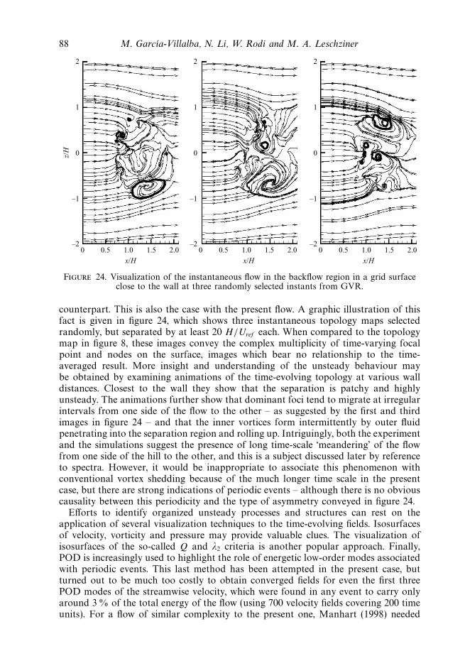
88 M. Garcıa-Villalba, N. Li, W. Rodi and M. A. Leschziner
2
1
0
–1
–20 0.5 1.0
x/H
1.5 2.0
2
1
0
–1
–20 0.5 1.0
x/H
1.5 2.0
2
1
0
–1
–20 0.5 1.0
x/H
z/H
1.5 2.0
Figure 24. Visualization of the instantaneous flow in the backflow region in a grid surfaceclose to the wall at three randomly selected instants from GVR.
counterpart. This is also the case with the present flow. A graphic illustration of thisfact is given in figure 24, which shows three instantaneous topology maps selectedrandomly, but separated by at least 20 H/Uref each. When compared to the topologymap in figure 8, these images convey the complex multiplicity of time-varying focalpoint and nodes on the surface, images which bear no relationship to the time-averaged result. More insight and understanding of the unsteady behaviour maybe obtained by examining animations of the time-evolving topology at various walldistances. Closest to the wall they show that the separation is patchy and highlyunsteady. The animations further show that dominant foci tend to migrate at irregularintervals from one side of the flow to the other – as suggested by the first and thirdimages in figure 24 – and that the inner vortices form intermittently by outer fluidpenetrating into the separation region and rolling up. Intriguingly, both the experimentand the simulations suggest the presence of long time-scale ‘meandering’ of the flowfrom one side of the hill to the other, and this is a subject discussed later by referenceto spectra. However, it would be inappropriate to associate this phenomenon withconventional vortex shedding because of the much longer time scale in the presentcase, but there are strong indications of periodic events – although there is no obviouscausality between this periodicity and the type of asymmetry conveyed in figure 24.
Efforts to identify organized unsteady processes and structures can rest on theapplication of several visualization techniques to the time-evolving fields. Isosurfacesof velocity, vorticity and pressure may provide valuable clues. The visualization ofisosurfaces of the so-called Q and λ2 criteria is another popular approach. Finally,POD is increasingly used to highlight the role of energetic low-order modes associatedwith periodic events. This last method has been attempted in the present case, butturned out to be much too costly to obtain converged fields for even the first threePOD modes of the streamwise velocity, which were found in any event to carry onlyaround 3 % of the total energy of the flow (using 700 velocity fields covering 200 timeunits). For a flow of similar complexity to the present one, Manhart (1998) needed

LES of separated flow over a 3D hill 89
t = 112.50
0
1
4
2
0z
yx
t = 127.25
0
0
1
–1
–1
4
2
0z
yx
t = 218.25
1
4
2
0z
yx
Figure 25. Visualization of the instantaneous flow from GVR. Blue, isosurface of streamwisevelocity fluctuations u − 〈u〉 = −0.25. Red, isosurface of streamwise velocity fluctuationsu − 〈u〉 = 0.25. White, isosurface of pressure fluctuations p − 〈p〉 = −0.06.
over 3000 fields to obtain converged modes. The approach taken here for elucidatingstructural features was to juxtapose isosurfaces of pressure with streamwise velocityfluctuations. This turns out to be instructive in so far as it brings out some interestingrelationships between streamwise velocity streaks and hairpin-like vortical structuresshed from the surface.
Figure 25 shows three such visualizations selected so as to bring out salient features.The plots contain three groups of isosurfaces. Two represent streamwise velocity

90 M. Garcıa-Villalba, N. Li, W. Rodi and M. A. Leschziner
fluctuations, u − 〈u〉 =0.25 (red) and −0.25 (blue), and the third shows (light grey)pressure fluctuations p − 〈p〉 = −0.06.
It is well known that coherent structures are associated with local minima of thepressure field (Jeong & Hussain 1995; Dubief & Delcayre 2000). Previous studies(Frohlich et al. 2005; Garcıa-Villalba, Frohlich & Rodi 2006) have demonstrated thatthe field of pressure fluctuations is a more effective indicator of coherent structuresthan the more commonly used instantaneous pressure. This is because isosurfacesof the latter are influenced by the spatially variable average pressure field, which isunrelated to instantaneous structures. This is avoided when 〈p〉 is subtracted fromthe instantaneous value. It might be presumed that vorticity contours, the λ2 criterionor the Q criterion (Jeong & Hussain 1995) would be preferable. However, in thepresent flow, the Reynolds number is relatively high, in which case intense small-scalevortical structures captured by these criteria tend to obscure the large-scale vorticalstructures of primary interest. Figure 25 (and corresponding animations) shows thatin the wake, distinct, large-scale, elongated regions of flow moving faster than themean flow (red) and more slowly than the mean (blue) are formed. These regionsare irregular in the sense that within some periods of time only one of each type ispresent, while at other times, both occur together, typically one on either side of thehill. Any one of the flow conditions lasts, typically, for several time units before it isconvected away or decays. There is no particular frequency to their occurrence, asshown below by reference to spectra of velocity fluctuations in this zone.
Coherent structures (light-grey) are observed to form in the leeward of the hill andare convected downstream. Many of them have the shape of a hairpin vortex, andthey are rapidly deformed by the high level of turbulence around them. The presenceof hairpin-shaped vortices in the flow behind a hill is not unexpected. Acarlar &Smith (1987) generated such vortices experimentally in a laminar boundary layerobstructed by a hemisphere. Moreover, Lardeau, Tessicini & Leschziner (2007) show,by way of highly resolved LES, that hairpin vortices arise when the present hill issubjected to a boundary layer at low Reynolds numbers. However, the pattern hereis more complex because the boundary layer is fully turbulent and the Reynoldsnumber is about 100 times larger.
It is interesting to note that the vortical structures ‘ride’ preferentially on the low-speed regions. In a sense, this scenario is similar to that of vortex packets described byAdrian (2007, figure 12) in turbulent boundary layers. Here, however, the hairpin-likestructures cover the whole shear-layer thickness.
5.2. Spectra
Time signals of the flow at several locations have been recorded in GVR’s simulationover a period of about 200 H/Uref . From these, spectra were determined by usinga Fourier transform with a Hamming window (Oppenheim & Schafer 1989), andsegments of length 4096 (standard spectrum) and 1024 (pre-multiplied spectrum),spanning a length of 37.1 and 9.3 H/Uref , respectively. The signal was decomposed intoseveral overlapping segments over which averaging was performed. These parameterswere selected so as to obtain a compromise between the smoothness of the spectrumand the width of the frequency window covered. In particular, it was necessaryto reduce the length of the segments for the pre-multiplied spectra because they arerepresented in a linear-log form, which tends to accentuate high-frequency oscillationsrelative to the log-log form.
In the experiment of Ma & Simpson (2005), time signals were recorded in thesymmetry plane at x/H = 3.63 and at various heights. Here, only the location

LES of separated flow over a 3D hill 91
10–4 10–2 100 10210–7
10–6
10–5
10–4
10–3
10–2
10–1
100(a) (b)
fH/Uref
E11
10–4 10–2 100 10210–7
10–6
10–5
10–4
10–3
10–2
10–1
100
f H/Uref
E33
ExpLES
ExpLES
Figure 26. Comparison of power spectra of velocity fluctuations between GVR andexperimental data from Ma & Simpson (2005). x/H =3.63, y/H = 0.358, z/H = 0.(a) Streamwise velocity spectra; (b) spanwise velocity spectra. The dashed line has a −5/3slope.
y/H = 0.36 is compared to the simulation, because this is roughly in the middle of theboundary layer where the turbulent kinetic energy is maximum (figure 23). Agreementat other heights is similar in both qualitative and quantitative terms. Figure 26 showsthe power spectrum of streamwise, E11, and spanwise, E33, velocity fluctuations. Thefrequency range in the experiment is wider because its duration, in real time, is 2–3orders of magnitude longer than the interval covered by the simulation. At the high-frequency end of the spectrum, the decay returned by the simulation is faster than thatin the experiment. For frequencies higher than f ∼ 6Uref /H , there is some piling-upof energy, and the spectrum is slightly overpredicted by the simulation. This may be aconsequence of numerical noise, which is introduced by the numerical scheme at thesmallest resolved scale, thus contaminating the high-frequency end of the spectrum.Apart from this sub-range, agreement between experiment and simulation is very goodover at least two decades in f , including the region with a −5/3 slope. It is relevantto point out that no pronounced peak is observed in the spectra, which demonstratesthat the introduction of the periodic inflow with frequency finf = 0.556Uref /H (§ 3.3)does not have an adverse influence on the region of interest.
The power spectrum does not provide insight into how much energy is containedwithin a given frequency range – specifically on how much energy is containedin the very low-frequency range that is not properly represented in the LES. Thisdeficiency can be addressed by constructing the pre-multiplied spectrum f E11(f E33),which measures the streamwise (spanwise) kinetic energy contained in a logarithmicfrequency interval centred at f (del Alamo & Jimenez 2003). The pre-multipliedspectra are displayed in figure 27. This representation clearly shows that a non-negligible amount of energy is contained in low-frequency modes of the streamwisevelocity component, but this does not apply to the spanwise component. The pre-multiplied spectra also show, more clearly than the power spectra, the pile-up ofenergy at the high-frequency end.
As noted above, the pre-multiplied spectrum derived from GVR’s simulation wasconstructed by splitting the time signal into segments of length 9.3 H/Uref andoverlapping them to enhance smoothness. Although it appears from figure 27 thatthe simulation does not cover the low-frequency peak at all, this is an artefact of
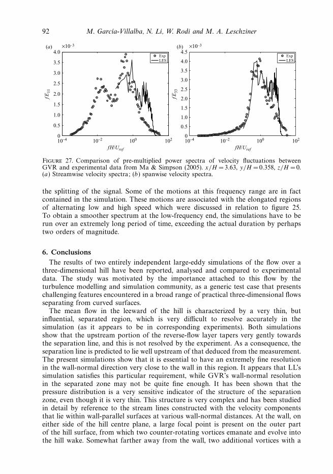
92 M. Garcıa-Villalba, N. Li, W. Rodi and M. A. Leschziner
10–4 10–2 100 1020
0.5
1.0
1.5
2.0
2.5
3.0
3.5
4.0(b)(a) ×10–3
fH/Uref
fE11
10–4 10–2 100 1020
1.0
0.5
1.5
2.0
2.5
3.0
3.5
4.0
4.5×10⁻³
fH/Uref
fE33
ExpLES
ExpLES
Figure 27. Comparison of pre-multiplied power spectra of velocity fluctuations betweenGVR and experimental data from Ma & Simpson (2005). x/H = 3.63, y/H = 0.358, z/H = 0.(a) Streamwise velocity spectra; (b) spanwise velocity spectra.
the splitting of the signal. Some of the motions at this frequency range are in factcontained in the simulation. These motions are associated with the elongated regionsof alternating low and high speed which were discussed in relation to figure 25.To obtain a smoother spectrum at the low-frequency end, the simulations have to berun over an extremely long period of time, exceeding the actual duration by perhapstwo orders of magnitude.
6. ConclusionsThe results of two entirely independent large-eddy simulations of the flow over a
three-dimensional hill have been reported, analysed and compared to experimentaldata. The study was motivated by the importance attached to this flow by theturbulence modelling and simulation community, as a generic test case that presentschallenging features encountered in a broad range of practical three-dimensional flowsseparating from curved surfaces.
The mean flow in the leeward of the hill is characterized by a very thin, butinfluential, separated region, which is very difficult to resolve accurately in thesimulation (as it appears to be in corresponding experiments). Both simulationsshow that the upstream portion of the reverse-flow layer tapers very gently towardsthe separation line, and this is not resolved by the experiment. As a consequence, theseparation line is predicted to lie well upstream of that deduced from the measurement.The present simulations show that it is essential to have an extremely fine resolutionin the wall-normal direction very close to the wall in this region. It appears that LL’ssimulation satisfies this particular requirement, while GVR’s wall-normal resolutionin the separated zone may not be quite fine enough. It has been shown that thepressure distribution is a very sensitive indicator of the structure of the separationzone, even though it is very thin. This structure is very complex and has been studiedin detail by reference to the stream lines constructed with the velocity componentsthat lie within wall-parallel surfaces at various wall-normal distances. At the wall, oneither side of the hill centre plane, a large focal point is present on the outer partof the hill surface, from which two counter-rotating vortices emanate and evolve intothe hill wake. Somewhat farther away from the wall, two additional vortices with a

LES of separated flow over a 3D hill 93
sense of rotation opposite to that of the outer ones develop close to the centre plane.The latter originate from the separation node that is at the apex of the separationline on the centre plane. Reattachment occurs roughly at the leeward foot of the hill,and both simulations return virtually the same reattachment location.
The wake is characterized by a combination of streamwise acceleration andtransverse circulation. The former is associated with the wake-recovery process andthe latter with secondary motions originating from a combination of the streamwiserealignment of the vorticity in the upstream boundary layer and substantial additionalvorticity generated at the hill surface. The latter is an amalgam of vorticity componentsof opposite sense originating from the outer focal points and from the separation nodeat the apex of the separation line. As the wake evolves, the vortices shed from theouter focal points are overwhelmed, through a diffusive mechanism, by the vorticityshed from the separation node. As a result, the latter vortices dictate the sense ofrotation of the secondary motion in the wake. The influence of wall-normal resolutionin the wake, relative to streamwise and spanwise resolution, is weaker than in theseparated region, and in this area GVR’s grid is distinctly superior to LL’s grid, thusyielding a more faithful representation of the wake structure.
The main characteristics of the flow are well reproduced by both simulations, andthere is a gratifying level of agreement between them in respect of the dimensions ofthe separation zone, the mean velocity, the Reynolds stresses, the principal topologicalfeatures and the wake structure – the last reproduced especially well by GVR’ssimulation. There are, however, also some non-negligible differences between them, aswell as between both simulations and the experiment. The most important differencein the latter category concerns the topological features observed at the wall. In theexperiment (Byun & Simpson 2006), two foci and one saddle point were observedin the separation region. The region of reattachment could not be measured, andByun & Simpson conjectured that, to fulfil the topological rules, the reattachmentregion should contain one reattachment node and two additional saddle points (i.e.three nodes and three saddle points, in total). Both simulations return a differenttopology, featuring four nodes and four saddle points. Furthermore, it has beenshown that this is consistent with the predicted development of the mean streamwisevorticity in the wake, which is in good agreement with the HWA measurementsof Ma & Simpson (2005). This observation supports the validity of the topologypredicted by the simulations. A second difference relative to the experiments concernsthe prediction of the location of the separation line. The origin of the unexpectedexperimental observation of a patch of high turbulence energy well upstream of theexperimentally deduced separation region has been elucidated by the simulations.These demonstrate that the area of high turbulence energy is a consequence of thehighly unsteady separation process, resulting in a very thin time-mean reverse-flowlayer extending well upstream of the location determined experimentally. Hence, thepatch of high turbulence energy, shown to be a consequence of high turbulenceproduction, is closely associated with the separation process.
As regards differences between the two simulations, the most important relatesto the wall pressure in the separation region. A close examination of the flow inthe separated region has revealed that these differences originate from the extremesensitivity of the pressure gradient to the variation of the wall-normal thickness of thereverse-flow layer. This sensitivity highlights the extreme resolution challenges posedby three-dimensional separation from curved surfaces.
Although the study has targeted primarily the resolution of the mean-flowcharacteristics, some useful observations have also been made in respect of unsteady
94 M. Garcıa-Villalba, N. Li, W. Rodi and M. A. Leschziner
features and processes. It has been shown that, while the separation region is highlyunsteady, the flow is separated at all times at least over some parts of the surface.Based on the measurement of bimodal velocity PDF’s, Byun (2005) speculated onthe possibility that the separation is intermittent, involving a switching betweendetached and attached flow. This scenario is not supported by the simulations.Another interesting feature observed in the simulations is the presence in the wakeof alternating regions of fluid in which the streamwise velocity is higher or lowerthan the mean. Associated with the low-speed regions, coherent structures have beenidentified, some having the form of hairpin vortices. These events are very energetic,as is evident in time signals of the velocity recorded in the wake.
Apart from shedding light on important fundamental aspects of separation fromcurved surfaces, the present results, alongside the experimental data, may be claimedto provide a reliable benchmark for assessing the capabilities of other computationaltechniques, in particular hybrid LES–RANS approaches, thereby contributing toprogress in obtaining reliable calculation methods for three-dimensional separatingflows in practice.
Garcıa-Villalba acknowledges the financial support provided by the German Re-search Foundation (DFG) and by the European Science Foundation through theCOST Action P20. The GVR simulation was performed on the national supercomputer NEC SX-8 at the High Performance Computing Center Stuttgart (HLRS).The Karlsruhe team would like to thank Dr. J. G. Wissink for his help with thegrid generation. Leschziner and Li are grateful to the UK Engineering and PhysicalSciences Research Council (EPSRC) and BAe Systems for supporting the researchfinancially as well as through the provision of supercomputer resources on the nationalfacility HPCx at the Daresbury Laboratory, UK. The authors are grateful to Prof.R. L. Simpson for helpful information provided on the experimental studies and toDr. R. Ma and Dr. G. Byun for providing the experimental data in electronic format.
REFERENCES
Acarlar, M. S. & Smith, C. R. 1987 A study of hairpin vortices in a laminar boundary layer. Part 1.Hairpin vortices generated by a hemisphere protuberance. J. Fluid Mech. 175, 1–41.
Adrian, R. J. 2007 Hairpin vortex organization in wall turbulence. Phys. Fluids 19, 041301.del Alamo, J. C. & Jimenez, J. 2003 Spectra of the very large anisotropic scales in turbulent
channels. Phys. Fluids 15, L41–L44.
Apsley, D. D. & Castro, I. P. 1997 Flow and dispersion over hills: comparison between numericalpredictions and experimental data. J. Wind Engng Ind. Aerodyn. 67–68, 375–386.
Aubertine, C. D. & Eaton, J. K. 2005 Turbulence development in a non-equilibrium turbulentboundary layer with mild adverse pressure gradient. J. Fluid Mech. 532, 345–364.
Benhamadouche, S., Uribe, J., Jarrin, N. & Laurence, D. 2005 Large eddy simulation of a sym-metric bump on structured and unstructured grids, comparisons with RANS andT-RANS models. In Proceedings of the Fourth Intl Sympos. on Turbulence and Shear FlowPhenomena. Williamsburg, Virginia, pp. 325–330.
Blake, W. K. 1975 A statistical description of pressure and velocity fields at the trailing edge of aflat strut. David Taylor Naval Ship R&D Center Report 4241, Bethesda, Maryland.
Breuer, M. & Rodi, W. 1996 Large eddy simulation of complex turbulent flows of practical interest.In Flow simulation with high performance computers II (ed. E. H. Hirschel), Notes on NumericalFluid Mechanics , vol. 52, pp. 258–274. Vieweg.
Byun, G. 2005 Structure of three-dimensional separated flow on symmetric bumps. PhD thesis,Virginia Polytechnic Institute and State University, Blacksburg.
Byun, G. & Simpson, R. L. 2006 Structure of three-dimensional separated flow on an axisymmetricbump. AIAA J. 44 (5), 999–1008 (also AIAA Paper 2005-0113).

LES of separated flow over a 3D hill 95
Byun, G., Simpson, R. L. & Long, C. H. 2004 Study of vortical separation from three-dimensionalsymmetric bumps. AIAA J. 42 (4), 754–765.
Davidson, L. & Dahlstrohm, S. 2005 Hybrid LES–RANS: computation of the flow around athree-dimensional hill. In Engng Turbulence Modelling and Experiments 6 (ed. W. Rodi &M. Mulas). Elsevier.
Ding, L. & Street, R. L. 2003 Numerical study of the wake structure behind a three-dimensionalhill. J. Atmos. Sci. 60, 1678–1690.
Dubief, Y. & Delcayre, F. 2000 On coherent-vortex identification in turbulence. J. Turbul. 1.
Frohlich, J., Mellen, C. P., Rodi, W., Temmerman, L. & Leschziner, M. A. 2005 Highly resolvedlarge-eddy simulation of separated flow in a channel with streamwise periodic constrictions.J. Fluid Mech. 526, 19–66.
Fureby, C., Alin, N., Wikstrom, N., Menon, S., Svanstedt, N. & Persson, L. 2004 Large-eddysimulation of high-Reynolds number wall-bounded flows. AIAA J. 42 (3), 457–468.
Garcıa-Villalba, M., Frohlich, J. & Rodi, W. 2006 Identification and analysis of coherentstructures in the near field of a turbulent unconfined annular swirling jet using large eddysimulation. Phys. Fluids 18, 055103.
Garcıa-Villalba, M., Stoesser, T., von Terzi, D., Wissink, J. G., Frohlich, J. & Rodi, W. 2007Large eddy simulation of turbulent separated flow over a three-dimensional hill. In Advancesin Turbulence XI (ed. J. M. L. M. Palma & A. Silva Lopes), pp. 627–629.
Germano, M., Piomelli, U., Moin, P. & Cabot, W. H. 1991 A dynamic subgrid-scale eddy viscositymodel. Phys. Fluids 3, 1760–1765.
Hinterberger, C. 2004 Dreidimensionale und tiefengemittelte large-eddy-simulation vonFlachwasserstromungen. PhD thesis, University of Karlsruhe.
Hunt, J. C. R., Abell, C. J., Peterka, J. A. & Woo, H. 1978 Kinematical studies of the flow aroundfree or surface-mounted obstacles: applying topology to flow visualization. J. Fluid Mech. 86,179–200.
Hunt, J. C. R. & Snyder, W. H. 1980 Experiments on stably and neutrally stratified flow over amodel three-dimensional hill. J. Fluid Mech. 96, 671–704.
Jeong, J. & Hussain, F. 1995 On the identification of a vortex. J. Fluid Mech. 285, 69–94.
Krajnovic, S. 2008 Large eddy simulation of the flow around a three-dimensional axisymmetrichill. Flow Turbul. Combust. 81 (1–2), 189–204.
Lardat, R. & Leschziner, M. A. 1998 A Navier–Stokes solver for LES on parallel computers.Tech Rep. University of Manchester.
Lardeau, S., Tessicini, F. & Leschziner, M. A. 2007 Identification of hairpin-type flow structuresin separated flow behind a three-dimensional hill using POD. In Proceedings of the Fifth IntlSympos. on Turbulence and Shear Flow Phenomena. Munich.
Le, H. & Moin, P. 1991 An improvement of fractional step methods for the imcompressibleNavier–Stokes equations. J. Comput. Phys. 92, 369–379.
Li, N. & Leschziner, M. A. 2007 Highly resolved simulation of flow over a three-dimensional hill.In Advances in Turbulence XI (ed. J. M. L. M. Palma & A. Silva Lopes), pp. 407–409.
Lilly, D. K. 1992 A proposed modification of the Germano subgrid-scale closure method. Phys.Fluids 4, 633–635.
Ma, R. & Simpson, R. L. 2005 Characterization of turbulent flow downstream of a three-dimensionalaxisymmetric bump. In Proceedings of the Fourth Intl Sympos. on Turbulence and Shear FlowPhenomena. Williamsburg, Virginia, pp. 1171–1176.
Manhart, M. 1998 Vortex shedding from a hemisphere in a turbulent boundary layer. Theor.Comput. Fluid Dyn. 12, 1–28.
Oppenheim, A. V. & Schafer, R. W. 1989 Discrete-Time Signal Processing . Prentice Hall.
Patel, N. & Menon, S. 2007 Structure of flow separation and reattachment behind an axisymmetrichill. J. Turbul. 8 (36), 1–24.
Patel, N., Stone, C. & Menon, S. 2003 Large-eddy simulation of turbulent flow over an axisymmetrichill. AIAA Paper 2003-0967.
Persson, T., Liefvendahl, M., Benson, R. E. & Fureby, C. 2006 Numerical investigation of theflow over an axisymmetric hill using LES, DES and RANS. J. Turbul. 7 (4), 1–17.
Pierce, C. D. 2001 Progress-variable approach for large-eddy simulation of turbulent combustion.PhD thesis, Stanford University.

96 M. Garcıa-Villalba, N. Li, W. Rodi and M. A. Leschziner
Rhie, C. M. & Chow, W. L. 1983 Numerical study of the turbulent flow past an airfoil with trailingedge separation. AIAA J. 21 (11), 1061–1068.
Simpson, R. L., Long, C. H. & Byun, G. 2002 Study of vortical separation from an axisymmetrichill. Intl J. Heat Fluid Flow 23 (5), 582–591.
Song, S., DeGraaff, D. B. & Eaton, J. K. 2000 Experimental study of a separating, reattaching, andredeveloping flow over a smoothly contoured ramp. Intl J. Heat Fluid Flow 21 (5), 512–519.
Stone, H. L. 1968 Iterative solution of implicit approximations of multidimensional partialdifferential equations for finite difference methods. SIAM J. Numer. Anal. 5, 530–558.
Tessicini, F., Li, N. & Leschziner, M. A. 2007 Large-eddy simulation of three-dimensional flowaround a hill-shaped obstruction with a zonal near-wall approximation. Intl J. Heat FluidFlow 28 (5), 894–908.
Visbal, M. R., Rizzetta, D. P. & Mathew, J. 2007 Large-eddy simulation of turbulent flow past a3-d bump. AIAA Paper 2007-917.
Wang, C., Jang, Y. J. & Leschziner, M. A. 2004 Modelling two- and three-dimensional separationfrom curved surfaces with anisotropy-resolving turbulence closures. Intl J. Heat Fluid Flow25 (3), 499–512.
Wang, M. & Moin, P. 2002 Dynamic wall modelling for large-eddy simulation of complex turbulentflows. Phys. Fluids 14 (7), 2043–2051.
Wasistho, B. & Squires, K. D. 2001 Numerical investigation of the separated flow over a smoothlycontoured ramp. In Proceedings of the Second Intl Sympos. on Turbulence and Shear FlowPhenomena .
Werner, H. & Wengle, H. 1993 Large-eddy simulation of turbulent flow over and around a cubein a plate channel. In Eighth Sympos. on Turbulent Shear Flows , pp. 155–168. Springer.
Wissink, J. G., Michelassi, V. & Rodi, W. 2004 Heat transfer in a laminar separation bubbleaffected by oscillating external flow. Intl J. Heat Fluid Flow 25, 729–740.