LES validation of urban flow, part II: eddy statistics and flow structures Article 

Accepted Version 

Hertwig, D., Patnaik, G. and Leitl, B. (2017) LES validation of urban flow, part II: eddy statistics and flow structures. Environmental Fluid Mechanics, 17 (3). pp. 551­578. ISSN 1567­7419 doi: https://doi.org/10.1007/s10652­016­9504­x Available at http://centaur.reading.ac.uk/76908/ 

It is advisable to refer to the publisher’s version if you intend to cite from the work.  See Guidance on citing  .

To link to this article DOI: http://dx.doi.org/10.1007/s10652­016­9504­x 

Publisher: Springer 

All outputs in CentAUR are protected by Intellectual Property Rights law, including copyright law. Copyright and IPR is retained by the creators or other copyright holders. Terms and conditions for use of this material are defined in the End User Agreement  . 

www.reading.ac.uk/centaur   

CentAUR 

Central Archive at the University of Reading 

Reading’s research outputs online

Environ Fluid Mech manuscript No.(will be inserted by the editor)

LES validation of urban flow, part II: eddy statistics and flow1

structures2

Denise Hertwig · Gopal Patnaik · Bernd Leitl3

4

Received: date / Accepted: date5

Abstract Time-dependent three-dimensional numerical simulations such as large-eddy sim-6

ulation (LES) play an important role in fundamental research and practical applications in7

meteorology and wind engineering. Whether these simulations provide a sufficiently accu-8

rate picture of the time-dependent structure of the flow, however, is often not determined in9

enough detail.10

We propose an application-specific validation procedure for LES that focuses on the11

time dependent nature of mechanically induced shear-layer turbulence to derive information12

about strengths and limitations of the model. The validation procedure is tested for LES of13

turbulent flow in a complex city, for which reference data from wind-tunnel experiments are14

available. An initial comparison of mean flow statistics and frequency distributions was pre-15

sented in part I. Part II focuses on comparing eddy statistics and flow structures. Analyses16

of integral time scales and auto-spectral energy densities show that the tested LES repro-17

duces the temporal characteristics of energy-dominant and flux-carrying eddies accurately.18

Quadrant analysis of the vertical turbulent momentum flux reveals strong similarities be-19

D. HertwigMeteorological Institute, University of HamburgBundesstrasse 55, D-20146 Hamburg, GermanyPresent address:Department of Meteorology, University of ReadingP.O. Box 243, Reading, RG6 6BB, UKE-mail: d.hertwig@reading.ac.ukTel.: +44-118-378-6721Fax: +44-118-378-8905

G. PatnaikLaboratories for Computational Physics and Fluid DynamicsU.S. Naval Research LaboratoryWashington D.C., USAE-mail: gopal.patnaik@nrl.navy.mil

B. LeitlMeteorological Institute, University of HamburgBundesstrasse 55, D-20146 Hamburg, GermanyE-mail: bernd.leitl@uni-hamburg.de

2 Denise Hertwig et al.

tween instantaneous ejection-sweep patterns in the LES and the laboratory flow, also show-20

ing comparable occurrence statistics of rare but strong flux events. A further comparison21

of wavelet-coefficient frequency distributions and associated high-order statistics reveals a22

strong agreement of location-dependent intermittency patterns induced by resolved eddies23

in the energy-production range.24

The validation concept enables wide-ranging conclusions to be drawn about the skill of25

turbulence-resolving simulations than the traditional approach of comparing only mean flow26

and turbulence statistics. Based on the accuracy levels determined, it can be stated that the27

tested LES is sufficiently accurate for its purpose of generating realistic urban wind fields28

that can be used to drive simpler dispersion models.29

Keywords Large-eddy simulation · Model validation · Quadrant analysis · Urban30

environment ·Wavelet analysis ·Wind tunnel31

1 Introduction32

Time-dependent three-dimensional numerical simulations of turbulent flow originated from33

meteorological research more than 40 years ago. Having its roots in the development of early34

numerical weather prediction models [54,30], the first comprehensive applications of large-35

eddy simulation (LES) in the context of turbulence research were made in the 1970s [14,36

50]. With rapidly increasing computational capacities within the last decade or so LES and37

other computational fluid dynamics (CFD) models became affordable for a broad research38

community. This development is paralleled by the availability of commercial and open-39

source codes and toolboxes.40

Today, hardly any meteorological or wind engineering research area focusing on meso-41

scale or micro-scale atmospheric processes is unaffected by the large eddy-resolving ap-42

proach. LES is frequently applied to study problems in which the time-space evolution of the43

atmospheric boundary-layer (ABL) is of special interest: e.g. stratification and diurnal trans-44

formations of the ABL structure [35,29,4,12,3] or cloud physics [8,51]. Another key area45

of application are flow and dispersion processes in the near-surface atmospheric boundary46

layer over various surface forms ranging from homogeneous land types over mountainous47

terrain [9,33] to plant or urban canopies [52,65,49,6,28].48

It is increasingly recognised that studying transient (i.e. time-dependent) flow phenom-49

ena is at least as important as the time-mean view of turbulence in order to characterise50

ABL flows. While research on coherent flow structures initially had a strong focus on flow51

over plant canopies [42,19], scientific interest is continuously shifting towards the connec-52

tions between organised eddies and turbulent exchange in urban areas. Time-dependent,53

three-dimensional numerical simulations like LES offer a space/time resolved view on ur-54

ban turbulence and now play an important role in coherent structure research. The data, if55

sufficiently quality controlled, can offer an ideal basis for fundamental research. Based on56

data from direct numerical simulations, Coceal et al. [11], for example, presented a con-57

ceptual model describing unsteady urban roughness-sublayer dynamics. Low momentum58

streaks found above roof level were associated with the passage of hairpin vortices, an eddy59

class composed of counter-rotating vortex structures that have been extensively studied in60

flat-wall boundary-layer flows [43,2]. A second flow regime evolves in the shear layer on61

top of the canopy. In this region, large-scale eddies are generated by the rolling-up of shear62

zones and intermittent vortex shedding from rooftops. These structures travel downstream,63

impinge on other buildings, and may interact with recirculation patterns in street canyons.64

LES validation of urban flow, part II: eddy statistics and flow structures 3

Within the urban canopy layer (UCL) Coceal et al. [11] found inclined vortex structures65

with characteristic vorticity patterns that are of great importance for urban flow dynamics,66

particularly regarding their influence on momentum, heat and pollutant transport.67

1.1 Validation concept68

The time-dependent nature of LES complicates the assessment of the quality of the predic-69

tion and makes thorough validation of time-resolved simulations challenging. If conducted70

at all, comparisons between LES and reference data, e.g. from experiments, are usually71

restricted to mean flow and turbulence statistics. Strictly speaking, this only provides suffi-72

cient insight about the accuracy of models based on the averaged conservation equations like73

the Reynolds-averaged Navier-Stokes (RANS) equation models. In the case of turbulence-74

resolving simulations such as LES, however, a thorough validation should also assess the75

degree to which the code captures the transient structure of the flow. Established methods76

from the field of signal analysis and flow pattern recognition can open up new ways to define77

quality criteria by which to assess the model output.78

In part I we introduced a holistic LES validation concept for near-surface atmospheric79

flow based on a sequence of well-established time-series analysis methods. The essential80

premise here is that the time-dependent nature of LES has to be taken into account for the81

validation to provide a true assessment of the capabilities and limitations of the model. The82

proposed validation hierarchy distinguishes three comparison levels:83

1. Exploratory data analysis (here: descriptive statistics, frequency distributions)84

2. Analysis of turbulence scales (here: temporal autocorrelations, energy density spectra)85

3. Flow structure identification (here: quadrant analysis, continuous wavelet transform) .86

The three levels offer increasingly deeper insight into the simulation properties in terms87

of the representation of turbulence structures, but also make increasingly higher demands88

on the quality and quantity of reference data.89

1.2 Test scenario, data and study layout90

We test the validation approach based on a particularly challenging scenario: turbulent flow91

in a densely built-up urban centre. A detailed account of relevant information about the test92

scenario, the LES and the laboratory experiment was presented in part I. For the sake of93

brevity, we only provide an overview here.94

The high-density city centre of Hamburg, Germany, serves as the test bed for the vali-95

dation exercise. The inner city is characterised by an average building height of H = 34.3 m96

with typical street canyon widths in the order of W = 20 m. This results in a typical street-97

canyon aspect ratio in the inner city of H/W = 1.72. The LES tested is the urban aero-98

dynamics code FAST3D-CT [40,39], developed and operated by the U.S. Naval Research99

Laboratory. The code uses an implicit representation of subgrid-scale turbulence, which is a100

very efficient approach for LES in large urban domains with high spatial resolution. In this101

study the simulation was run with a spatial resolution of 2.5 m within the urban roughness102

sublayer in a 4 km × 4 km computational domain. The purpose of this particular simulation103

was the provision of realistic urban wind data that can be used off-line to drive an urban104

plume dispersion model.105

4 Denise Hertwig et al.

Fig. 1: Wind-tunnel model area indicating the boundary-layer development positions (prefixBL, red dots) and selected sites around the city hall (prefix RM, green dots). The Elbe riverseparates the high-density city centre to the north from the low-rise industrial harbour region.The flow reference location above the river (BL04) is also indicated.

Point-wise velocity time series were extracted at cell centres every 0.5 s over a duration106

of 23,250 s (approx. 6.5 h). Time-resolved, point-wise reference data have been generated107

using laser Doppler anemometry (LDA) in a boundary-layer wind tunnel based on a detailed108

scale representation of the urban test area (geometric scale: 1:350). The longitudinal/lateral109

extents of the wind-tunnel model were 3.7 km/1.4 km full-scale (10.5 m/4 m in model scale).110

The model area is shown in Fig. 1 together with the locations of the comparison sites that111

is focused on in the following sections (for a detailed discussion of local geometry and flow112

pattern at these sites see part I). With the LDA system, two velocity components (U–V or113

U–W pairs) were simultaneously measured over a duration of 170 s (16.5 h under full-scale114

conditions). When operated in U–W mode, the LDA measuring volume and the probe itself115

are aligned at the same height. In order to avoid physical interferences with model buildings,116

measurements of the vertical velocity component were only conducted at locations above the117

UCL (z ≥ 1.2H) at the BL sitess. For time series analyses the discontinuous LDA signals118

were reconstructed using a sample-and-hold technique.119

In the first part of the study we covered the initial level of the validation concept by120

comparing mean flow and turbulence statistics. This was extended by the analysis of the121

underlying velocity time series in terms of frequency distributions, which documented the122

strength of the tested code to capture characteristic urban flow features.123

In the following, we focus on the comparative analysis of turbulence scales and tran-124

sient flow patterns in the urban roughness sublayer. The analysis methods used in this study125

are introduced in Sect. 2. We then follow the second and third levels of the validation strat-126

egy by comparing temporal auto-correlations, turbulence integral time scales and spectral127

energy densities (Sect. 3) and apply flow pattern recognition techniques (conditional resam-128

pling and joint time frequency analyses) in Sect. 4. The fitness of the proposed methodology129

for a detailed LES validation is discussed in Sect. 5 along with final conclusions and recom-130

mendations for next steps.131

LES validation of urban flow, part II: eddy statistics and flow structures 5

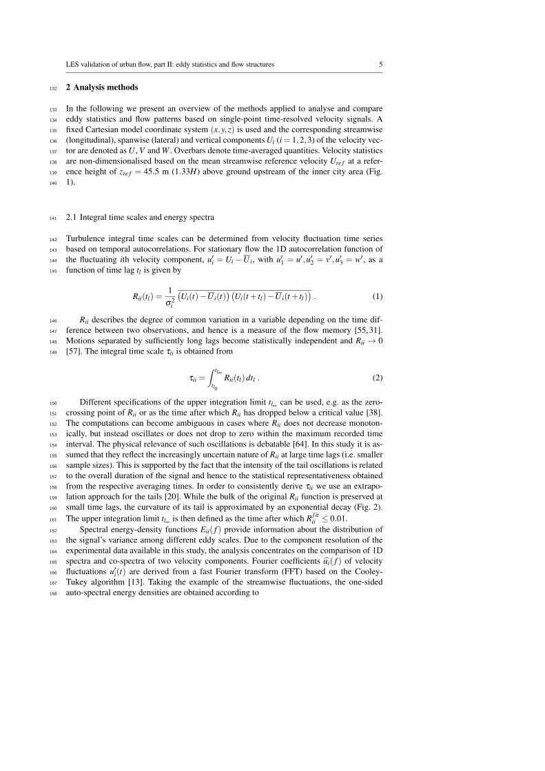
2 Analysis methods132

In the following we present an overview of the methods applied to analyse and compare133

eddy statistics and flow patterns based on single-point time-resolved velocity signals. A134

fixed Cartesian model coordinate system (x,y,z) is used and the corresponding streamwise135

(longitudinal), spanwise (lateral) and vertical components Ui (i = 1,2,3) of the velocity vec-136

tor are denoted as U , V and W . Overbars denote time-averaged quantities. Velocity statistics137

are non-dimensionalised based on the mean streamwise reference velocity Ure f at a refer-138

ence height of zre f = 45.5 m (1.33H) above ground upstream of the inner city area (Fig.139

1).140

2.1 Integral time scales and energy spectra141

Turbulence integral time scales can be determined from velocity fluctuation time series142

based on temporal autocorrelations. For stationary flow the 1D autocorrelation function of143

the fluctuating ith velocity component, u′i = Ui −U i, with u′1 = u′,u′2 = v′,u′3 = w′, as a144

function of time lag tl is given by145

Rii(tl) =1

σ2i

(Ui(t)−U i(t)

)(Ui(t + tl)−U i(t + tl)

). (1)

Rii describes the degree of common variation in a variable depending on the time dif-146

ference between two observations, and hence is a measure of the flow memory [55,31].147

Motions separated by sufficiently long lags become statistically independent and Rii → 0148

[57]. The integral time scale τii is obtained from149

τii =∫ tl∞

tl0

Rii(tl)dtl . (2)

Different specifications of the upper integration limit tl∞ can be used, e.g. as the zero-150

crossing point of Rii or as the time after which Rii has dropped below a critical value [38].151

The computations can become ambiguous in cases where Rii does not decrease monoton-152

ically, but instead oscillates or does not drop to zero within the maximum recorded time153

interval. The physical relevance of such oscillations is debatable [64]. In this study it is as-154

sumed that they reflect the increasingly uncertain nature of Rii at large time lags (i.e. smaller155

sample sizes). This is supported by the fact that the intensity of the tail oscillations is related156

to the overall duration of the signal and hence to the statistical representativeness obtained157

from the respective averaging times. In order to consistently derive τii we use an extrapo-158

lation approach for the tails [20]. While the bulk of the original Rii function is preserved at159

small time lags, the curvature of its tail is approximated by an exponential decay (Fig. 2).160

The upper integration limit tl∞ is then defined as the time after which R f itii ≤ 0.01.161

Spectral energy-density functions Eii( f ) provide information about the distribution of162

the signal’s variance among different eddy scales. Due to the component resolution of the163

experimental data available in this study, the analysis concentrates on the comparison of 1D164

spectra and co-spectra of two velocity components. Fourier coefficients ui( f ) of velocity165

fluctuations u′i(t) are derived from a fast Fourier transform (FFT) based on the Cooley-166

Tukey algorithm [13]. Taking the example of the streamwise fluctuations, the one-sided167

auto-spectral energy densities are obtained according to168

6 Denise Hertwig et al.

0 50 100 150 200 250

10−2

10−1

100

tl (s)

Rii(–)

0 50 100 150 200 2500

0.2

0.4

0.6

0.8

1

tl (s)

Rii(–)

RuuRvvRww

Fig. 2: Example of the fitting procedure applied to the Rii functions (here: wind tunnel data).Left: original curves together with the respective tail fit; right: concatenated signals usingthe original and fitted curves. The original curves are retained up to time lags for which Riihas dropped to a value between once or twice its e-folding time.

Euu( fk) =2

N fsu∗k uk =

2N2δ fs

|uk|2 , (3)

with the frequency index k = 0, . . . ,N/2, N is the number of samples in the signal,169

fs is the sampling frequency, δ fs = fk− fk−1 is the constant frequency increment and the170

asterisk denotes the complex conjugate [36]. In the same way energy density spectra Evv171

and Eww can be derived from spanwise and vertical velocity fluctuations, v′ and w′. For172

paired signals of u′ and w′ the co-spectrum Couw is computed according to Couw( fk) =173

Re{uk}Re{wk}+ Im{uk}Im{wk}.174

Earlier studies have shown that the unique roughness structure of urban surfaces leaves175

a distinct footprint in the spectra [45,46]. Inertial subrange behaviour in urban areas in terms176

of −5/3 slopes is comparable to flow over uniform roughness. However, based on a more177

stringent test for local isotropy, Rotach [45] found that urban flow is not truly isotropic in the178

inertial subrange at heights well within the roughness sublayer. The size of integral length179

scale eddies associated with the spectral peaks deviates from empirical reference relations180

for flow over homogeneous surfaces [25]. Roth [46] reported that within the UCL and in181

the vicinity of the canopy top, a shift towards higher frequencies is evident in the spectra182

of the horizontal velocities, while peaks in vertical velocity spectra are offset towards lower183

frequencies. The increase of the vertical eddy-length scale suggests that the vertical transport184

is dominated by wake turbulence that scales with the building dimensions.185

2.2 Conditional averaging186

A well-known representative of conditional resampling/averaging methods is the quadrant187

analysis [60,61,59], which can be applied, for example, to analyse the vertical turbulent188

momentum exchange u′w′. Instantaneous fluxes u′w′ are grouped into one of four quadrants189

based on the respective composition of the algebraic signs of u′ and w′. Following the nota-190

tion by Raupach [41], conditional averages of the momentum flux contributions from each191

of the four quadrants are obtained from192

LES validation of urban flow, part II: eddy statistics and flow structures 7

u′

w′

(u′w′)c

1 > 0(u′w′)c

2 < 0

(u′w′)c

3 > 0 (u′w′)c

4 < 0

ejection

sweep

outward interaction

inward interaction

Q1Q2

Q3 Q4

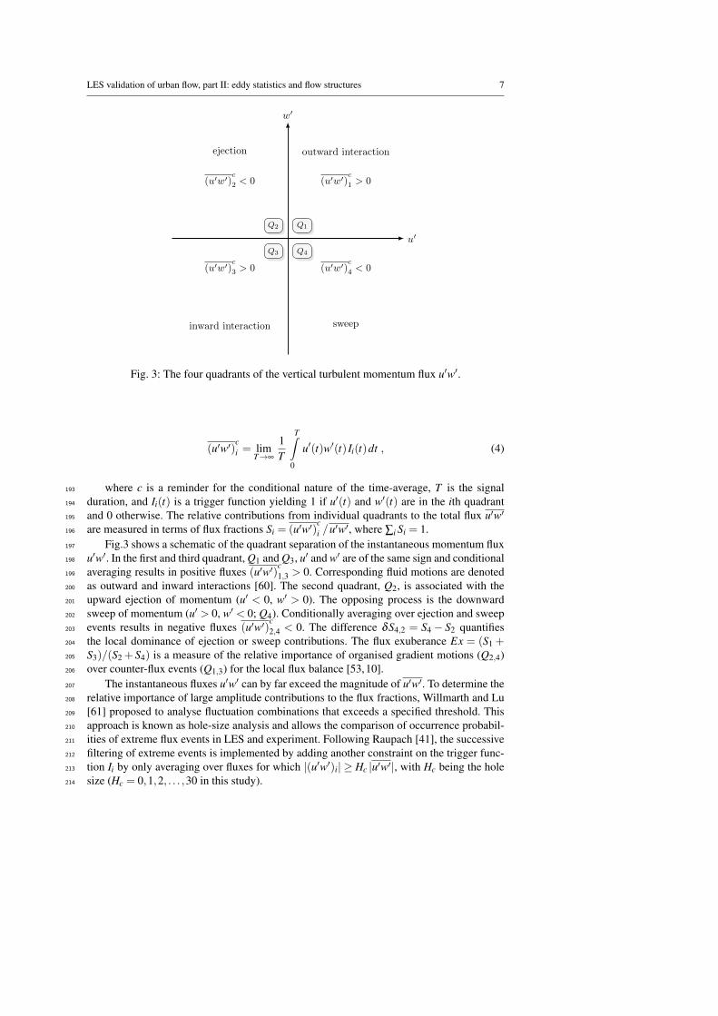
Fig. 3: The four quadrants of the vertical turbulent momentum flux u′w′.

(u′w′)ci = lim

T→∞

1T

T∫0

u′(t)w′(t) Ii(t)dt , (4)

where c is a reminder for the conditional nature of the time-average, T is the signal193

duration, and Ii(t) is a trigger function yielding 1 if u′(t) and w′(t) are in the ith quadrant194

and 0 otherwise. The relative contributions from individual quadrants to the total flux u′w′195

are measured in terms of flux fractions Si = (u′w′)ci /u′w′, where ∑i Si = 1.196

Fig.3 shows a schematic of the quadrant separation of the instantaneous momentum flux197

u′w′. In the first and third quadrant, Q1 and Q3, u′ and w′ are of the same sign and conditional198

averaging results in positive fluxes (u′w′)c1,3 > 0. Corresponding fluid motions are denoted199

as outward and inward interactions [60]. The second quadrant, Q2, is associated with the200

upward ejection of momentum (u′ < 0, w′ > 0). The opposing process is the downward201

sweep of momentum (u′ > 0, w′ < 0; Q4). Conditionally averaging over ejection and sweep202

events results in negative fluxes (u′w′)c2,4 < 0. The difference δS4,2 = S4 − S2 quantifies203

the local dominance of ejection or sweep contributions. The flux exuberance Ex = (S1 +204

S3)/(S2 + S4) is a measure of the relative importance of organised gradient motions (Q2,4)205

over counter-flux events (Q1,3) for the local flux balance [53,10].206

The instantaneous fluxes u′w′ can by far exceed the magnitude of u′w′. To determine the207

relative importance of large amplitude contributions to the flux fractions, Willmarth and Lu208

[61] proposed to analyse fluctuation combinations that exceeds a specified threshold. This209

approach is known as hole-size analysis and allows the comparison of occurrence probabil-210

ities of extreme flux events in LES and experiment. Following Raupach [41], the successive211

filtering of extreme events is implemented by adding another constraint on the trigger func-212

tion Ii by only averaging over fluxes for which |(u′w′)i| ≥ Hc |u′w′|, with Hc being the hole213

size (Hc = 0,1,2, . . . ,30 in this study).214

8 Denise Hertwig et al.

Within and above the UCL building-induced turbulence can induce strong turbulent mix-215

ing [46]. Through the analysis of the vertical momentum flux, the relative contributions of216

the upward transport of momentum deficit (ejection) and the downward transport of mo-217

mentum excess (sweep) in urban environments can be investigated [44]. At roof-level, the218

momentum exchange is often found to be dominated by sweeps. However, this prevalence219

vanishes at higher elevations. The dominance of sweeps within the UCL has been confirmed220

on the basis of field observations [37,10], showing that ejections are prevailing well above221

the canopy. Oikawa and Meng [37] described characteristic sweep and ejection patterns as-222

sociated with sudden fluid bursts and connected distinctive ramp structures in temperature223

signals with the passage of large-scale coherent eddies above the canopy. Based on condi-224

tional averages of ejection-sweep cycles within and above a street canyon, Feigenwinter and225

Vogt [18] showed that fluctuation levels were highest just above the canopy and decreased226

with increasing distance from the roofs. Christen et al. [10] described the role of coherent227

structures for turbulent exchange at the interface between canopy and roughness sublayer by228

associating ejection-sweep events with the advection and penetration of coherent structures229

from the roughness layer into the street canyon.230

2.3 Joint time-frequency analysis231

The wavelet transform is an important representative of joint time-frequency analysis meth-232

ods used for the time-localisation of a signal’s frequency content [34,22,23]. In effect, this233

approach adds the time dimension to the classic Fourier analysis by using wave functions of234

limited temporal support instead of non-local sinusoids. In the application to turbulent flows235

this means that the occurrence of eddy structures associated with certain frequencies can be236

studied in a time-dependent framework [32,15].237

Wavelets are oscillating, square-integrable, localised functions whose location and shape238

are manipulated during the transform process to unfold the time-frequency content of the239

signal [1]. The wavelet function ψs,n(t) = s−1/2ψ[(t− n)s−1] depends on two parameters.240

The translation parameter n shifts the wavelet along the time axis and the dilation parameter241

s > 0, also known as the scale of the wavelet, stretches (s > 1) or compresses (0 < s < 1)242

the function in order to retrieve low or high frequency information from the signal. This243

behaviour is illustrated in Fig. 4. The normalisation factor s−1/2 ensures finite energy content244

at all wavelet scales [26]. The continuous wavelet transform (CWT) of a time-dependent245

signal Φ(t) with zero mean and finite energy is given by246

Wn(s) =1√s

∫∞

−∞

Φ(t)ψ∗(

t−ns

)dt , (5)

where the asterisk denotes the complex conjugate. The wavelet coefficients Wn(s) con-247

tain time-frequency information about Φ(t). The time-frequency resolution of the CWT is248

variable. At large scales, the wavelet is less well localised in time than at small scales, while249

the frequency resolution is better than for contracted wavelets (Fig. 4). Like the Fourier250

transform, the CWT is reversible and the original signal can be reconstructed from the251

wavelet coefficients without information loss [36].252

For our analyses of velocity time series we use the complex Morlet wavelet defined as253

ψm(t) = Nψm exp(iω0t)exp(−t2/2). The central frequency ω0 is set to a value of 6 in this254

study, and Nψm = π−1/4 is a normalisation factor. We apply a discretised version of the CWT255

in spectral space [1,56]. For a discrete signal Φn = Φ(tn = nδ ts) sampled at time intervals256

LES validation of urban flow, part II: eddy statistics and flow structures 9

−6 −4 −2 0 2 4 6−1

−0.5

0

0.5

1

t (s)

s−1/2Re{ψm}(t /s)

s = 0.5 s = 1.0 s = 2.0

0 10 200

2

4

6

8

ω (Hz)

2πs|ψm|2(sω)

Fig. 4: Influence of the dilation parameter s on the shape of the Morlet wavelet in the time(left) and frequency domain (right), with the latter showing the wavelet’s energy spectrum.

10−3 10−2 10−1 100 101

10−3

10−2

10−1

100

fz/U (–)

fEuuσ−2

u,fEψ uuσ−2

u(–)

Eψ ?uu – CWT-based spectrum

E?uu – DFT-based spectrum

10−3 10−2 10−1 100 10110−4

10−3

10−2

10−1

100

fz/U (–)

fEuuσ−2

u,fEψ uuσ−2

u(–)

3

2

3

10

Fig. 5: Scaled auto-spectral energy densities of the streamwise velocity derived from thediscrete-time CWT using the Morlet wavelet (triangles) in comparison to the classic dis-crete Fourier transform (DFT) spectra (dots). Left: wind tunnel; right: LES. The spectracorrespond to a height of 45.5 m above the Elbe river (site BL04).

δ ts over a duration of T = Nδ ts, where N is the number of samples and n = 0, . . . ,N−1, the257

discrete-time CWT is given by258

Wn(s) =

√2πsδ ts

N−1

∑k=0

Φk ψ∗(sωk) exp(iωknδ ts) , (6)

where Φ and ψ are the Fourier transforms of the signal and the wavelet, respectively, k259

is a frequency index and ω = 2π f . The term before the sum is a normalisation factor that260

ensures that the wavelet function has unit energy at each scale. The Fourier transform of the261

Morlet wavelet is known analytically: ψm(ω) = NψmH (ω)exp(−(ω−ω0)2/2), where H262

is the Heaviside step function [56]. Eq. (6) is implemented by obtaining the inverse Fourier263

transform of the product of Φk and ψ∗(sωk) for all scales s at all translations n using an264

FFT algorithm [13]. Following [56], the series of scales s j is obtained as a fractional power265

of 2 according to s j = s0 2 j δ j, where s0 is the smallest scale and δ j is the spacing between266

scales. In this study we use s0 = δ ts and δ j = 1/8 following sensitivity tests.267

As the energy content of the signal is conserved in wavelet space, it is possible to obtain268

a global energy density spectrum based on Wn(s) similar to the spectrum available from the269

10 Denise Hertwig et al.

discrete Fourier transform [1]. Fig. 5 shows wind tunnel and LES energy-density spectra270

corresponding to a height of 45.5 m above the Elbe river derived from a discrete-time CWT271

using the complex Morlet wavelet in comparison to the classic Fourier spectra. Both, the272

−2/3 slope of the wind-tunnel inertial subrange as well as the much steeper slope of the LES273

spectrum (approximately −10/3 as a result of cutting off eddies smaller than the numerical274

grid) are very well resolved with the CWT. This fast energy decay is characteristic for LES275

spectra due to the spatial filtering and can only be adequately resolved with wavelets that276

have a high number of vanishing moments. With the Morlet wavelet using ω0 = 6 spectral277

slopes up to −7 can be reproduced [16].278

3 Eddy statistics279

In the following sections we present results of the validation test case based on detailed280

analyses of velocity time series. Results are only directly compared at heights for which the281

largest spatial offset between the LES and wind-tunnel data pairs was 0.25 m. This offset is282

well within the LDA’s spatial accuracy of 0.56 m full scale in z-direction when operated in283

U–V mode or in y-direction for U–W measurements (see part I for details).284

The validation results presented in the following paragraphs and in Sect. 4 represent285

only a subset of the analyses performed in the course of the validation study in order to286

focus on particular strengths and limitations of the model. The selection is representative of287

the overall agreement between experiment and LES.288

3.1 Integral time scales289

Integral time scales can be regarded as representative time scales of the dominant turbulence290

structures in the flow. Comparing their characteristics is therefore particularly important for291

eddy-resolving approaches such as LES.292

In the following, comparisons of τii and Rii are presented in full-scale dimensions. The293

full-scale time lags tl used to construct Rii(tl) were derived from their dimensionless equiv-294

alents t?l according to t?l = tl Ure f L−1re f , setting Ure f to 5 m s−1 and using reference lengths,295

Lre f , of 1 m for the laboratory flow and an equivalent of 350 m for the LES.296

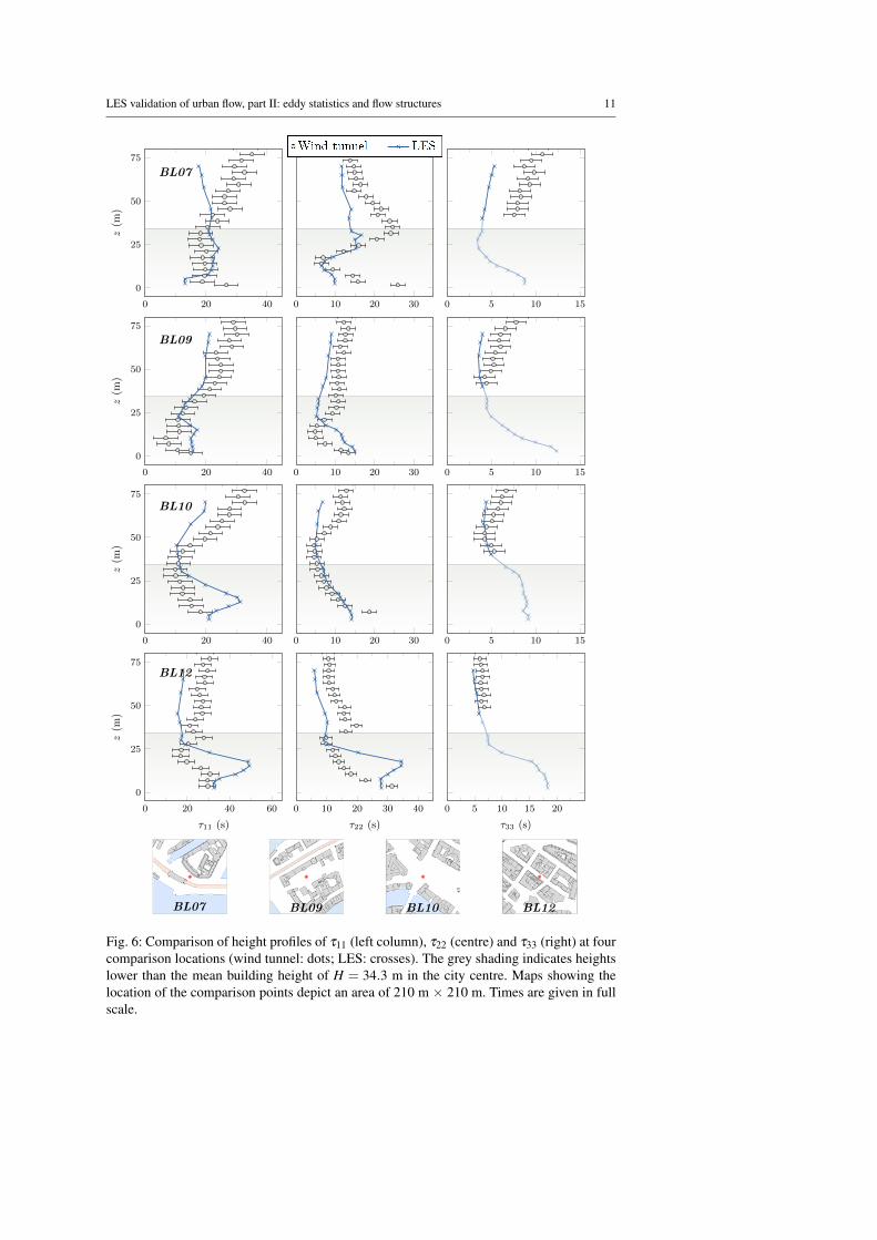
3.1.1 Vertical structure of τii297

Fig. 6 shows height profiles of Eulerian integral time scales for the three velocity compo-298

nents within the roughness sublayer up to approximately 2H at four of the BL comparison299

sites, for which measurements of all three velocity component are available from the refer-300

ence experiment. The statistical reproducibility of the experimental results was derived from301

repetition measurements, yielding full-scale maximum scatter of τ11±3.95 s, τ22±1.85 s,302

and τ33±1.17 s.303

Overall, the LES captures the qualitative height-dependence of the integral time scales304

at most of the sites. While there are some quantitative differences, the overall magnitude of305

turbulence time scales agrees with the experiment. A steady increase of τii is seen well above306

roof level, corresponding to an increase of eddy length scales in response to the gradual307

weakening of topology-induced flow effects. However, at site BL07 the decrease of the LES308

τ11 and low values of τ33 above H is opposite to the behaviour seen in the experiments.309

This site is located in the region where an internal boundary layer is starting to develop just310

LES validation of urban flow, part II: eddy statistics and flow structures 11

0 20 40

0

25

50

75

z(m

)

0 10 20 30 0 5 10 15

0 20 40

0

25

50

75

z(m

)

0 10 20 30 0 5 10 15

0 20 40

0

25

50

75

z(m

)

0 10 20 30 0 5 10 15

0 20 40 60

0

25

50

75

τ11 (s)

z(m

)

0 10 20 30 40

τ22 (s)

0 5 10 15 20

τ33 (s)

BL07

BL09

BL10

BL12

BL07 BL09 BL10 BL12

Fig. 6: Comparison of height profiles of τ11 (left column), τ22 (centre) and τ33 (right) at fourcomparison locations (wind tunnel: dots; LES: crosses). The grey shading indicates heightslower than the mean building height of H = 34.3 m in the city centre. Maps showing thelocation of the comparison points depict an area of 210 m × 210 m. Times are given in fullscale.

12 Denise Hertwig et al.

downstream of the river in response to the increased surface roughness of the high-density311

inner city. Here it seems that the upper layer flow field in the LES still is dominated by the312

artificial turbulence prescribed at the inflow plane of the simulation. Further downstream, as313

the flow adjusts to the new roughness underneath, the simulation above the UCL becomes314

more self-consistent, resulting in an increased level of agreement with the wind tunnel.315

The same is true for the height development of integral time scales τ33 associated with316

the vertical velocity from site BL07 to BL12. At elevations at which measurements are317

available, the τ33 of the LES are well within the experimental scatter at most heights in the318

downtown area (BL09–BL12). Within the UCL the LES predicts increased amplitudes of τ33319

(BL09, BL12), indicating enhanced memory effects associated with the vertical momentum320

exchange, for example associated with street-canyon ventilation at site BL12. Although di-321

rect validation of this simulation feature is not possible here due to the lack of experimental322

data points, the agreement of the magnitudes of τ11 and τ22 indicates that this is also true for323

τ33 for consistency reasons.324

The overall height structure of τii uniquely corresponds to the local building topology325

and thus changes strongly from site to site. For example, at sites BL10 (intersection) and326

BL12 (street canyon) strong vertical gradients in τ11 and τ22 can be observed within the327

UCL; a feature that is more pronounced in the LES. At all sites the wind-tunnel flow is328

characterised by long τ22 well within the UCL, indicating the existence of comparatively329

long-lived eddy structures. These features are also evident in the LES, although the peak330

heights and magnitudes differ at some of the locations, e.g. BL12.331

By comparing integral time scales at various sites, it could be shown that the LES re-332

sponds in a similar way to the local building morphology as the flow in the reference experi-333

ment. Here it is particularly important to analyse all three components of the velocity vector,334

as the urban flow field is highly three-dimensional and the LES should be able to reflect this335

complexity. This is crucial, for example, for the representation of horizontal and vertical336

mixing in turbulent dispersion processes. The results demonstrate the ability of the tested337

LES code to represent the time-scales of energy-dominating turbulence features realistically338

for the given application, even in a very complex geometry and with limitations imposed by339

the grid resolution.340

3.1.2 Structural information from Rii341

It is worthwhile to also investigate the shapes of the underlying temporal autocorrelation342

curves, Rii(tl) in order to derive further information about eddy structures.343

Two commonly observed features are shown in Fig. 7, depicting close-ups of LES and344

wind tunnel data at short time lags. Strikingly different curvatures of the LES and laboratory345

autocorrelations can be observed at tl ≤ 10 s. While the experimental curves are more-346

or-less straight lines, indicating a fast exponential decay (note the use of logarithmic y-347

axes), the eddies in the LES are slightly longer correlated over short times. This feature is348

characteristic of the spatially filtered nature of the LES, in which only the large eddies are349

directly resolved. As discussed by Townsend [57], in turbulent flows in which eddy sizes are350

in some way restricted the slope of the Rii functions is rather gentle at short time lags. If, on351

the other hand, a wide and continuous range of eddy structures is present in the flow, as is352

the case in the wind tunnel, the initial slope is significantly steeper.353

Another noticeable feature encountered at various locations in the urban domain is that354

some of the autocorrelation functions are composed of rapidly and slowly varying parts,355

a feature that is often more pronounced in the autocorrelations of the streamwise velocity356

fluctuations. The example of location RM10 (Fig. 7, left) shows that in both data sets the357

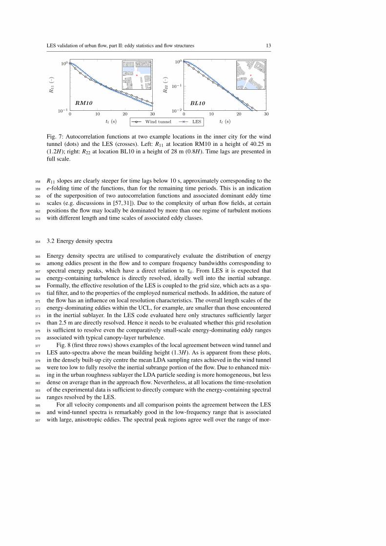
LES validation of urban flow, part II: eddy statistics and flow structures 13

RM10

0 10 20 3010−1

100

tl (s)

R11(–)

Wind tunnel LES

BL10

0 10 20 3010−2

10−1

100

tl (s)

R22(–)

Fig. 7: Autocorrelation functions at two example locations in the inner city for the windtunnel (dots) and the LES (crosses). Left: R11 at location RM10 in a height of 40.25 m(1.2H); right: R22 at location BL10 in a height of 28 m (0.8H). Time lags are presented infull scale.

R11 slopes are clearly steeper for time lags below 10 s, approximately corresponding to the358

e-folding time of the functions, than for the remaining time periods. This is an indication359

of the superposition of two autocorrelation functions and associated dominant eddy time360

scales (e.g. discussions in [57,31]). Due to the complexity of urban flow fields, at certain361

positions the flow may locally be dominated by more than one regime of turbulent motions362

with different length and time scales of associated eddy classes.363

3.2 Energy density spectra364

Energy density spectra are utilised to comparatively evaluate the distribution of energy365

among eddies present in the flow and to compare frequency bandwidths corresponding to366

spectral energy peaks, which have a direct relation to τii. From LES it is expected that367

energy-containing turbulence is directly resolved, ideally well into the inertial subrange.368

Formally, the effective resolution of the LES is coupled to the grid size, which acts as a spa-369

tial filter, and to the properties of the employed numerical methods. In addition, the nature of370

the flow has an influence on local resolution characteristics. The overall length scales of the371

energy-dominating eddies within the UCL, for example, are smaller than those encountered372

in the inertial sublayer. In the LES code evaluated here only structures sufficiently larger373

than 2.5 m are directly resolved. Hence it needs to be evaluated whether this grid resolution374

is sufficient to resolve even the comparatively small-scale energy-dominating eddy ranges375

associated with typical canopy-layer turbulence.376

Fig. 8 (first three rows) shows examples of the local agreement between wind tunnel and377

LES auto-spectra above the mean building height (1.3H). As is apparent from these plots,378

in the densely built-up city centre the mean LDA sampling rates achieved in the wind tunnel379

were too low to fully resolve the inertial subrange portion of the flow. Due to enhanced mix-380

ing in the urban roughness sublayer the LDA particle seeding is more homogeneous, but less381

dense on average than in the approach flow. Nevertheless, at all locations the time-resolution382

of the experimental data is sufficient to directly compare with the energy-containing spectral383

ranges resolved by the LES.384

For all velocity components and all comparison points the agreement between the LES385

and wind-tunnel spectra is remarkably good in the low-frequency range that is associated386

with large, anisotropic eddies. The spectral peak regions agree well over the range of mor-387

14 Denise Hertwig et al.

u′

BL0810−3

10−2

10−1

100

fEuuσ−2

u(-)

u′

BL09

u′

BL10

v′

BL0810−3

10−2

10−1

100

fEvvσ−2

v(-)

v′

BL09

v′

BL10

w′

BL0810−3

10−2

10−1

100

fEwwσ−2

w(-) w′

BL09

w′

BL10

(u′,w′)

BL08

10−3 10−2 10−1 100 10110−4

10−3

10−2

10−1

f z /U ( - )

−fCouw(σuσw)−

1 (u′,w′)

BL09

10−3 10−2 10−1 100 101

f z /U ( - )

(u′,w′)

BL10

10−3 10−2 10−1 100 101

f z /U ( - )

BL08 BL09 BL10

3

4

Fig. 8: Comparison of wind tunnel (dots) and LES (crosses) auto-spectral energy densitiesand co-spectra (bottom row) at three different locations in a height of 1.3H (45.5 m). Therespective velocity component analysed, i.e. u′, v′, w′ or (u′,w′), is indicated in the plots.The spectra are presented in a referenced framework based on the mean streamwise velocityU and the velocity variance σ2

i at height z. Maps show the location of the comparison sitesand their immediate surroundings.

LES validation of urban flow, part II: eddy statistics and flow structures 15

phologically rather different comparison sites. The fast roll-off of the numerical spectra at388

high frequencies is quite apparent, starting approximately after one decade into the inertial389

subrange. An interesting double-peak pattern in the v′-spectra is evident at site BL08 in390

both the laboratory and the simulation, implying a structural change in the flow. While the391

first peak corresponds to the peak frequency range characteristic for the approach flow (see392

BL04 spectra shown in Fig. 5), the second peak agrees well with the frequencies determined393

further downstream at the city locations (e.g. BL09, BL10). The increasing influence of the394

urban roughness on the flow field above the canopy is reflected in the fact that the size of395

the energy-containing eddies, measured by the frequency location of the energy peaks, is396

gradually decreasing. A similarly good agreement between both data sets is also seen below397

roof level at 0.5H (not shown).398

The bottom row of Fig. 8 shows co-spectra, Couw, of the streamwise and vertical velocity399

fluctuations. Compared to the auto-spectra the inertial-subrange slopes of the co-spectra are400

much steeper with a −4/3 power-law decay [63,25]. This indicates the importance of large401

eddies for the vertical turbulent momentum exchange u′w′ in the urban roughness sublayer.402

At all sites, the roll-off of the LES spectra is considerably faster, in agreement with the403

findings for the auto-spectra. Overall the flux-dominating frequency ranges in the LES agree404

very well with the wind tunnel. Even complex features like the double-peak pattern observed405

at location BL10 are remarkably well captured. In both data sets, the spectral maxima are406

shifting towards higher frequencies from the river site BL04 (not shown) to the downstream407

street canyon sites. This shows that the LES is captures the increasing influence of the urban408

environment on the flow and the importance of building-induced turbulence for vertical409

turbulent mixing.410

4 Flow structures411

The previous analyses are classic ways to infer information about the structure of turbulence,412

characteristic scales of dominant eddies and associated contributions to the variance of the413

flow field. In the next and final level of the validation study we now extend this analysis414

by investigating the dynamics of eddy structures by means of conditional resampling of the415

vertical momentum flux and joint time-frequency analysis.416

4.1 Quadrant analysis417

The comparison of the (u′,w′) co-spectra showed that the LES provides a realistic picture418

of the average flux contributions from different eddy classes. In the following, the structure419

of the instantaneous vertical turbulent momentum flux u′w′ is examined with quadrant anal-420

ysis. In a first step, the flux fractions defined in Eq. (4) are related to the associated joint421

probability density function (JPDF) of u′/Ure f and w′/Ure f . This approach provides a 2D422

extension of the analysis of velocity frequency distributions presented in part I.423

Fig. 9 shows comparisons of JPDFs at two example locations in a height of z = 1.3H:424

site BL07, located just downstream of the river upstream of the city core, and the downtown425

site BL10 at a complex intersection. Qualitatively, the overall shapes and extents of the426

joint PDFs in the (u′/Ure f ,w′/Ure f ) plane agree well. At both locations, the semi-major427

axes of the ellipses proceed through the Q2 and Q4 quadrants, indicating that the largest428

instantaneous flux amplitudes are associated with ejection and sweep episodes. At site BL07429

both joint PDFs are fairly symmetrical about the semi-major and semi-minor axes, with430

16 Denise Hertwig et al.

Q1Q2

Q3 Q4

Wind tunnel

−0.5 0 0.5

−0.5

0

0.5

u′/Uref ( - )

w′ /Uref(-)

Q1Q2

Q3 Q4

LES

−0.5 0 0.5

−0.5

0

0.5

u′/Uref ( - )w

′ /Uref(-)

0

0.5

1

1.5

2

2.5

3

3.5

4

4.5

ρ(u′?, w′?)

Q1Q2

Q3 Q4

Wind tunnel

−0.5 0 0.5

−0.5

0

0.5

u′/Uref ( - )

w′ /Uref(-)

Q1Q2

Q3 Q4

LES

−0.5 0 0.5

−0.5

0

0.5

u′/Uref ( - )

w′ /Uref(-)

0

0.5

1

1.5

2

2.5

ρ(u′?, w′?)

BL07

BL10

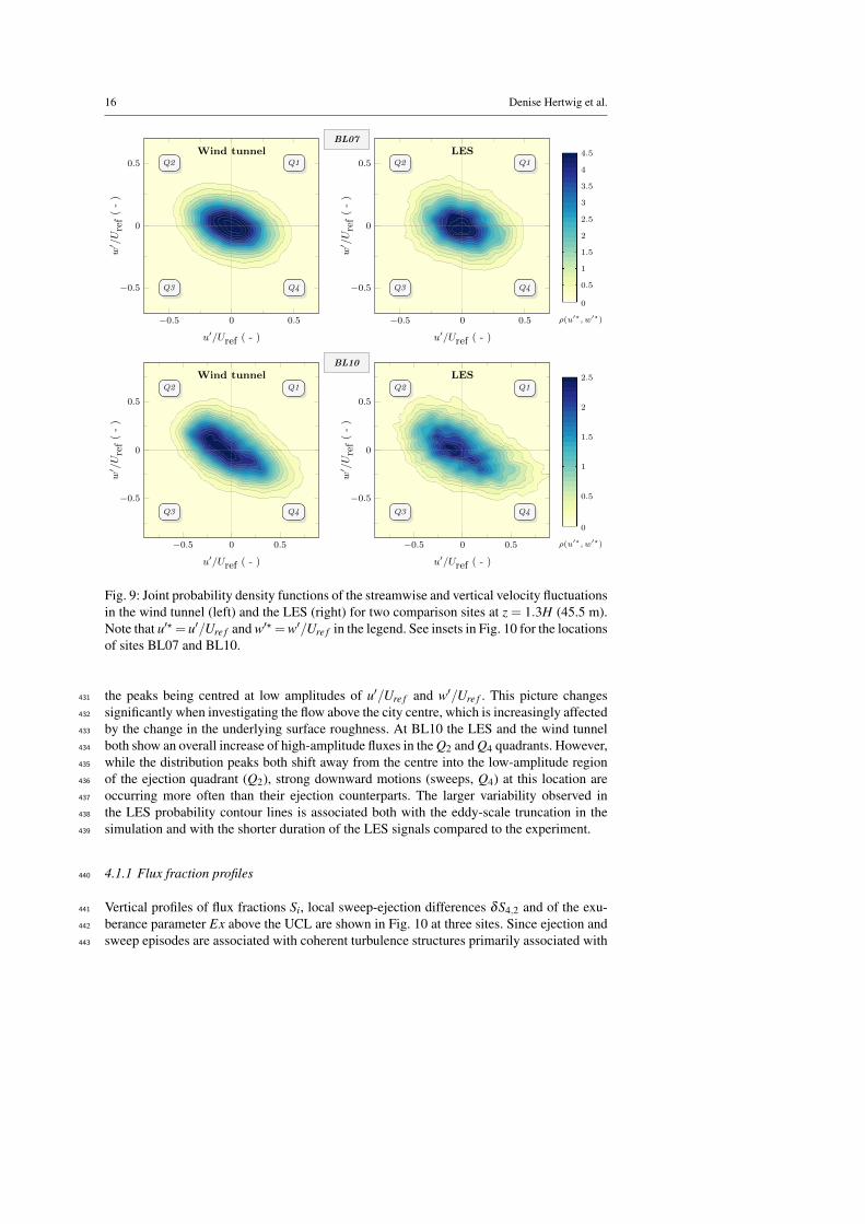
Fig. 9: Joint probability density functions of the streamwise and vertical velocity fluctuationsin the wind tunnel (left) and the LES (right) for two comparison sites at z = 1.3H (45.5 m).Note that u′? = u′/Ure f and w′? =w′/Ure f in the legend. See insets in Fig. 10 for the locationsof sites BL07 and BL10.

the peaks being centred at low amplitudes of u′/Ure f and w′/Ure f . This picture changes431

significantly when investigating the flow above the city centre, which is increasingly affected432

by the change in the underlying surface roughness. At BL10 the LES and the wind tunnel433

both show an overall increase of high-amplitude fluxes in the Q2 and Q4 quadrants. However,434

while the distribution peaks both shift away from the centre into the low-amplitude region435

of the ejection quadrant (Q2), strong downward motions (sweeps, Q4) at this location are436

occurring more often than their ejection counterparts. The larger variability observed in437

the LES probability contour lines is associated both with the eddy-scale truncation in the438

simulation and with the shorter duration of the LES signals compared to the experiment.439

4.1.1 Flux fraction profiles440

Vertical profiles of flux fractions Si, local sweep-ejection differences δS4,2 and of the exu-441

berance parameter Ex above the UCL are shown in Fig. 10 at three sites. Since ejection and442

sweep episodes are associated with coherent turbulence structures primarily associated with443

LES validation of urban flow, part II: eddy statistics and flow structures 17

−1 −0.5 0 0.5 130

40

50

60

70

80

z(m

)

S1 Wind tunnel S1 LES

S2 Wind tunnel S2 LES

S3 Wind tunnel S3 LES

S4 Wind tunnel S4 LES

−0.25 0 0.25

Wind tunnel LES

0 0.15 0.3 0.45 0.6

BL07

−1 −0.5 0 0.5 130

40

50

60

70

80

z(m

)

−0.25 0 0.25 0 0.15 0.3 0.45 0.6

BL10

−1 −0.5 0 0.5 130

40

50

60

70

80

Si (–)

z(m

)

−0.25 0 0.25

δS4,2 (–)

0 0.15 0.3 0.45 0.6

|Ex| (–)

BL11

Fig. 10: Comparison of vertical profiles of wind tunnel (open symbols) and LES (filled sym-bols) flux fractions Si (left), local differences between sweeps and ejections δS4,2 (centre)and magnitudes of the exuberance |Ex| (right) above the UCL. The grey shading indicatesheights lower than H.

large-scale eddies [10], turbulence-resolving time-dependent simulations should be able to444

resolve their general characteristics.445

At all sites ejection and sweep episodes clearly dominate the flow compared to counter-446

gradient fluxes, which is in agreement with other studies on surface-layer turbulence and447

flow characteristics within and above urban canopies, e.g. [41,44,37,17,10]. Overall, the448

LES captures the flux magnitudes associated with the respective quadrants. The qualitative449

18 Denise Hertwig et al.

response of the momentum exchange to the local roughness characteristics strongly resem-450

bles the laboratory observations. Slight differences in trends are found close to roof level,451

where the LES predicts a dominance of downward sweep motions (Q4) at all sites, while452

the laboratory flow shows a slight prevalence of ejections with the exception of location453

BL10. Higher up in the roughness sublayer, both the LES and the experiments show an454

ejection prevalence. While several of the studies cited above have documented a dominance455

of sweeps within and just above the canopy layer, this prevalence clearly is connected to the456

morphological characteristics of the analysis site and to the local flow structure. Especially457

in strongly heterogeneous canopies, like in this study, inferring general conclusions from458

local analyses is difficult.459

At the most upstream site BL07 the largest quantitative offsets between the wind tun-460

nel and LES Si profiles are observed, while qualitatively the height-dependent characteris-461

tics overall are well reproduced. Compared to locations further downstream here the LES462

and wind-tunnel flows are characterised by a larger proportion of counter-gradient fluxes at463

lower elevations. However, the exchange efficiency gradually increases with height as seen464

in the exuberance profiles |Ex(z)|. The smaller the exuberance magnitude, the more effi-465

cient the vertical turbulent momentum exchange through ejections and sweeps. The picture466

is different at the downtown sites BL10 and BL11, where the roughness-layer flow now is467

increasingly affected by three-dimensional building-induced mixing. The vertical momen-468

tum exchange is more efficient close to roof level (dominance of S2 + S4 over S1 + S3)469

and becomes less efficient at higher elevations. At the intersection site BL10 the qualitative470

and quantitative agreement is remarkably good. In the experiment and the LES the lowest471

comparison points are associated with a dominance of sweeps, while upward ejections are472

dominant further away from the canopy. The height profiles of δS4,2 exhibit strong gradients473

in a region between approximately 1.3H to 2H, reflecting an enhanced turbulent exchange474

between the flow field influenced by UCL turbulence and the upper-level flow. The largest475

magnitudes of Ex up to values of 0.6 are found at the lowest comparison heights at BL07.476

In contrast to that, at BL10 and BL11 the momentum exchange efficiency above the UCL477

is stronger: a change that is captured by the LES. The height ranges determined for the478

most efficient vertical momentum exchange are similar to those reported by Christen et al.479

[10] (1.0 < z/H < 1.25) from analyses of field measurements in a street canyon. In both480

the LES and the experiment, |Ex| converges to a nearly constant value of about 0.3 above481

2H, indicating a Gaussian distribution of the JPDFs in the (u′/Ure f ,w′/Ure f ) plane, again in482

agreement with field observations [10].483

4.1.2 Extreme events484

The above results show that the LES provides a realistic picture of time-dependent eddy485

dynamics in terms of instantaneous flux contributions from episodes of downward motions486

of air from the roughness sublayer towards the canopy and upward bursts of low-momentum487

fluid at different locations throughout the city. Such events often occur intermittently with488

large amplitudes of the instantaneous u′w′ fluxes as illustrated by the JPDFs (Fig. 9) and489

play an important role for canopy-layer ventilation or local detrainment and re-entrainment490

characteristics in street canyons. The occurrence of such strong ejection and sweep episodes491

can be related to the propagation of large-scale coherent eddy structures at the top of the492

canopy layer and to the contributions of building induced vortex shedding [27,11].493

In order to quantify and compare the relative importance of large amplitude contribu-494

tions to the flux fractions, a threshold parameter (hole size) Hc is introduced in a next step495

LES validation of urban flow, part II: eddy statistics and flow structures 19

Q2

0

0.2

0.4

0.6

0.8

1

|Si,H

c|

Q1

Q3

051015202530

0

0.2

0.4

0.6

0.8

1

Hc

|Si,H

c|

Q4

0 5 10 15 20 25 30

Hc

BL10

Q2

0

0.2

0.4

0.6

0.8

1

|Si,H

c|

Q1

Wind tunnel – 45.5m

LES – 45.25m

Wind tunnel – 70.0m

LES – 70.25m

Q3

051015202530

0

0.2

0.4

0.6

0.8

1

Hc|Si,H

c|

Q4

0 5 10 15 20 25 30

Hc

BL11

Fig. 11: The four flux fractions, |Si,Hc |, as a function of hole size, Hc, in the wind tunnel(dots) and LES (crosses) at two comparison sites in heights of 1.3H (45.5 m) and 2H (70 m).

as a further constraint on the conditional averaging (see Sect. 2.2). Low-amplitude contribu-496

tions to the total flux are successively filtered out such that the comparatively rare but strong497

remaining contributions to the momentum transport can be studied.498

Results of this analysis are shown in Fig. 11 for two heights within the roughness sub-499

layer: 1.3H (45.5 m) and 2H (70.25 m) at the city-centre sites BL10 and BL11. Depicted500

are flux fraction magnitudes, |Si,Hc |, as a function of hole size, Hc, for which we used a501

maximum value of 30 to cover the entire event space. The overall agreement of the hole-size502

dependent flux fractions computed from wind tunnel and the LES velocity time series is503

very high with regard to their qualitative and quantitative evolution. At both locations the504

dominance of ejection and sweep contributions (Q2, Q4) over the interaction quadrants (Q1,505

Q3) is preserved as the hole size is increased. Flux contributions from the counter-gradient506

Q1 and Q3 quadrants rapidly drop off as Hc is increased, showing that occurrences of strong507

flux episodes in these quadrants are very unlikely at the investigated sites. The only sig-508

nificant difference between the simulation and the experiment occurs at site BL10 in the509

Q2 quadrant at 70.25 m. Here the LES predicts larger contributions from high-amplitude510

fluxes than evident in the experiment. The corresponding JPDFs (Fig. 9) indicate that this511

is likely connected to the occurrence of slightly larger negative streamwise velocity fluctu-512

ations. In the second analysis height at the same location, however, a very good qualitative513

and quantitative agreement of the flux-fraction evolution in all four quadrants is found. Here514

the prevalence of ejection motions in the upper parts of the roughness sublayer is accom-515

panied by significant instantaneous turbulent flux episodes at large Hc. This is also the case516

at location BL11, where at both heights the behaviour of |Si,Hc | in the experiment and the517

simulation is quantitatively very similar.518

4.2 Wavelet analysis519

In the final level of the validation study, we analyse joint time-frequency information con-520

tained in the wavelet coefficients Wn(s) derived from velocity fluctuations as a time depen-521

dent extension of classic Fourier analysis. In order to study the turbulent flow with regard522

20 Denise Hertwig et al.

to the occurrence of certain eddy structures, the wavelet coefficients are analysed in terms523

of frequency distributions of the wind tunnel and LES data. For this purpose, the wavelet524

transform according to Eq. (6) is conducted using the Morlet wavelet (Fig. 4) for wavelet525

scales corresponding to frequencies in the energy-containing spectral range, resulting in526

frequency-dependent time series of wavelet coefficients.527

Fig. 12 shows frequency distributions of experimental and LES wavelet coefficients cor-528

responding to extraction frequencies of f ? = f z/U = 0.25, 0.75 and 1.0. These frequencies529

are all within the spectral peak range associated with eddies involved in turbulence produc-530

tion (see 1D spectra in Fig. 8). It was ensured that the fast roll-off of the LES spectra had not531

yet started at these frequencies, so that the information contained in the wavelet coefficients532

still corresponds to directly resolved scales. At these frequencies the local wavelet spectra533

are neither affected by aliasing at the highest frequencies nor by end effects arising from534

the analysis of signal portions at the beginning or end of the time series. The coefficients535

shown in Fig. 12 were obtained from streamwise velocity fluctuations in a height of 17.5 m536

(∼ 0.5H) at four sites corresponding to different urban settings. The time-dependent wavelet537

coefficients Wn( f ?) were normalised by the respective standard deviations of the coefficient538

time series, σW . Results are presented using semi-logarithmic axes since we are particularly539

interested in the tails of the distributions, which contain information about rare, intermittent540

events in the flow that leave a distinct footprint in the amplitudes of the wavelet coefficients.541

For a quantification of the level of agreement between the experimental and LES frequency542

distributions the kurtosis β of the samples are derived and displayed. In order to determine543

deviations from a normal distribution the corresponding Gaussian curves are shown.544

A common feature evident at all sites is that the wavelet coefficients most often exhibit545

small negative or positive amplitudes. The behaviour in the tails, on the other hand, is differ-546

ent at every site. This reflects differences in the local flow structure, but also shows a clear547

dependency on the frequency at which the coefficients are analysed. The smallest deviations548

from a normal distribution are found at the lowest frequency selected. For f ? = 0.75 and549

higher, the distributions feature heavier tails, reflecting an enhanced and intermittent activity550

in the flow associated with rare events and velocity bursts [16]. Deviations from the normal551

distribution are quantified by the respective values of β , which partially show significant552

offsets from the Gaussian reference (β = 3). In particular, the coefficient distributions tend553

to be more leptokurtic, i.e. they exhibit higher peaks and heavier tails than the normal distri-554

bution. This feature is seen in the experiment and the LES and similar frequency-dependent555

distribution characteristics can be determined at different comparison locations.556

At all sites the LES predictions are qualitatively and quantitatively in good agreement557

with the wind-tunnel experiment. At the intersection position BL10, for example, both558

the wind-tunnel and the LES wavelet coefficient distributions exhibit extended exponen-559

tial tails at the two highest extraction frequencies, recognisable as a linear decay in this560

semi-logarithmic representation. This feature illustrates the influence of the increased sur-561

face roughness on the spatial scales of dominant flow structures. Quadrant analysis showed562

that the location above the intersection is characterised by strong and intermittent vertical563

momentum exchange, dominated by sweep events. Similar tail behaviour is also detected564

at other comparison locations, notably at the river location BL04 ( f ? = 1.0). The kurtosis565

values indicate that the LES distributions have a tendency to be slightly more leptokurtic566

than the reference at f ? = 1.0, i.e. high amplitude oscillations in the wavelet coefficients567

are occurring more frequently than in the reference experiment. This could be a result of568

the proximity to the steep drop-off observed in the energy spectra. The increased level of569

intermittency could be an indication for the increased influence of the grid cut-off in the570

transition region between resolved and unresolved turbulence.571

LES validation of urban flow, part II: eddy statistics and flow structures 21

βWT = 3.6βLES = 3.0

−10 −5 0 5 1010−4

10−3

10−2

10−1

100

Rel.freq

uen

cy(–)

βWT = 4.1βLES = 4.4

−10 −5 0 5 10

βWT = 4.2βLES = 6.0

−10 −5 0 5 10

βWT = 3.5βLES = 3.3

−10 −5 0 5 1010−4

10−3

10−2

10−1

100

Rel.freq

uen

cy(–)

βWT = 4.2βLES = 4.5

−10 −5 0 5 10

βWT = 4.3βLES = 5.3

−10 −5 0 5 10

βWT = 3.4βLES = 3.3

−10 −5 0 5 1010−4

10−3

10−2

10−1

100

Rel.freq

uen

cy(–)

βWT = 4.6βLES = 4.7

−10 −5 0 5 10

βWT = 4.9βLES = 6.3

−10 −5 0 5 10

βWT = 3.0βLES = 2.9

−10 −5 0 5 1010−4

10−3

10−2

10−1

100

Wn(f∗)/σW (–)

Rel.freq

uen

cy(–)

βWT = 3.7βLES = 4.6

−10 −5 0 5 10

βWT = 3.9βLES = 4.7

−10 −5 0 5 10

Wn(f∗)/σW (–)

f∗ = 0.25 f∗ = 0.75 f∗ = 1.0

BL04

BL07

BL10

RM10

BL04 BL07 BL10 RM10

Fig. 12: Comparison of wind tunnel (dots) and LES (crosses) frequency distributions ofMorlet wavelet coefficients derived from streamwise velocity fluctuations at four locationsin a height of 0.5H (17.5 m). The distributions correspond to scaled frequencies of f ? =f z/U = 0.25 (left), 0.75 (centre) and 1.0 (right). The black lines show the correspondingGaussian distributions.

22 Denise Hertwig et al.

5 Discussion and conclusions572

5.1 Evaluation of the Hamburg test case573

The Hamburg validation test case showed that the quality of LES can be assessed in de-574

tail by not only focusing on comparisons of low-order statistics, but by taking into account575

the time-dependent nature of the problem. Following the multi-level validation concept pro-576

posed in part I we established that the tested LES code, FAST3D-CT, provides a realis-577

tic representation of mean flow and turbulence statistics in the urban roughness sublayer.578

This assessment was further substantiated by a direct comparison of time series in terms579

of frequency distributions, showing that the LES accurately reproduces complex geometry-580

induced flow patterns, e.g. flow-switching events reflected in bimodal velocity histograms.581

In part II presented here we have extended the analysis by examining the underlying flow582

structure in detail with regard to time-dependent flow statistics and flow features associated583

with energy and flux-dominating eddies that are directly resolved by the LES.584

5.1.1 Eddy scale and flow pattern analysis585

Compared to small-scale turbulence structures, energy and flux-dominating large-scale vor-586

tices occur less frequently. The representativity of associated statistical measures thus is587

strongly coupled to the duration of the signal, i.e. to the measurement or simulation time.588

Computational costs and computing time restrictions often result in the fact that there is589

a significant difference in LES signal lengths compared to the reference data, as was the590

case in our example study. While in this case the inherent uncertainty of low-order statis-591

tics obtained from the longer wind tunnel and shorter LES time series (Texp = 16.5 h and592

Tles = 6.5 h) is negligible compared to the experimental reproducibility, this may not be593

true for more sensitive parameters. An example is Si,Hc , which measures the relevance of594

extreme flux episodes associated with large, infrequently occurring eddies. The magnitude595

of this effect can for example be assessed based on the longer experimental data record.596

Repeating the hole-size analysis of Sect. 4.1.2 with a wind-tunnel time series that is shorter597

by a factor of Texp/Tles = 2.5 showed non-negligible differences in the flux fractions of the598

Q2,4 quadrants that are associated with coherent eddies. The larger the number of energy-599

dominating structures that have passed the sensor, the more robust are statistics associated600

with this eddy class. This has to be kept in mind when evaluating the agreement between601

LES and experiment.602

Eddy statistics Since reference data are still predominantly available in terms of single-point603

measurements, as was also the case in the test study, the focus should be on comparisons of604

dominant turbulence time scales and temporal autocorrelations to learn about the structure605

of the flow. In general, this can be extended into spatial correlation analyses given reference606

data of sufficient spatial resolution. For the model tested here, we found that the height de-607

pendence of integral time scales of the three velocity components overall is well reproduced608

in the simulation. Given the complexity of the canopy-layer flow field and the general sensi-609

tivity of measures based on correlations, this underlines the general suitability of the tested610

code for urban aerodynamics simulations.611

Analysing spectral energy densities allows the evaluation of contributions from eddies612

of different size to the local flow variance. With LES it is of particular interest to investigate613

up to what frequency range turbulence structures are directly resolved, which can be readily614

determined by the characteristic fast roll-off of the spectra as a result of the grid truncation.615

LES validation of urban flow, part II: eddy statistics and flow structures 23

In the Hamburg LES, the roll-off occurred in the transition region between the turbulence616

production range and the inertial subrange. Within the UCL, a scale decrease of the produc-617

tion range eddies is clearly reflected in the wind-tunnel spectra as a shift of the energy peaks618

towards higher frequencies. Given this eddy size reduction, the uniform grid resolution of619

2.5 m in combination with the implicit dissipation scheme causes the LES to be at the verge620

of being a “very large-eddy simulation” within the UCL. Despite this resolution limitation,621

at the majority of comparison sites the spectral shapes in the energy-dominating frequency622

range agree well with the experimental targets. This applies to frequency ranges associated623

with the spectral peak region and to the distribution of energy among the largest eddies in624

the flow, demonstrating that the LES accurately resolves turbulence that dominate the flow625

in terms of turbulence kinetic energy and turbulent mixing.626

Eddy structure and flow dynamics Within the atmospheric surface layer, turbulence is highly627

three-dimensional, particularly so within the urban canopy layer. Whether eddy-resolving628

simulation techniques are resolving the structure of turbulence in a realistic way can be629

analysed by means of structure identification methods, e.g. quadrant analysis, as done for the630

Hamburg test case. We showed that the efficiency of vertical momentum exchange, which is631

a quantity of interest for street-canyon ventilation or vertical detrainment, can be used as a632

quality control measure for the simulation. In the test case, for example, the LES produced633

momentum flux characteristics that are in agreement with the reference case regarding the634

local dominance of upward or downward motions associated with coherent eddy structures635

(gradient-type motions). Carrying out these comparisons at structurally different flow lo-636

cations allows the study of changes in the characteristics of flux events in response to the637

underlying roughness. By introducing a hole-size constraint to the conditional re-sampling638

process, the occurrence of flux contributions linked to infrequent, high-amplitude events639

in the flow was evaluated. The good agreement of the Hc-dependent flux fractions shows640

that the LES realistically represents the local dominance of downward sweeps of high-641

momentum fluid towards the UCL and upward ejections of low-momentum fluid into the642

upper parts of the roughness sublayer.643

Extending the classic Fourier analysis, the time-dependent flow structure can be com-644

pared in a joint time-frequency framework. Scale-dependent analyses of the turbulent flow645

field based on wavelet transform methods offer strong potential here, and in the Hamburg646

test case revealed a structural agreement of the time-dependent experimental and LES flows.647

The comparison of frequency distributions of wavelet coefficients extracted at energetically648

dominant frequencies reveal occurrence characteristics of rare but energetically significant649

turbulence episodes. Depending on the extraction frequency and the comparison location,650

the wavelet coefficient PDFs can feature heavy tails, which is an indication for an increased651

level of intermittency in the flow. By comparing the kurtosis values associated with the dis-652

tributions the level of agreement can be quantified.653

5.1.2 Model accuracy654

Applying the proposed validation strategy showed that FAST3D-CT provides realistic and655

reliable information about urban turbulence with regard to geometry-induced mean and in-656

stantaneous flow features. Despite the overall strong performance of FAST3D-CT some657

systematic discrepancies were identified. In part I we discussed how the grid resolution of658

2.5 m in combination with the computational representation of buildings by simple grid659

masking negatively affected the comparison, particularly in narrow street canyons. Spectral660

analyses performed in part II revealed how the grid resolution also affected the resolution661

24 Denise Hertwig et al.

potential of flow structures in the implicit LES. Although a grid-resolution of 2.5 m should662

make it possible to resolve at least one frequency decade of inertial subrange turbulence,663

the FCT-scheme handling the numerical dissipation in the model in its current configuration664

seemed to contribute to an enhanced energy loss, identifiable in the turbulence spectra. In665

general it can be expected that this also has an effect on mean flow and turbulence statistics,666

adding to the other sources of discrepancies identified before. Within the UCL, FAST3D-CT667

in this study only fully resolved eddies in the production range, which is characteristic for668

a very large-eddy simulation. The grid resolution also affected the overall comparability of669

the data due to spatial offsets between comparison locations in the experiment and the LES.670

Seemingly marginal height differences in the order of 0.25 m can have a significant influence671

on the results in regions of strong flow gradients. The same is true for spatial offsets in the672

(x,y) plane in strongly heterogeneous flow situations or near building walls. Re-running the673

Hamburg case with a more detailed representation of buildings, e.g. based on unstructured674

meshes or immersed boundary methods, would certainly lead to a better understanding of675

some of the discrepancies determined here. It can be expected that there will be improve-676

ments particularly at comparison points located in narrow streets. The same can be expected677

of refinements of the grid resolution in connection with the FCT-scheme, and improvements678

of the inflow modelling. In order to disentangle these overlapping sources of inaccuracy and679

to determine the effects of a better reproduction of low-frequency inertial range eddies, the680

resolution would need to be increased to 1 m or below. However, these improvements in-681

evitably lead to higher computational costs. For example, doubling the grid resolution will682

result in a sixteen-fold increase in run time. Alternatively, the simulation could be re-run in683

a much smaller domain, making the increase in grid resolution affordable, while possibly684

also being able to explore more accurate buildings representation techniques.685

5.2 Conclusions and outlook686

The work presented here was motivated by the lack of proportion between the increasing687

use of eddy-resolving CFD methods like LES for micro-meteorological and environmental688

fluid mechanics applications and the level of scrutiny that is commonly applied to vali-689

date the simulation results. Based on the example of highly complex urban boundary-layer690

flow we showed that through a rigorous validation against qualified reference data based691

on model-specific tests, the suitability of time-dependent, turbulence-resolving simulations692

for their intended use can be documented, and the bounds of uncertainty in the results can693

be quantified. With well-established signal analysis methods and by means of suitable and694

quality-controlled reference data, a high level of detail can be incorporated into the vali-695

dation of LES. The information gained by far exceeds what can be learned based on the696

traditional approach of comparing mean flow and turbulence statistics. By applying the se-697

quence of analysis methods to the Hamburg flow simulation we were able to validate, for698

example, the representation of699

– Velocity fluctuations in response to local flow structure700

– Time scales associated with dominant turbulent eddies701

– Distribution of energy among flow structures of different size702

– Turbulent exchange efficiency associated with different eddy structures703

– Contribution of extreme events to local turbulent exchange characteristics704

– Flow intermittency captured in time-dependent energy spectra.705

While the validation method was tested based on the specific case of urban turbulence,706

it can also be applied to validate other types of eddy-resolving boundary-layer simulations,707

LES validation of urban flow, part II: eddy statistics and flow structures 25

for example flow within and above plant canopies or above a uniform roughness (e.g. only708

prescribed through the roughness length). Similar validation concepts based on time-series709

analyses can also be applied to validate simulations of scalar dispersion or heat exchange.710

The methods can also be applied to other types of turbulence-resolving simulations to study711

local-scale problems like detached eddy simulation or direct numerical simulations, but also712

to high-resolution meteorological models (O(10− 100 m)) applied to study problems in713

which length-scales of energy-dominating eddies scale with the boundary-layer depth.714

The study showed that experiments in boundary-layer wind tunnels with full control over715

mean inflow and boundary conditions, flexibility in the geometric design of the test case and716

measurement repeatability offer great potential for model validation. However, wind-tunnel717

experiments themselves are models with strong geometric and physical abstractions. The718

potential, for example, to realistically model effects like differential heating on surfaces, an-719

thropogenic heating, evapo-transpiration from vegetation, strong convection or stable strat-720

ification in wind tunnels is limited. Therefore, ideally laboratory studies are accompanied721

by full-scale field experiments and vice versa. While only the latter can capture the full722

complexity of natural atmospheric flows, the former allows the systematic study of relevant723

processes in isolation. Urban studies for which field and wind-tunnel data are available and724

in the past were used for comprehensive model validation include for example the DAPPLE725

experiment in central London [62], the MUST experiment in the Utahn desert [5,47] or the726

Joint Urban 2003 campaign in Oklahoma City [24].727

LES is increasingly applied to real-life problems of practical concern and quality as-728

surance is becoming more and more crucial. Community-wide activities are now needed729

in order to streamline model validation efforts. Micro-meteorology and wind engineering730

communities have demonstrated before that multi-national, multi-institutional activities for731

the harmonisation of validation approaches for flow in urban environments are feasible. The732

COST Actions 732 [7,48,21] and ES1006 [58] are encouraging examples of how exchange733

between experimentalists and modellers can result in broadly accepted model quality stan-734

dards, best-practice simulation protocols and validation guidelines for flow and dispersion735

models applied to problems on the urban micro-scale. Similar activities need to be pursued736

for LES, involving model developers and users as well as field and laboratory experimental-737

ists. For micro-meteorological and environmental fluid mechanics applications in the near-738

surface boundary layer, the joint formulation of validation guidelines need to stress the role739

of advanced turbulence analysis methods and flow structure recognition techniques, and the740

need for standards regarding quality and quantity requirements for reference data.741

Acknowledgements The numerical simulations with the LES code FAST3D-CT were carried out at the742

Laboratories for Computational Physics and Fluid Dynamics of the U.S. Naval Research Laboratory in Wash-743

ington D.C., USA. The authors wish to express their thanks to Jay Boris, Mi-Young Obenschain and other744

collaborators there. Further thanks is given to colleagues at the Environmental Wind Tunnel Laboratory at the745

University of Hamburg. Financial funding by the German Federal Office of Civil Protection and Disaster As-746

sistance as well as by the Ministry of the Interior of the City of Hamburg within the “Hamburg Pilot Project” is747

gratefully acknowledged (BBK research contract no. BBK III.1-413-10-364). Parts of the wind-tunnel model748

construction were financially supported by the KlimaCampus at the University of Hamburg.749

References750

1. Addison, P.S.: The illustrated wavelet transform handbook: Introductory theory and applications in sci-751

ence, engineering, medicine and finance. Institute of Physics Publishing, London (2002)752

2. Adrian, R.J.: Hairpin vortex organization in wall turbulence. Phys Fluids 19, 041,301 (2007)753

26 Denise Hertwig et al.

3. Basu, S., Vinuesa, J.F., Swift, A.: Dynamic les modeling of a diurnal cycle. J Appl Meteorol Climatol754

47, 1156–1174 (2008)755

4. Beare, R.J., Macvean, M.K., Holtslag, A.A.M., Cuxart, J., Esau, I., Golaz, J.C., Jimenez, M.A., Khairout-756

dinov, M., Kosovic, B., Lund, D.L.T.S., Lundquist, J.K., McCabe, A., Moene, A.F., Noh, Y., Raasch, S.,757

Sullivan, P.: An intercomparison of large-eddy simulations of the stable boundary layer. Bound-Lay758

Meteorol 118, 247–272 (2006)759

5. Biltoft, C.A.: Customer report for MOck Urban Setting Test (MUST). Tech. Rep. WDTC-FR-01-121,760

West Desert Test Center, U.S. Army Dugway Proving Ground, Dugway (UT), USA (2001)761

6. Boppana, V.B.L., Xie, Z.T., Castro, I.P.: Large-eddy simulation of dispersion from surface sources in762

arrays of obstacles. Bound-Lay Meteorol 135, 433–454 (2010)763

7. Britter, R., Schatzmann, M. (eds.): Model evaluation guidance and protocol document. COST Action764

732. University of Hamburg, Germany (2007b)765

8. Chlond, A., Bohringer, O., Auerswald, T., Muller, F.: The effect of soil moisture and atmospheric condi-766

tions on the development of shallow cumulus convection: A coupled large-eddy simulation land surface767

model study. Meteorol Z 23(5), 491–510 (2014)768

9. Chow, F.K., Weigel, A.P., Street, R.L., Rotach, M.W., Xue, M.: High-resolution large-eddy simulations769

of flow in a steep alpine valley. Part I: Methodology, verification, and sensitivity experiments. J Appl770

Meteorol Climatol 45, 63–86 (2006)771

10. Christen, A., van Gorsel, E., Vogt, R.: Coherent structures in urban roughness sublayer turbulence. Int J772

Climatol 27, 1955–1968 (2007)773

11. Coceal, O., Dobre, A., Thomas, T.G.: Unsteady dynamics and organized structures from DNS over an774

idealized building canopy. Int J Climatol 27, 1943–1953 (2007)775

12. Conzemius, R., Fedorovich, E.: Bulk models of the sheared convective boundary layer: Evaluation776

through large eddy simulations. J Atmos Sci 64, 786–807 (2007)777

13. Cooley, J.W., Tukey, J.W.: An algorithm for the machine calculation of complex Fourier series. Math778

Comput 19, 297–301 (1965)779

14. Deardorff, J.W.: A numerical study of three-dimensional turbulent channel flow at large Reynolds num-780

bers. J Fluid Mech 41, 453–480 (1970)781

15. Farge, M.: Wavelet transforms and their application to turbulence. Annu Rev Fluid Mech 24, 395–457782

(1992)783

16. Farge, M., Schneider, K., Pannekoucke, O., Nguyen van yen, R.: Multiscale representations. In: H.J.S.784

Fernando (ed.) Handbook of Environmental Fluid Dynamics, vol. II: Systems, Pollution, Modeling, and785

Measurements. CRC Press (2012)786

17. Feddersen, B.: Wind tunnel modelling of turbulence and dispersion above tall and highly dense urban787

roughness. Ph.D. thesis, Swiss Federal Institute of Technology (2005). Diss. ETH No. 15934788

18. Feigenwinter, C., Vogt, R.: Detection and analysis of coherent structures in urban turbulence. Theor789

Appl Climatol 81, 219–230 (2005)790

19. Finnigan, J.J.: Turbulence in plant canopies. Annu Rev Fluid Mech 32, 519–571 (2000)791

20. Fischer, R.: Entwicklung eines problemorientierten Software-Pakets zur automatisierten Aufbereitung,792

Analyse und Dokumentation von im Windkanal produzierten Daten zur LES-Validierung. Ph.D. thesis,793

University of Hamburg (2011). In German794

21. Franke, J., Hellsten, A., Schlunzen, K.H., Carissimo, B.: The COST 732 Best Practice Guideline for795

CFD simulation of flows in the urban environment: a summary. Int J Environ Pollut 44, 419–427 (2011)796

22. Grossmann, A., Morlet, J.: Decomposition of Hardy functions into square integrable wavelets of constant797

shape. SIAM J Math Anal 15, 723–736 (1984)798

23. Grossmann, A., Morlet, J., Paul, T.: Transforms associated to square integrable group representations I:799

General results. J Math Anal 26, 2473–2479 (1985)800

24. Harms, F., Leitl, B., Schatzmann, M., Patnaik, G.: Validating LES-based flow and dispersion models. J801

Wind Eng Ind Aerod 99, 289–295 (2011)802

25. Kaimal, J.C., Wyngaard, J.C., Izumi, Y., Cote, O.R.: Spectral characteristics of surface-layer turbulence.803

Q J Roy Meteor Soc 98, 563–589 (1972)804

26. Kaiser, G.: A Friendly Guide to Wavelets, first edn. Birkhauser Boston (1994)805

27. Kanda, M., Moriwaki, R., Kasamatsu, F.: Large-eddy simulation of turbulent organized structures within806

and above explicitly resolved cube arrays. Bound-Lay Meteorol 112, 343–368 (2004)807

28. Letzel, M.O.: Urban large-eddy simulation (LES), Advanced computational fluid dynamics for urban808

climatic maps. In: E. Ng, C. Ren (eds.) The Urban Climatic Map: A Methodology for Sustainable Urban809

Planning, chap. 32, pp. 421–428. Routledge, New York (2015)810

29. Letzel, M.O., Raasch, S.: Large eddy simulation of thermally induced oscillations in the convective811

boundary layer. J Atmos Sci 60, 2328–2341 (2003)812

30. Lilly, D.K.: The representation of small-scale turbulence in numerical simulation experiments. In: H.H.813

Goldstine (ed.) Proceedings of the IBM Scientific Computing Symposium on Environmental Sciences,814

pp. 195–210. Yorktown Height, New York (1967)815

LES validation of urban flow, part II: eddy statistics and flow structures 27

31. Lumley, J.L., Panofsky, H.A.: The Structure of Atmospheric Turbulence. Interscience Publishers, New816

York (1964)817

32. Meneveau, C.: Analysis of turbulence in the orthonormal wavelet representation. J Fluid Mech 232,818

469–520 (1991)819

33. Michioka, T., Chow, F.K.: High-resolution large-eddy simulation of scalar transport in atmospheric820

boundary layer flow over complex terrain. J Appl Meteorol Climatol 47, 3150–3169 (2008)821

34. Morlet, J.: Sampling theory and wave propagation. In: Proceedings of the 51st Annual International822

Meeting of the Society of Exploration Geophysicists. Los Angeles (CA), USA (1981)823

35. Nieuwstadt, F.T.M., Mason, P.J., Moeng, C.H., Schumann, U.: Large-eddy simulation of the convective824

boundary layer: A comparison of four computer codes. In: F. Durst, B.E. Launder, R. Friedrich, F.W.825

Schmidt (eds.) Turbulent Shear Flows 8, pp. 343–367. Springer (1993)826

36. Nobach, H., Tropea, C., Cordier, L., Bonnet, J.P., Delville, J., Lewalle, J., Farge, M., Schneider, K.,827

Adrian, R.J.: Review of some fundamentals of data processing. In: C. Tropea, A.L. Yarin, J.F. Foss828

(eds.) Springer Handbook of Experimental Fluid Mechanics, Part D: Analysis and Post-Processing of829

Data. Springer (2007)830

37. Oikawa, S., Meng, Y.: Turbulence characteristics and organized motion in a suburban roughness sublayer.831

Bound-Lay Meteorol 74, 289–312 (1995)832

38. O’Neill, P.L., Nicolaides, D., Honnery, D., Soria, J.: Autocorrelation functions and the determination833

of integral length with reference to experimental and numerical data. In: Proceedings of the 15th Aus-834

tralasian Fluid Mechanics Conference. The University of Sydney, Sydney, Australia (2004)835

39. Patnaik, G., Boris, J.P., Grinstein, F.F., Iselin, J.P., Hertwig, D.: Large scale urban simulations with836

FCT. In: D. Kuzmin, R. Lohner, S. Turek (eds.) Flux-Corrected Transport: Principles, Algorithms, and837

Applications, Scientific Computing, second edn., pp. 91–117. Springer (2012)838

40. Patnaik, G., Grinstein, F.F., Boris, J.P., Young, T.R., Parmhed, O.: Large-scale urban simulations. In: F.F.839

Grinstein, L.G. Margolin, W.J. Rider (eds.) Implicit Large Eddy Simulation: Computing Turbulent Fluid840

Dynamics. Cambridge University Press (2007)841

41. Raupach, M.R.: Conditional statistics of Reynolds stress in rough-wall and smooth-wall turbulent bound-842

ary layers. J Fluid Mech 108, 363–382 (1981)843

42. Raupach, M.R., Thom, A.S.: Turbulence in and above plant canopies. Ann Rev Fluid Mech 13, 97–129844

(1981)845

43. Robinson, S.K.: Coherent motions in the turbulent boundary layer. Annu Rev Fluid Mech 23, 601–639846

(1991)847

44. Rotach, M.W.: Turbulence close to a rough urban surface - Part I: Reynolds stresses. Bound-Lay Mete-848

orol 65, 1–28 (1993)849

45. Rotach, M.W.: Profiles of turbulence statistics in and above an urban street canyon. Atmos Environ 29,850

1473–1486 (1995)851

46. Roth, M.: Review of atmospheric turbulence over cities. Q J Roy Meteor Soc 126, 941–990 (2000)852

47. Sabatino, S.D., Buccolieri, R., Olesen, H.R., Ketzel, M., Berkowicz, R., Franke, J., Schatzmann, M.,853

Schlunzen, K., Leitl, B., Britter, R., Borrego, C., Costa, A., Castelli, S., Reisin, T., Hellsten, A., Saloranta,854

J., Moussiopoulos, N., Barmpas, F., Brzozowski, K., Goricsan, I., Balczo, M., Bartzis, J., Efthimiou, G.,855

Santiago, J., Martilli, A., Piringer, M., Baumann-Stanzer, K., Hirtl, M., Baklanov, A., Nuterman, R.,856

Starchenko, A.: COST 732 in practice: the MUST model evaluation exercise. Int J Environ Pollut 44,857

403–418 (2011)858

48. Schatzmann, M., Britter, R.: Quality assurance and improvement of micro-scale meteorological models.859

Int J Environ Pollut 44, 139–146 (2011)860

49. Schlegel, F., Stiller, J., Bienert, A., Maas, H.G., Queck, R., Bernhofer, C.: Large-eddy simulation of861

inhomogeneous canopy flows using high resolution terrestrial laser scanning data. J Fluid Mech 142,862

223–243 (2012)863

50. Schumann, U.: Subgrid scale model for finite difference simulations of turbulent flows in plane channels864

and annuli. J Comput Phys 18, 376–404 (1975)865

51. Seifert, A., Heus, T., Pincus, R., Stevens, B.: Large-eddy simulation of the transient and near-equilibrium866

behavior of precipitating shallow convection. J Adv Model Earth Sy 7, 1918–1937 (2015)867

52. Shaw, R.H., Schumann, U.: Large-eddy simulation of turbulent flow above and within a forest. Bound-868

Lay Meteorol 61(1), 47–64 (1992)869

53. Shaw, R.H., Tavangar, J., Ward, D.P.: Structure of Reynolds stress in a canopy. J Clim Appl Meteorol870

22, 1922–1931 (1983)871

54. Smagorinsky, J.: General circulation experiments with the primitive equations: I. The basic experiment.872

Mon Weather Rev 91, 99–164 (1963)873

55. Stull, R.B.: An Introduction to Boundary Layer Meteorology. Kluwer Academic Publishers, Dordrecht874

(1988)875

56. Torrence, C., Compo, G.P.: A practical guide to wavelet analysis. B Am Meteorol Soc 79, 61–78 (1998)876

28 Denise Hertwig et al.

57. Townsend, A.A.: The Structure of Turbulent Shear Flow. Cambridge University Press, Cambridge (1956)877

58. Trini Castelli, S., Baumann-Stanzer, K., Leitl, B., Milliez, C.M., Berbekar, E., Rakai, A., Fuka, V., Hell-878

sten, A., Petrov, A., Efthimiou, G., Andronopoulos, S., Tinarelli, G., Tavares, R., Armand, P., Gariazzo,879

C., Jurcakova, K., Gasparac, G.: Evaluation of local-scale models for accidental releases in built envi-880

ronments: Results of the modelling exercises in cost action es1006. In: G.D. Steyn, N. Chaumerliac881

(eds.) Air Pollution Modeling and its Application XXIV, pp. 497–502. Springer International Publishing882

(2016)883

59. Wallace, J.M.: Quadrant analysis in turbulence research: history and evolution. Annu Rev Fluid Mech884

48, 131–158 (2016)885

60. Wallace, J.M., Eckelmann, H., Brodkey, R.: The wall region in turbulent shear flow. J Fluid Mech 53,886

39–48 (1972)887

61. Willmarth, W.W., Lu, S.S.: Structure of the Reynolds stress near the wall. J Fluid Mech 55, 65–92 (1972)888

62. Wood, C.R., Barlow, J.F., Belcher, S.E., Dobre, A., Arnold, S.J., Balogun, A.A., Lingard, J.J.N., Smal-889

ley, R.J., Tate, J.E., Tomlin, A.S., Britter, R.E., Cheng, H., Martin, D., Petersson, F.K., Shallcross, D.E.,890

White, I.R., Neophytou, M.K., Robins, A.G.: Dispersion experiments in central London: The 2007 DAP-891

PLE project. B Am Meteorol Soc 90, 955–969 (2009)892

63. Wyngaard, J.C., Cote, O.R.: Cospectral similarity in the atmospheric surface layer. Q J Roy Meteorol893

Soc 98, 590–603 (1972)894

64. Yaglom, A.M.: Correlation Theory of Stationary and Related Random Functions I: Basic Results.895

Springer (1987)896

65. Yue, W., Parlange, M.B., Meneveau, C., Zhu, W., van Hout, R., Katz, J.: Large-eddy simulation of plant897

canopy flows using plant-scale representation. Bound-Lay Meteorol 124, 183–203 (2007)898