predictive les modeling and validation of high-pressure turbulent
TRANSCRIPT
Modeling Flashback Propensity using LES and Experiments
Venkat RamanUniversity of Michigan
Noel ClemensThe University of Texas at Austin
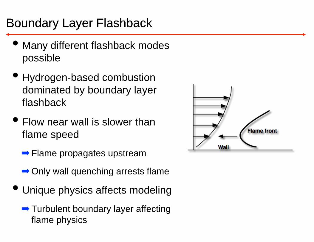
Boundary Layer FlashbackBoundary Layer Flashback
• Many different flashback modes possible
• Hydrogen-based combustion dominated by boundary layer flashback
• Flow near wall is slower than flame speed
➡Flame propagates upstream
➡Only wall quenching arrests flame
• Unique physics affects modeling
➡Turbulent boundary layer affecting flame physics

Understanding Flashback FundamentalsUnderstanding Flashback Fundamentals
• Previous project
➡Flashback in swirling flow
➡ Looked at macrsoscopic effects and flow physics
➡ LES modeling based on existing technology
• Current project
➡Oct. 2013-2016
➡High pressure effects on flame propagation
➡Fundamental aspects of LES modeling
- Flame-wall interactions
➡Predicting probabilities instead of average flashback

Experimental Program

UT Swirl BurnerUT Swirl Burner
• UT high-pressure swirl combustor
Flashback and Mitigation StrategiesFlashback and Mitigation Strategies
• Flashback at higher pressure
➡Effect of Reynolds number
• Stratification for flashback reduction
➡Fuel profiling
- Different flow rates through different nozzle inlets
- Less fuel near walls
‣ Push inner boundary layer outside flammability limits
➡Prevent flame anchoring
- Even with flashback, prevent flame from reaching inlet vanes
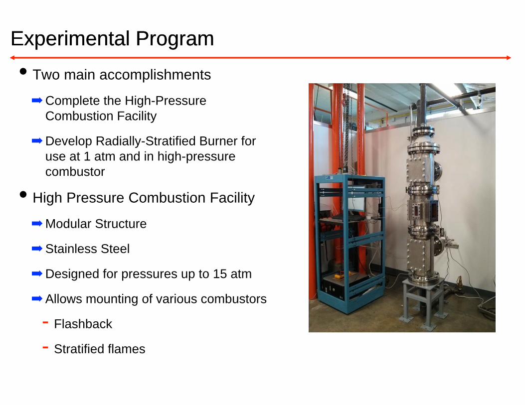
Experimental ProgramExperimental Program• Two main accomplishments
➡Complete the High-Pressure Combustion Facility
➡Develop Radially-Stratified Burner for use at 1 atm and in high-pressure combustor
• High Pressure Combustion Facility
➡Modular Structure
➡Stainless Steel
➡Designed for pressures up to 15 atm
➡Allows mounting of various combustors
- Flashback
- Stratified flames

High-Pressure Combustion FacilityHigh-Pressure Combustion Facility
High‐pressure combustion chamber
After‐cooler
Back‐pressure regulator
Exhaust piping

Lower sectionLower section
High-Pressure Combustion FacilityHigh-Pressure Combustion Facility
• Lower section
➡Access port for installation
➡Gas supply ports to the internal burner assembly

Combustion chamberCombustion chamber
High-Pressure Combustion FacilityHigh-Pressure Combustion Facility
• Combustion Chamber
➡Contains three windows for laser diagnostics
➡High-speed stereo PIV
➡Chemi-luminescence
➡PLIF
• Uses shroud air-flow for cooling windows

Upper sectionUpper section
High-Pressure Combustion FacilityHigh-Pressure Combustion Facility
• Upper Section
➡Access ports for installation and calibration

After coolerAfter cooler
High-Pressure Combustion FacilityHigh-Pressure Combustion Facility
• After cooler
➡Shell and tube heat exchanger made using copper coils

Radially-stratified Flame BurnerRadially-stratified Flame Burner
• Burner design
➡Multiple concentric tubes
- Different equivalence ratio mixtures
• Initial design with two concentric tubes
=0.9
=0.6
=0.3
air air
=1.2
=0.6
air air
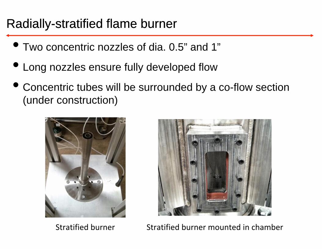
Radially-stratified flame burnerRadially-stratified flame burner
• Two concentric nozzles of dia. 0.5” and 1”
• Long nozzles ensure fully developed flow
• Concentric tubes will be surrounded by a co-flow section (under construction)
Stratified burner Stratified burner mounted in chamber

Stratified BurnerStratified Burner
• Stratified burner currently undergoing testing for flame stability with CH4-air
• Rich mixtures in both nozzles is stable at high Reynolds numbers
• Lean outer flow and rich inner flow is lifted flame for Reynolds number > 3000
• Hydrogen addition should give wider stability limits
Methane-air stratified
flame
Methane-air stratified
flame

Methane-air stratified flames at 1 atmMethane-air stratified flames at 1 atm
Inner nozzle onlyØ = 2.72, Re = 4776
Inner nozzle onlyØ = 2.72, Re = 4776
Outer nozzle only Ø = 2.12, Re = 3915
Outer nozzle only Ø = 2.12, Re = 3915
Both nozzlesInner Ø = 4.08Outer Ø = 1.9
Both nozzlesInner Ø = 4.08Outer Ø = 1.9

Planned workPlanned work
• Use H2/CH4/N2/air pre-mixtures to widen stability limits
• Make extensive measurements at 1 atm
➡PIV
➡Temperature imaging (Rayleigh scattering using DLR fuel –H2/CH4/N2)
➡OH/CH PLIF
• Make measurements at elevated-pressure conditions
Methane-air stratified
flame
Methane-air stratified
flame

LES Modeling of Flashback
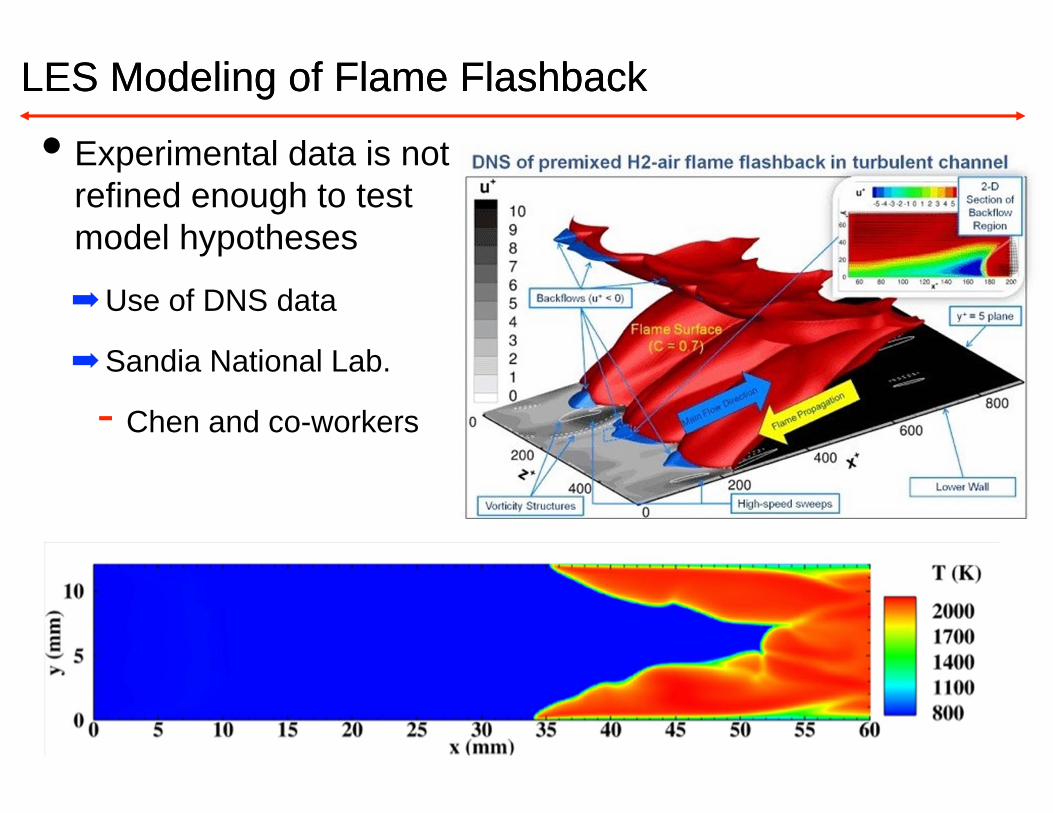
LES Modeling of Flame FlashbackLES Modeling of Flame Flashback
• Experimental data is not refined enough to test model hypotheses
➡Use of DNS data
➡Sandia National Lab.
- Chen and co-workers
Modeling ApproachModeling Approach
• Flame-front described using progress variable
➡Flame structure through flamelet model
- This is strictly not necessary
➡Progress variable source term determined to predict the correct laminar flame speed
• Modeling issues
➡Near-wall heat loss effects
➡Small-scale flame wrinkling
➡Numerical solution of the progress variable equation

DNS StatisticsDNS Statistics
• DNS represents a single realization of flashback
➡No statistical information
• Derived statistical quantities
➡Flame depth
➡Spanwise averaged flame propagation velocity
- Computed at leading edge
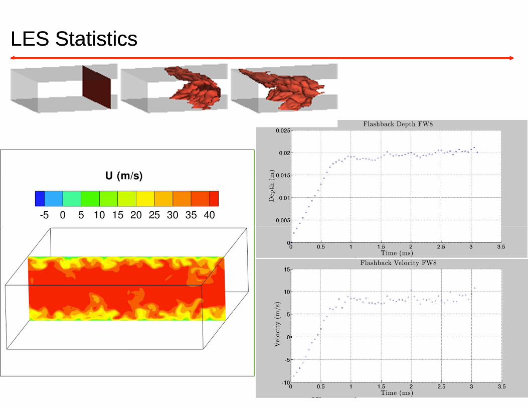
LES StatisticsLES Statistics

Flamelet Model ErrorsFlamelet Model Errors
• Flamelet assumption used to obtain progress variable source term
➡Evaluated also from DNS data

LES Results - Filter Width EffectLES Results - Filter Width Effect
• LES conducted for different grid sizes
• Filtered flame model used
➡FTACLES approach of Fiorina and co-workers
FW = Filter Width, indicates ratio of LES to DNS grid size

LES Results - Model PerformanceLES Results - Model Performance
• Different source term approximations for progress variable tested
• FTACLES approach determined to be most suitable

Moving Beyond Averages
Computational ModelingComputational Modeling
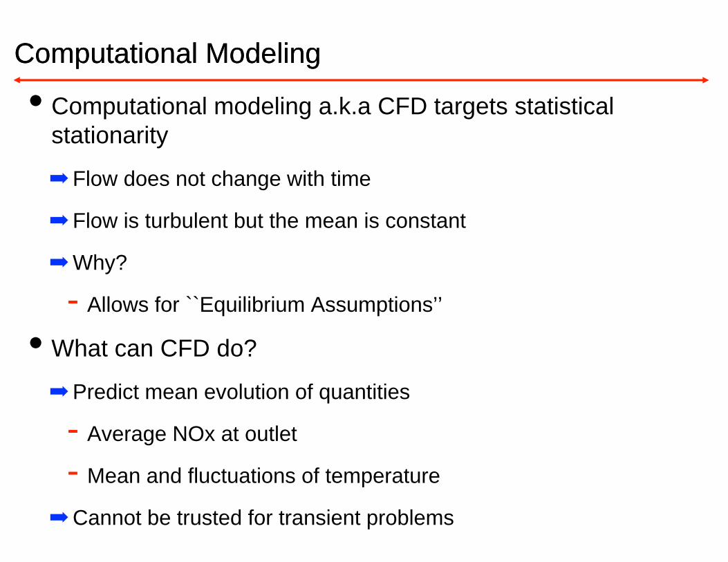
• Computational modeling a.k.a CFD targets statistical stationarity
➡Flow does not change with time
➡Flow is turbulent but the mean is constant
➡Why?
- Allows for ``Equilibrium Assumptions’’
• What can CFD do?
➡Predict mean evolution of quantities
- Average NOx at outlet
- Mean and fluctuations of temperature
➡Cannot be trusted for transient problems

Fundamentals of CFD ModelingFundamentals of CFD Modeling
• At core of all CFD models lies Equilibrium Assumption (EA)
➡Not a single assumption but spans a suite of assumptions
• Examples of EA
➡At many different scales
- Molecular thermodynamics (thermal equilibrium)
- Spectral equilibrium (turbulence and scalar spectrum are similar)
- Turbulence equilibrium (established spectrum)
• Why EA?
➡Makes modeling simpler (which is the goal of modeling)
➡Valid in many situations

EA with AveragingEA with Averaging
• All turbulence simulations use some form of averaging
➡RANS uses ensemble averaging
➡ LES uses spatial averaging followed by ensemble averaging
- The second part is not normally discussed
‣ Important for transient flow problems
• Averaging further limits the utility
➡Turbulent flow is chaotic
➡Predicting average events is useful, but not critical
➡More importantly, experiments are ideally suited for this purpose
- Simulations may not ``predict’’ new information not already obtainable
‣ Granted, experiments are expensive!

Rethinking CFD: Motivating PhysicsRethinking CFD: Motivating Physics
High Altitude Relight
Supersonic Isolator Unstart
Flame Flashback in Confined Geometries

Changing the Simulation TargetChanging the Simulation Target
• Simulations are designed to predict this:
➡What is the average speed of flashback?
• Simulations should predict this:
➡What is the probability that the flashback speed > some value?
Or
➡What is the fastest propagation speed?

Three Approaches to Understanding LESThree Approaches to Understanding LES
• Adrian (1977) provided one of the first studies on the implied meaning of filtering
➡Discussed this in terms of two different simulations approaches
➡Termed here as coarse DNS and filtered LES approaches
• Moser’s ideal LES approach (1998)
➡Similar to Adrian’s second approach
• Pope’s self-conditional LES approach (2010)
➡Seeks to restate the CFD modeling problem
➡Unique model terms arise

Statistical Definition of LESStatistical Definition of LES
• Consider a continuous velocity field
• Consider a computational grid of discrete points
➡Mesh points are spaced larger than the smallest flow scales
➡Velocity denoted by • Knowledge of alone does not determine the evolution of
➡For a given there are multiple possible transitions from to
➡Transition should be described probabilistically
• How do we evolve ?

Understanding Filtered EvolutionUnderstanding Filtered Evolution• Consider representation of velocity on a mesh
➡Wi is the vector of velocity at a given point
Wi

Multi-point Probability Density FunctionMulti-point Probability Density Function
• Consider the following event
➡ n refers to the number of grid points in the computational grid
➡The event refers to multi-point velocity information
• The joint-PDF evolves according to
• The best solution from the LES reproduces the multi-point PDF accurately
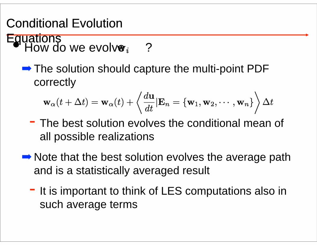
Conditional Evolution EquationsConditional Evolution Equations• How do we evolve ?
➡The solution should capture the multi-point PDF correctly
- The best solution evolves the conditional mean of all possible realizations
➡Note that the best solution evolves the average path and is a statistically averaged result
- It is important to think of LES computations also in such average terms
Developing Conditional Models in LESDeveloping Conditional Models in LES
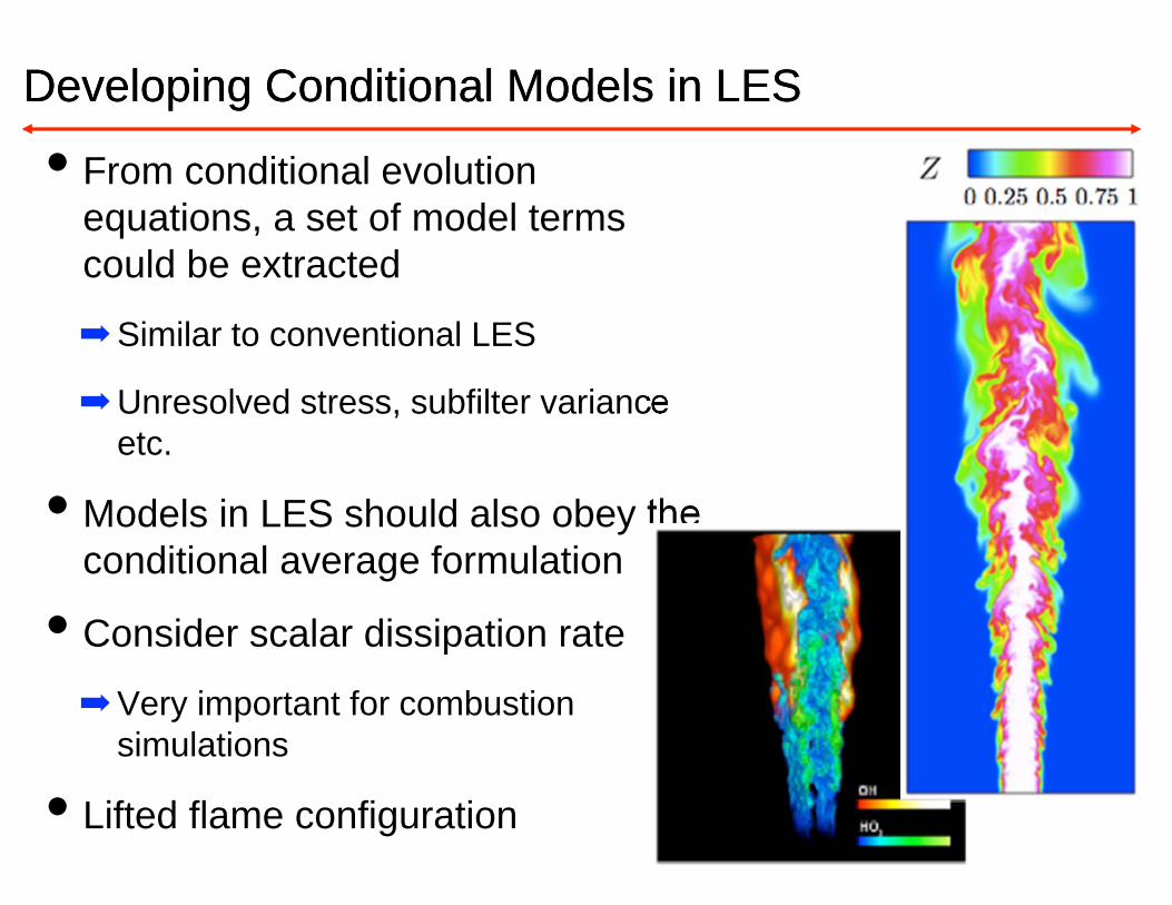
• From conditional evolution equations, a set of model terms could be extracted
➡Similar to conventional LES
➡Unresolved stress, subfilter variance etc.
• Models in LES should also obey the conditional average formulation
• Consider scalar dissipation rate
➡Very important for combustion simulations
• Lifted flame configuration

Conditionally Averaged Combustion ModelsConditionally Averaged Combustion Models
• New optimal estimator based model selection
➡Provides an estimate of the least error that could be made with a given set of input variables
➡Model form chosen to be close to this error
DNS LES
From Kaul et al. (2013), Proc. Comb. Inst.

Multi-time FormulationsMulti-time Formulations
• CFD has to move beyond one-point one-time models
➡Multi-time models for transient flow behavior
• Current project
➡Understand variability in flashback
➡Devise modeling methods for predicting ``extreme events”
➡Map the limitations of LES in predicting such transient flows

Constrained Premixed FlameConstrained Premixed Flame
• Flame propagation in homogeneous isotropic turbulence
• Flame location fixed using a control loop

Position Control AlgorithmPosition Control Algorithm
• Flame position adjusted by changing inflow velocity
➡Response time adjusted to ensure stability
➡Total adjustment a small fraction of the flame propagation velocity
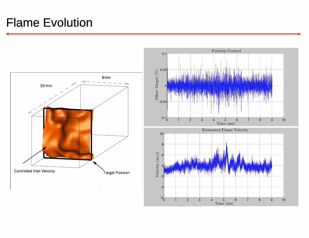
Flame EvolutionFlame Evolution

PDF of Flame Propagation VelocityPDF of Flame Propagation Velocity
• Strong asymmetry in flame propagation
➡Faster velocities are more common than slower velocities

ConclusionsConclusions
• High-pressure setup constructed
➡ Initial stratified flame studies underway
• LES of flashback
➡Progress variable approach predicts DNS statistics reasonably accurately
➡Flame wrinkling effects at larger filter widths need to be studied
• New modeling strategy for CFD
➡Towards probabilistic modeling of transient flows
➡Homogeneous cases used to understand time correlation of extreme events