Large Panel Test of Factor Pricing Models

Jianqing Fan ∗†, Yuan Liao‡and Jiawei Yao∗

∗Department of Operations Research and Financial Engineering, Princeton University

† Bendheim Center for Finance, Princeton University

‡ Department of Mathematics, University of Maryland

Abstract

We consider testing the high-dimensional multi-factor pricing model, with the num-

ber of assets much larger than the length of time series. Most of the existing tests are

based on a quadratic form of estimated alphas. They suffer from low powers, however,

due to the accumulation of errors in estimating high-dimensional parameters that over-

rides the signals of non-vanishing alphas. To resolve this issue, we develop a new class

of tests, called “power enhancement” tests. It strengthens the power of existing tests

in important sparse alternative hypotheses where market inefficiency is caused by a

small portion of stocks with significant alphas. The power enhancement component is

asymptotically negligible under the null hypothesis and hence does not distort much

the size of the original test. Yet, it becomes large in a specific region of the alter-

native hypothesis and therefore significantly enhances the power. In particular, we

design a screened Wald-test that enables us to detect and identify individual stocks

with significant alphas. We also develop a feasible Wald statistic using a regularized

high-dimensional covariance matrix. By combining those two, our proposed method

achieves power enhancement while controlling the size, which is illustrated by extensive

simulation studies and empirically applied to the components in the S&P 500 index.

Our empirical study shows that market inefficiency is primarily caused by merely a few

stocks with significant alphas, most of which are positive, instead of a large portion of

slightly mis-priced assets.

∗Address: Department of Operations Research and Financial Engineering, Sherrerd Hall, Princeton Uni-versity, Princeton, NJ 08544, USA. Department of Mathematics, University of Maryland, College Park,MD 20742, USA. E-mail: jqfan@princeton.edu, yuanliao@umd.edu, jiaweiy@princeton.edu. The research waspartially supported by DMS-1206464, NIH R01GM100474-01 and NIH R01-GM072611.

1

arX

iv:1

310.

3899

v1 [

stat

.ME

] 1

5 O

ct 2

013

Keywords: high dimensionality, approximate factor model, test for mean-variance effi-

ciency, power enhancement, thresholding, covariance matrix estimation, Wald-test, screening

JEL code: C12, C33, C58

2

1 Introduction

Factor pricing model is one of the most fundamental results in finance. It postulates how

financial returns are related to market risks, and has many important practical applications,

including portfolio selection, fund performance evaluation, and corporate budgeting. It also

includes the Capital Asset Pricing Model (CAPM) as a specific case.

The multi-factor pricing model was derived by Ross (1976) using the arbitrage pricing

theory and by Merton (1973) using the Intertemporal CAPM. Let yit be the excess return of

the i-th asset at time t and f t = (f1t, ..., fKt)′ be the excess returns of K market risk factors.

Then, the excess return has the following decomposition:

yit = αi + b′ift + uit, i = 1, ..., N, t = 1, ..., T, (1.1)

where bi = (bi1, ..., biK)′ is a vector of factor loadings and uit represents the idiosyncratic

error. The key implication from the multi-factor pricing theory is that the intercept αi

should be zero, known as “mean-variance efficiency”, for any asset i. An important question

is then if such a pricing theory can be validated by empirical data, namely whether the null

hypothesis

H0 : α = 0, (1.2)

is consistent with empirical data, where α = (α1, ..., αN)′ is the vector of intercepts for all

N financial assets.

Most of the existing tests to the problem (1.2) are based on the quadratic statistic

W = α′Vα, where α is the OLS estimator for α, and V is some positive definite matrix.

The Wald statistic, for instance, takes the form aT α′Σ−1

u α, where Σ−1u is the estimated

inverse of the error covariance, and aT is a positive number that depends on the factors ft

only. Other prominent examples are the test given by Gibbons, Ross and Shaken (1989,

GRS test), the GMM test in MacKinlay and Richardson (1991), and the likelihood ratio

test in Beaulieu, Dufour and Khalaf (2007, BDK test), all in quadratic forms. See Sentana

(2009) for an overview.

The above tests are applicable only when the number of assets N is much smaller than the

length of the time series T . When N ≥ T , for instance, the sample covariance Σu becomes

degenerate. However, one typically picks a testing period of T = 60 monthly data and does

not increase the testing period any longer, because the factor pricing model is technically a

one-period model whose factor loadings can be time-varying. As a result, it would often be

3

the case when the number of assets N is much larger than T . To overcome the difficulty,

Pesaran and Yamagata (2012, PY test) proposed to ignore the correlations among assets

and constructed a test statistic under working independence: choosing V = diag(Σu)−1 to

avoid the issue of invertibility. They obtained the asymptotic normality of the standardized

quadratic form: (W − EW )/√

var(W ). A closely related idea was employed by Chen and

Qin (2010) and Chen, Zhang and Zhong (2010) to ameliorate high-dimensional Hotelling

test. However, even such a simplified quadratic test suffers from a low power in a high-

dimension-low-sample-size situation, as we now explain.

For simplicity, let us temporarily assume that utTt=1 are i.i.d. Gaussian and Σu =

cov(ut) is known, where ut = (u1t, ..., uNt). In this case, the Wald test statistic W equals

T α′Σuα times a constant that only depends on the factors. Under H0, it is χ2N distributed,

with the critical value χ2N,q , which is of order N , at significant level q. The test has no power

at all when Tα′Σuα = o(N) or ‖α‖2 = o(N/T ), assuming that Σu has bounded eigenvalues.

This is not unusual for the high-dimension-low-sample-size situation we encounter, where

there are thousands of assets to be tested over a relatively short time period (e.g. 60 monthly

data). And it is especially the case when there are only a few significant alphas that arouse

market inefficiency. By a similar argument, this problem can not be rescued by using the PY

test, or any other genuine quadratic statistic, which are powerful only when a non-negligible

fraction of assets are mispriced. Indeed, the factor N above reflects the noise accumulation

in estimating N parameters of α.

We resolve the above problem by introducing a novel technique, called the “power en-

hancement” (PEM) technique. Let J1 be a test statistic that has a correct asymptotic size

(e.g., GRS, PY, BDK), which may suffer from small powers in all directions. Let us augment

the test by adding a PEM component J0 ≥ 0 with the following two properties:

(a) Under H0, J0 has an order of magnitude smaller than J1. If J1 has been normalized,

this requires that J0P→ 0 under H0.

(b) J0 does not converge to zero and even diverges when the true parameters fall in a

subset Θ of the alternative hypothesis.

The constructed PEM test is then of the form

J = J0 + J1. (1.3)

Property (a) shows that the size distortion is negligible, property (b) guarantees significant

4

power improvement on the set Θ, and the nonnegativity property of J0 ensures that J is

always at least as powerful as J1.

As an example, we construct a screened Wald-test defined by

J0 = α′SVSαS (1.4)

where αS = (αj : |αj| > δT ) is a subvector of α whose individual magnitude exceeds the

threshold δT , and VS is the corresponding submatrix of a weight matrix V. The threshold

δT is chosen such that under the null hypothesis,

P (J0 = 0|H0)→ 1,

and that J0 diverges when maxj≤N |αj| δT . This enhances the power of J1 in the sparse

alternatives. The PEM component can be combined with either the PY test or the Wald

test; the latter needs further development when N > T .

Another contribution of the paper is to develop an operational Wald statistic even when

N/T →∞ and Σu is non-diagonal. The statistic is based on a regularized sparse estimator

of Σu. We show that as N, T → ∞, with the covariance estimator Σ−1u , the standardized

Wald test

Jsw =aT α

′Σ−1u α−N√2N

→d N (0, 1)

under the null hypothesis for a given normalization factor aT . This feasible test takes into

account the cross-sectional dependence among the idiosyncratic errors. Technically, in order

to show that the effect of replacing Σ−1u with the sparse estimator Σ−1

u is negligible, we need

to establish, under H0,

aT α′(Σ−1

u −Σ−1u )α = oP (

√N). (1.5)

Note that a simple inequality |α′(Σ−1u −Σ−1

u )α| ≤ ‖α‖2‖Σ−1u −Σ−1

u ‖ yields a too crude bound

of order O(N/T ), due to the error accumulation in ‖α‖2 under high dimensions. Instead,

we have developed a new technical strategy to prove (1.5), which would also be potentially

useful in high-dimensional inference using GMM methods when one needs to estimate the

optimal weight matrix of high dimensions. We further take J1 = Jsw, and combine it with

our PEM J0 in (1.4) to propose a power enhancement test. It is much more powerful than

existing tests, while maintaining the same asymptotic null distribution. We show that the

power is enhanced uniformly over the true α.

5

Moreover, the screening step in the construction of J0 also identifies the individual stocks

with significant alphas. They provide us useful information on which stocks are mis-priced

and contribute importantly to the market inefficiency. In contrast, most of the existing tests

do not possess this feature.

The proposed methods are applied to the securities in the S&P 500 index as an empirical

application. The empirical study shows that market inefficiency is indeed primarily caused

by a small portion of mis-priced stocks instead of systematic mis-pricing of the whole mar-

ket. Most of the significant alphas are positive, which result in extra returns. The market

inefficiency is further evidenced by our newly created portfolio based on the PEM test, which

outperforms the S&P500 index.

Importantly, the proposed PEM is widely applicable in many high-dimensional testing

problems in applied econometrics. For instance, in panel data models

yit = x′itβi + ηi + uit,

we are often interested in testing slope homogeneity H0 : βi = β,∀i ≤ N (e.g., Phillips

and Sul 2003, Breitung et al. 2013), and cross-sectional independence H0 : cov(uit, ujt) =

0,∀i 6= j (Baltagi et al. 2012, Sarafidis et al. 2009, Pesaran et al. 2008). The proposed

PEM principle carries over to these cases.

It is worth pointing out that in the statistical literature, there are many studies on testing

the mean vector of a high-dimensional Gaussian vector (e.g., Hall and Jin 2010, Srivastava

and Du 2008, etc.). These methods are not applicable here because they are mainly concerned

with a special type of sparse alternatives, where the correlations among observations should

decay fast enough. In contrast with our settings here, their estimated alphas can be strongly

correlated.

The remainder of the paper is organized as follows. Section 2 sets up the preliminaries

and discusses the limitations of traditional tests. Section 3 proposes the power enhance-

ment method, derives the asymptotic behaviors of the screening statistic and analyzes its

performances under different alternatives. Section 4 combines the PEM with the working-

independent quadratic form. Section 5 studies a high-dimensional Wald-test. Section 6

discusses extended applications of PEM in panel data models and GMM. Simulation results

are presented in Section 7, along with an empirical application to the stocks in the S&P 500

index in Section 8. Section 9 concludes. All the proofs are given in the appendix.

Throughout the paper, for a square matrix A, let λmin(A) and λmax(A) represent its

6

minimum and maximum eigenvalues. Let ‖A‖ and ‖A‖1 denote its operator norm and l1

norm respectively, defined by ‖A‖ = λ1/2max(ATA) and maxi

∑j |Aij|. For two deterministic

sequences aT and bT , we write aT bT (or equivalently bT aT ) if aT = o(bT ). Also,

aT bT if there are constants C1, C2 > 0 so that C1bT ≤ aT ≤ C2bT for all large T . Finally,

we denote |S|0 as the number of elements in a set S.

2 Factor models and traditional tests

The multi-factor model (1.1) can be more compactly expressed as

yt = α + Bft + ut, t = 1, ..., T,

where yt = (y1t, ..., yNt)′ is the excess return vector at time t; B = (b1, ...,bN)′ is a loading

matrix, and ut = (u1t, ..., uNt) denotes the idiosyncratic component. Here both yt and ft are

observable. Our goal is to test the hypothesis

H0 : α = 0,

namely the multi-factor pricing model is consistent with the data. As argued in the intro-

duction, we are particularly interested in a high-dimensional situation where N = dim(α)

can be much larger than T , that is, N/T →∞.We set up the model to have an approximate factor structure as in Chamberlain and

Rothschild (1983), in which the covariance matrix Σu = cov(ut) is sparse. Since the common

factors have substantially mitigated the co-movement across the whole panel, a particular

asset’s idiosyncratic volatility is usually correlated significantly only with a couple of other

assets. For example, some shocks only exert influences on a particular industry, but are not

pervasive for the whole economy (Connor and Korajczyk, 1993). Such a sparse assumption

enables us to reliably estimate the error covariance later.

7

2.1 Wald-type tests

We can run OLS for regressions stock by stock to estimate α. Denote by f = 1T

∑Tt=1 ft,

w = ( 1T

∑Tt=1 ftf

′t)−1f , and aT = T (1− f ′w). Then, the OLS estimator can be expressed as

α = (α1, ..., αN)′, αi = a−1T

T∑t=1

yit(1− f ′tw).

Simple calculations yield

αi = αi + a−1T

T∑t=1

uit(1− f ′tw).

Assuming no serial correlation among utTt=1, the conditional covariance of α is Σu/aT ,

given the factors. If Σu is known, the classical Wald test statistic is

W = aT α′Σ−1

u α. (2.1)

When N < T − K − 1 (recall K = dim(ft)), Σu can be estimated and replaced by the

sample covariance matrix of the residual vector, and the resulting test statistic is then in line

with the well-known test by Gibbons et al. (1989, GRS). Under the Gaussian assumption,

GRS obtained the exact finite sample distribution of this test statistic. The asymptotic null

distribution is χ2N -distribution when N is fixed. When N diverges, the traditional asymptotic

theory for W does not apply directly. Instead, Pesaran and Yamagata (2012) developed an

alternative asymptotic null distribution for the Wald statistic. They showed that under some

regularity conditions,

J1 =aT α

′Σ−1u α−N√2N

→d N (0, 1). (2.2)

as N → ∞. Hence at the significant level q ∈ (0, 1), P (J1 > zq|H0) → q with critical value

zq.

Regardless of the type of asymptotics, we shall refer to the test based on W (with Σ−1u

possibly replaced with an estimator Σ−1u ) as a Wald-type statistic, or quadratic test because

W is a quadratic form of α.

2.2 Two main challenges of quadratic test

In a data-rich environment, the panel size N can be much larger than the number of

observations T . Such a high dimensionality brings new challenges to the test statistics based

8

on W , and the alternative asymptotics (2.2) only partially solves the problem. Specifically,

there are two main challenges.

The first challenge arises from estimating Σ−1u in the presence of error cross-sectional

correlations. It is well known that the sample residual covariance matrix becomes singular

when N > T −K − 1. Even if N < T −K − 1, replacing Σ−1u in W with the inverse sample

covariance can still bring a huge amount of estimation errors when N2 is close to T . This

can distort the null distribution of the test statistic when the data deviates slightly from the

normality.

Another challenge comes from the loss of power due to estimating the high-dimensional

parameter vector α. Even when Σ−1u is known so that W is feasible, it still has very low

powers against various alternative hypotheses when N is large. This again can be ascribed

to the noise accumulation as illustrated in the following example.

Example 2.1. Suppose that Σu = IN , the identity matrix, and the data are serially indepen-

dent. Conditioning on the observed factors, W is distributed as χ2N(aT‖α‖2), a non-central

χ2-distribution with degree of freedom N and noncentrality parameter aT‖α‖2. Under the

null hypothesis, W ∼ χ2N , which has mean N and standard deviation

√2N . Now, consider

the power of the test at the alternative, for some r < N ,

Ha : αi = 0, for i > r.

Then, the test statistic W ∼ χ2N(aT

∑ri=1 α

2i ) under Ha, which has mean aT

∑ri=1 α

2i + N .

Thus, if all αi’s are bounded, the test statistic has no power against Ha when rT/√N = o(1)

or r = o(√N/T ).

In the previous example, there are only a few non-vanishing alphas in the alterna-

tive, whose signals are dominated by the aggregated high-dimensional estimation errors:

T∑

i>r α2i . On the other hand, the first r assets with non-vanishing alphas (fixed constants)

are actually detectable (e.g., by confidence intervals) when (logN)/T converges, which should

be considered when constructing the test. The above simple example illustrates how noise

accumulation of the Wald test masks the power of the test. Such a result holds more generally

as shown in the following Theorem.

Theorem 2.1. Suppose that Assumption 3.2 below holds, and both ‖Σu‖1 and ‖Σ−1u ‖1 are

9

bounded. When T = o(√N), the test J1 in (2.2) has low power at the following alternative:

Ha : there are at most r = o(

√N

T) non-vanishing but bounded αj’s.

More precisely, P (J1 > zq|Ha) ≤ 2q + o(1) for any significant level q ∈ (0, 0.5).

A more sensible approach is to focus on those alternatives that may have only a few

nonzero alphas compared to N . This is particularly interesting when the market inefficiency

is primarily caused by a minority of mis-priced stocks rather than systematic mis-pricing of

the whole market. In what follows, we develop a new testing procedure that significantly

improves the power of the Wald-type test against such sparse alternatives.

3 Power Enhancement

Traditional tests of factor pricing models are not powerful unless there are enough stocks

that have non-vanishing alphas. Even if some individual assets are significantly mis-priced,

their non-trivial contributions to the test statistic are insufficient to reject the null hypothesis.

This problem can be resolved by introducing a power enhancement component (PEM) J0

to the traditional test J1 as in (1.3). The PEM J0 is designed to detect sparse alternatives

with significant individual alphas.

3.1 Screened Wald Statistic

To prevent the accumulation of estimation errors in a large panel, we propose a screened

test statistic. For some predetermined threshold value δT > 0, define a set

S =

j :|αj|σj

> δT , j = 1, ..., N

, (3.1)

where αj is the OLS estimator and σ2j =

∑Tt=1 u

2jt/aT is T times the estimated variance of

αj, with ujt being the regression residuals. Denote a subvector of α by

αS = (αj : j ∈ S),

the screened-out alpha estimators, which can be interpreted as estimated alphas of mis-priced

stocks. Let Σu be a consistent estimator of Σu to be defined later, and ΣS the submatrix

10

of Σu formed by the rows and columns whose indices are in S. So ΣS/aT is an estimated

conditional covariance matrix of αS, given the common factors and S.

With the above notation, we define our screened Wald statistic as

J0 =√NaT α

′SΣ−1

SαS, (3.2)

where aT = T (1 − f ′w). A similar idea of this kind of thresholding test appears in Fan

(1996). The choice of δT must suppress most of the noises, resulting in an empty set of S

under the null hypothesis. On the other hand, δT cannot be too large to filter out important

signals of alphas under the alternative. For this purpose, noting that the maximum noise

level is OP (√

logN/T ), we let

δT = log(log T )

√logN

T.

With this choice of δT , if we define, for σ2j = (Σu)jj/(1− Ef ′t(Eftf

′t)−1Eft),

S =

j :|αj|σj

> 2δT , j = 1, ..., N

, (3.3)

then under mild conditions, P (S = S)→ 1, and αS behaves like αS = (αj : j ∈ S).

The screened Wald statistic depends on a nonsingular covariance matrix Σ−1

Sthat con-

sistently estimates Σ−1S . The matrix ΣS is a submatrix of Σu corresponding to the indices in

S, and can be large when the set S is large. So it is difficult to estimate in general. To obtain

an operational Σ−1

S, we assume Σu to be sparse and estimate it by thresholding (Bickel and

Levina, 2008). For the sample covariance sij = 1T

∑Tt=1 uitujt, let the thresholded sample

covariance as

(Σu)ij =

sij, if i = j,

θij(sij), if i 6= j,(3.4)

where θij(·) is a generalized thresholding function (Antoniadis and Fan, 2001, Rothman et

al. 2009), with threshold value hij = C(siisjjlogNT

)1/2 for some constant C > 0, designed to

keep the sample correlation whose magnitude exceeds C( logNT

)1/2. In particular, when the

hard-thresholding function θij(x) = x1|x| > hij is used, this is the estimator proposed by

Fan et al. (2011). Many other thresholding functions such as soft-thresholding and SCAD

can also be employed. In general, θij(·) should satisfy (Antoniadis and Fan, 2001):

11

(i) θij(z) = 0 if |z| < hij;

(ii) |θij(z)− z| ≤ hij;

(iii) there are constants a > 0 and b > 1 such that |θij(z)− z| ≤ ah2ij if |z| > bhij.

The thresholded error covariance matrix estimator sets most of the off-diagonal estimation

noises in ( 1T

∑Tt=1 uitujt) to zero, and produces a strictly positive definite matrix even when

N > T . The constant C in the threshold can be selected in a data-driven way, which we

refer to Fan et al. (2013) and Cai and Liu (2011). Moreover, it can be shown that Σ−1u

consistently estimates Σ−1u under the operator norm.

Alternatively, we can use the working-independent version of the quadratic statistic,

replacing ΣS by DS = diagsjj : j ∈ S. This is particularly convenient when Σu is close to

diagonal, and corresponds to taking hij = (siisjj)1/2 in the thresholded covariance estimator

with the hard-thresholding rule. The screening working-independent test statistic is then

defined as

J0 =√NaT αSD−1

SαS =

√NaT

∑j∈S

α2js−1jj . (3.5)

3.2 Power enhancement test

The screened statistic J0 is powerful in detecting stocks with large individual alphas.

However, J0 equals zero with probability approaching one under the null hypothesis. Hence,

it can not live on its own to obtain the right size of the test, but can be combined with any

other standard test statistics to achieve a proper size.

Suppose J1 is a test statistic for H0 : α = 0 and it has high power on a subset Ω1 ⊂ RN \0.

Our power enhancement test is simply

J = J0 + J1.

Since J0 = 0 with probability approaching one under the null hypothesis, the null distribution

of J is asymptotically determined by that of J1. Let Fq be the critical value for J1 under

the significant level q, that is, P (J1 > Fq|H0) ≤ q. Our proposed PEM J-test then rejects

H0 when J > Fq. The size is not much distorted since

P (J > Fq|H0) = P (J1 > Fq|H0) + o(1) ≤ q + o(1).

12

Since J ≥ J1, the power of the enhanced test J is no smaller than that of J1. On the other

hand, if J0 has high power on a subset Ω0 ⊂ RN \ 0 in the sense that J0P→ ∞ for α ∈ Ω0,

then J has power approaching one on the set Ω0. In other words, we show that the PEM

J-test has high power uniformly on the region Ω0 ∪ Ω1. The power is enhanced whenever

Ω0 ∪ Ω1 is strictly larger than Ω1. In high-dimensional testing problems, due to the error

accumulations, Ω0 and Ω1 can be quite different.

To formally establish the aforementioned power enhancement properties, we need the

sparsity of Σu in order for the thresholded covariance matrix estimator to work. This leads

to defining a generalized sparsity measure

mN = maxi≤N

N∑j=1

|(Σu)ij|k, for some k ∈ [0, 1). (3.6)

Note that when k = 0, mN is the maximum number of non-vanishing entries in each row (or

column, with usual convention 00 = 0). We assume logN = o(T ) and that

Assumption 3.1. There is k ∈ [0, 1) such that

mN = o

((

T

logN)(1−k)/2

).

Under the above generalized sparsity assumption, the thresholded covariance estimator

Σu is positive definite, and consistently estimates Σu under the operator norm. When

Σu is block diagonal with finite block sizes, Assumption 3.1 holds with bounded mT for

any k ∈ [0, 1). Sparsity is one of the commonly used assumptions on high-dimensional

covariance matrix estimation, which has been extensively studied recently. We refer to El

Karoui (2008), Bickel and Levina (2008), Lam and Fan (2009), Cai and Liu (2011), and the

references therein.

Let F0−∞ and F∞T denote the σ-algebras generated by (ft,ut) : −∞ ≤ t ≤ 0 and

(ft,ut) : T ≤ t ≤ ∞ respectively. In addition, define the α-mixing coefficient

α(T ) = supA∈F0

−∞,B∈F∞T|P (A)P (B)− P (AB)|.

Assumption 3.2. (i) Strict stationarity: ft,utt≥1 is strictly stationary, Eut = 0 and

Eutft = 0. In addition, for s 6= t, Eutu′s = 0, and Ef ′t(Eftf

′t)−1Eft < 1.

13

(ii) There exist constants c1, c2 > 0 such that maxi≤N ‖bi‖ < c2,

c1 < λmin(Σu) ≤ λmax(Σu) < c2, and c1 < λmin(cov(ft)) ≤ λmax(cov(ft)) < c2.

(iii) Exponential tail: There exist r1, r2 > 0, and b1, b2 > 0, such that for any s > 0,

maxi≤N

P (|uit| > s) ≤ exp(−(s/b1)r1), maxi≤K

P (|fit| > s) ≤ exp(−(s/b2)r2).

(iv) Strong mixing: There exists r3 > 0 such that r−11 +r−1

2 +r−13 > 1, and C > 0 satisfying:

for all T ∈ Z+,

α(T ) ≤ exp(−CT r3).

These conditions are standard in the time series literature. In Condition (i), we require

the idiosyncratic error ut be serially uncorrelated across t. Under this condition, the condi-

tional covariance of α is Σu/aT given the factors. Estimating Σu when N > T is already

challenging. When the serial correlation is present, the autocovariance of ut would also be

involved in the covariance of the OLS estimator for alphas, and needs be estimated. We

rule out these autocovariance terms to simplify the technicalities, and our method can be

extended to the case with serial correlation. On the other hand, we allow the factors to

be weakly dependent via the strong mixing condition, which holds when factors follow a

VAR model. Also, it is always true that Ef ′t(Eftf′t)−1Eft ≤ 1. We rule out the equality to

guarantee that the asymptotic variance of√T αj does not degenerate for each j.

The following theorem quantifies the asymptotic behavior of the screening Wald statistic

J0, and provides sufficient conditions for the selection consistency. Recall that S and S are

defined in (3.1) and (3.3) respectively. Define the “grey area set” as

G = j : αj δT , j = 1, ..., N.

Theorem 3.1. Suppose logN = o(T ), Assumption 3.2 hold. As T,N →∞,

P (S ⊂ S)→ 1, P (S \ S ⊂ G)→ 1.

In addition, under the null hypothesis, P (S = ∅)→ 1. Hence

P (J0 = 0|H0)→ 1,

14

We are particularly interested in a type of alternative hypothesis that satisfy the following

empty grey area condition.

Assumption 3.3. Empty grey area: The alternative hypothesis Ha satisfies G = ∅.

The empty grey area represents a class of alternatives that have no nonzero αj’s on

the boundary of the screening set S. This condition is weak because the chance of falling

exactly at the boundary is very low. Intuitively speaking, when an αj is on the boundary

of the screening, it is hard to decide whether to eliminate it from the screening step or not.

According to Theorem 3.1, the difference between the set estimator S and the oracle set S

is contained in the grey area G with probability approaching one.

Corollary 3.1. Under the assumptions of Theorem 3.1 and Assumption 3.3, we have

P (S = S)→ 1.

Note that the set S contains all individual stocks with large value of alphas and is the

set of stocks that we wish to identify. Theorem 3.1 shows that they can be identified with

no missing discoveries and Corollary 3.1 further asserts that the identification is consistent

with no false discoveries either.

Define

Ω0 = α ∈ RN : maxj≤N|αj| > 2δT max

j≤Nσj.

Below we write P (·|α) to denote the probability measure if the true alpha is α. A test is

said to have high power uniformly on a set A ⊂ RN \ 0 if infα∈A P (reject|α)→ 1.

We now present the asymptotic behavior of the PEM test.

Theorem 3.2. Suppose logN = o(T ), and Assumptions 3.1-3.3 hold. In addition, suppose

there is a test J1 such that (i) it has an asymptotic non-degenerate null distribution F ;

(ii) its critical region takes the form J1 > Fq for the level q ∈ (0, 1), and (iii) it has high

power uniformly on some set Ω1. Then the PEM test J = J0 + J1 has the asymptotic null

distribution F and high power uniformly on the set Ω0 ∪ Ω1:

infα∈Ω0∪Ω1

P (J > C|α)→ 1.

Theorem 3.2 shows that J1 and J both have the critical regions J > Fq and J1 > Fq

respectively, where Fq is the qth quantile of F . It follows immediately from J ≥ J1 that

15

P (J > Fq|α) ≥ P (J1 > Fq|α), which means J is at least as powerful as J1. In addition, J0

plays exactly the role of power enhancement, in the sense that (i) it does not affect much

the null distribution, and (ii) it substantially increases the power on Ω0.

4 PEM for working-independent quadratic test

PEM can be combined with many tests. In this section, we consider the working-

independent quadratic test recently developed by Pesaran and Yamagata (2012) in the cur-

rent context. Without PEM, Theorem 2.1 shows that the working-independent test can

suffer from low powers in high-dimensional testing problems.

4.1 Working-independent quadratic statistic

To avoid the degeneracy of the sample covariance Σu in normalizing the Wald statistic,

one can simply ignore the cross-sectional correlations and utilize the diagonal matrix D =

diag(Σu) to normalize the quadratic form:

W = aT α′D−1α, D = diags11, ..., sNN.

Note that W is a sum of N correlated individual squared t-statistics. One needs to calculate

and estimate both E(W ) and var(W ) under the null hypothesis in order to establish the

asymptotic normality. As D ignores the off-diagonal entries of Σu, W is no longer χ2 even

under the normal assumption when Σu is indeed non-diagonal. Hence, efforts are needed to

calculate the first two moments of W . This has been achieved by Pesaran and Yamagata

(2012) and leads to a feasible version of the normalized test:

Jwi =W −N√

2N(1 + eT )(4.1)

where

eT = N−1∑i 6=j

ρ2ijI(ρ2

ij > cT ) with cT =1

TΦ−1(1− c/N)

for some c ∈ (0, 0.5). Here ρij denotes the sample correlation between uit and ujt based on the

residuals, and Φ−1(·) denotes the inverse standard normal cumulative distribution function.

Applying a linear-quadratic form central limit theorem (Kelejian and Prucha 2001), it can

be shown that Jwi is asymptotically standard normal, as N, T → ∞. We call Jwi as the

16

working-independent quadratic statistic. Pesaran and Yamagata (2012) proposed a slightly

different (but asymptotically equivalent) statistic that corrects the finite sample bias. For

example, the expected value of squared t-statistic with degree of freedom ν is ν/(ν − 2).

Therefore, the numerator of (4.1) should be centerized by N(N − K − 1)/(N − K − 3)

instead of N .

4.2 Asymptotic results

We now study the power of the PEM test J = J0 + Jwi where J0 is given by either (3.2)

or (3.5). It is summarized in the following theorem.

Theorem 4.1. Suppose logN = o(T ) and Assumptions 3.1-3.3 hold. Also,∑

i 6=j(Σu)2ij =

O(N). As N, T →∞ and N/T 3 → 0, we have

(i) under the null hypothesis H0 : α = 0, J →d N (0, 1),

(ii) PEM test J has high power uniformly on the set

Ω0 ∪ α ∈ RN : ‖α‖2 (N logN)/T ≡ Ω0 ∪ Ω1,

that is, for any q ∈ (0, 1), infα∈Ω0∪Ω1 P (J > zq|α)→ 1.

We see that including J0 in the PEM test does not alter the asymptotic null distribution,

but it significantly enhances the power of Jwi on the set Ω0. The set

Ω1 = α ∈ RN : ‖α‖2 (N logN)/T itself is the region where Jwi has a high power, but

this is a restrictive region when N > T . For instance, it rules out the type of alternatives in

which there are finitely many non-vanishing alphas, but such a sparse scenario is included

in Ω0. Hence, the PEM J will be able to detect it.

5 High-dimensional Wald test and its PEM

The working-independent quadratic test is a simple way of dealing with the singularity

of the sample covariance matrix of ut when N > T , and to avoid estimating the high-

dimensional covariance matrix Σu. On the other hand, when Σu were known, one typically

prefers the Wald test or equivalently its normalized version

aT α′Σ−1

u α−N√2N

, (5.1)

17

which has an asymptotic null distribution N (0, 1). A natural question is that when Σu

admits a sparse structure, can it be estimated accurately enough for a substitution into

(5.1)? The answer is affirmative if N logN = o(T 2), and still we can allow N/T → ∞.

However, such a simple question is far more technically involved than anticipated, as we now

explain.

5.1 A technical challenge

When Σu is a sparse matrix, Fan et al. (2011) obtained a thresholded estimator Σu as

described in Section 3.1, which satisfies

‖Σ−1u − Σ−1

u ‖ = OP (mN

√logN

T), (5.2)

where mN = maxi≤N∑N

j=1 1(Σu)ij 6= 0. Using the lower bound derived by Cai and Zhou

(2012), we infer that the convergence rate is minimax optimal for the sparse covariance

estimation.

When replacing Σ−1u in (5.1) by Σ−1

u , one needs to show that the effect of such a replace-

ment is asymptotically negligible, namely, under H0,

T α′(Σ−1u − Σ−1

u )α/√N = oP (1).

Note that when α = 0, with careful analysis, ‖α‖2 = OP (N/T ). Using this and (5.2), by

the Cauchy-Schwartz inequality, we have

|T α′(Σ−1u − Σ−1

u )α|/√N = OP (mN

√N logN

T).

We see that even if mN is bounded, it still requires N logN = o(T ), which is basically a

low-dimensional scenario.

The above simple derivation uses, however, a very crude Cauchy-Schwartz bound, which

accumulates too many estimation errors in ‖α − α‖2 (with α = 0 under H0) under a

large N . In fact, α′(Σ−1u − Σ−1

u )α is a weighted estimation error of Σ−1u − Σ−1

u , where the

weights α “average down” the accumulated estimation errors, and result in an improved

rate of convergence. The formalization of this argument requires subtle technical details and

further regularity conditions. These are formally presented in the following subsection.

18

5.2 Wald test and power enhancement

To simplify our discussion, let us focus on the serially independent Gaussian case.

Assumption 5.1. Suppose:

(i) ut is distributed as N (0,Σu), where both ‖Σu‖1 and ‖Σ−1u ‖1 are bounded;

(ii) ut, ftt≤T is independent across t, and ut and ft are also independent.

(iii) min(Σu)ij 6=0 |(Σu)ij| √

logNT

.

Condition (iii) requires the minimal signal for the nonzero components be larger than

the noise level, so that nonzero components are not thresholded off when estimating Σu.

Assumption 5.1 can be relaxed if uit is i.i.d. across i and t. On the other hand, the imposed

assumption allows investigations of non-diagonal covariance Σu, whose off-diagonal structure

can be unknown, and our goal is to develop the feasible Wald test in this case when N/T →∞. We are particularly interested in the sparse covariance. To formally quantify the level

of sparsity, define

mN = maxi≤N

N∑j=1

1(Σu)ij 6= 0, DN =∑i 6=j

1(Σu)ij 6= 0.

Here mN represents the maximum number of nonzeros in each row, corresponding to k = 0

in (3.6), and DN represents the total number of nonzero off-diagonal entries. We consider

two kinds of sparse matrices, and develop our result in both cases. In the first case, Σu is

required to have no more than O(√N) off-diagonal nonzero entries, but allows a diverging

mN ; in the second case, mN should be bounded, but Σu can have O(N) off-diagonal nonzero

entries. The latter allows block-diagonal matrices with finite size of blocks or banded matrices

with finite number of bands. This is particularly useful when firms’ individual shocks are

correlated only within industries but not across industries. Formally, we assume:

Assumption 5.2. One of the following cases holds:

(i) DN = O(√N);

(ii) DN = O(N), and mN = O(1).

With the help of the above two conditions, we show in the appendix (Proposition A.1)

that

T α′(Σ−1u − Σ−1

u )α/√N = oP (1).

19

As a result, the effect of replacing Σ−1u by its thresholded estimator is asymptotically negli-

gible even if N/T →∞. With the thresholded estimator Σ−1u defined in (3.4), we define the

standardized Wald test in high-dimension as

Jsw =aT α

′Σ−1u α−N√2N

.

Its power can be enhanced by

J = J0 + Jsw.

We have the following properties.

Theorem 5.1. Suppose m4N(logN)4N = o(T 2), and Assumptions 3.1-3.3, 5.1, 5.2 hold.

Then

(i) under the null hypothesis H0 : α = 0,

J →d N (0, 1), Jsw →d N (0, 1),

(ii) PEM J has high power uniformly on the set

Ω0 ∪ α ∈ RN : ‖α‖2 (N logN)/T.

6 Extended Applications of PEM

Though we have focused on the test of factor pricing models, the PEM principle is widely

applicable to many high-dimensional problems in econometrics, where the conventional meth-

ods may suffer from low powers. As examples, we discuss two problems that have caused

extensive attentions in the literature: testing the cross-sectional independence and testing

the over-identifying condition.

6.1 Testing the cross-sectional independence

Consider a fixed effect panel data model

yit = α + x′itβ + µi + uit, i ≤ N, t ≤ T.

20

The regressor xit could be correlated with the individual effect µi, but is uncorrelated with the

idiosyncratic error uit. Let Σu continue to denote the covariance matrix of ut = (u1t, ..., uNt)′.

The goal is to test the following hypothesis:

H0 : (Σu)ij = 0, for all i 6= j,

that is, whether the cross-sectional dependence is present. It is commonly known that cross-

sectional dependence leads to efficiency loss for OLS, and sometimes it may even cause

inconsistent estimations (e.g., Andrews 2005). Thus testing H0 is an important problem in

applied panel data models.

Most of the existing tests are based on the sum of squared correlations on the off-diagonal:

W =∑

i<j T ρ2ij, where ρij is the sample correlation between uit and ujt, estimated by the

within-OLS (e.g., Baltagi 2008). Breusch and Pagan (1980) showed that when N is fixed,

W is asymptotically χ2N(N−1)/2. Pesaran et al. (2008) and Baltagi et al. (2012) studied the

rescaled W , and showed that after a proper standardization, the rescaled W is asymptotically

normal when both N, T →∞.However, like the situation in the test of factor pricing model, the test based on W suffers

from a low power against sparse alternatives, as long as N2 is either comparable or larger

than T . To see this, let ρij denote the population correlation between uit and ujt. Using the

χ2-distribution with degree of freedom N(N −1)/2 as the null distribution, the power of the

test is low when T∑

i<j ρ2ij = o(N2). This is not unusual when Σu is sparse and N2/T →∞.

The proposed PEM method can resolve this problem by introducing a screened statistic

J0 =∑

(i,j)∈S

NTρ2ij, S = (i, j) : |ρij| > δT , i < j ≤ N

where δT = log(log T )√

logNT. The set S screens off most of the estimation errors, and mimics

S = (i, j) : |ρij| > 2δT , i < j ≤ N. Let J1 be a “standard” statistic. For instance, Baltagi

et al. (2012) proposed to use a bias-corrected version of W , given by

J1 =

√1

N(N − 1)

∑i<j

(T ρ2ij − 1)− N

2(T − 1).

They gave sufficient conditions under which J1 →d N (0, 1) under H0. Then the PEM test

can be constructed as J = J0 + J1. Because P (J0 = 0|H0) → 1, the size is not distorted

21

much. Applying the PEM principle in Theorem 3.2, immediately we see that the power is

substantially enhanced to cover the region

Ω0 = Σu : maxi<j|(Σu)ij| > 2δT max

i,j(Σu)

1/2ii (Σu)

1/2jj

in the alternative, in addition to the region detectable by J1 itself.

As a by-product, PEM also identifies the entries where the idiosyncratic components are

correlated through S. Empirically, by examining this set, researchers can understand better

the underlying pattern of cross-sectional correlations.

6.2 Testing the over-identifying conditions

Consider testing a high-dimensional vector of moment conditions

H0 : Eg(X, θ) = 0, for some θ ∈ Θ

here dim(g) = N can be much larger than the sample size T , and dim(θ) is bounded. Such

a high-dimensional moment condition arises typically when there are many instrumental

variables (IV). For instance, when g(X, θ) = (y−xT θ)z, where z is a high-dimensional vector

of IV’s, then we are testing the validity of the IV’s. Recently Anatolyev and Gospodinov

(2009) and Chao et al. (2012) studied the many IV problem, focusing on controlling the size.

While many other methods have been proposed in the literature, we particularly discuss the

power enhancement of the seminal GMM test in Hansen (1982).

We shall assume that there be a consistent estimator θ for θ. Hansen’s J-test is given by

JGMM = T

(1

T

T∑t=1

g(Xt, θ)

)′WT

(1

T

T∑t=1

g(Xt, θ)

),

where WT = [Eg(XT , θ)g(XT , θ)′]−1, and is often replaced with a consistent estimator WT .

When N increases, Donald et al. (2003) showed that under the null, the normalized statistic

satisfies

JN-GMM =JGMM −N√

2N→d N (0, 1).

Besides the issue of estimating WT under high dimensions, this test suffers from a low power

if N/T → ∞. Due to the accumulation of estimation errors, the critical value for JGMM is

of order N . Hence the test would not detect the sparse alternatives where a relatively small

22

number of moment conditions are violated.

With the help of PEM, the power of JN-GMM can be enhanced. Write g = (g1, ..., gN)′.

For each j ≤ N , let mTj = 1T

∑Tt=1 gj(Xt, θ) and vTj = 1

T

∑Tt=1[gj(Xt, θ)−mTj]

2. Define

J0 =√NT

∑j∈S

m2Tj/vTj, S = j ≤ N : |mTj| > δT

√vTj

where δT = log(log T )√

logNT

is slightly larger than the noise level. By Theorem 3.2, imme-

diately we see that the power is uniformly enhanced on the region

Ω0 = g = (g1, ..., gN)′ : maxj≤N|Egj(Xt, θ)| δT.

We can also use a non-diagonal version of PEM as

J ′0 =√NT

(1

T

T∑t=1

gS(Xt, θ))

)′WT,S

(1

T

T∑t=1

gS(Xt, θ

),

where gS and WT,S are subvector and submatrix of g and WT respectively. Under special

structures, the high-dimensional weight matrix WT is consistently estimable. For instance,

if WT is either sparse (Bickel and Levina 2008) or conditionally sparse that admits a factor

structure, we can apply thresholding and/or factor analysis along the line of Fan et al. (2013).

Formal derivations are out of the scope of this paper, and is to be addressed separately.

7 Monte Carlo Experiments

We examine the power enhancement via several numerical examples. Excess returns are

assumed to follow the three-factor model by Fama and French (1992):

yit = αi + b′ift + uit.

7.1 Simulation

We simulate biNi=1, ftTt=1 and utTt=1 independently from N3(µB,ΣB), N3(µf ,Σf ),

and NN(0,Σu) respectively. The same parameters as in the simulations of Fan et al. (2013)

are used, which are calibrated using the data on daily returns of S&P 500’s top 100 con-

23

stituents, for the period from July 1st, 2008 to June 29th 2012. These parameters are listed

in the following table.

µB ΣB µf Σf

0.9833 0.0921 -0.0178 0.0436 0.0260 3.2351 0.1783 0.7783-0.1233 -0.0178 0.0862 -0.0211 0.0211 0.1783 0.5069 0.01020.0839 0.0436 -0.0211 0.7624 -0.0043 0.7783 0.0102 0.6586

Table 1: Means and covariances used to generate bi and ft

Two types of Σu are considered.

Diagonal Σ(1)u is a diagonal matrix with diagonal entries (Σu)ii = 1 + ‖vi‖2, where vi

are generated independently from N3(0, 0.01I3). In this case no cross-sectional correlations

are present.

Block-diagonal Σ(2)u = diagA1, ...,AN/5 is a block-diagonal covariance, where each

diagonal block Aj is a 5× 5 positive definite matrix, whose correlation matrix has equi-off-

diagonal entry ρj, generated from Uniform[0, 0.5]. The diagonal entries of Aj are generated

as those of Σ(1)u .

We evaluate the power of the test at two specific alternatives (we set N > T ):

sparse alternative H1a : αi =

0.3, i ≤ NT

0, i > NT

weak alpha H2a : αi =

√

logNT, i ≤ N0.4

0, i > N0.4.

Under H1a , many components of α are zero but the nonzero alphas are not weak. Under H2

a ,

the nonzero alphas are all very weak. In our simulation setup,√

logN/T varies from 0.05

to 0.10. We therefore expect that under H1a , P (S = ∅) is close to zero because most of the

first N/T estimated alphas should survive from the screening step. In contrast, P (S = ∅)should be much larger under H2

a because the nonzero alphas are too week.

7.2 Results

When Σu = Σ(1)u , we assume the diagonal structure to be known, and compare the

performances of the working-independent quadratic test Jwi (considered by Pesaran and

Yamagata 2012) with the power enhanced test J0 + Jwi. When Σu = Σ(2)u , we do not

24

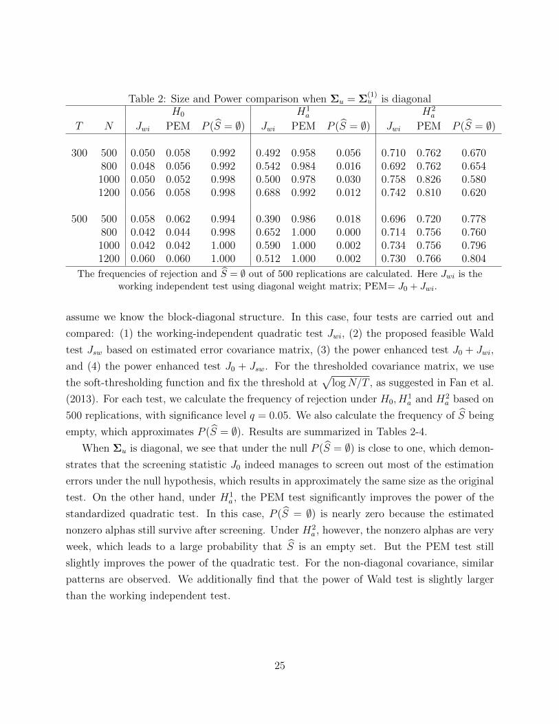
Table 2: Size and Power comparison when Σu = Σ(1)u is diagonal

H0 H1a H2

a

T N Jwi PEM P (S = ∅) Jwi PEM P (S = ∅) Jwi PEM P (S = ∅)

300 500 0.050 0.058 0.992 0.492 0.958 0.056 0.710 0.762 0.670800 0.048 0.056 0.992 0.542 0.984 0.016 0.692 0.762 0.6541000 0.050 0.052 0.998 0.500 0.978 0.030 0.758 0.826 0.5801200 0.056 0.058 0.998 0.688 0.992 0.012 0.742 0.810 0.620

500 500 0.058 0.062 0.994 0.390 0.986 0.018 0.696 0.720 0.778800 0.042 0.044 0.998 0.652 1.000 0.000 0.714 0.756 0.7601000 0.042 0.042 1.000 0.590 1.000 0.002 0.734 0.756 0.7961200 0.060 0.060 1.000 0.512 1.000 0.002 0.730 0.766 0.804

The frequencies of rejection and S = ∅ out of 500 replications are calculated. Here Jwi is theworking independent test using diagonal weight matrix; PEM= J0 + Jwi.

assume we know the block-diagonal structure. In this case, four tests are carried out and

compared: (1) the working-independent quadratic test Jwi, (2) the proposed feasible Wald

test Jsw based on estimated error covariance matrix, (3) the power enhanced test J0 + Jwi,

and (4) the power enhanced test J0 + Jsw. For the thresholded covariance matrix, we use

the soft-thresholding function and fix the threshold at√

logN/T , as suggested in Fan et al.

(2013). For each test, we calculate the frequency of rejection under H0, H1a and H2

a based on

500 replications, with significance level q = 0.05. We also calculate the frequency of S being

empty, which approximates P (S = ∅). Results are summarized in Tables 2-4.

When Σu is diagonal, we see that under the null P (S = ∅) is close to one, which demon-

strates that the screening statistic J0 indeed manages to screen out most of the estimation

errors under the null hypothesis, which results in approximately the same size as the original

test. On the other hand, under H1a , the PEM test significantly improves the power of the

standardized quadratic test. In this case, P (S = ∅) is nearly zero because the estimated

nonzero alphas still survive after screening. Under H2a , however, the nonzero alphas are very

week, which leads to a large probability that S is an empty set. But the PEM test still

slightly improves the power of the quadratic test. For the non-diagonal covariance, similar

patterns are observed. We additionally find that the power of Wald test is slightly larger

than the working independent test.

25

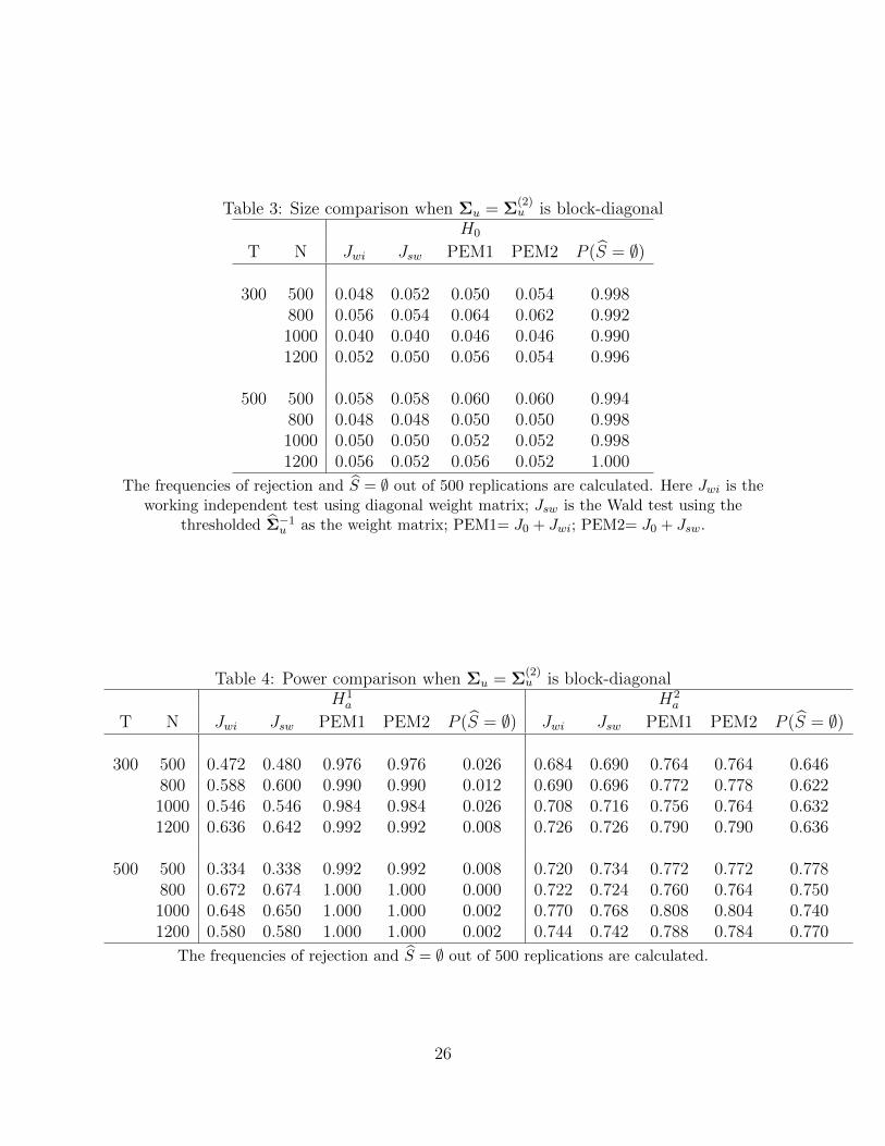
Table 3: Size comparison when Σu = Σ(2)u is block-diagonal

H0

T N Jwi Jsw PEM1 PEM2 P (S = ∅)

300 500 0.048 0.052 0.050 0.054 0.998800 0.056 0.054 0.064 0.062 0.9921000 0.040 0.040 0.046 0.046 0.9901200 0.052 0.050 0.056 0.054 0.996

500 500 0.058 0.058 0.060 0.060 0.994800 0.048 0.048 0.050 0.050 0.9981000 0.050 0.050 0.052 0.052 0.9981200 0.056 0.052 0.056 0.052 1.000

The frequencies of rejection and S = ∅ out of 500 replications are calculated. Here Jwi is theworking independent test using diagonal weight matrix; Jsw is the Wald test using the

thresholded Σ−1u as the weight matrix; PEM1= J0 + Jwi; PEM2= J0 + Jsw.

Table 4: Power comparison when Σu = Σ(2)u is block-diagonal

H1a H2

a

T N Jwi Jsw PEM1 PEM2 P (S = ∅) Jwi Jsw PEM1 PEM2 P (S = ∅)

300 500 0.472 0.480 0.976 0.976 0.026 0.684 0.690 0.764 0.764 0.646800 0.588 0.600 0.990 0.990 0.012 0.690 0.696 0.772 0.778 0.6221000 0.546 0.546 0.984 0.984 0.026 0.708 0.716 0.756 0.764 0.6321200 0.636 0.642 0.992 0.992 0.008 0.726 0.726 0.790 0.790 0.636

500 500 0.334 0.338 0.992 0.992 0.008 0.720 0.734 0.772 0.772 0.778800 0.672 0.674 1.000 1.000 0.000 0.722 0.724 0.760 0.764 0.7501000 0.648 0.650 1.000 1.000 0.002 0.770 0.768 0.808 0.804 0.7401200 0.580 0.580 1.000 1.000 0.002 0.744 0.742 0.788 0.784 0.770

The frequencies of rejection and S = ∅ out of 500 replications are calculated.

26

8 Empirical Study

We apply the proposed thresholded Wald test and the PEM to the securities in the S&P

500 index, by employing the Fama-French three-factor (FF-3) model to conduct our test.

One of our empirical findings is that market inefficiency is primarily caused by a small portion

of stocks with positive alphas, instead of a large portion of slightly mispriced assets. This

provides empirical evidence of sparse alternatives. In addition, the market inefficiency is

further evidenced by our newly created portfolio based on the PEM test, which outperforms

the SP500 index.

We collect monthly returns on all the S&P 500 constituents from the CRSP database

for the period January 1980 to December 2012, during which a total of 1170 stocks have

entered the index for our study. Testing of market efficiency is performed on a rolling window

basis: for each month from December 1984 to December 2012, we evaluate our test statistics

using the preceding 60 months’ returns (T = 60). The panel at each testing month consists

of stocks without missing observations in the past five years, which yields a cross-sectional

dimension much larger than the time-series dimension (N > T ). In this manner we not

only capture the up-to-date information in the market, but also mitigate the impact of

time-varying factor loadings. For testing months τ = 12/1984, ..., 12/2012, we run the FF-3

regressions

rτit − rτft = ατi + βτi,MKT(MKTτt − rτft) + βτi,SMBSMBτ

t + βτi,HMLHMLτt + uτit, (8.1)

for i = 1, ..., Nτ and t = τ − 59, ..., τ , where rit represents the return for stock i at month t,

rft the risk free rate, and MKT, SMB and HML constitute the FF-3 model’s market, size and

value factors. Our null hypothesis ατi = 0 for all i implies that the market is mean-variance

efficient.

Table 5: Variable descriptive statistics for the FF-3 modelVariables Mean Std dev. Median Min MaxNτ 617.70 26.31 621 574 665

|S|0 5.49 5.48 4 0 37

|α|τ

i (%) 0.9973 0.1630 0.9322 0.7899 1.3897

|α|τ

i∈S(%) 4.3003 0.9274 4.1056 1.7303 8.1299p-value of Jwi 0.2844 0.2998 0.1811 0 0.9946p-value of Jsw 0.1861 0.2947 0.0150 0 0.9926p-value of PEM 0.1256 0.2602 0.0003 0 0.9836

27

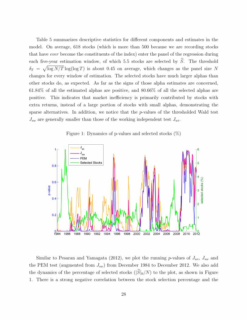
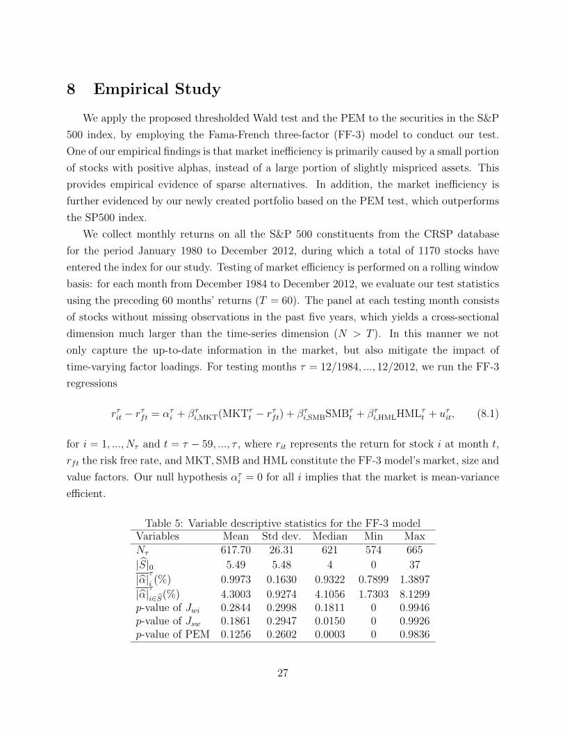
Table 5 summarizes descriptive statistics for different components and estimates in the

model. On average, 618 stocks (which is more than 500 because we are recording stocks

that have ever become the constituents of the index) enter the panel of the regression during

each five-year estimation window, of which 5.5 stocks are selected by S. The threshold

δT =√

logN/T log(log T ) is about 0.45 on average, which changes as the panel size N

changes for every window of estimation. The selected stocks have much larger alphas than

other stocks do, as expected. As far as the signs of those alpha estimates are concerned,

61.84% of all the estimated alphas are positive, and 80.66% of all the selected alphas are

positive. This indicates that market inefficiency is primarily contributed by stocks with

extra returns, instead of a large portion of stocks with small alphas, demonstrating the

sparse alternatives. In addition, we notice that the p-values of the thresholded Wald test

Jsw are generally smaller than those of the working independent test Jwi.

Figure 1: Dynamics of p-values and selected stocks (%)

Similar to Pesaran and Yamagata (2012), we plot the running p-values of Jwi, Jsw and

the PEM test (augmented from Jsw) from December 1984 to December 2012. We also add

the dynamics of the percentage of selected stocks (|S|0/N) to the plot, as shown in Figure

1. There is a strong negative correlation between the stock selection percentage and the

28

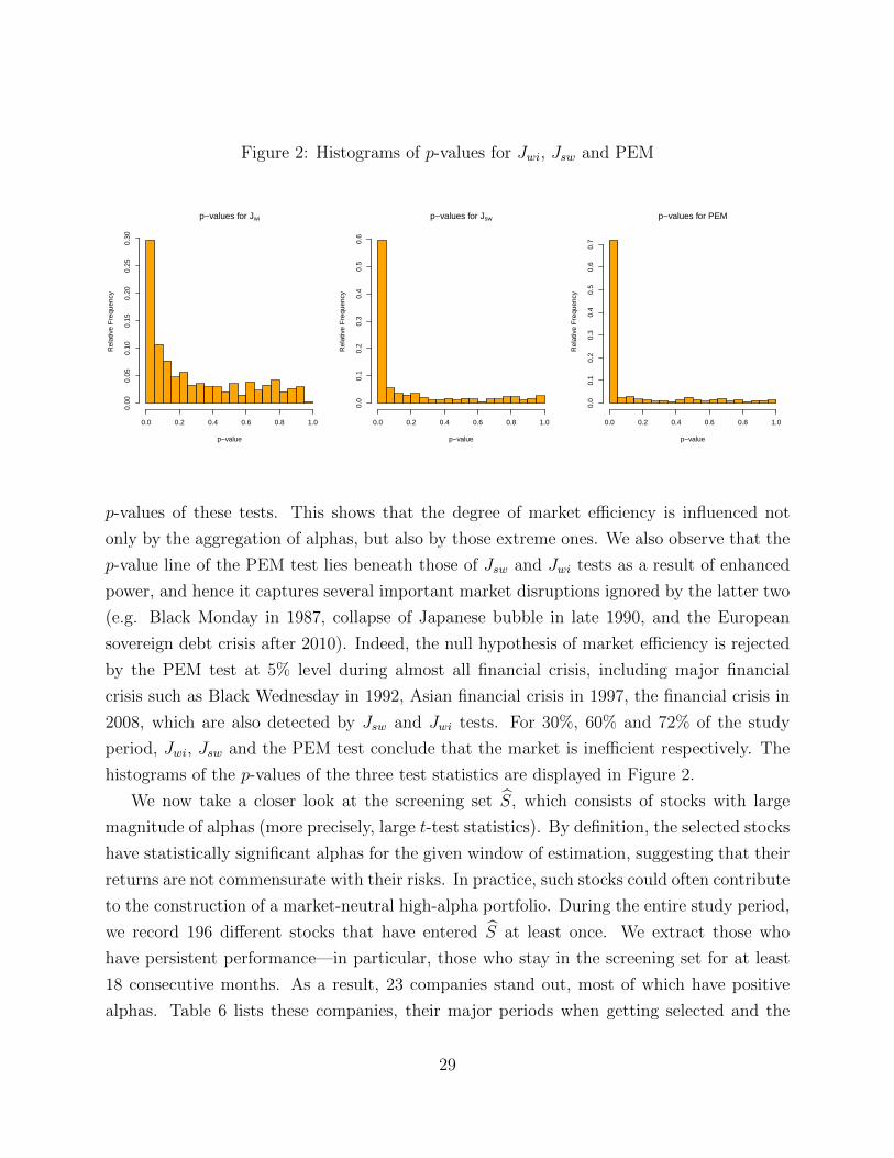
Figure 2: Histograms of p-values for Jwi, Jsw and PEM

p−values for Jwi

p−value

Rel

ativ

e F

requ

ency

0.0 0.2 0.4 0.6 0.8 1.0

0.00

0.05

0.10

0.15

0.20

0.25

0.30

p−values for Jsw

p−value

Rel

ativ

e F

requ

ency

0.0 0.2 0.4 0.6 0.8 1.0

0.0

0.1

0.2

0.3

0.4

0.5

0.6

p−values for PEM

p−value

Rel

ativ

e F

requ

ency

0.0 0.2 0.4 0.6 0.8 1.0

0.0

0.1

0.2

0.3

0.4

0.5

0.6

0.7

p-values of these tests. This shows that the degree of market efficiency is influenced not

only by the aggregation of alphas, but also by those extreme ones. We also observe that the

p-value line of the PEM test lies beneath those of Jsw and Jwi tests as a result of enhanced

power, and hence it captures several important market disruptions ignored by the latter two

(e.g. Black Monday in 1987, collapse of Japanese bubble in late 1990, and the European

sovereign debt crisis after 2010). Indeed, the null hypothesis of market efficiency is rejected

by the PEM test at 5% level during almost all financial crisis, including major financial

crisis such as Black Wednesday in 1992, Asian financial crisis in 1997, the financial crisis in

2008, which are also detected by Jsw and Jwi tests. For 30%, 60% and 72% of the study

period, Jwi, Jsw and the PEM test conclude that the market is inefficient respectively. The

histograms of the p-values of the three test statistics are displayed in Figure 2.

We now take a closer look at the screening set S, which consists of stocks with large

magnitude of alphas (more precisely, large t-test statistics). By definition, the selected stocks

have statistically significant alphas for the given window of estimation, suggesting that their

returns are not commensurate with their risks. In practice, such stocks could often contribute

to the construction of a market-neutral high-alpha portfolio. During the entire study period,

we record 196 different stocks that have entered S at least once. We extract those who

have persistent performance—in particular, those who stay in the screening set for at least

18 consecutive months. As a result, 23 companies stand out, most of which have positive

alphas. Table 6 lists these companies, their major periods when getting selected and the

29

associated alphas. We observe that companies such as Walmart, Dell and Apple exhibited

large positive alphas during their periods of rapid growth, whereas some others like Massey

Energy experienced very low alphas at their stressful times.

Table 6: Companies with longest selection periodCompany Name Major period of selection Average alpha (%) Std. dev. (%)T J X COMPANIES INC NEW 12/1984—08/1986 3.8230 0.2055HASBRO INDUSTRIES INC * 12/1984—03/1987 5.7285 0.5362WAL MART STORES INC * 12/1984—03/1987 2.7556 0.1672MASSEY ENERGY CO 10/1985—03/1987 -3.7179 0.2778DEERE & CO 11/1985—04/1987 -3.0385 0.3328CIRCUIT CITY STORES INC 11/1985—09/1987 6.4062 0.7272CLAIBORNE INC 06/1986—04/1988 4.1017 0.8491ST JUDE MEDICAL INC * 10/1989—09/1991 4.1412 0.3794HOME DEPOT INC *** 08/1990—01/1995 3.4988 0.4887UNITED STATES SURGICAL CORP * 11/1990—03/1993 4.2471 0.4648INTERNATIONAL GAME TECHNOLOGY 02/1992—11/1993 5.4924 0.4993UNITED HEALTHCARE CORP ** 07/1992—04/1995 4.9666 0.3526H B O & CO *** 10/1995—09/1998 4.9303 0.6193SAFEWAY INC 08/1997—04/1999 3.8200 0.3709CISCO SYSTEMS INC *** 10/1997—12/2000 3.8962 0.3352DELL COMPUTER CORP 04/1998—10/1999 7.5257 0.7335SUN MICROSYSTEMS INC 01/1999—11/2000 4.6975 0.2630J D S UNIPHASE CORP * 01/1999—05/2001 6.9504 0.5183HANSEN NATURAL CORP * 11/2005—10/2007 8.1486 0.5192CELGENE CORP 04/2006—11/2007 5.4475 0.4210MONSANTO CO NEW 09/2007—05/2009 3.5641 0.3462GANNETT INC 10/2007—03/2009 -2.7909 0.7952APPLE COMPUTER INC 03/2008—10/2009 4.8959 0.3740

Major period of selection refers to the time interval of at least 18 months when those companies stay in thescreening set. The average and standard deviations of the alphas are computed during the period of

selection. We mark companies that stand out for at least 24 months by ∗ (30 months by ∗∗ and 36 monthsby ∗ ∗ ∗ respectively).

Our test also has a number of implications in terms of portfolio construction. In fact,

a simple trading strategy can be designed based on the obtained screening set. At the

beginning of month t, we run regressions (8.1) over a 60-month period from month t− 60 to

month t− 1. From the estimated screening set S we extract stocks that have positive alphas

and construct a equal-weighted long-only portfolio. The portfolio is held for a one-month

period and rebalanced at the beginning of month t + 1. For diversification purposes, if S

contains less than 2 stocks, we invest all the money into the S&P 500 index. Transaction

costs are ignored here.

Figure 3 compares our trading strategy with the S&P 500 index from January 1985

to December 2012. The top panel gives the excess return of the equal-weighted long-only

30

Figure 3: Monthly excess returns (top panel, returns of the new trading strategy subtractingS&P500 index) and cumulative total returns (bottom panel) of the long-only portfolio relativeto the S&P 500

31

portfolio over the S&P 500 index during each month. The monthly excess return has a

mean of 0.9%, and in particular, for 202 out of the 336 study months, our strategy generates

a higher return than the S&P 500. The cumulative performance of the two portfolios is

depicted in the bottom panel. Our long-only portfolio has a monthly mean return of 1.64%

and a standard deviation of 7.48% during the period, whereas those for the S&P 500 are

0.74% and 4.48% respectively. The monthly Sharpe ratio for our strategy is 0.1759, and

the Sharpe ratio for the S&P 500 is 0.0936. They are equivalent to an annual Sharpe ratio

of 0.6093 and 0.3242 (multiplied by√

12). Our strategy clearly outperforms the S&P 500

over the sample period with a higher Sharpe ratio. This is because the degree of market

efficiency is dynamic and it often takes time for market participants to adapt to changing

market conditions. Arbitrage opportunities as indicated by large positive alphas are not

competed away immediately. By holding stocks with large positive alphas for a one-month

period, we are likely to get higher returns without bearing as much risk.

9 Concluding remarks

The literature on testing mean-variance efficiency is predominated by low-dimensional

tests based on constructed portfolios, which test only one part of the pricing theory and

are subject to selection and unintentional biases. Recent efforts of extending them to high-

dimensional tests are only able to detect market inefficiency in an average sense as measured

by the weighted quadratic form α′Vα. However, when we deal with large panels, it is

more appealing if we could identify individual departures from the factor pricing model, and

handle the case when there are small portions of large alphas.

We propose a new concept for high dimensional statistical tests, namely, the power en-

hancement (PEM). The PEM test combines a PEM component and a Wald-type statistic.

Under the null hypothesis, the PEM component equals zero with probability approach-

ing one, whereas under the alternative hypothesis it is stochastically unbounded over some

high-power regions. Hence while maintaining a good size asymptotically, the PEM test sig-

nificantly enhances the power of Wald-type statistics. As a by-product, the selected subset

S also enables us to identify those significant alphas. Furthermore, the PEM technique

is potentially widely applicable in many high-dimensional testing problems in panel data

analysis, such as testing the cross-sectional independence and over-identifying constraints.

We also develop a high-dimensional Wald test when the covariance matrix of idiosyn-

cratic noises is sparse, using the thresholded sample covariance matrix of the idiosyncratic

32

components. We develop new techniques to prove that the effect of estimating the inverse

covariance matrix is asymptotically negligible. Therefore, the aggregation of estimation er-

rors is successfully avoided. This technique is potentially useful in other high-dimensional

econometric applications, where an optimal weight matrix needs to be estimated, such as

GMM and GLS.

Our empirical study shows that the market inefficiency is primarily caused by a small

portion of significantly mis-priced stocks, instead of a large portion of slightly mis-priced

stocks. In addition, most of the selected stocks have positive alphas. The market inefficiency

is further evidenced by our newly created portfolio based on the PEM test, which outperforms

the S&P500 index.

APPENDIX

A Proofs

We first cite a lemma that will be needed throughout the proofs. Write σij = (Σu)ij and

σij = 1T

∑Tt=1 uitujt. Recall σ2

j = (Σu)jj/(1− Ef ′t(Eftf′t)−1Eft), and σ2

j = σjj/(1− f ′w).

Lemma A.1. Under Assumption 3.2, there is C > 0,

(i) P (maxi,j≤N | 1T∑T

t=1 uitujt − Euitujt| > C√

logNT

)→ 0.

(ii) P (maxi≤K,j≤N | 1T∑T

t=1 fitujt| > C√

logNT

)→ 0.

(iii) P (maxj≤N | 1T∑T

t=1 ujt| > C√

logNT

)→ 0.

Proof. The proof follows from Lemmas A.3 and B.1 in Fan, Liao and Mincheva (2011).

Lemma A.2. When the distribution of (ut, ft) is independent of α, under Assumption 3.2,

there is C > 0,

(i) supα∈RN P (maxj≤N |αj − αj| > C√

logNT|α)→ 0

(ii) supα∈RN P (maxi,j≤N |σij − σij| > C√

logNT|α)→ 0,

(iii) supα∈RN P (maxi≤N |σi − σi| > C√

logNT|α)→ 0.

Proof. Note that αj−αj = 1τT

∑Tt=1 ujt(1−f ′tw). Here τ = 1− f ′w→p 1−Ef ′t(Eftf

′t)−1Eft >

0, hence τ is bounded away from zero with probability approaching one. Thus by Lemma

A.1, there is C > 0 independent of α, such that

supα∈RN

P (maxj≤N|αj − αj| > C

√logN

T|α) = P (max

j| 1

τT

T∑t=1

ujt(1− f ′tw)| > C

√logN

T)→ 0

33

(ii) There is C independent of α, such that the event

A = maxi,j| 1T

T∑t=1

uitujt − σij| < C

√logN

T,

1

T

T∑t=1

‖ft‖2 < C

has probability approaching one. Also, there is C2 also independent of α such that the event

B = maxi1T

∑t u

2it < C2 occurs with probability approaching one. Then on the event

A ∩B, by the triangular and Cauchy-Schwarz inequalities,

|σij − σij| ≤ C

√logN

T+ 2 max

i

√1

T

∑t

(uit − uit)2C2 + maxi

1

T

∑t

(uit − uit)2.

It can be shown that

maxi≤N

1

T

T∑t=1

(uit − uit)2 ≤ maxi

(‖bi − bi‖2 + (αi − αi)2)(1

T

T∑t=1

‖ft‖2 + 1).

Note that bi−bi and αi−αi only depend on (ft,ut). By Lemma 3.1 of Fan et al. (2011), there

is C3 > 0 such that supb,α P (maxi≤N ‖bi − bi‖2 + (αi − αi)2 > C3logNT

) = o(1). Combining

the last two displayed inequalities yields, for C4 = (C + 1)C3,

supαP (max

i≤N

1

T

T∑t=1

(uit − uit)2 > C4logN

T|α) = o(1),

which yields the desired result.

(iii): Recall σ2j = σjj/τ , and σ2

j = σjj/(1−Ef ′t(Eftf′t)−1Eft). Moreover, τ is independent

of α. The result follows immediately from part (ii).

Lemma A.3. For any ε > 0, supα P (‖Σ−1u −Σ−1

u ‖ > ε|α) = o(1).

Proof. By Lemma A.2 (ii), supα∈RN P (maxi,j≤N |σij − σij| > C√

logNT|α)→ 1. By Theorem

A.1 of Fan et al. (2013), on the event maxi,j≤N |σij − σij| ≤ C√

logNT

, there is constant C ′

that is independent of α,

‖Σ−1u −Σ−1

u ‖ ≤ C ′mN(logN

T)(1−k)/2.

Hence the result follows due to the sparse condition mN( logNT

)(1−k)/2 = o(1).

34

A.1 Proof of Theorem 2.1

Without loss of generality, under the alternative, let α′ = (α′1,α′2) = (0′,α′2), where

dim(α1) = N − r and dim(α2) = r. Correponding to (α′1,α′2), we partition Σu and Σ−1

u

into:

Σu =

(Σ1 β′

β Σ2

), Σ−1

u =

(Σ−1

1 + A G′

G C

).

By the matrix inversion formula, A = Σ−11 β′(Σ2 − βΣ−1

1 β′)−1βΣ−11 . We also partition the

estimator into α′ = (α′1, α′2). Note that α′Σ−1

u α = α′1Σ−11 α1 +α′1Aα1 +2α′2Gα1 +α′2Cα2.

We first look at α′1Aα1. Write ξ = Σ−11 α1, whose ith element is denoted by ξi. It follows

from ‖Σ−11 ‖1 <∞ that

maxi≤N−r

|ξi| = OP ( maxi≤N−r

|α1i|) = OP ( maxi≤N−r

|α1i − α1i|) = OP (

√logN

T).

Also, maxi≤r∑N−r

j=1 |βij| ≤ ‖Σu‖1 = O(1), and λmax((Σ2 − βΣ−11 β′)−1) = O(1). Hence

|α′1Aα1| = O(1)‖βξ‖2 ≤ O(1) maxj|ξj|2

r∑i=1

(N−r∑j=1

|βij|)2 = OP (r logN

T).

For G = (gij), note that maxi≤r∑N−r

j=1 |gij| ≤ ‖Σ−1u ‖1 = O(1). Hence

|α′2Gα1| ≤ maxj≤N−r

|α1j|maxj≤r|α2j|

r∑i=1

N−r∑j=1

|gij| ≤ OP (r

√logN

T)

where we used the fact that maxj≤r |α2j| ≤ maxj |α2j| + maxj |αj − αj| = OP (1). Also,

|α′2Cα2| ≤ ‖α2‖2‖C‖ = OP (r). It then yields, under Ha,

κ = α′Σ−1u α− α′1Σ

−11 α1 = OP (r).

It also follows from (2.2) that

Z ≡ aT α′1Σ−11 α1 − (N − r)√2(N − r)

→d N (0, 1).

As aT = Tτ = OP (T ), we have (aTκ− r/√

2)/√N = OP (Tr/

√N). Since Tr = o(

√N), for

35

any ε ∈ (0, zq), for all large N, T , the following event holds with probability at least 1− ε:

A = |aTκ− r/√

2| <√Nε.

Using 1−Φ(zq) = q and choosing ε small enough such that 1−Φ(zq − ε) + ε < 2q, we have,

P (J1 > zq) = P (aT (α′1Σ

−11 α1 + κ)−N√

2N> zq)

= P (Z

√N − rN

+aTκ− r/

√2√

N> zq)

≤ P (Z

√N − rN

+ ε > zq) + P (Ac)

≤ 1− Φ(zq − ε) + ε+ o(1),

which is bounded by 2q. This implies the result.

A.2 Proof of Theorem 3.1 and Corollary 3.1

(i) For any j ∈ S, by the definition of S,|αj |σj

> 2δT . Define events

A1 =

maxj≤N|σ−1j − σ−1

j | ≤ C2

, A2 =

maxj≤N|αj − αj| ≤ C3δT

for some C2, C3 > 0. Lemma A.2 then implies that infα P (A1 ∩ A2)→ 1. Under A1 ∩ A2,

|αj|σj

≥ (|αj| −maxj|αj − αj|)(σ−1

j −maxj|σ−1j − σ−1

j |)

≥ (|αj| − C3δT )(σ−1j − C2) ≥ δT ,

where the last inequality holds for sufficiently small C2, C3, e.g., C3 < minjσj2

and C2 =13

minj(σ−1j ). This implies that j ∈ S, hence P (S ⊂ S)→ 1. It can be readily seen that if j ∈

S, by similar arguments, we have|αj |σj

> 12δT with probability tending to one. Consequently,

S \S ⊂ G with probability approaching one. In fact we have proved infα P (S ⊂ S)→ 1 and

infα P (S \ S ⊂ G)→ 1.

(ii) Suppose minj≤N σj > C1 for some C1 > 0. For some constants C2 > 0 and C3 <

36

(C2 + C−11 )−1, under the event A1 ∩ A2 and H0, we have

maxj≤N

|αj|σj

≤ max |αj| ·maxj

(σ−1j ) ≤ C3δT · (max |σ−1

j − σ−1j |+ maxσ−1

j )

≤ C3(C2 + C−11 )δT ≤ δT ,

where we note that under H0, maxj |αj| = Op(√

logNT

). Hence P (maxj≤N|αj |σj≤ δT ) → 1,

which implies P (S = ∅)→ 1. This immediately implies P (J0 = 0)→ 1.

Corollary 3.1 is implied by part (i).

A.3 Proof of Theorem 3.2

Part (i) follows immediately from that P (J0 = 0|H0)→ 1.

(ii) Let Fq be the qth quantile of F , then under the level (1 − q). Then both J and J1

reject H0 if J0 ≥ Fq. Since J1 has high power uniformly on Ω1, it follows from J ≥ J1

infα∈Ω1

P (J ≥ Fq|α) ≥ infα∈Ω1

P (J1 ≥ Fq|α)→ 1,

which implies that J also has power uniformly on Ω1. We now show J also has high power

uniformly on

Ω0 = α ∈ RN : maxj≤N|αj| > 2δT max

j≤Nσj.

First of all, Ω0 ⊂ S. It follows from infα∈Ω0 P (S ⊂ S) → 1 that infα∈Ω0 P (S 6= ∅) → 1.

Lemma A.3 then implies λmin(Σ−1

S) is bounded away from zero with probability approaching

one. Under the event S ⊂ S, we have ‖αS‖ ≥ ‖αS‖. Hence there is a constant C > 0 so

that with probability approaching one (uniformly in α),

J0/√N ≥ CT‖αS‖

2 ≥ CT‖αS‖2 ≥ CT (‖αS‖ − ‖αS −αS‖)2.

On one hand, on Ω0, ‖αS‖2 ≥ minj∈S α2j |S|0 ≥ |S|0δ2

T4 minj σ2j . On the other hand, ∃C2 > 0,

by Lemma A.2(i),

supαP

(‖αS −αS‖2 >

C2 logN

T|S|0

∣∣α) = o(1).

Then for any α ∈ Ω0, because log(log T ) minj σj → ∞, as minj σj is bounded away from

37

zero,

‖αS‖−√C2 logN |S|0

T≥√|S|0 logN

T(log(log T )2 min

jσj−

√C2) ≥

√|S|0 logN

Tlog(log T ) min

jσj.

Hence uniformly on α ∈ Ω0,

P (J0/√N ≥ CT (‖αS‖ − ‖αS −αS‖)2

∣∣α) ≤ P (J0/√N ≥ CT (‖αS‖ −

√C2 logN |S|0

T)2∣∣α)

+ supαP (‖αS −αS‖2 >

C2 logN

T|S|0

∣∣α)

≤ P (J0/√N ≥ C|S|0 logN log2(log T ) min

jσ2j

∣∣α) + o(1),

where the term o(1) is uniform in α ∈ Ω0.

Because infα∈Ω0 P (J0/√N ≥ CT (‖αS‖−‖αS −αS‖)2

∣∣α)→ 1, and |S|0 ≥ 1 when there

is α ∈ Ω0, for gT ≡ C logN log2(log T ) minj σ2j →∞,

infα∈Ω0

P (J0 ≥√NgT

∣∣α)→ 1. (A.1)

Note that J1 is standardized such that Fq = O(1) uniformly in α, and there is c > 0,

infα∈Ω0 P (J1 ≥ −c√N |α)→ 1. Hence gT →∞ implies

infα∈Ω0

P (J > Fq|α) ≥ infα∈Ω0

P (√NgT − c

√N > Fq|α)− o(1) = 1− o(1).

This proves the uniform powerfulness of J on Ω0. Combining Ω0 and Ω1, we have

infα∈Ω1∪Ω0

P (J > Fq|α)→ 1.

A.4 Proof of Theorem 4.1

It follows from Pesaran and Yamagata (2012 Section 4.4) that Jwi → N (0, 1). For

Ω1 = ‖α‖2 N logN/T, by Lemma A.2,

infα∈Ω1

P (‖α‖2 ≥ N logN

4T

∣∣α)→ 1.

38

So infα∈Ω1 P (Jwi > C√N logN |α)→ 1 for some C > 0. It then follows from J ≥ Jwi that

infα∈Ω1

P (J ≥ C√N logN |α) ≥ inf

α∈Ω1

P (Jwi ≥ C√N logN |α)→ 1.

In addition, Jwi ≥ −√N/2. By (A.1), we have

infα∈Ω0

P (J ≥ aT√N/2|α) ≥ inf

α∈Ω0

P (J0 −√N/2 ≥ aT

√N/2|α)

≥ infα∈Ω0

P (J0 ≥√NaT |α)→ 1.

This implies that both infα∈Ω1 P (J > zq) and infα∈Ω0 P (J > zq) converge to one, which

yields infα∈Ω1∪Ω0 P (J > zq)→ 1.

A.5 Proof of Theorem 5.1

The proof of part (ii) is the same as that of Theorem 3.2. Moreover, it follows from

Pesaran and Yamagata (2012, Theorem 1) that (aT α′Σ−1

u α−N)/√

2N →d N (0, 1). So the

theorem is proved by Proposition A.1 below.

Proposition A.1. Under the assumptions of Theorem 5.1, and under H0,

T α′(Σ−1u − Σ−1

u )α√N

= oP (1)

Define et = Σ−1u ut = (e1t, ..., eNt)

′, which is an N -dimensional vector with mean zero and

covariance Σ−1u , whose entries are stochastically bounded. Let w = (Eftf

′t)−1Eft. A key step

of proving the above proposition is to establish the following two convergences:

1

TE| 1√

NT

N∑i=1

T∑t=1

(u2it − Eu2

it)(1√T

T∑s=1

eis(1− f ′sw))2|2 = o(1), (A.2)

1

TE| 1√

NT

∑i 6=j,(i,j)∈SU

T∑t=1

(uitujt−Euitujt)[1√T

T∑s=1

eis(1−f ′sw)][1√T

T∑k=1

ejk(1−f ′kw)]|2 = o(1),

(A.3)

where

SU = (i, j) : (Σu)ij 6= 0.

The sparsity condition assumes that most of the off-diagonal entries of Σu are outside of SU .

39

The above two convergences are weighted cross-sectional and serial double sums, where the

weights satisfy 1√T

∑Tt=1 eit(1 − f ′tw) = OP (1) for each i. The proofs of (A.2) and (A.3) are

given in Appendix A.6.

Proof of PropositionA.1

Proof. The left hand side is equal to

T α′Σ−1u (Σu −Σu)Σ

−1u α′√

N+T α′(Σ−1

u −Σ−1u )(Σu −Σu)Σ

−1u α′√

N≡ a+ b.

It was shown by Fan et al. (2011) that ‖Σu − Σu‖ = OP (mN

√logNT

) = ‖Σ−1u − Σ−1

u ‖. In

addition, ‖α‖2 = OP (N logN/T ). Hence b = OP (m2

N

√N(logN)2

T) = oP (1).

It suffices to show a = oP (1). We consider the hard-thresholding covariance estimator.

The proof for the generalized sparsity case as in Rothman et al. (2009) is very similar.

Let sij = 1T

∑Tt=1 uitujt and σij = (Σu)ij. Under hard-thresholding,

σij = (Σu)ij =

sii, if i = j,

sij, if i 6= j, |sij| > C(siisjjlogNT

)1/2

0, if i 6= j, |sij| ≤ C(siisjjlogNT

)1/2

(A.4)

Write (α′Σ−1u )i to denote the ith element of α′Σ−1

u , and ScU = (i, j) : (Σu)ij = 0. For

σij ≡ (Σu)ij and σij = (Σu)ij, we have

a =T√N

N∑i=1

(α′Σ−1u )2

i (σii − σii) +T√N

∑i 6=j,(i,j)∈SU

(α′Σ−1u )i(α

′Σ−1u )j(σij − σij)

+T√N

∑(i,j)∈Sc

U

(α′Σ−1u )i(α

′Σ−1u )j(σij − σij)

= a1 + a2 + a3

We first examine a3. Note that

a3 =T√N

∑(i,j)∈Sc

U

(α′Σ−1u )i(α

′Σ−1u )jσij ≤ max

i≤N|(α′Σ−1

u )i|2T√N

∑(i,j)∈Sc

U

|σij| ≡ a31.

40

We have,

P (a31 > T−1) ≤ P ( max(i,j)∈Sc

U

|σij| 6= 0) ≤ P ( max(i,j)∈Sc

U

|sij| > C(siisjjlogN

T)1/2).

Because sii is uniformly (across i) bounded away from zero with probability approaching

one, and max(i,j)∈ScU|sij| = OP (

√logNT

). Hence for any ε > 0, when C in the threshold is

large enough, P (a31 > T−1) < ε, this implies a31 = oP (1), and thus a3 = oP (1).

The proof is finished once we establish ai = oP (1) for i = 1, 2, which are given respectively

by the following lemmas.

Lemma A.4. Under H0, a1 = oP (1).

Proof. We have a1 = T√N

∑Ni=1(α′Σ−1

u )2i

1T

∑Tt=1(u2

it − Eu2it), which is

T√N

N∑i=1

(α′Σ−1u )2

i

1

T

T∑t=1

(u2it − u2

it) +T√N

N∑i=1

(α′Σ−1u )2

i

1

T

T∑t=1

(u2it − Eu2

it) = a11 + a12.

For a12, note that (α′Σ−1u )i = (1− f ′w)−1 1

T

∑Ts=1(1− f ′sw)(u′sΣ

−1u )i = c 1

T

∑Ts=1(1− f ′sw)eis,

where c = (1− f ′w)−1 = OP (1). Hence

a12 =Tc√N

N∑i=1

(1

T

T∑s=1

(1− f ′sw)eis)2 1

T

T∑t=1

(u2it − Eu2

it)

By (A.2) (whose proof is given in Appendix A.6), Ea212 = o(1). On the other hand,

a11 =T√N

N∑i=1

(α′Σ−1u )2

i

1

T

T∑t=1

(uit−uit)2 +2T√N

N∑i=1

(α′Σ−1u )2

i

1

T

T∑t=1

uit(uit−uit) = a111 +a112.

Note that maxi≤N1T

∑Tt=1(uit − uit)2 = OP ( logN

T) by Lemma 3.1 of Fan et al. (2011). Since

‖α‖2 = OP (N logNT

), ‖Σ−1u ‖ = O(1) and N(logN)3 = o(T 2),

a111 ≤ OP (logN

T)T√N‖α′Σ−1

u ‖2 = OP ((logN)2

√N

T) = oP (1),

41

To bound a112, note that

uit − uit = αi − αi + (bi − bi)′ft, max

i‖αi − αi‖ = OP (

√logN

T) = max

i‖bi − bi‖.

Also, maxi | 1T∑T

t=1 uit| = OP (√

logNT

) = maxi ‖ 1T

∑Tt=1 uitft‖. Hence

a112 =2T√N

N∑i=1

(α′Σ−1u )2

i

1

T

T∑t=1

uit(αi − αi) +2T√N

N∑i=1

(α′Σ−1u )2

i (bi − bi)′ 1

T

T∑t=1

ftuit

≤ OP (logN√N

)‖α′Σ−1u ‖2 = oP (1).

In summary, a1 = a12 + a111 + a112 = oP (1).

Lemma A.5. Under H0, a2 = oP (1).

Proof. We have a2 = T√N

∑i 6=j,(i,j)∈SU

(α′Σ−1u )i(α

′Σ−1u )j

1T

∑Tt=1(uitujt − Euitujt), which is

T√N

∑i 6=j,(i,j)∈SU

(α′Σ−1u )i(α

′Σ−1u )j

(1

T

T∑t=1

(uitujt − uitujt) +1

T

T∑t=1

(uitujt − Euitujt)

)= a21+a22.

where

a21 =T√N

∑i 6=j,(i,j)∈SU

(α′Σ−1u )i(α

′Σ−1u )j

1

T

T∑t=1

(uitujt − uitujt).

Under H0, Σ−1u α = 1

T(1− f ′w)−1

∑Tt=1 Σ−1

u ut(1− f ′tw), and et = Σ−1u ut, we have

a22 =T√N

∑i 6=j,(i,j)∈SU

(α′Σ−1u )i(α

′Σ−1u )j

1

T

T∑t=1

(uitujt − Euitujt)

=Tc√N

∑i 6=j,(i,j)∈SU

1

T

T∑s=1

(1− f ′sw)eis1

T

T∑k=1

(1− f ′kw)ejk1

T

T∑t=1

(uitujt − Euitujt).

By (A.3) (whose proof is given in Appendix A.6), Ea222 = o(1).

On the other hand, a21 = a211 + a212, where

a211 =T√N

∑i 6=j,(i,j)∈SU

(α′Σ−1u )i(α

′Σ−1u )j

1

T

T∑t=1

(uit − uit)(ujt − ujt),

42

a212 =2T√N

∑i 6=j,(i,j)∈SU

(α′Σ−1u )i(α

′Σ−1u )j

1

T

T∑t=1

uit(ujt − ujt).

By the Cauchy-Schwarz inequality, maxij | 1T∑T

t=1(uit − uit)(ujt − ujt)| = OP ( logNT

). Hence

|a211| ≤ OP (logN√N

)∑

i 6=j,(i,j)∈SU

|(α′Σ−1u )i||(α′Σ−1

u )j|

≤ OP (logN√N

)

∑i 6=j,(i,j)∈SU

(α′Σ−1u )2

i

1/2 ∑i 6=j,(i,j)∈SU

(α′Σ−1u )2

j

1/2

= OP (logN√N

)N∑i=1

(α′Σ−1u )2

i

∑j:(Σu)ij 6=0

1 ≤ OP (logN√N

)‖α′Σ−1u ‖2mN

= OP (mN

√N(logN)2

T) = oP (1).

Similar to the proof of term a112 in Lemma A.4, maxij | 1T∑T

t=1 uit(ujt−ujt)| = OP ( logNT

).

|a212| ≤ OP (logN√N

)∑

i 6=j,(i,j)∈SU

|(α′Σ−1u )i||(α′Σ−1

u )j| = OP (mN

√N(logN)2

T) = oP (1).

In summary, a2 = a22 + a211 + a212 = oP (1).

A.6 Proof of (A.2) and (A.3)

For any index set A, we let |A|0 denote its number of elements.

Lemma A.6. Recall that et = Σ−1u ut. eit and ujt are independent if i 6= j.

Proof. Because ut is Gaussian, it suffices to show that cov(eit, ujt) = 0 when i 6= j. Consider

the vector (u′t, e′t)′ = A(u′t,u

′t)′, where

A =

(IN 0

0 Σ−1u

).

Then cov(u′t, e′t) = Acov(u′t,u

′t)A, which is(

IN 0

0 Σ−1u

)(Σu Σu

Σu Σu

)(IN 0

0 Σ−1u

)=

(Σu IN

IN Σ−1u

).

43

This completes the proof.

A.6.1 Proof of (A.2)

Let X = 1√NT

∑Ni=1

∑Tt=1(u2

it−Eu2it)(

1√T

∑Ts=1 eis(1− f ′sw))2. The goal is to show EX2 =

o(T ). We show respectively 1T

(EX)2 = o(1) and 1T

var(X) = o(1). The proof of (A.2) is the

same regardless of the type of sparsity in Assumption 5.2. For notational simplicity, let

ξit = u2it − Eu2

it, ζis = eis(1− f ′sw).

Then X = 1√NT

∑Ni=1

∑Tt=1 ξit(

1√T

∑Ts=1 ζis)

2. Because of the serial independence, ξit is

independent of ζjs if t 6= s, for any i, j ≤ N , which implies cov(ξit, ζisζik) = 0 as long as

either s 6= t or k 6= t.

Expectation

For the expectation,

EX =1√NT

N∑i=1

T∑t=1

cov(ξit, (1√T

T∑s=1

ζis)2) =

1

T√NT

N∑i=1

T∑t=1

T∑s=1

T∑k=1

cov(ξit, ζisζik)

=1

T√NT

N∑i=1

T∑t=1

(cov(ξit, ζ2it) + 2

∑k 6=t

cov(ξit, ζitζik))

=1

T√NT

N∑i=1

T∑t=1

cov(ξit, ζ2it) = O(

√N

T),

where the second last equality follows since Eξit = Eζit = 0 and when k 6= t cov(ξit, ζitζik) =

Eξitζitζik = EξitζitEζik = 0. It then follows that 1T

(EX)2 = O( NT 2 ) = o(1), given N = o(T 2).

Variance

Consider the variance. We have,

var(X) =1

N

N∑i=1

var(1√T

T∑t=1

ξit(1√T

T∑s=1

ζis)2)

+1

NT 3

∑i 6=j

∑t,s,k,l,v,p≤T

cov(ξitζisζik, ξjlζjvζjp) = B1 +B2.

44

B1 can be bounded by the Cauchy-Schwarz inequality. Note that Eξit = Eζjs = 0,

B1 ≤1

N

N∑i=1

E(1√T

T∑t=1

ξit(1√T

T∑s=1

ζis)2)2 ≤ 1

N

N∑i=1

[E(1√T

T∑t=1

ξit)4]1/2[E(

1√T

T∑s=1

ζis)8]1/2.

Hence B1 = O(1).

We now show 1TB2 = o(1). Once this is done, it implies 1

Tvar(X) = o(1). The proof of

(A.2) is then completed because 1TEX2 = 1

T(EX)2 + 1

Tvar(X) = o(1).

For two variables X, Y , writing X ⊥ Y if they are independent. Note that Eξit =

Eζis = 0, and when t 6= s, ξit ⊥ ζjs, ξit ⊥ ξjs, ζit ⊥ ζjs for any i, j ≤ N . Therefore, it

is straightforward to verify that if the set t, s, k, l, v, p contains more than three distinct

elements, then cov(ξitζisζik, ξjlζjvζjp) = 0. Hence if we denote Ξ as the set of (t, s, k, l, v, p)

such that t, s, k, l, v, p contains no more than three distinct elements, then its cardinality

satisfies: |Ξ|0 ≤ CT 3 for some C > 1, and∑t,s,k,l,v,p≤T

cov(ξitζisζik, ξjlζjvζjp) =∑

(t,s,k,l,v,p)∈Ξ

cov(ξitζisζik, ξjlζjvζjp).

Hence

B2 =1

NT 3

∑i 6=j

∑(t,s,k,l,v,p)∈Ξ

cov(ξitζisζik, ξjlζjvζjp).

Let us partition Ξ into Ξ1∪Ξ2 where each element (t, s, k, l, v, p) in Ξ1 contains exactly three

distinct indices, while each element in Ξ2 contains less than three distinct indices. We know

that 1NT 3

∑i 6=j∑

(t,s,k,l,v,p)∈Ξ2cov(ξitζisζik, ξjlζjvζjp) = O( 1

NT 3N2T 2) = O(N

T), which implies

1

TB2 =

1

NT 4

∑i 6=j

∑(t,s,k,l,v,p)∈Ξ1

cov(ξitζisζik, ξjlζjvζjp) +OP (N

T 2).

The first term on the right hand side can be written as∑5

h=1B2h. Each of these five terms

is defined and analyzed separately as below.

B21 =1

NT 4

∑i 6=j

T∑t=1

∑s 6=t

∑l 6=s,t

EξitξjtEζ2isEζ

2jl ≤ O(

1

NT)∑i 6=j

|Eξitξjt|.

Note that if (Σu)ij = 0, uit and ujt are independent, and hence Eξitξjt = 0. This implies

45

∑i 6=j |Eξitξjt| ≤ O(1)

∑i 6=j,(i,j)∈SU

1 = O(N). Hence B21 = o(1).

B22 =1

NT 4

∑i 6=j

T∑t=1

∑s 6=t

∑l 6=s,t

EξitζitEζisξjsEζ2jl.

By Lemma A.6, ujs and eis are independent for i 6= j. Also, ujs and fs are independent,

which implies ξjs and ζis are independent. So Eξjsζis = 0. It follows that B22 = 0.

B23 =1

NT 4

∑i 6=j

T∑t=1

∑s 6=t

∑l 6=s,t

EξitζitEζisζjsEξjlζjl = O(1

NT)∑i 6=j

|Eζisζjs|

= O(1

NT)∑i 6=j

|EeisejsE(1− f ′sw)2| = O(1

NT)∑i 6=j

|Eeisejs|.

By the definition es = Σ−1u us, cov(es) = Σ−1

u . Hence Eeisejs = (Σ−1u )ij, which implies

B23 ≤ O( NNT

)‖Σ−1u ‖1 = o(1).

B24 =1

NT 4

∑i 6=j

T∑t=1

∑s 6=t

∑l 6=s,t

EξitξjtEζisζjsEζilζjl = O(1

T),

which is analyzed in the same way as B21.

Finally, B25 = 1NT 4

∑i 6=j∑T

t=1

∑s 6=t∑

l 6=s,tEξitζjtEζisξjsEζilζjl = 0, because Eζisξjs = 0

when i 6= j, following from Lemma A.6. Therefore, 1TB2 = o(1) +O( N

T 2 ) = o(1).

A.6.2 Proof of (A.3)

For notational simplicity, let ξijt = uitujt − Euitujt. Because of the serial independence

and the Gaussianity, cov(ξijt, ζlsζnk) = 0 when either s 6= t or k 6= t, for any i, j, l, n ≤ N . In

addition, define a set

H = (i, j) ∈ SU : i 6= j.

Then by the sparsity assumption,∑

(i,j)∈H 1 = DN = O(N). Now let

Z =1√NT

∑(i,j)∈H

T∑t=1

(uitujt − Euitujt)[1√T

T∑s=1

eis(1− f ′sw)][1√T

T∑k=1

ejk(1− f ′kw)]

=1√NT

∑(i,j)∈H

T∑t=1

ξijt[1√T

T∑s=1

ζis][1√T

T∑k=1

ζjk] =1

T√NT

∑(i,j)∈H

T∑t=1

T∑s=1

T∑k=1

ξijtζisζjk.

46

The goal is to show 1TEZ2 = o(1). We respectively show 1

T(EZ)2 = o(1) = 1

Tvar(Z).

Expectation

The proof for the expectation is the same regardless of the type of sparsity in Assumption

5.2, and is very similar to that of (A.2). In fact,

EZ =1

T√NT

∑(i,j)∈H

T∑t=1

T∑s=1

T∑k=1

cov(ξijt, ζisζjk) =1

T√NT

∑(i,j)∈H

T∑t=1

cov(ξijt, ζ2it).

Because∑

(i,j)∈H 1 = O(N), EZ = O(√

NT

). Thus 1T

(EZ)2 = o(1).

Variance

For the variance, we have

var(Z) =1

T 3N

∑(i,j)∈H

var(T∑t=1

T∑s=1

T∑k=1

ξijtζisζjk)

+1

T 3N

∑(i,j)∈H,

∑(m,n)∈H,(m,n)6=(i,j),

∑t,s,k,l,v,p≤T

cov(ξijtζisζjk, ξmnlζmvζnp)

= A1 + A2.

By the Cauchy-Schwarz inequality and the serial independence of ξijt,

A1 ≤1

N

∑(i,j)∈H

E[1√T

T∑t=1

ξijt1√T

T∑s=1

ζis1√T

T∑k=1

ζjk]2

≤ 1

N

∑(i,j)∈H

[E(1√T

T∑t=1

ξijt)4]1/2[E(

1√T

T∑s=1

ζis)8]1/4[E(

1√T

T∑k=1

ζjk)8]1/4.

So A1 = O(1).

Note that Eξijt = Eζis = 0, and when t 6= s, ξijt ⊥ ζms, ξijt ⊥ ξmns, ζit ⊥ ζjs (inde-

pendent) for any i, j,m, n ≤ N . Therefore, it is straightforward to verify that if the set

t, s, k, l, v, p contains more than three distinct elements, then cov(ξijtζisζjk, ξmnlζmvζnp) =

0. Hence for the same set Ξ defined as before, it satisfies: |Ξ|0 ≤ CT 3 for some C > 1, and∑t,s,k,l,v,p≤T

cov(ξijtζisζjk, ξmnlζmvζnp) =∑

(t,s,k,l,v,p)∈Ξ

cov(ξijtζisζjk, ξmnlζmvζnp).

We proceed by studying the two cases of Assumption 5.2 separately, and show that in

47

both cases 1TA2 = o(1). Once this is done, because we have just shown A1 = O(1), then

1T

var(Z) = o(1). The proof is then completed because 1TEZ2 = 1

T(EZ)2 + 1

Tvar(Z) = o(1).

When DN = O(√N)

Because |Ξ|0 ≤ CT 3 and |H|0 = DN = O(√N), and |cov(ξijtζisζjk, ξmnlζmvζnp)| is

bounded uniformly in i, j,m, n ≤ N , we have

1

TA2 =

1

T 4N

∑(i,j)∈H,

∑(m,n)∈H,(m,n) 6=(i,j),

∑t,s,k,l,v,p∈Ξ

cov(ξijtζisζjk, ξmnlζmvζnp) = O(1

T).

When Dn = O(N), and mN = O(1)

Similar to the proof of the first statement, for the same set Ξ1 that contains exactly three

distinct indices in each of its element, (recall |H|0 = O(N))

1

TA2 =

1

NT 4

∑(i,j)∈H,

∑(m,n)∈H,(m,n)6=(i,j),

∑t,s,k,l,v,p∈Ξ1

cov(ξijtζisζjk, ξmnlζmvζnp) +O(N

T 2).

The first term on the right hand side can be written as∑5

h=1 A2h. Each of these five terms

is defined and analyzed separately as below. Before that, let us introduce a useful lemma.

The following lemma is needed when Σu has bounded number of nonzero entries in each

row (mN = O(1)). Let |S|0 denote the number of elements in a set S if S is countable. For

any i ≤ N , let

A(i) = j ≤ N : cov(uit, ujt) 6= 0 = j ≤ N : (i, j) ∈ SU.

Lemma A.7. Suppose mN = O(1). For any i, j ≤ N , let B(i, j) be a set of k ∈ 1, ..., Nsuch that:

(i) k /∈ A(i) ∪ A(j)

(ii) there is p ∈ A(k) such that cov(uitujt, uktupt) 6= 0.

Then maxi,j≤N |B(i, j)|0 = O(1).

Proof. First we note that if B(i, j) = ∅, then |B(i, j)|0 = 0. If it is not empty, for any

k ∈ B(i, j), by definition, k /∈ A(i) ∪ A(j), which implies cov(uit, ukt) = cov(ujt, ukt) =

0. By the Gaussianity, ukt is independent of (uit, ujt). Hence if p ∈ A(k) is such that

cov(uitujt, uktupt) 6= 0, then upt should be correlated with either uit or ujt. We thus must

have p ∈ A(i) ∪ A(j). In other words, there is p ∈ A(i) ∪ A(j) such that cov(ukt, upt) 6= 0,

48

which implies k ∈ A(p). Hence,

k ∈⋃

p∈A(i)∪A(j)

A(p) ≡M(i, j),

and thus B(i, j) ⊂ M(i, j). Because mN = O(1), maxi≤N |A(i)|0 = O(1), which implies

maxi,j |M(i, j)|0 = O(1), yielding the result.

Now we define and bound each of A2h. For any (i, j) ∈ H = (i, j) : (Σu)ij 6= 0, we

must have j ∈ A(i). So

A21 =1

NT 4

∑(i,j)∈H,

∑(m,n)∈H,(m,n) 6=(i,j),

T∑t=1

∑s 6=t

∑l 6=t,s

EξijtξmntEζisζjsEζmlζnl

≤ O(1

NT)∑

(i,j)∈H,

∑(m,n)∈H,(m,n)6=(i,j)

|Eξijtξmnt|

≤ O(1

NT)∑

(i,j)∈H

(∑

m∈A(i)∪A(j)

∑n∈A(m)

+∑

m/∈A(i)∪A(j)

∑n∈A(m)

)|cov(uitujt, umtunt)|.

The first term is O( 1T

) because |H|0 = O(N) and |A(i)|0 is bounded uniformly by mN = O(1).

So the number of summands in∑

m∈A(i)∪A(j)

∑n∈A(m) is bounded. For the second term, if

m /∈ A(i) ∪ A(j), n ∈ A(m) and cov(uitujt, umtunt) 6= 0, then m ∈ B(i, j). Hence the

second term is bounded by O( 1NT

)∑

(i,j)∈H∑

m∈B(i,j)

∑n∈A(m) |cov(uitujt, umtunt)|, which is

also O( 1T

) by Lemma A.7. Hence A21 = o(1).

Similarly, applying Lemma A.7,

A22 =1

NT 4

∑(i,j)∈H,

∑(m,n)∈H,(m,n)6=(i,j),

T∑t=1

∑s 6=t

∑l 6=t,s

EξijtξmntEζisζmsEζjlζnl = o(1),

which is proved in the same lines of those of A21.

Also note three simple facts: (1) maxj≤N |A(j)|0 = O(1), (2) (m,n) ∈ H implies n ∈A(m), and (3) ξmms = ξnms. The term A23 is defined as

A23 =1

NT 4

∑(i,j)∈H,

∑(m,n)∈H,(m,n)6=(i,j),

T∑t=1

∑s 6=t

∑l 6=t,s

EξijtζitEζjsξmnsEζmlζnl

≤ O(1

NT)

N∑j=1

∑i∈A(j)

1∑

(m,n)∈H,(m,n)6=(i,j)

|Eζjsξmns|

49

≤ O(2

NT)

N∑j=1

∑n∈A(j)

|Eζjsξjns|+O(1

NT)

N∑j=1

∑m 6=j,n6=j

|Eζjsξmns| = a+ b.

Term a = O( 1T

). For b, note that Lemma A.6 implies that when m,n 6= j, umsuns and ejs

are independent because of the Gaussianity. Also because us and fs are independent, hence

ζjs and ξmms are independent, which implies that b = 0. Hence A23 = o(1).

The same argument as of A23 also implies

A24 =1

NT 4

∑(i,j)∈H,

∑(m,n)∈H,(m,n) 6=(i,j),

T∑t=1

∑s 6=t

∑l 6=t,s

EξijtζmtEζisξmnsEζilζnl = o(1)

Finally, because∑

(i,j)∈H 1 ≤∑N

i=1

∑j∈A(i) 1 ≤ mN

∑Ni=1 1, and mN = O(1), we have

A25 =1

NT 4

∑(i,j)∈H,

∑(m,n)∈H,(m,n)6=(i,j),

T∑t=1

∑s 6=t

∑l 6=t,s

EξijtζitEζisζmsEξmnlζnl

≤ O(1

NT)∑

(i,j)∈H,

∑(m,n)∈H,(m,n) 6=(i,j)

|EξijtζitEζisζmsEξmnlζnl|

≤ O(1

NT)

N∑i=1

N∑m=1

|Eζisζms| ≤ O(1

NT)

N∑i=1

N∑m=1

|(Σ−1u )im|E(1− f ′sw)2

≤ O(N

NT)‖Σ−1

u ‖1 = o(1).

In summary, 1TA2 = o(1) +O( N

T 2 ) = o(1). This complets the proof.

50

References

Anatolyev, S. and Gospodinov, N. (2009). Specification testing in models with many

instruments. Econometric Theory. 27 427-441

Andrews, D. (2005). Cross-sectional regression with common shocks. Econometrica. 73

1551-1585.

Antoniadis, A. and Fan, J. (2001). Regularized wavelet approximations (with discussion).

Jour. Ameri. Statist. Assoc., 96, 939-967.

Baltagi, B. (2008). Econometric Analysis of Panel Data, 4 edition, Wiley.

Baltagi, B., Feng, Q. and Kao, C. (2012). A Lagrange Multiplier test for cross-sectional

dependence in a fix effects panel data model. Journal of Econometrics. 170, 164-177.

Bickel, P. and Levina, E. (2008). Covariance regularization by thresholding. Ann. Statist.

36 2577-2604.

Beaulieu, M. C, Dufour, J.M. and Khalaf, L. (2007). Multivariate tests of mean-

variance efficiency with possibly non-Gaussian errors: an exact simulation-based approach.

Journal of Business and Economic Statistics, 25, 398-410.

Breitung, J., Roling, C. and Salish, N. (2013). LM-type tests for slope homogeneity

in panel data models. Manuscript.

Breusch, T. and Pagan, A. (1980). The Lagrange multiplier test and its application to

model specification in econometrics, Review of Economic Studies. 47, 239-254.

Cai, T. and Liu, W. (2011). Adaptive thresholding for sparse covariance matrix estimation.

J. Amer. Statist. Assoc. 106, 672-684.

Cai, T. and Zhou, H. (2012). Optimal rates of convergence for sparse covariance matrix

estimation. Ann. Statist. 40, 2389-2420.

Chao, J., Hausman, J., Newey, W., Swanson, N. and Woutersen, T. (2012). Test-

ing overidentifying restrictions with many instruments and heteroskedasticity. manuscript.

Chamberlain, G. and Rothschild, M. (1983). Arbitrage, factor structure and mean-

variance analysis in large asset markets. Econometrica. 51 1305-1324.

51

Chen, S. X., and Qin, Y. L. (2010). A two-sample test for high-dimensional data with

applications to gene-set testing. The Annals of Statistics, 38, 808-835.

Chen, S. X., Zhang, L. X., and Zhong, P. S. (2010). Tests for high-dimensional covari-

ance matrices. Jour. Ameri. Statist. Assoc., 105, 810-819.

Connor, G. and Korajczyk, R. (1993). A test for the number of factors in an approximate

factor model. Journal of Finance. 48, 1263-1291

Donald, S., Imbens, G. and Newey, W. (2003). Empirical likelihood estimation and

consistent tests with conditional moment restrictions. J. Econometrics,117 55-93

El Karoui, N. (2008). Spectrum estimation for large dimensional covariance matrices using

random matrix theory. Ann. Statist. 36 2757-2790.

Fama, E. and French, K. (1992). The cross-section of expected stock returns. Journal of

Finance. 47 427-465.

Fan, J. (1996). Test of significance based on wavelet thresholding and Neyman’s truncation.

Journal of American Statistical Association, 91, 674–688.

Fan, J., Liao, Y. and Mincheva, M. (2011). High dimensional covariance matrix estima-

tion in approximate factor models. Ann. Statist. 39, 3320-3356.

Fan, J., Liao, Y. and Mincheva, M. (2013). Large covariance estimation by thresholding

principal orthogonal complements (with discussion). Journal of the Royal Statistical Society,

Ser. B. 75, 603-680

Gibbons, M., Ross, S. and Shanken, J. (1989). A test of the efficiency of a given portfolio.

Econometrica, 57, 1121-1152.

Hall, P. and Jin, J. (2010). Innovated higher criticism for detecting sparse signals in

correlated noise. Annals of Statisitcs. 38 1686-1732

Hansen, L. (1982). Large Sample Properties of Generalized Method of Moments Estimators.

Econometrica. 50 1029-1054.

Kelejian, H. and Prucha, I. (2001). On the asymptotic distribution of the Moran I test

statistic with applications Journal of Econometrics. 101, 219-257

52

Lam, C. and Fan, J. (2009). Sparsistency and rates of convergence in large covariance

matrix estimation. Ann. Statist. 37 4254-4278.

MacKinlay, A.C. and Richardson, M. (1991). Using generalized method of moments

to test mean-variance efficiency. Journal of Finance, 46, 511-527.

Merton, R. C. (1973) Theory of rational option pricing. Bell Journal of Economics and

Management Science, 4, 141-183.

Pesaran, M. H., Ullah, A. and Yamagata, T. (2008). A bias-adjusted LM test of error

cross section independence. Econometrics Journal. 11, 105-127.

Pesaran, M. H. and Yamagata, T. (2012). Testing CAPM with a large number of assets.

Manuscript.

Phillips, P. and Sul, D. (2003). Dynamic panel estimation and homogeneity testing under

cross section dependence. Econometrics Journal. 6, 217-259

Ross, S.A. (1976). The arbitrage theory of capital asset pricing. Journal of Economic

Theory, 13, 341-360.

Rothman, A., Levina, E. and Zhu, J. (2009). Generalized thresholding of large covari-

ance matrices. J. Amer. Statist. Assoc. 104 177-186.

Sarafidis, V., Yamagata, T. and Robertson, D. (2009) A test of cross section de-

pendence for a linear dynamic panel model with regressors. Journal of Econometrics. 148,

149-161.

Sentana, E.. (2009) The econometrics of mean-variance efficiency tests: a survey. The

Econometrics Journal. 12, C65-C101.

Srivastava, M. and Du, M. (2008) A test for the mean vector with fewer observations

than the dimension. Journal of multivariate analysis. 99, 386-402.

53