Large-Scale and Interpretable Collaborative Filtering

for Educational Data

Kangwook LeeKAIST

Daejeon, Koreakw1jjang@kaist.ac.kr

Jichan ChungKAIST

Daejeon, Koreajichan3751@kaist.ac.kr

Changho SuhKAIST

Daejeon, Koreachsuh@kaist.ac.kr

ABSTRACTLarge-scale and interpretable educational data analysis is a key en-abler of the next generation of education, and a variety of statisticalmodels for such data and corresponding machine learning algorithmshave been proposed in the literature. In this work, we introduce aninterpretable multidimensional IRT model and propose an efficientalgorithm that is highly scalable and parallelizable. Our approachprovides improved human interpretability and greater scalability. Wealso provide experimental results on a real-world large-scale dataset to demonstrate that our algorithm achieves as good predictionperformance as the state of the arts. Further, leveraging the inter-pretability of our model, we offer an efficient and systematic methodof identifying wrongly annotated tagging information.

KEYWORDSCollaborative Filtering, Matrix Completion, Matrix Factorization,Recommendation System, Educational Data, Item Response Theory

1 INTRODUCTIONEducational data analysis aims at replacing the current old-fashionededucation system with a fully personalized and automated educationsystem [26]. Among many tasks of educational data analysis, per-sonalized prediction of test responses based on the record of eachindividual learner is of the utmost importance. Another importanttask is question analysis, which necessitates human-interpretablestatistical models of educational data. Thus, striking a critical bal-ance between prediction performance and human interpretability isthe key requirement that machine learning algorithms should satisfy.Moreover, the large amount of modern educational data, which isconstantly being collected from online education platforms such asMassive Open Online Courses (MOOCs) [12], calls for the needof highly scalable learning algorithms that entail efficient time andspace complexities.

A variety of statistical models of educational data such as testresponse data have been extensively studied in the literature. Amongthe proposed models, item response theory (IRT) models have re-ceived much attention due to their simplicity as well as superiorhuman interpretability [20]. By identifying an implicit connectionbetween these IRT models and the popular matrix completion frame-work, a few efficient algorithms have been recently developed [3, 19].It is also demonstrated that their algorithms provide great predictionperformances.

In this work, improving upon these algorithms, we propose a newmachine learning algorithm for analyzing large-scale educationaldata. Our algorithm relies on a modified IRT model, and offersimproved human interpretability and scalability, while providing

as good prediction performance as the state-of-the-art algorithms.More specifically, our modified IRT model resolves the ambiguityissues of the original IRT models, which we will describe in Sec. 2.2with greater detail. Further, our algorithm is highly scalable dueto its efficient time complexity and space complexity as well aseasily parallelizable. For comparison to the prior approaches, wecollect a large-scale data set from an online education platformwith more than 120000 users and more than 3800 multiple choicequestions, each with 4 options. Using this data set, we demonstratethat the performance of our algorithm matches those of the state ofthe arts, while providing an improved human interpretability andgreater scalability. Further, leveraging the interpretability of ourmodel, we propose an efficient and systematic way of identifyingwrongly annotated tagging information.

1.1 NotationsFor a positive integer n, [n] := {1, 2, · · · ,n}. We shall use log(·) to in-dicate the natural logarithm. Further, we denote by [L1;L2; · · · ;Ln]the vertical concatenation of n row vectors L1,L2, . . . ,Ln .

2 RESPONSE MODEL AND ALGORITHM2.1 Response ModelItem Response Theory (IRT) is a class of mathematical modelsof test responses [20]. While the unidimensional IRT models as-sociate students and questions with scalar latent parameters, themultidimensional IRT (MIRT) models [25] associate them with mul-tidimensional latent parameters, thus capturing the multiple factorsaffecting test responses, which we call hidden concepts.

Consider an education system with n students and m questions.The MIRT model assumes the following latent parameters associatedwith students and questions. For each i, 1 i n, student i is asso-ciated with an r -dimensional row vector Li 2 R1⇥r , where r denotesthe upper bound on the number of hidden concepts. Similarly, foreach j, 1 j m, question j is associated with an r -dimensionalrow vector Rj 2 R1⇥r . In the MIRT model, it is assumed that theprobability that student i correctly answers question j depends onlyon the inner product of Li and Rj , i.e., LiRTj . While this model isable to reflect multiple factors w.r.t. test responses as well as pro-vides a reasonable level of human interpretability, the model is facedwith inherent ambiguity issues. First, note that flipping signs of thek th components of Li and Rj does not alter the value of LiRTj . Also,multiplying the k th component of Li by a constant factor and dividingthe k th component of Rj by the same factor yields the same valueof LiRTj . Hence, these incur ambiguities on interpretation of thelatent parameters. For instance, Li (1) > Li (2) does not necessarilyimply that student i has a better understanding on the first hidden

concept relative to the second one. Similarly, Rj (1) > Rj (2) doesnot necessarily imply that the first hidden concept is more importantthan the second one w.r.t. question j.

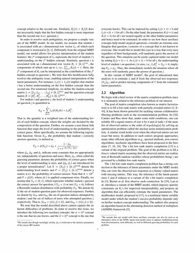
In order to resolve such ambiguities, we propose a simple vari-ant of the MIRT model. In our model, we assume that student iis associated with an r -dimensional row vector Li , of which eachcomponent is restricted to [0, 1]. Differently from the original MIRTmodel, our model allows for precise interpretation of the studentfeatures: the j th component of Li represents the level of student i’sunderstanding on the j th hidden concept. Similarly, question i isassociated with an r -dimensional row vector Ri 2 [0, 1]1⇥r , thecomponents of which sum up to 1, i.e.,

Prj=1 Ri (j ) = 1. Here, the

j th component of Ri can be interpreted as the contribution of the j th

hidden concept to question i. We note that this modification fullyresolves the ambiguity issue, enabling natural interpretation of thelatent parameters. For instance, Li (1) > Li (2) implies that studenti has a better understanding on the first hidden concept than thesecond one. For notational simplicity, we define the student-conceptmatrix L := [L1;L2; · · · ;Ln] 2 [0, 1]n⇥r and the question-conceptmatrix R := [RT1 ,R

T2 , . . . ,R

Tm] 2 [0, 1]m⇥r .

For student i and question j, the level of student i’s understandingon question j is quantified as

Xi j =rX

k=1Li (k )Rj (k ) = LiR

Tj .

That is, the quantity is a weighted sum of the understanding lev-els of each hidden concept, where the weights are dictated by thecomposition of the question. Further, we assume a non-linear linkfunction that maps the level of understanding to the probability ofcorrect guess. More specifically, we assume the following logisticlink function: Given Xi j , the probability that student i correctlyanswers question j is defined as

Pi j = � (Xi j ) = �a +1 � �a

1 + e��c (Xi j��b ) ,

where �a , �b , and �c indicate some constants that are appropriatelyset, independently of questions and users. Here, �a , often called theguessing parameter, denotes the probability of correct guess whenthe level of understanding is zero, and (�b ,�c ) are introduced fora proper normalization1. Let X := [Xi j ] 2 [0, 1]n⇥m denote theunderstanding level matrix and P := [Pi j ] 2 [0, 1]n⇥m denote amatrix w.r.t. the probability of correct-answer. Note that X = LRT

and P = � (X ), where � (·) is applied component-wise. Finally, weassume that Yi j 2 {0, 1}, which represents whether student i guessedthe correct answer for question j (Yi j = 1) or not (Yi j = 0), followsa Bernoulli random distribution with probability Pi j . We denote by� the set of student-question pairs for observed responses. Further,we denote by �i? and �?j the set of question indices attempted bystudent i and the set of indices of users who attempted question j,respectively. That is, �i? = {j |(i, j ) 2 �}, and �?j = {i |(i, j ) 2 �}.

We note that the model described above cannot capture the in-herent difficulties of problems. In order to resolve this issue, weintroduce the following two auxiliary concepts: the (r + 1)th conceptis the one that no one knows, and the (r + 2)th concept is the one that

1We remark that though seemingly similar, �b is irrelevant to the easiness parametersof the classic IRT models.

everyone knows. This can be imposed by setting Li (r + 1) = 0 andLi (r+2) = 1 for all i. On the other hand, the parameters Ri (r+1) andRi (r + 2) for all i are treated equally as the other hidden parameters,and hence need to be estimated. In order to see how these auxiliaryconcepts help model atypical questions, consider an extreme case.Imagine that question j consists of a concept that is not known toeveryone. One would like to model this case in a way that every user,regardless of their backgrounds, will randomly guess the answer ofthe question. This situation can be easily captured under our modelby setting Rj (r + 1) = 1. As Li (r + 1) = 0 for all i, the understandinglevel of student i on question j is zero, i.e., LiRTj = Xi j = 0, imply-ing Pi j = �a . Thus, this immediately models the situation where allthe users will randomly guess the answer of question j.

In this variant of MIRT model2, the goal of educational dataanalysis is to estimate L and R from the observed test responses(Yi j )� , and to predict missing components of Y from the estimatedlatent parameters.

2.2 AlgorithmWe begin with a brief review of the matrix completion problem sinceit is intimately related to the inference problem of our interest.

The goal of matrix completion (also known as matrix factoriza-tion) is to fill a low-rank matrix with partially revealed entires [2, 8–10]. It has been shown powerful for tackling various collaborativefiltering problems such as the recommendation problem. In [10],Candes and Rao show that, under some mild conditions, one canreliably fill a square matrix of size n by n and of rank r if the num-ber of observed entries is the order of nrpolylog(n) by solving anoptimization problem called the nuclear norm minimization prob-lem. A similar result holds even when the observed entries are notexact but noisy. In addition to such convex program approaches,many other efficient algorithms (e.g., spectral methods, non-convexalgorithms, stochastic algorithms) have been proposed in the liter-ature [7, 16, 24]. The 1-bit low-rank matrix completion [13] is avariant of the original problem. The goal of the problem is to fill abinary-valued matrix assuming that the observed entries are realiza-tion of Bernoulli random variables whose probabilities being 1 aregoverned by a hidden low-rank matrix.

The 1-bit low-rank matrix completion problem has a strong con-nection to the inference of latent parameters under the MIRT model.One can view the observed test responses as a binary-valued matrixwith missing entries. This way, the inference of the latent param-eters L and R reduces to a variant of the 1-bit matrix completion.In [3], Berner et al. first observe such connection. In [19], Lan etal. introduce a variant of the MIRT model, which imposes sparsityconstraints on Rj ’s for improved interpretability, and propose analgorithm that can efficiently estimate the latent parameters. Thedealbreaker model, proposed in [17], is a nonlinear latent variablemodel under which the student’s success probability depends onlyon his/her weakest concept understanding. The authors also proposean algorithm based on the alternating direction method of multipliers(ADMM) framework [5].

2We remark that our model with these auxiliary concepts can also be seen as analternative form of the M3PL latent trait model since it captures multidimensionalitem discrimination, item difficulty, as well as different guessing probability for eachproblem.

2

Algorithm 11: Input: observed responses (Yi j )(i, j )2� , index set �2: Initialize L(0) and R (0) uniformly at random in [0, 1].3: Normalize every R (0)

i such thatPrj=1 R

(0)i (j ) = 1.

4: k = 05: repeat6: L = L(k ) , R = R (k )

7: Shuffle �8: for (i, j ) in � do9: �L = 1 � µ�k

|�i? | , �R = 1 � µ�k|�?j |

10: � =�c⇣Yi j�� (LiRTj )

⌘

� (LiRTj ) (1+e��c (Li RTj ��b )

)

11: Li = �PL⇣�LLi + �Rj

⌘

12: Rj = �PR⇣�RRj + �Li

⌘

13: end for14: k = k + 115: L(k ) = L, R (k ) = R16: until convergence17: Output: L(k ) and R (k )

While the prior algorithms have shown superior prediction per-formances, most of them can hardly scale and/or can be hardly par-allelized. In order to design a scalable and parallelizable algorithmfor a large-scale educational data analysis, we develop an algorithmbased on the projected Stochastic Gradient Descent (SGD) method,which can be readily deployed on a parallel/distributed computingplatform as shown in [15, 24].

We now present our algorithm. Our algorithm is highly scalablesince its time and space complexities are linear in the number ofobserved test responses. Further, it is inherently online: an alreadytrained model can be efficiently retrained when new test responsesare revealed.

Our algorithm attempts to find the maximum likelihood (ML)estimator of X given a set of observation [Yi j ](i, j )2� . Equivalently,the ML estimator can be found by solving a minimization problemwhose objective function is the negative of the log likelihood ofthe observed entries. In order to encourage X to reflect a low-rankstructure, we also add to the objective function the nuclear norm reg-ularization term [10]. That is, we formulate an optimization problemas:

minL,R

X

(i, j )2�`(Yi j , Pi j ) + µkLRT k⇤

s.t. 0 Li j 1 , 0 Ri j 1 , 8i, j,P = � (LRT ),

X

jLi j = 1 , 8i ,

(P1)

where `(Yi j , Pi j ) indicates the negative log-likelihood of the ob-served response Yi j when P (Yi j = 1) = Pi j :

`(Yi j , Pi j ) = �Yi j log(Pi j ) � (1 � Yi j ) log(1 � Pi j ).We intend to approximate the optimization problem (P1) with (P2)(see below) by replacing the nuclear norm of LRT with the sumof the squared Frobenius norms of L and R. This approximation isbased on the following property [23]: the nuclear norm of a matrix

X is equal to the minimum sum of the squared Frobenius norms of Land R such that X = LRT .

minL,R

X

(i, j )2�`(Yi j , Pi j ) +

µ

2⇣kLk2F + kRk2F

⌘

s.t. 0 Li j 1 , 0 Ri j 1 , 8i, jP = � (LRT ),

X

jLi j = 1 , 8i .

(P2)

Indeed, any local minimum of (P2) is known to match that of theglobal minimum of the original problem (P1) under mild condi-tions, and this agreement can be further certified by checking rankdeficiency of L and R [24].

As a specific choice of the algorithm for solving (P2), we makeuse of the projected Stochastic Gradient Descent (SGD) method. Aformal description of our algorithm is given in Algorithm 1. Thealgorithm starts with randomly initialized L(0) and R (0) , and theniteratively updates sequences of L(k ) and R (k ) as follows. At thebeginning of each epoch, we randomly shuffle the index set �. Foreach pair of indices from �, say (i, j ), we update Li and Rj as inAlgorithm 1 where �PL (·) and �PR (·) are projections of a vectoronto the spaces of feasible L’s and R’s, respectively. This procedureis repeated until L(k ) and R (k ) converge. Note that each epoch’sruntime consists of time to shuffle data points and time to updateparameters |� | times. Since time to update parameter takes O (r ),the total time complexity, if a constant number of epochs is run, isO (r |� |).

Note that the projected SGD is known to converge to a globallyoptimal solution when the objective function and the regularizationterms (including those induced by constraints) are convex [21]. Theobjective function of (P2), however, is non-convex due to the prod-uct term LRT , so we run the above algorithm multiple times withdifferent initialization points.

A simple variation of our algorithm is the one intended for thecase when both R and the test response data set Y are given. It canbe shown that given R and observed responses Y� , the optimizationproblem (P2) reduces to a set of independent logistic regression prob-lems, each being with linear constraints. Hence, one can estimate Lby solving all of the logistic regression problems, and concatenatingthe estimated user features Li ’s.

2.3 Comparison with Existing AlgorithmsIn this section, we compare our proposed algorithms with the existingalgorithms in the literature. See Table 1 for the summary.

We first compare the algorithms that can estimate latent variables.As a specific instance of the IRT model, consider the two-parameterlogistic model (2PL) [20]. Assume that a gradient descent method isapplied to solve the corresponding ML estimation problem. The 2PLmodel assumes that the probability of correct guess depends on thesum of the user latent variable and the question latent variable. Whileit allows for less ambiguous interpretation of estimation results, itmay not be able to capture a complex structure due to its limitedmodel complexity. On the other hand, the original MIRT model [25]has the ability to express more complex models but fails to provideconsistent and interpretable estimation results. SPARFA [18], a vari-ant of the MIRT model, has much improved human interpretability

3

MODEL & ALGORITHM CLASSHUMAN-

INTERPRETABLEREQUIRES

RSCALABLE &

PARALLELIZABLEONLINE

2PL [20] IRT, AFFINE 3 7 7 7MIRT [25] MIRT, AFFINE 7 7 7 7SPARFA [19] MIRT, AFFINE 33 7 7 3DEALBREAKER [17] NONLINEAR 33 7 3 7OURS (SEC. 2.2) MIRT, AFFINE 3 7 3 3

G-DINA [14] NONLINEAR 33 3 7 7OURS WITH R (SEC. 2.2) MIRT, AFFINE 3 3 3 3

Table 1: Machine learning algorithms for educational data analysis

NAME n m |� | |� |/(nm)

FULL 123973 3835 8861570 1.86%FILTERED 16065 1999 2983327 9.29%

Table 2: Data sets

due to the sparse nature of their estimated parameters. More pre-cisely, by imposing sparsity constraints on R, their algorithm is ableto identify a few most important hidden concepts associated witheach question. Further, it scales well to high-dimensional problemssince it relies on a first-order method called the FISTA framework [1].However, it is not clear whether it can be easily parallelized. Onthe other hand, the dealbreaker model [17] is based on the ADMMframework [5], and hence can be easily parallelized.

Recall that when the precise estimate of R is provided, our al-gorithm reduces to multiple instances of convex problems, each ofwhich resembles logistic regression. This is because when R is fixed,the objective function and the constraints of (P2) can be decomposedinto n instances of a simple logistic regression. The G-DINA (gen-eralized deterministic inputs, noisy “and” gate) model [14] can bedeployed when such question tagging information is available, andallows for highly interpretable results. However, unlike our algo-rithm, the existing algorithms for the G-DINA model are neitherscalable nor parallelizable.

3 EXPERIMENTAL SETUP AND RESULTS3.1 Data SetWe first collected a pool of TOEIC (Test Of English for InternationalCommunication) questions. TOEIC is a test of English for interna-tional communication, and each test is composed of 150 multiple-choice questions with 4 options each. We first created the questionpool of 3835 TOEIC questions. With this question pool, we havecollected a large response data set via an online TOEIC educationplatform. From 1/1/2016 to 1/15/2017, a total of 123973 studentshad signed up for the platform, and a total of 8861570 responseshad been collected. Note the extremely low density of the responsematrix, which amounts to about 1.86%.

In order to obtain a high quality data set, we preprocess the rawdata set as follows. We first removed the students who had attemptedless than 30 questions during the observation period or had spentless than 3 seconds for more than or equal to 95% of their attempts.Similarly, we filtered out students whose correct answer rate is less

than or equal to 30%3 After we obtained the refined set of students,we filter out the questions that are responded less than 400 distinctstudents.

With the aforementioned filtering process, we obtained the filtereddata set consisting of |� | = 2983327 responses of n = 16065 studentson m = 1999 questions. Note that the density of the observationmatrix is about 9.29%. The size of the original data set and thefiltered data set are summarized in Table 2.

3.2 Algorithm Implementation and SpecificationWe randomly divide the filtered data set into the training set (90%)and the test set (10%). All the experiment results reported in thissection are with respect to the test set. We then conduct a heuristicoptimization for finding the optimal hyper-parameters such as theregularization parameter µ, the sequence of step sizes, and etc. As aresult, we chose µ = 1; the step size is initialized as �0 = 0.1, and isdecreased by a multiplicative factor of 100.3 whenever the validationscore stops improving for 3 epochs in a row. For the link function� (·), we use �a = 0.25, �b = 0.5 and �c = 10. The rationale behindthese choices is that one can correctly guess the answer of a questionwithout knowing anything about a 4-choice question with probabilityat least 0.25.

We implement our algorithm in Python. In addition to our ap-proach, we also evaluate the prediction performances of some ofthe approaches described in Sec. 2.3: we fit our data set to the 2PLmodel [20] using mirt R package [11], and to the vanilla MIRTmodel [25] using the 1-bit matrix completion algorithm of [13].

3.3 Prediction PerformanceIn this section, we evaluate the prediction performances of variousalgorithms. More precisely, we run various algorithms with thetraining set and measure the prediction (classification) performances.A prediction outcome for an unobserved test response is called a truepositive (negative) if the predictor correctly guessed that the studentwill respond to the question with a correct (wrong) answer. Similarly,a prediction outcome is a false positive (negative) if the predictormade a wrong guess that the student will respond to the question witha correct (wrong) answer. We denote the number of true positives,false positives, true negatives, and false negatives by tp, fp, tn, andfn, respectively. For the performance metric, we consider the area

3The rationale behind these filtering conditions is that students not satisfying theseconditions are likely to be ones who simply wanted to try out and explore the mobileapplications for fun.

4

ALGORITHM AUC NLL

M2PL 0.7775 0.5209MIRT (L,r = 2) 0.7674 0.5413MIRT (L,r = 4) 0.7695 0.5361MIRT (P,r = 2) 0.7696 0.5338MIRT (P,r = 4) 0.7692 0.5320OURS (r = 2) 0.7760 0.5223OURS (r = 4) 0.7707 0.5277

Table 3: Prediction performances on the filtered data set. AUCdenotes the area under curve (AUC) of a receiver operatingcharacteristic (ROC) curve, and NLL denotes the negative oflog likelihood. For the MIRT model, we test both logistic linkfunctions (denoted by ‘L’) and probit link function (denoted by’P’). For the MIRT model and our algorithm, we vary the num-ber of hidden concepts r 2 {2, 4}.

under curve (AUC) of a receiver operating characteristic (ROC)curve. For a classification threshold � 2 [0, 1], the ROC curve isa collection of pairs (fpr(� ), tpr(� )). Note that the ROC curve of arandom predictor is a line segment connecting (0, 0) and (1, 1), andthat of a perfect predictor is line segments connecting (0, 0), (0, 1),and (1, 1). Thus, the area under curve (AUC) of a ROC curve canrepresent the classification performance of a predictor: the larger theAUC is, the better the prediction performance is. We also measurethe negative of log likelihood (NLL) of each prediction algorithm.

The prediction performances of various learning algorithms aresummarized in Table 3. For the MIRT model, we test both logisticlink function (denoted by ‘L’) and probit link function (denotedby ’P’). For the MIRT model and our algorithm, we evaluate theprediction performances with r 2 {2, 4}. We observe that whenwe set r > 4, the prediction performance is strictly worse4. Foreach configuration, the AUC and NLL are measured 20 times withrandomly divided data sets, and the average values are shown. Wecan see that the best prediction performance is achieved by the M2PLmodel, and our algorithm closely matches the best performance.

Thanks to the scalability of our algorithm, we could also measurethe AUC performance of our algorithm w.r.t. the full data set: theaverage AUC is observed to be 0.7778.

3.4 Tag Correction via Interpretable ResultsIn a large-scale education system, questions are associated with‘concept tags’, and such associations are usually judged by expertsin a manual way. However, such tagging information is prone toerrors due to human errors, inherent ambiguity, atypical questions,etc. Thus, identifying those wrongly tagged questions and correctingthem are a key to maintain high-quality tagging information, whichis crucial for providing suitable learning materials in a personalizededucation system.

We first explain how the improved interpretability of our modelallows for an efficient tag correction procedure. First, if there existthe sign ambiguity and the scale ambiguity, the question features ofsimilar questions are not necessarily close to each other. Secondly,

4Note that choosing a larger value for r , the upper bound on the true rank, does notnecessarily improve the prediction performance due to overfitting.

question features obtained under ambiguous models are not invariantacross different training instances. For example, when one has torerun the training algorithm from scratch for some reasons (suchas new dataset arrival, batch model update, algorithm modification,etc.), all question features change, and such a tagging correctionprocedure has to be restarted from scratch.

Leveraging the improved interpretability of our algorithm, we nowpresent a systematic way of identifying wrongly tagged questions.Consider the case of r = 2. Under our model, the quantity � =Ri (1)/(Ri (1) + Ri (2)) can be interpreted as the relative fraction ofhidden concept 1 w.r.t. question i. If our model can well explain thedata set, questions of the same type are supposed to have similarvalues of � . Thus, by inspecting the values of � of the questionsannotated with the same tag, one may be able to detect wronglytagged questions.

In order to conduct the experiment, we had a small subset of theTOEIC question pool tagged by experts as follows. The 15 hiredexperts first investigated the question pool, and then came up witha set of 69 tags, which were considered useful and necessary fordescribing the questions in the question pool. More specifically,each question was randomly assigned to at least two experts, andthe experts tagged each of the assigned questions with the mostrelevant concept. We develop an online tagging system where theexperts were able to individually work on the assigned questions.In order to reduce systematic bias between experts, we revealed thefirst reviewer’s response to a question to the second reviewer of thequestion so that the second reviewer can adjust the response of thefirst reviewer5.

After every question is tagged, we compare the values of � of thequestions of the same tag, and identified a large number of wronglytagged questions, of which a few instances are shown below. Weplot in Fig. 1 the values of � of all the questions tagged with the tag‘for oneself/by oneself/on one’s own’. There are 12questions, denoted by Qi for i 2 [12], which are identified as ques-tions that require the understanding on the usage of ‘for oneself’, ‘byoneself’, or ‘on one’s own’. These questions are for testing whetherstudents can fill a blank in a sentence with a grammatically correctword or phrase. Each question is tagged with the key phrase that oneneeds to fully understand in order to correctly answer the question.However, we can observe 3 clusters of the questions: the first clusterconsisting of Q1 and Q2, the second one in the middle, and the thirdone consisting of Q9 to Q12.

It turns out that the questions in the first and third clusters areassociated with incorrect tags. Table. 4 shows two correctly taggedquestions and two incorrectly tagged ones. It is clear that the firsttwo questions are about ‘for oneself’ but the other two questions areirrelevant to the tag. For instance, Q10 is asking whether studentscan fill the missing pronoun ‘them’. We conjecture that this problemis wrongly tagged because the problem may seem relevant to theconcept on one’s own. Similarly, Q11 is clearly wrongly taggedsince it is about whether students can fill the missing blank with acorrect reflexive pronoun.

5We could not measure inter-rater reliability (IRR) since the responses of differentexperts were dependent under our scheme.

5

(Q1)ontheirown

(Q2)onyourown (Q4)byhimself

(Q3)bythemselves

(Q5)byhimself

(Q6)ofhisown

(Q7)forherself

(Q8)forthemselves

(Q9)devotedhimself

(Q10)logoonthem

(Q11)thinkofyourself

(Q12)viewofitsown

� = 0 � = 1

Figure 1: � values of the questions tagged with ‘for oneself/by oneself/on one’s own’

Q7. MS. GRANT HAS ASKEDFOR A MINI-BUS FROM THEAIRPORT TO THE CLIENT’S OF-FICES FOR (HERSELF) ANDTHE ENTIRE SALES TEAMTHIS MONDAY.

Q8. THE MANUFACTURINGPLANT’S POLICY ALLOWS WORK-ERS TO SPEAK FOR (THEMSELVES)IN CASES WHERE COMPENSATION ISSOUGHT FOR AN INJURY SUFFEREDON THE JOB.

Q10. THE COMPANY PULLEDTHEIR T-SHIRTS OFF FROMSTORE SHELVES WHEN THE PUB-LIC COMPLAINED ABOUT THEOFFENSIVE LOGO ON (THEM).

Q11. IT’S NEVER A GOODIDEA TO THINK OF (YOUR-SELF) AS SUPERIOR TOYOUR SUPERIORS, OR YOUJUST MIGHT GET FIRED.

Table 4: A few questions tagged with ‘for oneself/by oneself/on one’s own’

(a) Prediction accuracy as a function ofthe number of questions solved by a user

(b) Prediction accuracy as a function ofthe number of responses for a question

Figure 2: Prediction performance as a function of the numberof per-student, per-question observations.

4 CONCLUSIONIn this work, we proposed a new algorithm based on a human-interpretable MIRT model, which is both scalable and parallelizable.Using the large data set collected from an online education platform,we observe that our algorithm can achieve as good prediction perfor-mance as the state of the arts. Moreover, we show that the improvedinterpretability of our model allows for an efficient and systematicway of identifying wrongly tagged questions. We conclude the paperby discussing a few interesting open problems and some aspects ofour current model that are subject to improvements.

4.1 Correlation Between the Number ofResponses and Prediction Accuracy

In our data set, the number of responses per student and the numberof responses per question widely vary. One important question is:how the prediction performance changes when the number of ques-tions per student (or per question) increases. To answer this question,we first bin the students according to the number of responses perstudent, and then micro-average the prediction accuracies of thestudents of the same bin. Similarly, we bin the questions according

to the number of responses per question, and then micro-average theprediction accuracies. Plotted in Fig. 2 are micro-averaged accuracyas a function of the number of questions attempted by students andthat as a function of the number of responses per question. We usethe bin size of 50 for Fig. 2(a), and the bin size of 250 for Fig. 2(b).From Fig. 2(a), we can observe that the predicted accuracy of astudent’s responses linearly increases as the number of questionssubmitted by the student increases. Similarly, the predicted accuracyof the responses for a question linearly increases with the number ofresponses for the question. Thus, one can determine using this proce-dure the number of responses per student or per question with whicha personalized education system can provide prediction serviceswith high enough accuracy.

4.2 Incorporation of Other Forms of DataWhile we used the binary response data only, the actual responsedata set contains several additional sources of side information suchas the option chosen by students, the options marked wrong bystudents, the time taken to respond to a question, and etc. By incor-porating the other forms of data with a more complicated model,one may be able to obtain better estimates of students and questions,and hence to provide superior prediction performance as well aspersonalized learning of a better quality. For instance, the nominalresponse model (NRM) proposed in [4] can model the probabilityof students responding to a certain option of a question. In [22],Ning et al. propose a new model for option responses with human-interpretable outputs, and show that the new model fits better withreal world data as well. It is an interesting future direction to studyhow one can apply a similar collaborative filtering-approach undersuch models capturing option responses. In [6], Brinton et al. showthat one can predict students’ future performances on quizzes usingvideo-watching clickstream data from MOOCs. It is an interestingopen question whether a unified model that uses both response dataand video-watching clickstream data can achieve higher predictionperformance.

6

4.3 Time-varying LOur response model implicitly assumes that the level of students’understanding is time-invariant. If the data set is collected over along time period during which student’s level of understanding islikely to fluctuate, such an assumption may totally fail, and theestimated L will be close to the time average of L, which is lessinformative for predicting future responses.

If one is given with an enormous amount of data, there is a simplefix: one can simply keep fresh responses collected over a short timeperiod only: a time-invariant model for students’ understanding willfit better for a shorter range of time. The number of responses in thedataset, however, decreases when one reduces the data collectionperiod, possibly deteriorating the prediction performance.

In order to resolve this issue, in [18], Lan et al. have proposed atime-variant model for learning analytics capturing the time varyinglevels of understanding of learners. We believe that such a time-variant model can take advantage of a large amount of data withoutcompromising the fitness of the model.

4.4 Sparsity of RWhile it is reasonable to believe that among many concepts only afew are required to correctly answer a question, we observe that ourcollaborative filtering algorithm usually results in a dense question-concept matrix R. Therefore, imposing sparsity on R can potentiallyallow for a better model and hence an improved prediction per-formance. In [19], Lan et al. propose a collaborative filtering thatcan find a sparse question-concept matrix R by incorporating the `1regularization term into the objective function of the optimizationproblem. The authors observe a superior prediction performance oftheir proposed sparse model compared with the non-sparse modelproposed in [3]. Inspired by this observation, we also measured theperformance of the variation of our algorithm where the `1 regular-ization term is incorporated but we did not observe an improvementin prediction performance with our data set. Even though we couldnot observe an improvement in prediction performance with our dataset, we believe that the sparse models, capturing the natural sparsityof R, will result in more accurate estimates in general.

4.5 Mixture Models and Outlier DetectionAll the models described in this paper assume a common assump-tion: one model fits all the students and questions. This could be thecase for small-scale educational data such as those collected fromclassrooms but not for data collected from a large-scale educationplatform with hundreds of thousands of students with completelydifferent backgrounds. For instance, in an online education systemwhere students freely choose questions to work on and do not getpenalized for guessing wrong answers, some students might reck-lessly solve questions, resulting in random responses, which do notconform existing response models. Similarly, some questions in alarge question pool may not conform the typical pattern of the otherquestions. Hence, an accurate mixture model capturing such outlierscan greatly enhance the performance prediction.

REFERENCES[1] Amir Beck and Marc Teboulle. 2009. A fast iterative shrinkage-thresholding

algorithm for linear inverse problems. SIAM journal on imaging sciences 2, 1(2009), 183–202.

[2] Robert Bell, Yehuda Koren, and Chris Volinsky. 2007. Modeling relationships atmultiple scales to improve accuracy of large recommender systems. In Proceed-ings of the 13th ACM SIGKDD international conference on Knowledge discoveryand data mining. ACM, 95–104.

[3] Yoav Bergner, Stefan Droschler, Gerd Kortemeyer, Saif Rayyan, Daniel Seaton,and David E Pritchard. 2012. Model-Based Collaborative Filtering Analysis ofStudent Response Data: Machine-Learning Item Response Theory. InternationalEducational Data Mining Society (2012).

[4] R Darrell Bock. 1972. Estimating item parameters and latent ability when re-sponses are scored in two or more nominal categories. Psychometrika 37, 1(1972), 29–51.

[5] Stephen Boyd, Neal Parikh, Eric Chu, Borja Peleato, and Jonathan Eckstein.2011. Distributed optimization and statistical learning via the alternating directionmethod of multipliers. Foundations and Trends® in Machine Learning 3, 1 (2011),1–122.

[6] Christopher G Brinton, Swapna Buccapatnam, Mung Chiang, and H Vincent Poor.2016. Mining MOOC Clickstreams: Video-Watching Behavior vs. In-Video QuizPerformance. IEEE Transactions on Signal Processing 64, 14 (2016), 3677–3692.

[7] Jian-Feng Cai, Emmanuel J Candès, and Zuowei Shen. 2010. A singular valuethresholding algorithm for matrix completion. SIAM Journal on Optimization 20,4 (2010), 1956–1982.

[8] Emmanuel J Candes and Yaniv Plan. 2010. Matrix completion with noise. Proc.IEEE 98, 6 (2010), 925–936.

[9] Emmanuel J Candès and Benjamin Recht. 2009. Exact matrix completion viaconvex optimization. Foundations of Computational mathematics 9, 6 (2009),717–772.

[10] Emmanuel J Candès and Terence Tao. 2010. The power of convex relaxation:Near-optimal matrix completion. IEEE Transactions on Information Theory 56, 5(2010), 2053–2080.

[11] R Philip Chalmers and others. 2012. mirt: A multidimensional item responsetheory package for the R environment. (2012).

[12] John Daniel. 2012. Making sense of MOOCs: Musings in a maze of myth, paradoxand possibility. Journal of interactive Media in education 2012, 3 (2012).

[13] Mark A Davenport, Yaniv Plan, Ewout van den Berg, and Mary Wootters. 2014.1-bit matrix completion. Information and Inference 3, 3 (2014), 189–223.

[14] Jimmy De La Torre. 2011. The Generalized DINA Model Framework. Psychome-trika 76, 2 (2011), 179–199. https://doi.org/10.1007/s11336-011-9207-7

[15] Rainer Gemulla, Erik Nijkamp, Peter J Haas, and Yannis Sismanis. 2011. Large-scale matrix factorization with distributed stochastic gradient descent. In Proceed-ings of the 17th ACM SIGKDD international conference on Knowledge discoveryand data mining. ACM, 69–77.

[16] Prateek Jain, Praneeth Netrapalli, and Sujay Sanghavi. 2013. Low-rank matrixcompletion using alternating minimization. In Proceedings of the forty-fifth annualACM symposium on Theory of computing. ACM, 665–674.

[17] Andrew Lan, Tom Goldstein, Richard Baraniuk, and Christoph Studer. 2016.Dealbreaker: A Nonlinear Latent Variable Model for Educational Data. In Pro-ceedings of the 33rd International Conference on International Conferenceon Machine Learning - Volume 48 (ICML’16). JMLR.org, 266–275. http://dl.acm.org/citation.cfm?id=3045390.3045420

[18] Andrew S Lan, Christoph Studer, and Richard G Baraniuk. 2014. Time-varyinglearning and content analytics via sparse factor analysis. In Proceedings of the20th ACM SIGKDD international conference on Knowledge discovery and datamining. ACM, 452–461.

[19] Andrew S Lan, Andrew E Waters, Christoph Studer, and Richard G Baraniuk.2014. Sparse factor analysis for learning and content analytics. Journal ofMachine Learning Research 15, 1 (2014), 1959–2008.

[20] Frederic M Lord. 1980. Applications of item response theory to practical testingproblems. Routledge.

[21] Arkadi Nemirovski, Anatoli Juditsky, Guanghui Lan, and Alexander Shapiro.2009. Robust stochastic approximation approach to stochastic programming.SIAM Journal on optimization 19, 4 (2009), 1574–1609.

[22] Ryan Ning, Andrew E Waters, Christoph Studer, and Richard G Baraniuk. 2015.SPRITE: A Response Model For Multiple Choice Testing. arXiv preprintarXiv:1501.02844 (2015).

[23] Benjamin Recht, Maryam Fazel, and Pablo A Parrilo. 2010. Guaranteed minimum-rank solutions of linear matrix equations via nuclear norm minimization. SIAMreview 52, 3 (2010), 471–501.

[24] Benjamin Recht and Christopher Ré. 2013. Parallel stochastic gradient algorithmsfor large-scale matrix completion. Mathematical Programming Computation 5, 2(2013), 201–226.

[25] Mark Reckase. 2009. Multidimensional item response theory. Vol. 150. Springer.[26] George Siemens. 2010. What are learning analytics? http://www.elearnspace.org/

blog/2010/08/25/what-are-learning-analytics/. (2010). Accessed: 2016-09-30.

7