lascad tutorial no. 2: modeling a laser cavity with side ... · lascad tutorial no. 2: ... the...

LASCAD Tutorial No. 2: Modeling a laser cavity with side pumped rod

Revised January 19, 2009

© Copyright 2006-2009 LAS-CAD GmbH

Table of Contents 1

Table of Contents 1 Starting LASCAD and Defining a Simple Laser Cavity............................................................. 3 2 Defining and Analyzing a Side Pumped Rod.............................................................................. 4

2.1 Selecting crystal type and pump configuration.................................................................... 4 2.2 Defining the pump light distribution.................................................................................... 5 2.3 Defining cooling of the rod .................................................................................................. 8 2.4 Defining material parameters............................................................................................. 10 2.5 Defining composite material .............................................................................................. 11 2.6 Defining options to control the FEA computational procedure ......................................... 11 2.7 Visualizing results of the FEA ........................................................................................... 13

2.7.1 3D Visualizer ............................................................................................................. 13 2.7.2 2D Data Profiles and Parabolic Fit ............................................................................. 14

2.8 Computing gaussian modes................................................................................................ 15 2.9 Inserting the crystal into the mode plot.............................................................................. 16

3 Modifying cavity parameters..................................................................................................... 17 4 Tools to analyze the properties of a laser cavity ....................................................................... 17

4.1 Analyzing stability of a laser cavity................................................................................... 17 4.2 Showing transverse gaussian mode profile ........................................................................ 18 4.3 Computing the laser power output ..................................................................................... 19

5 The Beam Propagation Code (BPM)......................................................................................... 21

Note: The project file Tutorial_2.lcd of the example used with this tutorial can be found in the directory Tutorials on the CD-ROM or after installation of LASCAD in the subdirectory Tutorials of the LASCAD application directory. You can copy this file to a working direc-tory.

Note: The numerical results shown in this tutorial are obtained, if for the computation the demo ver-sion of the LASCAD program is used. The wavelength in the demo version is fixed to 1134 nm which differs somewhat from the wavelength of a Nd:YAG laser. To obtain the correct results open Tutorial_2.lcd with the full version.

Selecting crystal type and pump configuration 3

1 Starting LASCAD and Defining a Simple Laser Cavity • Start LASCAD, • Define a working directory, • Click OK to open the LASCAD main window, • Click the New Project button on the toolbar (leftmost button), or use the menu item

File→New, • Increase the Number of Face Elements to 4, • Enter the appropriate wavelength (not possible with demo version), and leave the other de-

fault settings unchanged, • Click OK.

Now you can see the LASCAD main menu at the top and two other windows below. The upper one is titled Standing Wave Resonator, the lower one Parameter Field, as shown Fig. 1. The

Fig. 1

4 Defining and Analyzing a Side Pumped Rod

upper window shows the mode plot of a simple cavity with four elements; the lower window shows the parameters of the cavity. In the column below the element number, the parameters belonging to this element are shown, such as the radius of curvature of each mirror, in the row labeled Type-Param.. To change the element type use the drop-down boxes immediately below the element number. You can select from Mirror, Dielectric Interface, and Lens. The parame-ters of the columns between the element numbers define the properties of the space between the elements, such as the refractive index, or the Refractive Parameter, which corresponds to the second derivative of a parabolic refractive index distribution. Information about additional func-tionalities of these windows for instance "How to insert or clear an element?" can be found in in the online help, in the the Quick Tour, or in the manual.

2 Defining and Analyzing a Side Pumped Rod 2.1 Selecting crystal type and pump configuration Select FEA→Parameter Input & Start of FEA Code, in the main LASCAD window, to open the window titled Crystal, Pump Beam and Material Parameters, as shown in Fig. 2. Note the six tabs which allow for defining various groups of parameters.

Fig. 2

Defining the pump light distribution 5

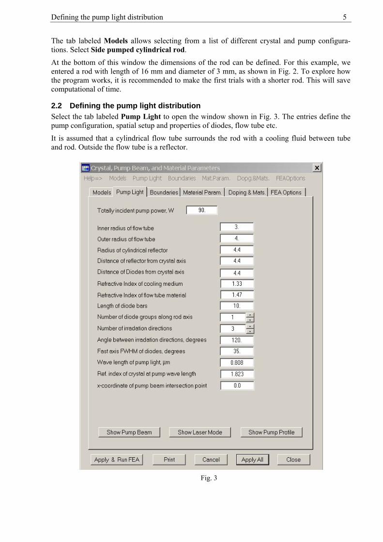
The tab labeled Models allows selecting from a list of different crystal and pump configura-tions. Select Side pumped cylindrical rod.

At the bottom of this window the dimensions of the rod can be defined. For this example, we entered a rod with length of 16 mm and diameter of 3 mm, as shown in Fig. 2. To explore how the program works, it is recommended to make the first trials with a shorter rod. This will save computational of time.

2.2 Defining the pump light distribution Select the tab labeled Pump Light to open the window shown in Fig. 3. The entries define the pump configuration, spatial setup and properties of diodes, flow tube etc.

It is assumed that a cylindrical flow tube surrounds the rod with a cooling fluid between tube and rod. Outside the flow tube is a reflector.

Fig. 3


Totally incident pump power is the pump power incident from all diodes together on the rod.

Inner radius of flow tube and Outer radius of flow tube are the inner and outer radius of the flow tube, respectively. If no flow tube is present in your model, define the outer radius very close to the inner the radius, and set the refractive index of the flow tube material equal to the refractive index of the fluid.

Radius of cylindrical reflector is the radius of a cylindrical reflector used to reflect the pump beam back into the rod after having passed the rod a first time.

The Distance of reflector from rod axis must not necessarily be identical with the radius of the reflector though it is in most cases. However, the reflector also can be plane, for instance. If no reflector is present enter a large value for this parameter.

If you have several groups of diodes surrounding the rod, the meaning of Length of diode bars and Number of diode groups along rod axis depends on the arrangement of the diodes.

If the diodes are set up along a light emitting line parallel to the rod axis, enter the length of this line for Length of diode bars and "1" for Number of diode groups along rod axis.

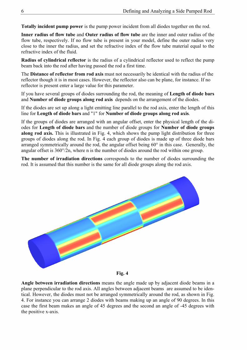
If the groups of diodes are arranged with an angular offset, enter the physical length of the di-odes for Length of diode bars and the number of diode groups for Number of diode groups along rod axis. This is illustrated in Fig. 4, which shows the pump light distribution for three groups of diodes along the rod. In Fig. 4 each group of diodes is made up of three diode bars arranged symmetrically around the rod, the angular offset being 60° in this case. Generally, the angular offset is 360°/2n, where n is the number of diodes around the rod within one group.

The number of irradiation directions corresponds to the number of diodes surrounding the rod. It is assumed that this number is the same for all diode groups along the rod axis.

Angle between irradiation directions means the angle made up by adjacent diode beams in a plane perpendicular to the rod axis. All angles between adjacent beams are assumed to be iden-tical. However, the diodes must not be arranged symmetrically around the rod, as shown in Fig. 4. For instance you can arrange 2 diodes with beams making up an angle of 90 degrees. In this case the first beam makes an angle of 45 degrees and the second an angle of -45 degrees with the positive x-axis.

Fig. 4

Defining the pump light distribution 7

Fast axis FWHM of diodes, degrees (Full Width Half Max) usually is specified in the diode data sheet.

Wavelength of pump light and Refractive index of crystal at pump wavelength are self-explaining and are used to compute the propagation of the pump beam through the rod.

x-coordinate of pump beam intersection point can be used to define a small (not more than a few percent of the rod diameter) displacement of this point with respect to the rod axis. This may be desirable in case of unsymmetrical irradiation.

In the slow axis direction a top hat profile is assumed for the pump beam. The rays of the pump beam are assumed to propagate perpendicular to the rod axis. The slow axis divergence can ap-proximately be taken into account by increasing the entry for the length of the diode bars.

In fast axis direction the shape of the propagating pump beam is computed by the use of the gaussian ABCD algorithm. The fast axis divergence angle of the pump beam is computed as

015.0*))5.0ln((2*360* FWHMFWHM ≈−°° π [rad]. The fast axis profile is assumed to be gaussian, which means that the intensity distribution in fast axis direction axis is assumed to be proportional to exp[-2(s/σ)²], where σ depends on the distance from the emitting surface of the diode.

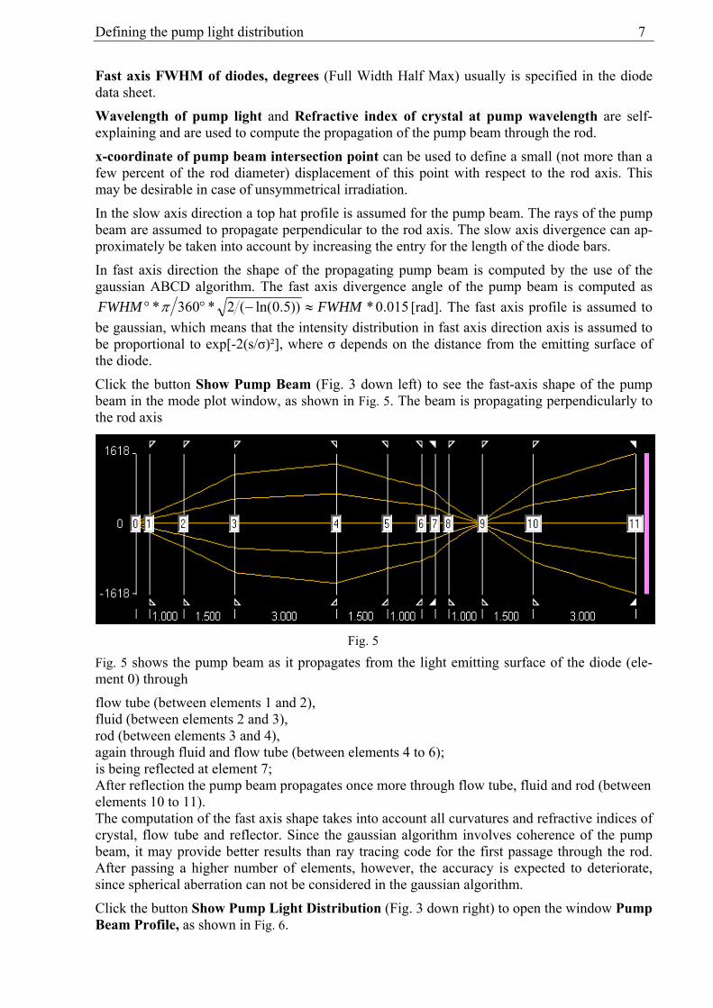
Click the button Show Pump Beam (Fig. 3 down left) to see the fast-axis shape of the pump beam in the mode plot window, as shown in Fig. 5. The beam is propagating perpendicularly to the rod axis

Fig. 5 shows the pump beam as it propagates from the light emitting surface of the diode (ele-ment 0) through

flow tube (between elements 1 and 2), fluid (between elements 2 and 3), rod (between elements 3 and 4), again through fluid and flow tube (between elements 4 to 6); is being reflected at element 7; After reflection the pump beam propagates once more through flow tube, fluid and rod (between elements 10 to 11). The computation of the fast axis shape takes into account all curvatures and refractive indices of crystal, flow tube and reflector. Since the gaussian algorithm involves coherence of the pump beam, it may provide better results than ray tracing code for the first passage through the rod. After passing a higher number of elements, however, the accuracy is expected to deteriorate, since spherical aberration can not be considered in the gaussian algorithm.

Click the button Show Pump Light Distribution (Fig. 3 down right) to open the window Pump Beam Profile, as shown in Fig. 6.

Fig. 5


Moving the slider arranged below the plot does not change the pump profile, since it is assumed to be constant along the rod axis. However the absorbed power density disappears, if you are moving the slider to the ends of the rod outside the pumped region.

2.3 Defining cooling of the rod Select the tab labeled Boundaries to open the window shown in Fig. 7 The entries allow defining cooling conditions individually for each surface of the rod.

You can define cooling as either by solid or fluid contact. For the fluid contact, additionally check the box Fluid Cooling.

In case of solid cooling, the surface is kept at constant temperature, which is defined by the value in the box Temperature, K. For fluid cooling, the latter value defines the bulk tempera-ture of the fluid.

Fig. 6

Defining cooling of the rod 9

In case of fluid cooling a film coefficient, which describes the heat transfer through the interface solid-fluid, must also be defined (bottom row in Fig. 7). Section 6.10.3 of the LASCAD manual describes this in more detail.

The entry for Reference temperature is used with computation of deformation and corresponds to the crystal temperature before heating. When boundary temperatures are defined in the Kelvin scale, it is important to enter here the correct value.

Cooling must not extend along the full length of the barrel surface, which usually is not the case for side pumping. The entries into the row Surface extends from z= … to … allow defining the exact point where the cooled surface begins and where it ends. In the case shown in Fig. 7, the cooled surface begins at z = 2 and ends at z = 14 mm. Both ends of the 16 mm long rod are not cooled. The origin of the coordinate system is located in the center of the left end face of the rod.

Cooling of the end faces of the rod does not usually apply in side pumping.

If you use temperature dependent material parameters or 3-level-materials, it is important to use the Kelvin scale here. Otherwise you can enter the value "0" for the cooled surfaces.

Fig. 7


2.4 Defining material parameters Select the tab Material Param. to open the window shown in Fig. 8.

The entries are almost self-explaining. The absorption coefficient describes the exponential at-tenuation of the pump beam, according to )exp()( 0 zIzI α−= . Due to absorption of the pump photons, it depends on the doping level of the crystal. Details are described in the appendix of the manual.

In the lower part of the window more sophisticated issues can be defined, like temperature de-pendent material parameters, or solids composed of two different materials, as described in the manual sect. 6.10.4.

You can save the material parameters to a file and use them later with a new project.

Fig. 8

Defining composite material 11

2.5 Defining composite material Select the tab Doping & Mats. to open the window shown in Fig. 9.

In the case of side pumping, laser materials composed of doped and un-doped sections usually are not applied. Therefore the entries shown in Fig. 9 are zero or large numbers.

An example with an end pumped rod with undoped end-caps is described in Tutorial 1.

The appearance of this window depends on options selected in the tab Material Param.

2.6 Defining options to control the FEA computational procedure

Select the tab FEA Options to open the window shown in Fig. 10.

The Finite Element Analysis (FEA) code uses a regular rectangular mesh inside the crystal, which is connected to the boundaries of the crystal by small irregular elements.

Mesh size in x- and y-direction is the edge length of the voxels perpendicular to the crystal axis.

Mesh size in z-direction is the edge length of the voxels along the crystal axis.

Click Estimated number of elements to get information concerning the amount of memory needed to run the computation. The following rule of thumb can be used: If you have n ele-ments, you should have roughly 2*n/1000 MB RAM available, otherwise the program becomes very slow, as memory is paged to disk. (You can use the Windows Task-manager to determine the amount of free RAM currently available, which can usually be opened by pressing Ctrl-Alt-Del. Open the tab System Performance. The row Available in the box Physical Memory dis-plays an estimate of currently available memory.)

The entries for Convergence limits control the convergence of the iterative computational pro-cedure. The default value 1.0E-7 for the thermal analysis stops the code if the temperature maximum does not change within the first 7 digits. The limit for the structural analysis refers to the absolute value of maximum nodal displacement.

Regardless of the convergence limits, the iteration process is stopped, if the number of iterations exceeds the numbers entered in Maximum number of iterations.

The input box, Directory for output of FEA results, can be used to define a directory where the files created by the FEA code are stored. Default setting is the subdirectory FEA of the Working Directory.

Fig. 9


The input box, Position of cutting plane perpendicular to z-axis, allows for placing a cutting plane perpendicular to the z-axis, to show the distribution of physical quantities inside the crys-tal with the 3D Visualizer, as described in the next section. If the value 0 is entered, a cutting plane along the rod axis and perpendicular to the y-axis is used. If the entry is greater than zero and smaller than the rod length, a cutting plane perpendicular to the rod axis is used. If the entry is greater than the rod length, the full crystal is shown.

Use the button Apply and run FEA to transfer the input data to internal variables and to start the FEA code. The window Finite Element Analysis pops up showing the number of the cur-rently running iteration. In addition, it shows the maximum temperature during thermal analysis, and the absolute value of maximum nodal displacement during structural analysis. At the end of the computation, the message "FEA finished successfully" appears. Click OK to close the dia-log.

Fig. 10

Visualizing results of the FEA 13

Please be aware that initialization of the FEA and generation of the mesh may take some time for large element numbers.

2.7 Visualizing results of the FEA LASCAD provides 3D and 2D tools to visualize the FEA results data.

2.7.1 3D Visualizer To show 3D plots of the FEA results, select FEA→3D Visualizer in the main LASCAD menu. It opens an easy-to-handle 3D Visualizer based on OpenGL. As examples, 3D plots of heat load and temperature distribution are shown in Fig. 11 and Fig. 12, respectively. The plots show the distributions from z = 0 up to a cutting plane perpendicular to the rod at z = 8 mm, the latter value has been defined as input into box Position of cutting plane … in the tab FEA Options.

Fig. 11

Fig. 12


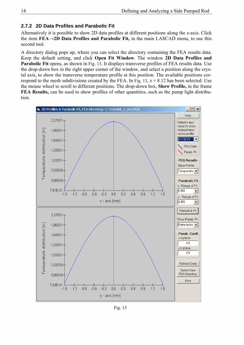
2.7.2 2D Data Profiles and Parabolic Fit Alternatively it is possible to show 2D data profiles at different positions along the z-axis. Click the item FEA→2D Data Profiles and Parabolic Fit, in the main LASCAD menu, to use this second tool.

A directory dialog pops up, where you can select the directory containing the FEA results data. Keep the default setting, and click Open Fit Window. The window 2D Data Profiles and Parabolic Fit opens, as shown in Fig. 13. It displays transverse profiles of FEA results data. Use the drop-down box in the right upper corner of the window, and select a position along the crys-tal axis, to show the transverse temperature profile at this position. The available positions cor-respond to the mesh subdivisions created by the FEA. In Fig. 13, z = 8.12 has been selected. Use the mouse wheel to scroll to different positions. The drop-down box, Show Profile, in the frame FEA Results, can be used to show profiles of other quantities, such as the pump light distribu-tion.

Fig. 13

Computing gaussian modes 15

2.8 Computing gaussian modes To use the FEA results with the gaussian mode-algorithm, the profiles of the temperature in-duced refractive index and the thermal deformation of the crystal end faces of the rod must be fitted parabolically, transverse to the optical axis.

In advance, a Range of Fit has to be defined, which, depending on the expected spot size of the mode, can usually can be much smaller than the diameter of the crystal. We select 0.4 mm for the range of fit.

Click Refresh & Fit, in the frame Parabolic fit, to carry through the parabolic fit, as shown in Fig. 14. The red lines represent the parabolic curves, and the blue lines the FEA results, respec-tively. The good overlap of both lines is showing that the temperature distribution computed by FEA is very close to a parabolic curve in the present case.

Fig. 14


The fit is computed for all subsections along the crystal axis generated by the FEA meshing pro-cedure. That means that the crystal is subdivided into a series of GRIN lenses each of them hav-ing its individual parabolic refractive index distribution. The left end face of the leftmost sub-section coincides with the left end face of the crystal; correspondingly the right face of the right-most subsection coincides with the right end face of the crystal. The deformation of these end faces is taken into account by fitting the radii of curvature of astigmatic spherical surfaces to these end faces.

Again, you can use the drop-down box in the right upper corner of the window to show the fit at different positions along the z-axis. The parabolic coefficients obtained for each individual fit are shown in the frame Parab. Coeff. Additionally, they are written into the file FIT.dat, which is stored in the FEA subdirectory.

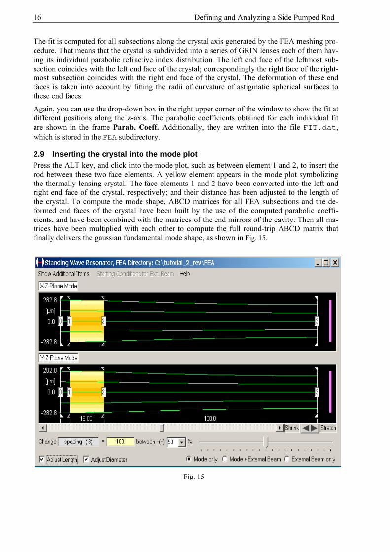
2.9 Inserting the crystal into the mode plot Press the ALT key, and click into the mode plot, such as between element 1 and 2, to insert the rod between these two face elements. A yellow element appears in the mode plot symbolizing the thermally lensing crystal. The face elements 1 and 2 have been converted into the left and right end face of the crystal, respectively; and their distance has been adjusted to the length of the crystal. To compute the mode shape, ABCD matrices for all FEA subsections and the de-formed end faces of the crystal have been built by the use of the computed parabolic coeffi-cients, and have been combined with the matrices of the end mirrors of the cavity. Then all ma-trices have been multiplied with each other to compute the full round-trip ABCD matrix that finally delivers the gaussian fundamental mode shape, as shown in Fig. 15.

Fig. 15

Analyzing stability of a laser cavity 17

3 Modifying cavity parameters To modify parameters of a resonator configuration, such as the cavity shown in Fig. 15, with a rod between two external mirrors, many tools are provided in LASCAD.

You can shrink and stretch the plot by the use of the two arrows immediately below the mode plot.

You can click on the end mirrors and move them with the mouse.

Also the yellow symbol for the crystal can be moved with the mouse.

To insert an additional element, press the SHIFT key, and click into the mode plot at a position where you would like to insert the element. The Insert Element window pops up, where you can define the type of the element, focal distance or radius of curvature etc. (see the manual or Tutorial No. 1 for additional information)

To clear an element, position the mouse pointer over the element, press the CTRL key, and then the left mouse button. The thermal lens can also be cleared in this way.

The curvature of the end mirrors can be modified by changing the entries in the related boxes in the row Type-Param., in the window Parameter Field.

Another way to change parameters works as follows: click into one of the boxes in the window Parameter Field, and then move the slider below the mode plot to change the related quantity, as described in the manual and in the Quick Tour.

To investigate dependence of the thermal lensing effect on the pump power, proceed as follows: click the tab Miscellaneous, in the window Parameter Field, and enter a new value into the box Pump power for rescaling. All thermal effects will be linearly rescaled corresponding to the ratio between original pump power and the value entered for rescaling.

Additional tools are described in the LASCAD manual.

4 Tools to analyze the properties of a laser cavity LASCAD is provides several tools to analyze the properties of the cavity. Some of them are explained below in context with the present example.

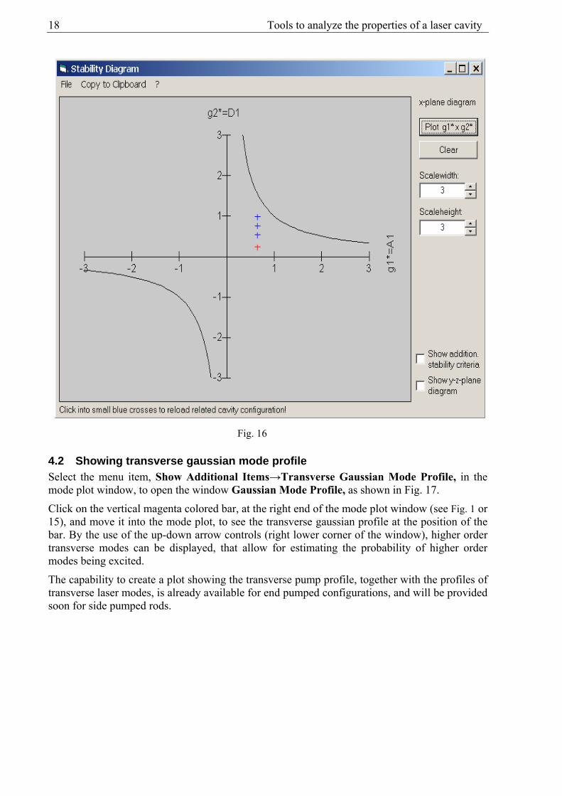
4.1 Analyzing stability of a laser cavity Select the menu item Show Additional Items→Stability Diagram, in the mode plot window, to open the window Stability Diagram, as shown in Fig. 16.

Click the button Plot g1* x g2* to show the stability of the actual resonator configuration. A red cross symbol is plotted, whose position within the diagram represents the stability of the cavity. If you are changing a cavity parameter, for instance the curvature of a mirror, click the button again to plot a second cross, whose position shows the influence of the parameter modification on the stability of the cavity. You can continue in this way and plot a series of crosses. The color of the latest one is always red, and the previously plotted crosses change to blue.

An important issue is the dependence of the cavity stability on the pump power. To analyze this, rescale the pump power, as described in section 3.

Check the box Show y-plane diagram, in the window Stability Diagram, to also show the stability diagram for the y-plane mode.

Theoretical explanations, such as the definition of the generalized g-parameters, can be found in the online help or in the manual sect. 6.5.

18 Tools to analyze the properties of a laser cavity

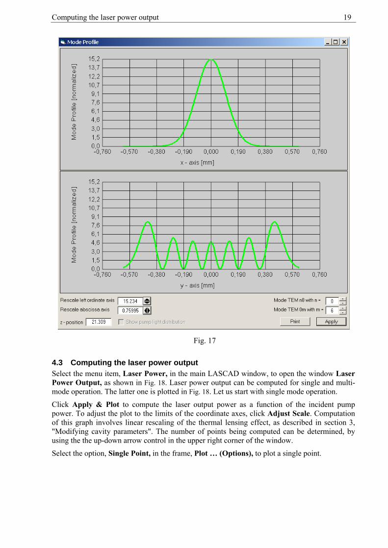
4.2 Showing transverse gaussian mode profile Select the menu item, Show Additional Items→Transverse Gaussian Mode Profile, in the mode plot window, to open the window Gaussian Mode Profile, as shown in Fig. 17.

Click on the vertical magenta colored bar, at the right end of the mode plot window (see Fig. 1 or 15), and move it into the mode plot, to see the transverse gaussian profile at the position of the bar. By the use of the up-down arrow controls (right lower corner of the window), higher order transverse modes can be displayed, that allow for estimating the probability of higher order modes being excited.

The capability to create a plot showing the transverse pump profile, together with the profiles of transverse laser modes, is already available for end pumped configurations, and will be provided soon for side pumped rods.

Fig. 16

Computing the laser power output 19

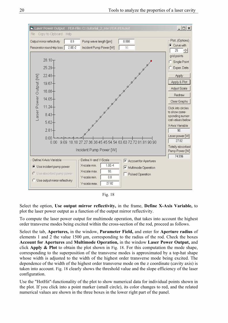
4.3 Computing the laser power output Select the menu item, Laser Power, in the main LASCAD window, to open the window Laser Power Output, as shown in Fig. 18. Laser power output can be computed for single and multi-mode operation. The latter one is plotted in Fig. 18. Let us start with single mode operation.

Click Apply & Plot to compute the laser output power as a function of the incident pump power. To adjust the plot to the limits of the coordinate axes, click Adjust Scale. Computation of this graph involves linear rescaling of the thermal lensing effect, as described in section 3, "Modifying cavity parameters". The number of points being computed can be determined, by using the the up-down arrow control in the upper right corner of the window.

Select the option, Single Point, in the frame, Plot … (Options), to plot a single point.

Fig. 17

20 Tools to analyze the properties of a laser cavity

Select the option, Use output mirror reflectivity, in the frame, Define X-Axis Variable, to plot the laser power output as a function of the output mirror reflectivity.

To compute the laser power output for multimode operation, that takes into account the highest order transverse modes being excited within the cross-section of the rod, proceed as follows.

Select the tab, Apertures, in the window, Parameter Field, and enter for Aperture radius of elements 1 and 2 the value 1500 μm, corresponding to the radius of the rod. Check the boxes Account for Apertures and Multimode Operation, in the window Laser Power Output, and click Apply & Plot to obtain the plot shown in Fig. 18. For this computation the mode shape, corresponding to the superposition of the transverse modes is approximated by a top-hat shape whose width is adjusted to the width of the highest order transverse mode being excited. The dependence of the width of the highest order transverse mode on the z coordinate (cavity axis) is taken into account. Fig. 18 clearly shows the threshold value and the slope efficiency of the laser configuration.

Use the "HotHit"-functionality of the plot to show numerical data for individual points shown in the plot. If you click into a point marker (small circle), its color changes to red, and the related numerical values are shown in the three boxes in the lower right part of the panel.

Fig. 18


Instead of checking Account for Apertures, the highest order transverse modes also can be defined directly by selecting the tab Miscellaneous, in the window Parameter Field, as shown in Fig. 19. Define beam qualities for x- and y-plane mode, or use the up-down arrow controls,

to define the highest transverse mode.

If Account for Apertures is checked without checking Multimode Operation, the apertures are used to confine the width of the fundamental mode only.

Pulsed operation is approximated by the use of rectangular pulses. Check the box Pulsed Op-eration to enter pulse length and frequency.

Multimode and pulsed operation can be computed much more accurately with the new DMA code, for dynamic analysis of multimode and Q-switch operation. See Tutorial No. 4.

5 The Beam Propagation Code (BPM) Parabolic approximation and ABCD matrix code are not always sufficient.

In these cases FEA results can alternatively be used as input for a physical optics beam propaga-tion code. This code provides full 3D simulation of the interaction of a propagating wave front with the hot, thermally deformed crystal, without using parabolic approximation. Here only a short instruction is given for startng the BPM code, using default parameter settings. For details the reader is referred to the manual.

To compute the fundamental mode shape, change the transverse mode order to zero in the tab Miscellaneous, in the Parameter Field window. Then select BPM→Run BPM, in the menu bar of the main LASCAD window, to open the window shown in Fig. 20. The entries of this window control the execution of the BPM code, and are described in detail in the manual.

Fig. 19

22 The Beam Propagation Code (BPM)

Fig. 20


An initial Beam profile can be defined that can be identical to the profile obtained by gaussian analysis, or can be a circular top hat profile with adjustable radius. To control the convergence of the BPM code, different types of apertures can be defined. To obtain convergence to the gaussian fundamental mode, it is useful to define apertures at the end mirrors, whose radii are twice the spot size of the gaussian fundamental.

To run the code in this way leave the default settings of the BPM input window unchanged, and click Run BPM to start the BPM code. Together, with the BPM main window, two graphics windows are opened. One of them dsiplays the mode profile at the right end mirror, as shown in Fig. 21. The other one shows the convergence of the beam radius with increasing cavity itera-tion, as shown in Fig. 22.

Fig. 21

24 The Beam Propagation Code (BPM)

The scale, Cavity Iteration, shows the number of full round trips of the wave front propagating back and forth between the mirrors.

The 1/e2 beam radius, shown in Fig. 22, converges very well to the gaussian spot size at the right mirror, as shown in Fig. 23. The large-scale fluctuations are caused by mode beating ef-fects of the fundamental mode with higher order transverse modes.

Fig. 22

Fig. 23


To obtain a multimode structure, check the option, The full computational window is used as aperture, in the frame Use of Apertures, as shown in Fig. 20. Then select, as initial beam pro-file, Circular top hat … (available only with full version) or Gaussian with spot size defined in the box below. Enter a radius slightly smaller than the half width of the computational win-dow. In addition, you can increase the latter one after unchecking the box, Use results of gaus-sian analysis to compute half width of computation window. An example for a multimode profile is shown in Fig. 24.

A detailed listing of numerical results created by the BPM code such as laser power output, beam quality, etc., can be found in the file lyra.txt, in the subdirectory BPM, of the LASCAD working directory. A user guide for the BPM code can be found in the file BPM user_guide.chm, in the subdirectory Documentation, of the LASCAD application directory.

Fig. 24

lascad tutorial no. 2: modeling a laser cavity with side ... · lascad tutorial no. 2: ... the...

Documents