LASCAD Tutorial No. 3: Modeling an Yb:YAG thin disk laser

Revised: January 19, 2009

© Copyright 2006 - 2009 LAS-CAD GmbH

Table of Contents 1

Table of Contents

1 Starting LASCAD and Defining Pump Light Distribution .........................................................3 2 Defining Boundary Conditions Used with FEA..........................................................................5 3 Defining Options to Control FEA................................................................................................6 4 Showing the FEA Results ............................................................................................................7 5 Creating a Parabolic Fit of the FEA Results................................................................................7 6 Inserting the Thermal Lens into the Mode Plot ...........................................................................8 7 Computing Laser Power Output ..................................................................................................9 8 The Beam Propagation Code (BPM).........................................................................................13

Note: The project file Tutorial_3.lcd of the example generated with this tutorial can be found in the directory Tutorials on the CD-ROM or after installation of LASCAD in the subdirectory Tutorials of the LASCAD application directory. You can copy this file to a working direc-tory and open it by double-click.

Starting LASCAD and Defining Pump Light Distribution 3

1 Starting LASCAD and Defining Pump Light Distribution • Start LASCAD and open Tutotial_3.lcd in the directory C:\Program

Files\LASCAD\Tutorials, • Define a working directory, • Stretch the mode plot, by the use of the "shrink-stretch" tool until you can see the yellow

symbol for the thermal lensing disc. Since the disc is only is 0.12 mm thick, you must stretch a lot,

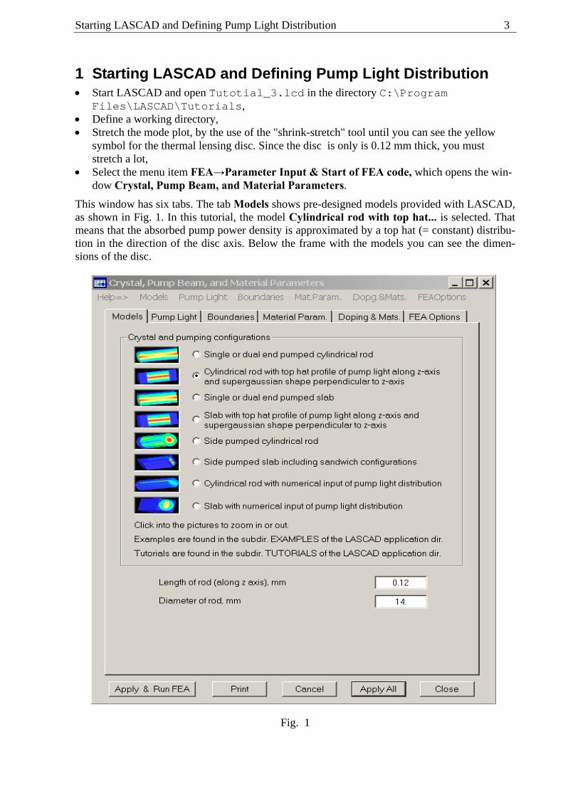
• Select the menu item FEA→Parameter Input & Start of FEA code, which opens the win-dow Crystal, Pump Beam, and Material Parameters.

This window has six tabs. The tab Models shows pre-designed models provided with LASCAD, as shown in Fig. 1. In this tutorial, the model Cylindrical rod with top hat... is selected. That means that the absorbed pump power density is approximated by a top hat (= constant) distribu-tion in the direction of the disc axis. Below the frame with the models you can see the dimen-sions of the disc.

Fig. 1

4

Select the tab Pump Light, as shown in Fig. 2, to define the absorbed pump power density. With this model you must know in advance the totally absorbed pump power. It has been as-sumed that 500 W are absorbed in the disc. The pump profile perpendicular to the axis of the disc can be defined by the use of supergaussian functions, as explained in the help=> menu item Pump Light→Top Hat Pump Light Distribution in Axis Direction, or in the manual. The spot size is the radius of the distribution. If the super-gaussian exponent is increased to a large number, the profile approaches top hat. Click the button Show Pump Profile to see the profile. You can even subtract a negative contribution from the profile, based on a percentage scale, related to the absorbed pump power.

Fig. 2

Defining Boundary Conditions Used with FEA 5

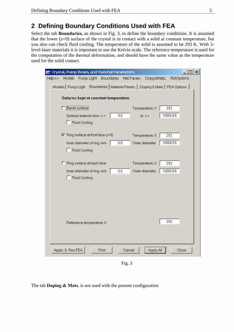
2 Defining Boundary Conditions Used with FEA Select the tab Boundaries, as shown in Fig. 3, to define the boundary conditions. It is assumed that the lower (z=0) surface of the crystal is in contact with a solid at constant temperature, but you also can check fluid cooling. The temperature of the solid is assumed to be 293 K. With 3-level-laser materials it is important to use the Kelvin scale. The reference temperature is used for the computation of the thermal deformation, and should have the same value as the temperature used for the solid contact.

The tab Doping & Mats. is not used with the present configuration

Fig. 3

6

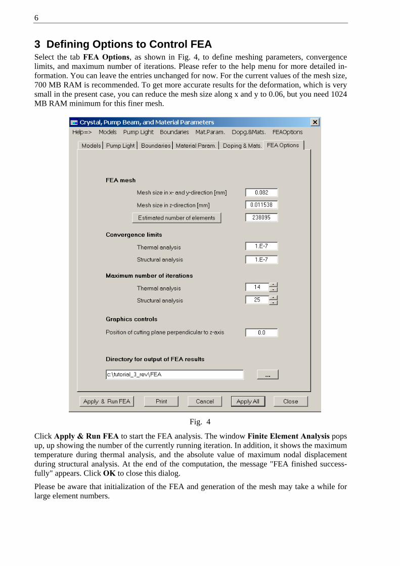
3 Defining Options to Control FEA Select the tab FEA Options, as shown in Fig. 4, to define meshing parameters, convergence limits, and maximum number of iterations. Please refer to the help menu for more detailed in-formation. You can leave the entries unchanged for now. For the current values of the mesh size, 700 MB RAM is recommended. To get more accurate results for the deformation, which is very small in the present case, you can reduce the mesh size along x and y to 0.06, but you need 1024 MB RAM minimum for this finer mesh.

Click Apply & Run FEA to start the FEA analysis. The window Finite Element Analysis pops up, up showing the number of the currently running iteration. In addition, it shows the maximum temperature during thermal analysis, and the absolute value of maximum nodal displacement during structural analysis. At the end of the computation, the message "FEA finished success-fully" appears. Click OK to close this dialog.

Please be aware that initialization of the FEA and generation of the mesh may take a while for large element numbers.

Fig. 4

Showing the FEA Results 7

4 Showing the FEA Results When the FEA is finished, click FEA→3D Visualizer, in the main LASCAD menu, to show results for heat load distribution, temperature distribution, deformation and stress. Fig. 5 shows the temperature distribution at the side of the disc that is not being cooled.

Click FEA→2D Data Profiles ... in the LASCAD menu to open the window 2D Profiles & Parabolic Fit, showing 2D plots of FEA results. By default, the temperature distribution is dis-played. Use the drop-down box in the upper right corner of this window to show 2D plots at different positions along the z-axis of the crystal, which correspond to FEA discretization points. Use the mouse wheel to scroll along the z axis.

5 Creating a Parabolic Fit of the FEA Results Click the button Refresh & Fit, in the window 2D Profiles & Parabolic Fit, to carry through a parabolic fit of the transverse refractive index distribution and the deformation. The fit is com-puted for a series of sections along the z axis, as generated by the FEA discretization. For the current meshing parameters, about 10 subsections have been created. The fit for the refractive index distribution is shown in Fig. 6.

Note that the fit is shown at z = 0.06 mm.

Fig. 5

8

Click the items Left face or Right Face, in the drop-down box Show Parab. Fit, to show the fit for the end faces. The results for the end faces are not accurate. Since the deformation is very small, you must use a finer mesh along x and y axis and run more iterations to get more accurate results. But this is not important for the present purpose, since the small deformation has almost no influence on the laser mode.

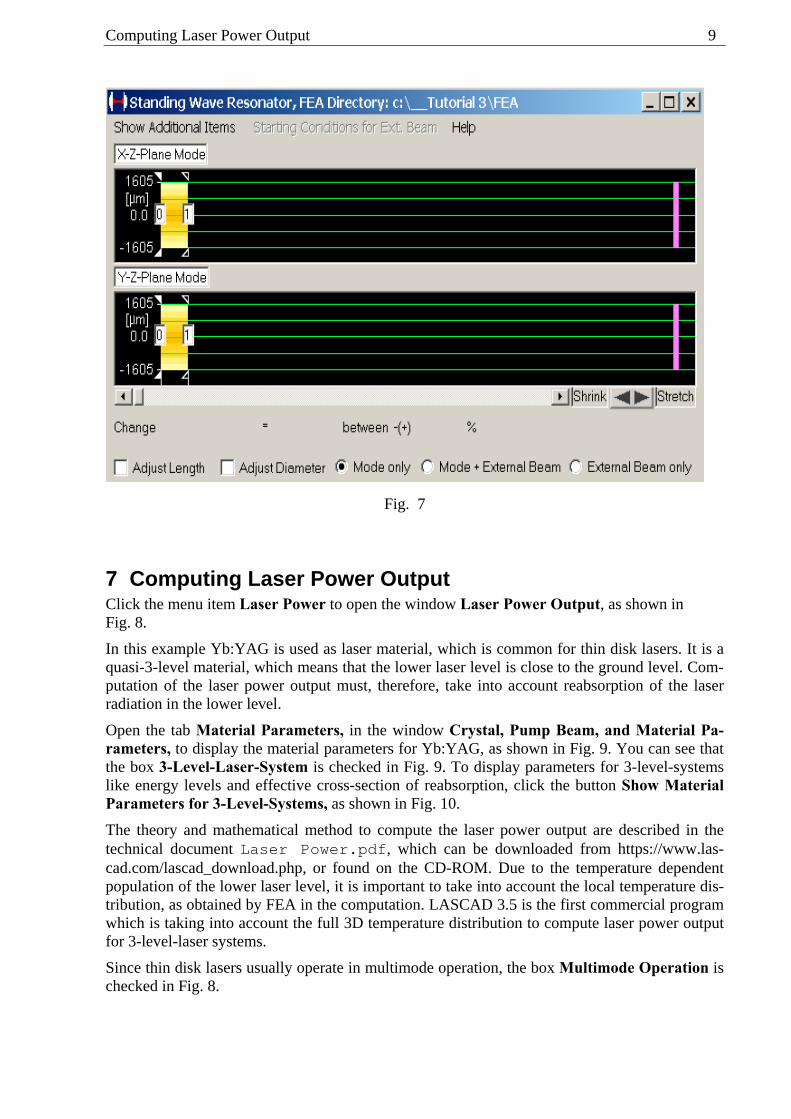
6 Inserting the Thermal Lens into the Mode Plot Press the ALT key, and click in the mode plot between element 0 and 1. You may have to stretch in advance. The yellow symbol for the thermal lens should appear, but since the length of the plot is adjusted to the width of the picture box immediately after insertion, you must stretch the plot again to display the thermal lens as shown in Fig. 7.

Fig. 6

Computing Laser Power Output 9

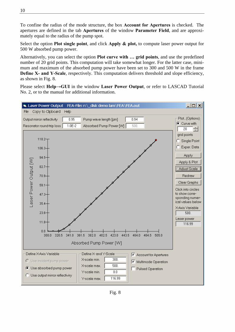
7 Computing Laser Power Output Click the menu item Laser Power to open the window Laser Power Output, as shown in Fig. 8.

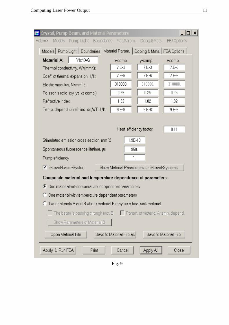
In this example Yb:YAG is used as laser material, which is common for thin disk lasers. It is a quasi-3-level material, which means that the lower laser level is close to the ground level. Com-putation of the laser power output must, therefore, take into account reabsorption of the laser radiation in the lower level.

Open the tab Material Parameters, in the window Crystal, Pump Beam, and Material Pa-rameters, to display the material parameters for Yb:YAG, as shown in Fig. 9. You can see that the box 3-Level-Laser-System is checked in Fig. 9. To display parameters for 3-level-systems like energy levels and effective cross-section of reabsorption, click the button Show Material Parameters for 3-Level-Systems, as shown in Fig. 10.

The theory and mathematical method to compute the laser power output are described in the technical document Laser Power.pdf, which can be downloaded from https://www.las-cad.com/lascad_download.php, or found on the CD-ROM. Due to the temperature dependent population of the lower laser level, it is important to take into account the local temperature dis-tribution, as obtained by FEA in the computation. LASCAD 3.5 is the first commercial program which is taking into account the full 3D temperature distribution to compute laser power output for 3-level-laser systems.

Since thin disk lasers usually operate in multimode operation, the box Multimode Operation is checked in Fig. 8.

Fig. 7

10

To confine the radius of the mode structure, the box Account for Apertures is checked. The apertures are defined in the tab Apertures of the window Parameter Field, and are approxi-mately equal to the radius of the pump spot.

Select the option Plot single point, and click Apply & plot, to compute laser power output for 500 W absorbed pump power.

Alternatively, you can select the option Plot curve with … grid points, and use the predefined number of 20 grid points. This computation will take somewhat longer. For the latter case, mini-mum and maximum of the absorbed pump power have been set to 300 and 500 W in the frame Define X- and Y-Scale, respectively. This computation delivers threshold and slope efficiency, as shown in Fig. 8.

Please select Help→GUI in the window Laser Power Output, or refer to LASCAD Tutorial No. 2, or to the manual for additional information.

Fig. 8

Computing Laser Power Output 11

Fig. 9

12

Fig. 10

The Beam Propagation Code (BPM) 13

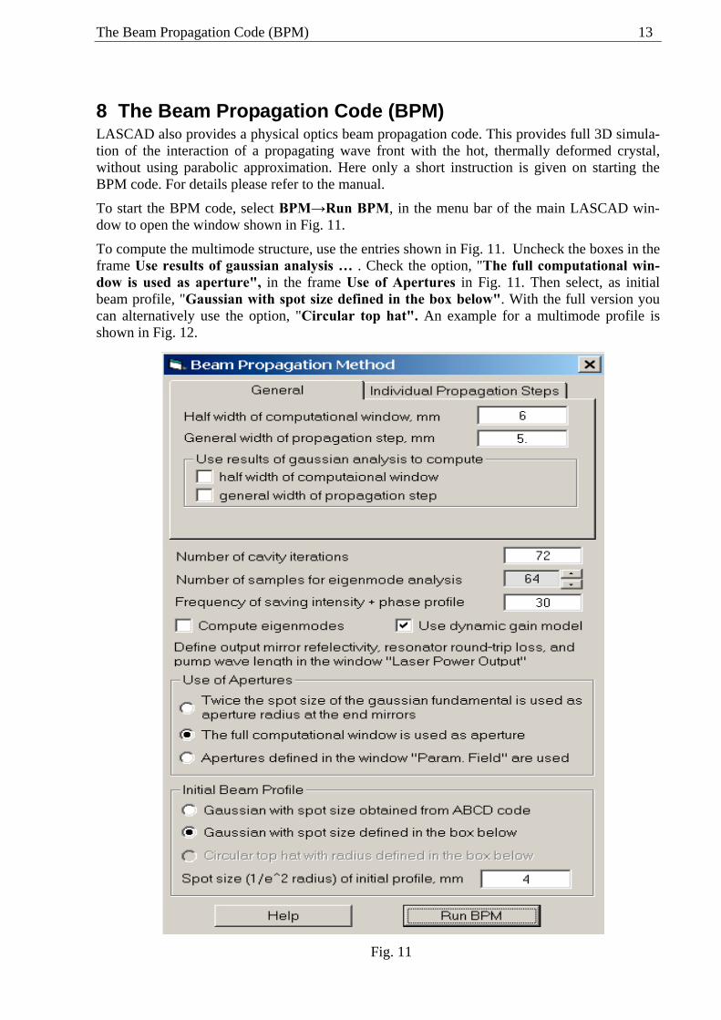
8 The Beam Propagation Code (BPM) LASCAD also provides a physical optics beam propagation code. This provides full 3D simula-tion of the interaction of a propagating wave front with the hot, thermally deformed crystal, without using parabolic approximation. Here only a short instruction is given on starting the BPM code. For details please refer to the manual.

To start the BPM code, select BPM→Run BPM, in the menu bar of the main LASCAD win-dow to open the window shown in Fig. 11.

To compute the multimode structure, use the entries shown in Fig. 11. Uncheck the boxes in the frame Use results of gaussian analysis … . Check the option, "The full computational win-dow is used as aperture", in the frame Use of Apertures in Fig. 11. Then select, as initial beam profile, "Gaussian with spot size defined in the box below". With the full version you can alternatively use the option, "Circular top hat". An example for a multimode profile is shown in Fig. 12.

Fig. 11

14

A detailed listing of numerical results created by the BPM code, such as laser power output, beam quality etc. can be found in the file lyra.txt in the subdirectory BPM of the LASCAD working directory. A user guide for the BPM code can be found in the file BPM user_guide.chm, in the subdirectory Documentation of the LASCAD application directory.

Fig. 12