last study topics value vs growth stock standard vs consumption capm asset pricing model three...
TRANSCRIPT
Last Study Topics
• Value Vs Growth Stock• Standard vs Consumption CAPM• Asset Pricing Model• Three Factor Model

Today’s Study Topics
• Understanding of Statements• Qualification of Statements• Numerical

True or false?
• Explain or qualify as necessary.• a. Investors demand higher expected rates of
return on stocks with more variable rates of return.

True or false?
• Explain or qualify as necessary.• a. Investors demand higher expected rates of
return on stocks with more variable rates of return.
– False – investors demand higher expected rates of return on stocks with more non-diversifiable risk.

Continue
• b. The CAPM predicts that a security with a beta of 0 will offer a zero expected return.

Continue
• b. The CAPM predicts that a security with a beta of 0 will offer a zero expected return.
– False – a security with a beta of zero will offer the risk-free rate of return.

Continue
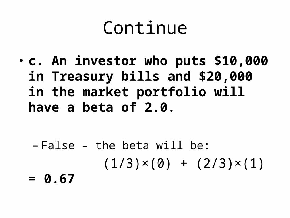
• c. An investor who puts $10,000 in Treasury bills and $20,000 in the market portfolio will have a beta of 2.0.
Continue
• c. An investor who puts $10,000 in Treasury bills and $20,000 in the market portfolio will have a beta of 2.0.
– False – the beta will be:
(1/3)×(0) + (2/3)×(1) = 0.67
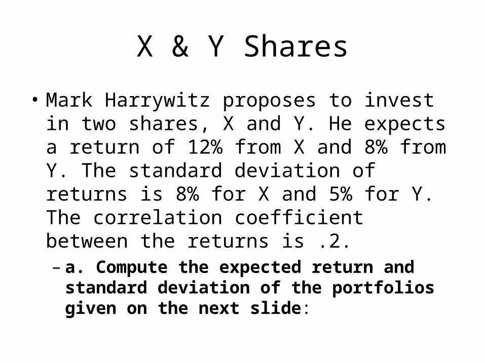
X & Y Shares
• Mark Harrywitz proposes to invest in two shares, X and Y. He expects a return of 12% from X and 8% from Y. The standard deviation of returns is 8% for X and 5% for Y. The correlation coefficient between the returns is .2.– a. Compute the expected return and standard
deviation of the portfolios given on the next slide:

Continue
PortfoliosPORTFOLIO % IN X % IN Y
1 50 50
2 25 75
3 75 25
Solutions:PORTFOLIO Mean (r) S.D
1 10% 5.1%
2 9.0% 4.6%
3 11.0% 6.4%

Graph• b. Sketch the set of
portfolios composed of X and Y.
Solution: The set of portfolios is
represented by the curved line. The five points are the three portfolios from Part
(a) plus the two following two
portfolios: -One consists of 100% invested in X and the
other consists of 100% invested in Y.

Shares Investment
• Example: M. Grandet has invested 60 percent of his money in share A and the remainder in share B. He assesses their prospects as follows:
A B
Expected Return % 15 20
Standard Deviation % 20 22
Correlation .5 .5

Continue
• a. What are the expected return and standard deviation of returns on his portfolio?
– Expected return = (0.6 × 15) + (0.4 × 20) = 17%– Variance = (0.6)2 ×(20)2 + (0.4)2 × (22)2 + 2(0.6)
(0.4)(0.5)(20)(22) = 327– Standard deviation = (327)(1/2) = 18.1%
Continue
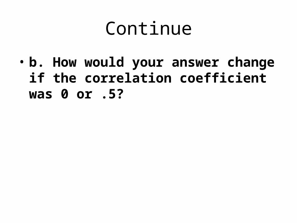
• b. How would your answer change if the correlation coefficient was 0 or .5?

Continue
• b. How would your answer change if the correlation coefficient was 0 or .5?
– Correlation coefficient = 0 Standard deviation = ⇒14.9%
– Correlation coefficient = -0.5 Standard ⇒deviation = 10.8%
Continue
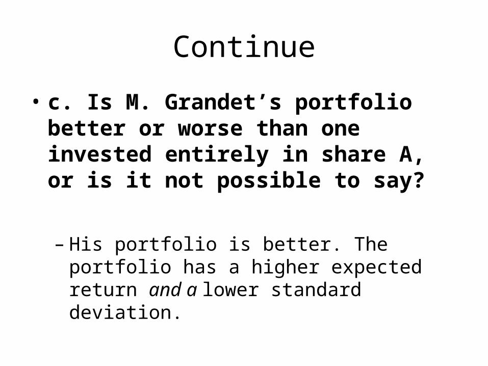
• c. Is M. Grandet’s portfolio better or worse than one invested entirely in share A, or is it not possible to say?
– His portfolio is better. The portfolio has a higher expected return and a lower standard deviation.

Case: Percival Hygiene • Percival Hygiene has $10 million invested in
long-term corporate bonds. This bond portfolio’s expected annual rate of return is 9%, and the annual standard deviation is 10%.
• Amanda Reckonwith, Percival’s financial adviser, recommends that Percival consider investing in an index fund which closely tracks the Standard and Poor’s 500 index. The index has an expected return of 14%, and its standard deviation is 16%.

Required (a)
• a. Suppose Percival puts all his money in a combination of the index fund and Treasury bills. – Can he thereby improve his expected rate of
return without changing the risk of his portfolio? The Treasury bill yield is 6%.

Understanding
• Percival’s current portfolio provides an expected return of 9% with an annual standard deviation of 10%.
• First we find the portfolio weights for a combination of Treasury bills (security 1: standard deviation = 0%) and the index fund (security 2: standard deviation = 16%) such that portfolio standard deviation is 10%.

Continue• In general, for a two security portfolio:
• Further:
– Therefore, he can improve his expected rate of return without changing the risk of his portfolio.

Summary
• Understanding of Statements• Qualification of Statements• Numerical

Continue
• b. Could Percival do even better by investing equal amounts in the corporate bond portfolio and the index fund? – The correlation between the bond portfolio and
the index fund is +0.1.– rp = x1r1 + x2r2– rp = (0.5 × 0.09) + (0.5 × 0.14) = 0.115 = 11.5%

Continue
• σP2 = x1
2σ12 + 2x1x2σ1σ2ρ12 + x2
2σ22
• σP 2 = (0.5)2(0.10)2 + 2(0.5)(0.5)(0.10)(0.16)(0.10) + (0.5)2(0.16)2
• σP2 = 0.0097
• σP = 0.985 = 9.85%

Understanding
• Therefore, he can do even better by investing equal amounts in the corporate bond portfolio and the index fund.
• His expected return increases to 11.5% and the standard deviation of his portfolio decreases to 9.85%.

Explain• “There may be some truth in these CAPM and
APT theories, but last year some stocks did much better than these theories predicted, and other stocks did much worse.” Is this a valid criticism?
– No. Every stock has unique risk in addition to market risk. The unique risk reflects uncertain events that are unrelated to the return on the market portfolio. The Capital Asset Pricing Model does not predict these events.

Explain
• a. The APT factors cannot reflect diversifiable risks.– True. By definition, the factors represent macro-
economic risks that cannot be eliminated by diversification.
• b. The market rate of return cannot be an APT factor.– False. The APT does not specify the factors.

Continue
• c. Each APT factor must have a positive risk premium associated with it; otherwise the model is inconsistent.
– True. Investors will not take on non-diversifiable risk unless it entails a positive risk premium.
Continue
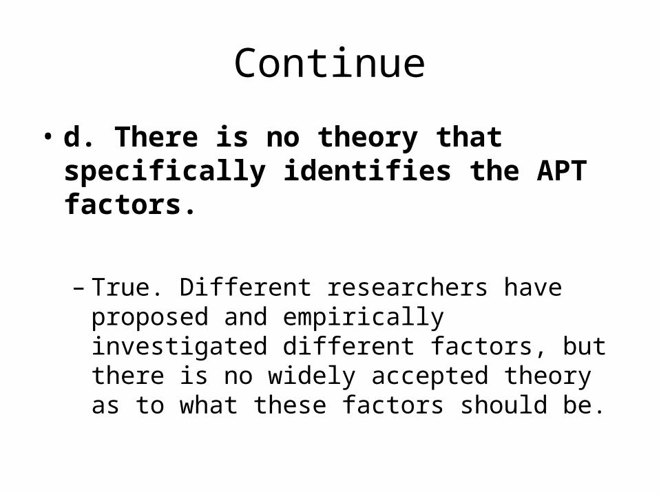
• d. There is no theory that specifically identifies the APT factors.
– True. Different researchers have proposed and empirically investigated different factors, but there is no widely accepted theory as to what these factors should be.

Continue
• e. The APT model could be true but not very useful, for example, if the relevant factors change unpredictably.
– True. To be useful, we must be able to estimate the relevant parameters.
– If this is impossible, for whatever reason, the model itself will be of theoretical interest only.

APT Model– Consider the following simplified APT model:
Factor Risk Exposures
FACTOR EXPECTED RISK PREMIUM
Market 6.4%
Interest rate -0.6%
Yield Spread 5.1%
MARKET INTEREST RATE YIELD SPREAD
STOCK (b1) (b2) (b3)
P 1.0 -2.0 -0.2
P2 1.2 0 .3
P3 .3 .5 1.0

Continuea. Calculate the expected return for the
following stocks. Assume rf = 5%.– For Stock P r = (1.0)×(6.4%) + (-2.0)×(-0.6%) + ⇒
(-0.2)×(5.1%) = 6.58%
– For Stock P2 r = (1.2)×(6.4%) + (0)×(-0.6%) + ⇒(0.3)×(5.1%) = 9.21%
– For Stock P3 r = (0.3)×(6.4%) + (0.5)×(-0.6%) + ⇒(1.0)×(5.1%) = 6.72%

Continue
• b. What are the factor risk exposures for the portfolio?– Factor risk exposures:
• b1(Market) = (1/3)×(1.0) + (1/3)×(1.2) + (1/3)×(0.3) = 0.83
• b2(Interest rate) = (1/3)×(-2.0) +(1/3)×(0) + (1/3)×(0.5) = -0.50
• b3(Yield spread) = (1/3)×(-0.2) + (1/3)×(0.3) + (1/3)×(1.0) = 0.37
Continue
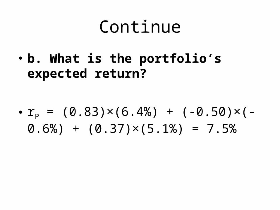
• b. What is the portfolio’s expected return?
• rP = (0.83)×(6.4%) + (-0.50)×(-0.6%) + (0.37)×(5.1%) = 7.5%

Three Factors Model
• The following table shows the sensitivity of four stocks to the three Fama–French factors in the five years to 2001. Estimate the expected return on each stock assuming that the interest rate is 3.5%, the expected risk premium on the market is 8.8%, the expected risk premium on the size factor is 3.1%, and the expected risk premium on the book-to-market factor is 4.4%.

ContinueFactor Sensitivities
FACTOR COCA-COLA EXXON MOBILE PFIZER REEBOK
Market .82 .50 .66 1.17
Size -0.29 .04 -.56 .73
Book-to-Market
.24 .27 -.07 1.14
rCoca-Cola = 3.5% + (0.82 × 8.8%) + (-0.29 × 3.1%) + (0.24 × 4.4%) = 10.87%rEXXON= 3.5% + (0.50 × 8.8%) + (0.04 × 3.1%) + (0.27 × 4.4%) = 9.21%
Continue
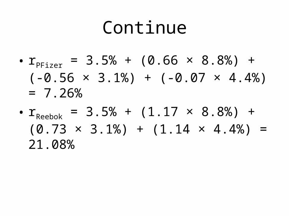
• rPFizer = 3.5% + (0.66 × 8.8%) + (-0.56 × 3.1%) + (-0.07 × 4.4%) = 7.26%
• rReebok = 3.5% + (1.17 × 8.8%) + (0.73 × 3.1%) + (1.14 × 4.4%) = 21.08%

Principles of Corporate
Finance
Sixth Edition
Richard A. Brealey
Stewart C. Myers
Chapter 9
McGraw Hill/Irwin
Capital Budgeting and Risk

Topics Covered
• Company and Project Costs of Capital• Measuring the Cost of Equity• Capital Structure and COC• Discount Rates for Intl. Projects• Estimating Discount Rates• Risk and DCF
Introduction
• LONG BEFORE THE development of modern theories linking risk and expected return, smart financial managers adjusted for risk in capital budgeting.
• How they should treat the element of risk with respect to each and every projects of different class?

Continue
• Various rules of thumb are often used to make these risk adjustments. – For example, many companies estimate the rate
of return required by investors in their securities and then use this company cost of capital to discount the cash flows on new projects.
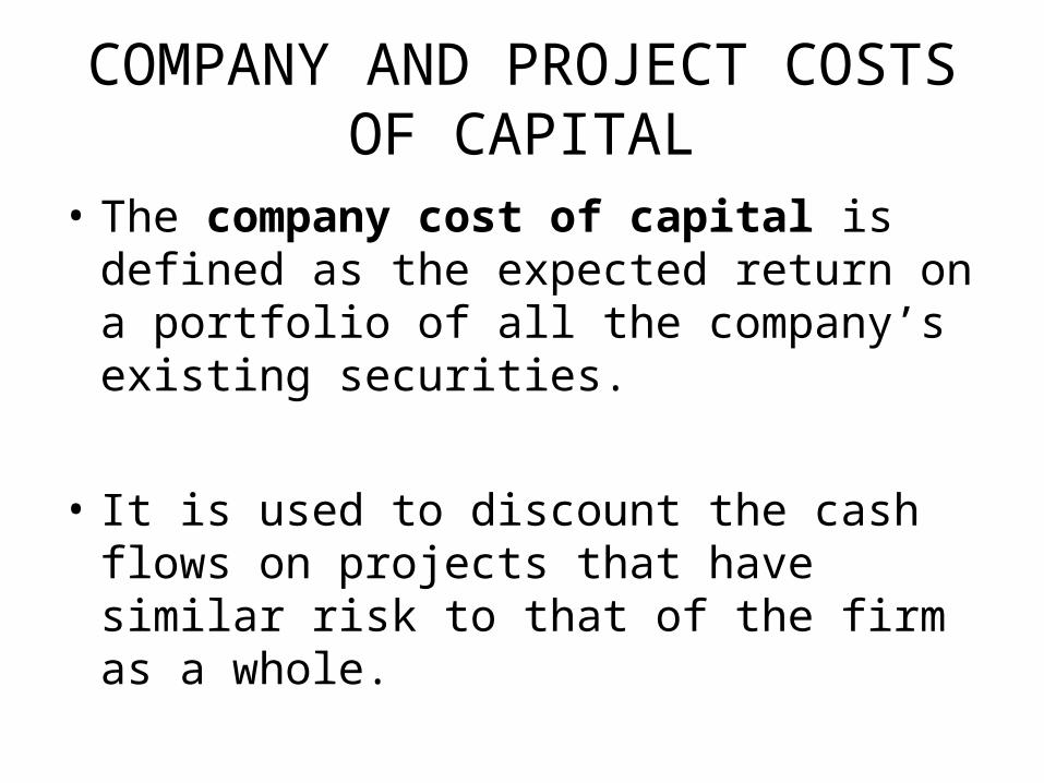
COMPANY AND PROJECT COSTS OF CAPITAL
• The company cost of capital is defined as the expected return on a portfolio of all the company’s existing securities.
• It is used to discount the cash flows on projects that have similar risk to that of the firm as a whole.

Continue
• We estimated that investors require a return of 9.2% from Pfizer common stock.
• If Pfizer is contemplating an expansion of the firm’s existing business, it would make sense to discount the forecasted cash flows at 9.2 %.
• The company cost of capital is not the correct discount rate if the new projects are more or less risky than the firm’s existing business..

Company Cost of Capital
• A firm’s value can be stated as the sum of the value of its various assets.
• Each project should in principle be evaluated at its own opportunity cost of capital.
• For a firm composed of assets A and B, the firm value is;
PV(B)PV(A)PV(AB) valueFirm

Continue• Here PV(A) and PV(B) are valued just as if they
were mini-firms in which stockholders could invest directly.
• Investors would value A by discounting its forecasted cash flows at a rate reflecting the risk of A.
• They would value B by discounting at a rate reflecting the risk of B. – The two discount rates will, in general, be
different.
Continue
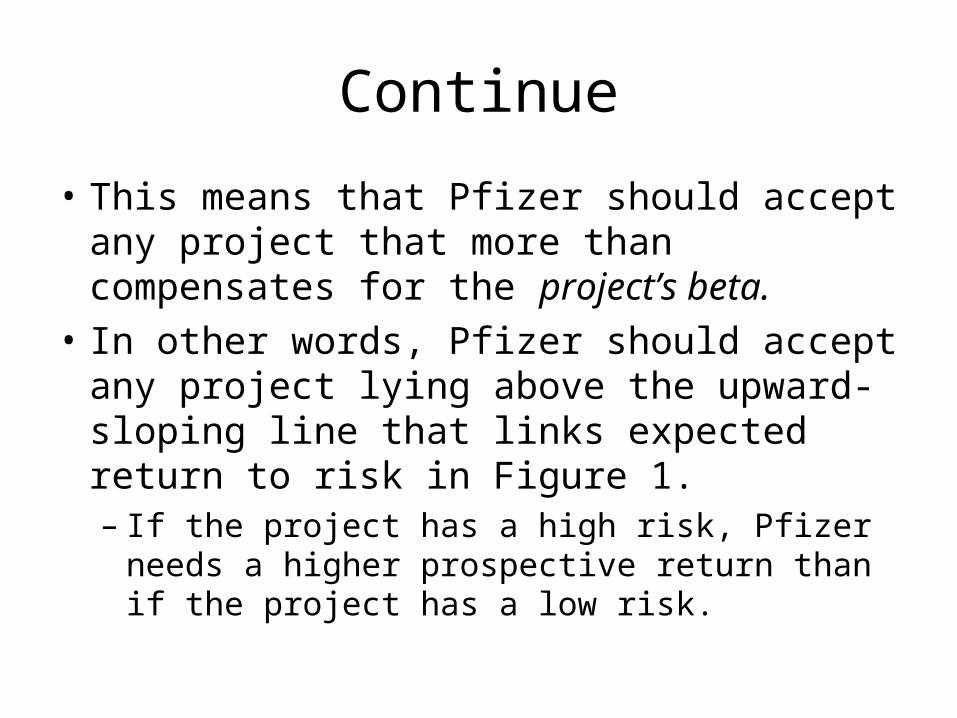
• This means that Pfizer should accept any project that more than compensates for the project’s beta.
• In other words, Pfizer should accept any project lying above the upward-sloping line that links expected return to risk in Figure 1. – If the project has a high risk, Pfizer needs a higher
prospective return than if the project has a low risk.
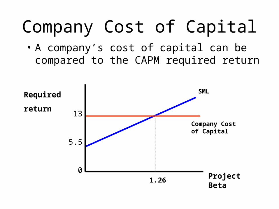
Company Cost of Capital• A company’s cost of capital can be compared
to the CAPM required return
Required
return
Project Beta1.26
Company Cost of Capital
13
5.5
0
SML

Understanding
• In terms of Figure1, the rule tells Pfizer to accept any project above the horizontal cost of capital line, that is, any project offering a return of more than 9.2%.– The company cost of capital rule, which is to
accept any project regardless of its risk as long as it offers a higher return than the company’s cost of capital.

Understanding
– It is clearly silly to suggest that Pfizer should demand the same rate of return from a very safe project as from a very risky one.
– If Pfizer used the company cost of capital rule, it would reject many good low-risk projects and accept many poor high-risk projects.
• Many firms require different returns from different categories of investment.

Understanding
10%nologyknown tech t,improvemenCost
COC)(Company 15%business existing ofExpansion
20%products New
30% ventureseSpeculativ
RateDiscount Category
For example, discount rates might be set as follows:

Perfect Pitch and the Cost of Capital• The true cost of capital depends on project
risk, not on the company undertaking the project. – So why is so much time spent estimating the
company cost of capital?
• First, many (maybe, most) projects can be treated as average risk, that is, no more or less risky than the average of the company’s other assets.– For these projects the company cost of capital is
the right discount rate.

Continue
• Second, the company cost of capital is a useful starting point for setting discount rates for unusually risky or safe projects. – It is easier to add to, or subtract from, the
company cost of capital than to estimate each project’s cost of capital from scratch.
• Anyone who can carry a tune gets relative pitches right.

Business People
• are used to, but not about absolute risk or required rates of return.
• Therefore, they set a companywide cost of capital as a benchmark.
• This is not the right hurdle rate for everything the company does.– But adjustments can be made for more or less
risky ventures.

MEASURING THE COST OF EQUITY
• Suppose that you are considering an across-the-board expansion by your firm.
• Such an investment would have about the same degree of risk as the existing business.
• Therefore you should discount the projected flows at the company cost of capital.
• Companies generally start by estimating the return that investors require from the company’s common stock.

Continue
• Used the capital asset pricing model to do the working. This states;– Expected stock return =rf + Beta(rm – rf)
• An obvious way to measure the beta (B) of a stock is to look at how its price has responded in the past to market movements.

Measuring Betas
• The SML shows the relationship between return and risk.
• CAPM uses Beta as a proxy for risk.• Other methods can be employed to determine
the slope of the SML and thus Beta.• Regression analysis can be used to find Beta.

Dell Computer Stock
• Calculated monthly returns from Dell Computer stock in the period, after it went public in 1988, is given on the next slide.
• Also plotted returns against the market returns for the same month, is given too.
• We have fitted a line through the points. – The slope of this line is an estimate of beta.

Measuring BetasDell Computer
Slope determined from plotting the line of best fit.
Price data – Aug 88- Jan 95
Market return (%)
Dell return (%
)
R2 = .11
B = 1.62

Measuring BetasDell Computer
Slope determined from plotting the line of best fit.
Price data – Feb 95 – Jul 01
Market return (%)
Dell return (%
)
R2 = .27
B = 2.02

Other Stocks
• The next diagram shows a similar plot for the returns on General Motors stock, and the
• Third shows a plot for Exxon Mobil. • In each case we have fitted a line through the
points. • The slope of this line is an estimate of beta.
– It tells us how much on average the stock price changed for each additional 1% change in the market index.

Measuring BetasGeneral Motors
Slope determined from plotting the line of best fit.
Price data – Aug 88- Jan 95
Market return (%)
GM
return (%)
R2 = .13
B = 0.80
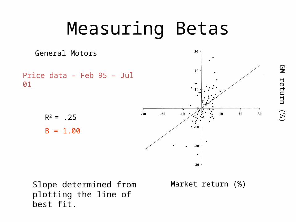
Measuring BetasGeneral Motors
Slope determined from plotting the line of best fit.
Price data – Feb 95 – Jul 01
Market return (%)
GM
return (%)
R2 = .25
B = 1.00

Measuring BetasExxon Mobil
Slope determined from plotting the line of best fit.
Price data – Aug 88- Jan 95
Market return (%)
Exxon Mobil return (%
)
R2 = .28
B = 0.52

Measuring BetasExxon Mobil
Slope determined from plotting the line of best fit.
Price data – Feb 95 – Jul 01
Market return (%)
Exxon Mobil return (%
)
R2 = .16
B = 0.42

Understanding• Diagrams show plots for the three stocks
during the subsequent period, February 1995 to July 2001.
• Although the slopes varied from the first period to the second, there is little doubt that Exxon Mobil’s beta is much less than Dell’s or that GM’s beta falls somewhere between the two. – If you had used the past beta of each stock to
predict its future beta, you wouldn’t have been too far off.
Understanding
• Only a small portion of each stock’s total risk comes from movements in the market.
• The rest is unique risk, which shows up in the scatter of points around the fitted
• lines in Diagrams. – R-squared (R2) measures the proportion of the
total variance in the stock’s returns that can be explained by market movements.
Table 1
Estimated betas and costs of (equity) capital for a sample of large railroad companies and for a portfolio of these companies. The precision of the portfolio beta is much better than that of the betas of the individual companies—note the lower standard error for the portfolio.

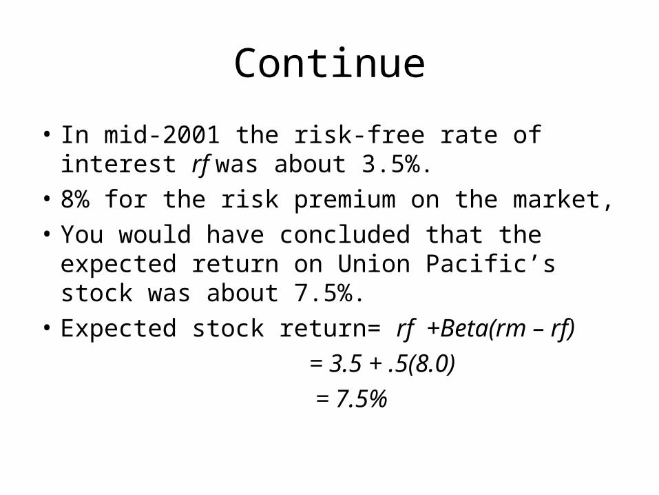
The Expected Return on Union Pacific Corporation’s Common Stock
• Suppose that in mid-2001 you had been asked to estimate the company cost of capital of Union Pacific Corporation.
• Table 1 provides two clues about the true beta
• of Union Pacific’s stock: – The direct estimate of .40 and the average
estimate for the industry of .50. • Use the industry average of .50
Continue
• In mid-2001 the risk-free rate of interest rf was about 3.5%.
• 8% for the risk premium on the market, • You would have concluded that the expected
return on Union Pacific’s stock was about 7.5%.• Expected stock return= rf +Beta(rm – rf) = 3.5 + .5(8.0) = 7.5%

CAPITAL STRUCTURE AND THE COMPANY COST OF CAPITAL
• we need to look at the relationship between the cost of capital and the mix of debt and equity used to finance the company.
• Think again of what the company cost of capital is and what it is used for.
• We define it as the opportunity cost of capital for the firm’s existing assets; – we use it to value new assets that have the same
risk as the old ones.

Company Cost of Capitalsimple approach
• Company Cost of Capital (COC) is based on the average beta of the assets
• The average Beta of the assets is based on the % of funds in each asset

Company Cost of Capitalsimple approach
Company Cost of Capital (COC) is based on the average beta of the assets
The average Beta of the assets is based on the % of funds in each asset
Example1/3 New Ventures B=2.01/3 Expand existing business B=1.31/3 Plant efficiency B=0.6
AVG B of assets = 1.3

Capital Structure
Capital Structure - the mix of debt & equity within a company
Expand CAPM to include CS
R = rf + B ( rm - rf )becomes
Requity = rf + B ( rm - rf )

Capital Structure & COC
COC = rportfolio = rassets
rassets = WACC = rdebt (D) + requity (E)
(V) (V)
Bassets = Bdebt (D) + Bequity (E)
(V) (V) requity = rf + Bequity ( rm - rf )

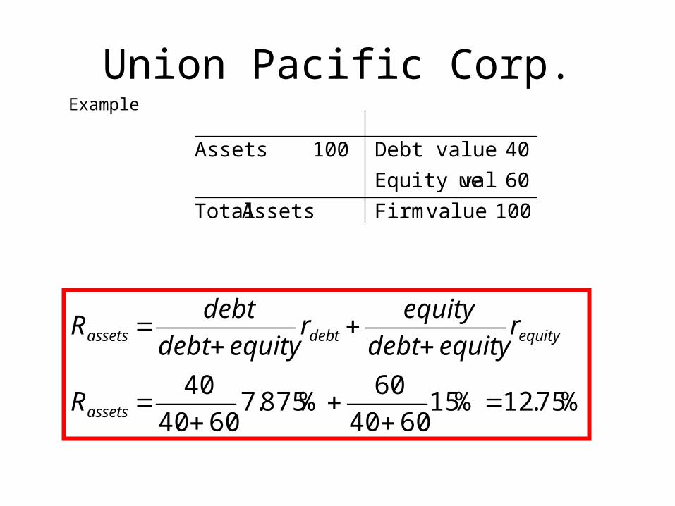
Union Pacific Corp.Example
100 valueFirmAssets Total
70ueEquity val
30Debt value100Assets
%75.12%157030
70%5.7
7030
30
assets
equitydebtassets
R
requitydebt
equityr
equitydebt
debtR

Understanding
• If the firm is contemplating investment in a project that has the same risk as the firm’s existing business, the opportunity cost of capital for this project is the same as the firm’s cost of capital; in other words, it is 12.75 percent.– What would happen if the firm issued an
additional 10 of debt and used the cash to repurchase 10 of its equity?
Union Pacific Corp.Example
100 valueFirmAssets Total
60ueEquity val
40Debt value100Assets
%75.12%156040
60%875.7
6040
40
assets
equitydebtassets
R
requitydebt
equityr
equitydebt
debtR

Understanding
• The change in financial structure does not affect the amount or risk of the cash flows on the total package of debt and equity.
• Therefore, if investors required a return of 12.75% on the total package before the refinancing, they must require a 12.75% return on the firm’s assets afterward.

Solve for Equity
• Since the company has more debt than before, the debt holders are likely to demand a higher interest rate.
• We will suppose that the expected return on the debt rises to 7.875%. – Now you can write down the basic equation for
the return on assets and solve for return on Equity. i.e.

Continue
• Return on equity = 16%– Increasing the amount of debt increased debtholder risk
and led to a rise in the return that debtholders required (rdebt rose from 7.5 to 7.875%). The higher leverage also made the equity riskier and increased the return that shareholders required (requity rose from 15 to 16 %).
equitydebtassets requitydebt
equityr
equitydebt
debtR
Continue
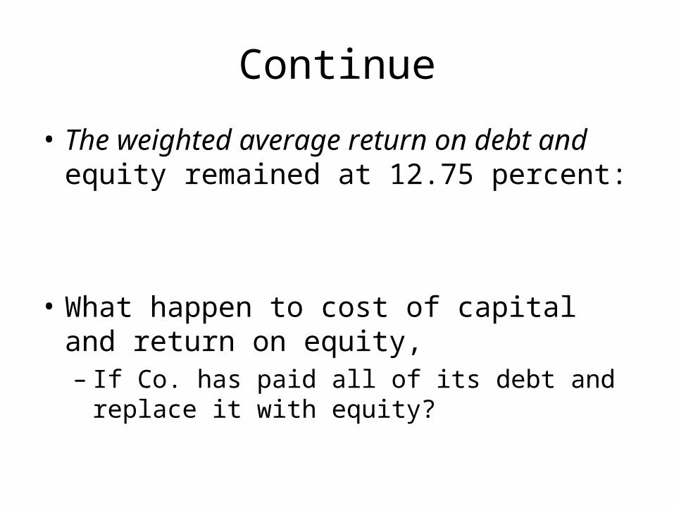
• The weighted average return on debt and equity remained at 12.75 percent:
• What happen to cost of capital and return on equity, – If Co. has paid all of its debt and replace it with
equity?

How Changing Capital Structure Affects Beta
• The stockholders and debtholders both receive a share of the firm’s cash flows, and both bear part of the risk. – For example, if the firm’s assets turn out to be
worthless, there will be no cash to pay stockholders or debtholders.
• But debtholders usually bear much less risk than stockholders. Debt betas of large blue-chip firms are typically in the range of .1 to .3.

Continue
• The firm’s asset beta is equal to the beta of a portfolio of all the firm’s debt and its equity.
• The beta of this hypothetical portfolio is just a weighted average of the debt and equity betas:
equitydebtassets Bequitydebt
equityB
equitydebt
debtB

Continue
• If the debt before the refinancing has a beta of .1 and the equity has a beta of 1.1, then;
• Beta assets = .8
equitydebtassets Bequitydebt
equityB
equitydebt
debtB

Continue
• What happens after the refinancing? The risk of the total package is unaffected, but both the debt and the equity are now more risky.– Suppose that the debt beta increases to 0.2.– Beta Equity = 1.2
equitydebtassets Bequitydebt
equityB
equitydebt
debtB

Understanding• Financial leverage does not affect the risk or
the expected return on the firm’s assets, but it does push up the risk of the common stock.
• Shareholders demand a correspondingly higher return because of this financial risk.
• Figure on the next slide shows the expected return and beta of the firm’s assets. – It also shows how expected return and risk are
shared between the debtholders and equity holders before the refinancing.

Capital Structure & COC
Expected return (%)
Bdebt Bassets Bequity
Rrdebt=7.5
Rassets=12.75
Requity=15
Expected Returns and Betas prior to refinancing
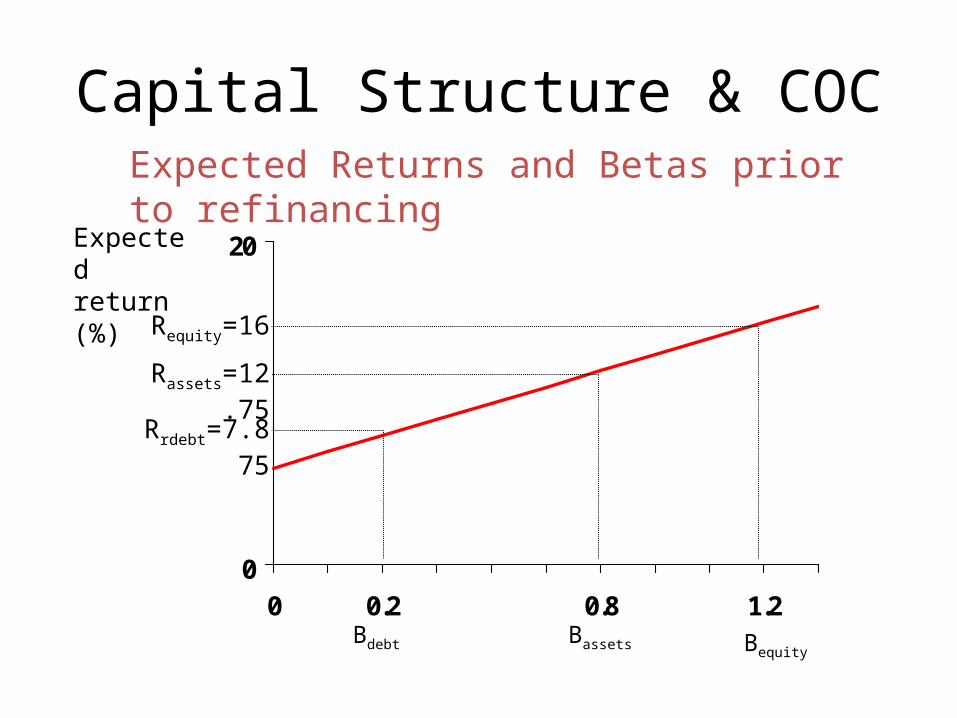
0
20
0 0.2 0.8 1.2
Capital Structure & COC
Expected return (%)
Bdebt Bassets Bequity
Rrdebt=7.875
Rassets=12.75
Requity=16
Expected Returns and Betas prior to refinancing

Summary

Union Pacific Corp.
Requity = Return on Stock
= 15%
Rdebt = YTM on bonds
= 7.5 %

Union Pacific Corp.
.17.50PortfolioIndustry
.21.40PacificUnion
.26.52SouthernNorfolk
.24.46tionTransporta CSX
.20.64Northern Burlington
Error Standard.Beta

International Risk
0.77.302.58Venezuela
1.39.482.91Thailand
0.81.421.93Poland
0.55.183.11Egypt
Betatcoefficien
nCorrelatioRatio
Source: The Brattle Group, Inc.
Ratio - Ratio of standard deviations, country index vs. S&P composite index

Asset Betas
)PV(revenue
PV(asset)B
)PV(revenue
cost) ePV(variablB
)PV(revenue
cost) PV(fixedBB
assetcost variable
cost fixedrevenue
)PV(revenue
PV(asset)B
)PV(revenue
cost) ePV(variablB
)PV(revenue
cost) PV(fixedBB
assetcost variable
cost fixedrevenue

Asset Betas
PV(asset)
cost) PV(fixed1B
PV(asset)
cost) ePV(variabl-)PV(revenueBB
revenue
revenueasset
PV(asset)
cost) PV(fixed1B
PV(asset)
cost) ePV(variabl-)PV(revenueBB
revenue
revenueasset

Risk,DCF and CEQ
tf
tt
t
r
CEQ
r
CPV
)1()1(

Risk,DCF and CEQ
ExampleProject A is expected to produce CF = $100 mil for each of three years. Given a risk free rate of 6%, a market premium of 8%, and beta of .75, what is the PV of the project?

Risk,DCF and CEQExample
Project A is expected to produce CF = $100 mil for each of three years. Given a risk free rate of 6%, a market premium of 8%, and beta of .75, what is the PV of the project?
%12
)8(75.6
)(
fmf rrBrr
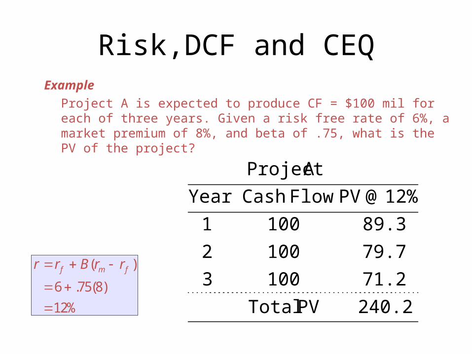
Risk,DCF and CEQExample
Project A is expected to produce CF = $100 mil for each of three years. Given a risk free rate of 6%, a market premium of 8%, and beta of .75, what is the PV of the project?
%12
)8(75.6
)(
fmf rrBrr
240.2 PVTotal
71.21003
79.71002
89.31001
12% @ PV FlowCashYear
AProject

Risk,DCF and CEQExample
Project A is expected to produce CF = $100 mil for each of three years. Given a risk free rate of 6%, a market premium of 8%, and beta of .75, what is the PV of the project?
%12
)8(75.6
)(
fmf rrBrr
240.2 PVTotal
71.21003
79.71002
89.31001
12% @ PV FlowCashYear
AProject
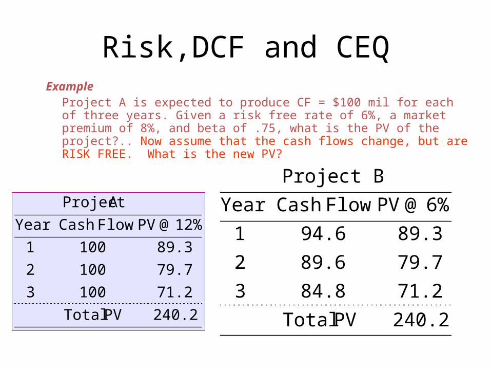
Now assume that the cash flows change, but are RISK FREE. What is the new PV?
Risk,DCF and CEQExample
Project A is expected to produce CF = $100 mil for each of three years. Given a risk free rate of 6%, a market premium of 8%, and beta of .75, what is the PV of the project?.. Now assume that the cash flows change, but are RISK FREE. What is the new PV?
240.2 PVTotal
71.284.83
79.789.62
89.394.61
6% @ PV FlowCashYear
Project B
240.2 PVTotal
71.21003
79.71002
89.31001
12% @ PV FlowCashYear
AProject
Since the 94.6 is risk free, we call it a Certainty Equivalent of the 100.
Risk,DCF and CEQExample
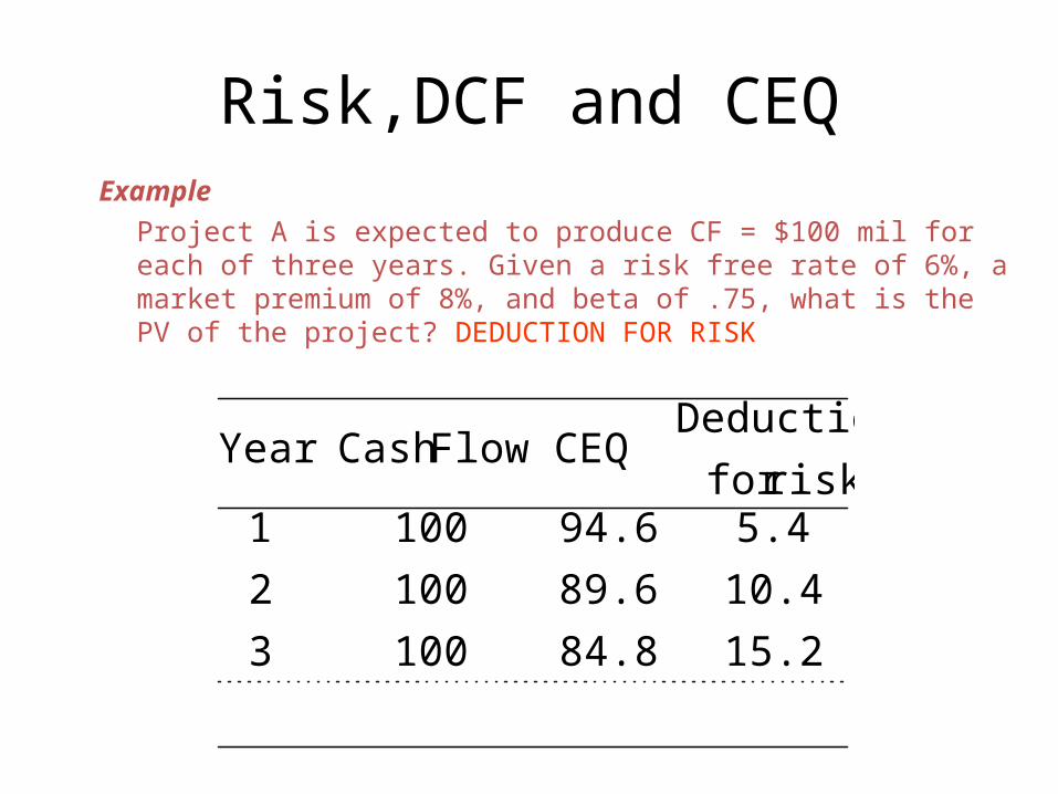
Project A is expected to produce CF = $100 mil for each of three years. Given a risk free rate of 6%, a market premium of 8%, and beta of .75, what is the PV of the project? DEDUCTION FOR RISK
15.284.81003
10.489.61002
5.494.61001riskfor
DeductionCEQFlowCash Year
Risk,DCF and CEQExample
Project A is expected to produce CF = $100 mil for each of three years. Given a risk free rate of 6%, a market premium of 8%, and beta of .75, what is the PV of the project?.. Now assume that the cash flows change, but are RISK FREE. What is the new PV?
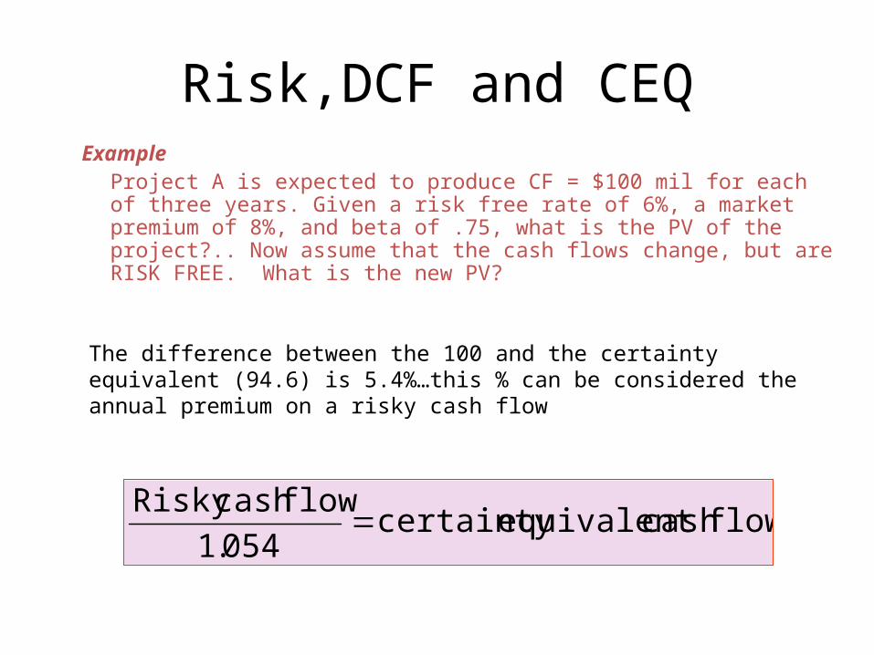
The difference between the 100 and the certainty equivalent (94.6) is 5.4%…this % can be considered the annual premium on a risky cash flow
flow cash equivalentcertainty 054.1
flow cashRisky

Risk,DCF and CEQExample
Project A is expected to produce CF = $100 mil for each of three years. Given a risk free rate of 6%, a market premium of 8%, and beta of .75, what is the PV of the project?.. Now assume that the cash flows change, but are RISK FREE. What is the new PV?
8.84054.1
100 3Year
6.89054.1
100 2Year
6.94054.1
100 1Year
3
2