last time normal distribution –density curve (mound shaped) –family indexed by mean and s. d....
TRANSCRIPT
Last Time
• Normal Distribution– Density Curve (Mound Shaped)– Family Indexed by mean and s. d.– Fit to data, using sample mean and s.d.
• Computation of Normal Probabilities– Using Excel function, NORMDIST– And Big Rules of Probability

Reading In Textbook
Approximate Reading for Today’s Material:
Pages 61-62, 66-70, 59-61, 322-326
Approximate Reading for Next Class:
Pages 337-344, 488-498

Normal Density Fitting
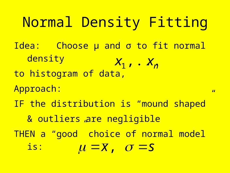
Idea: Choose μ and σ to fit normal density
to histogram of data,
Approach:
IF the distribution is “mound shaped”
& outliers are negligible
THEN a “good” choice of normal model is:
nxx ,...,1
sx ,

Normal Density FittingMelbourne Average Temperature Data
Computation of Normal Probs
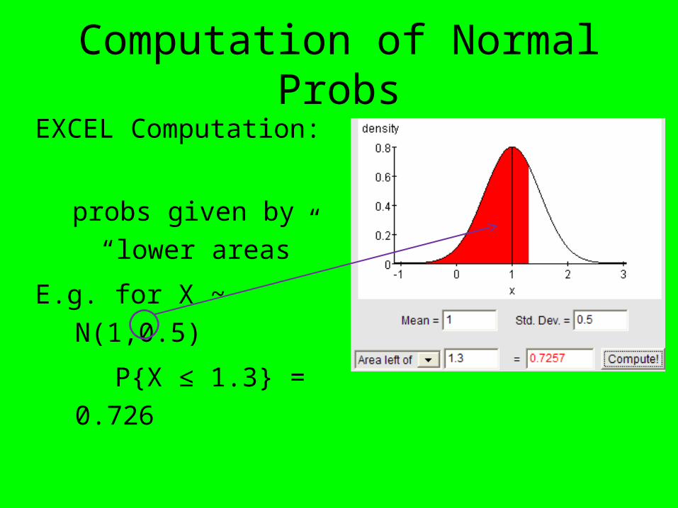
EXCEL Computation:
probs given by “lower
areas”
E.g. for X ~ N(1,0.5)
P{X ≤ 1.3} = 0.726

Computation of Normal Probs
Computation of upper areas:
(use “1 –”, i.e. “not” formula)
= 1 -

Computation of Normal Probs
Computation of areas over intervals:
(use subtraction)
= -

Z-score view of populations
Idea: Reproducible view of “where data point lies in population”

Z-score view of populations
Idea: Reproducible view of “where data point lies in population”
Context 1: List of Numbers
Context 2: Probability distribution

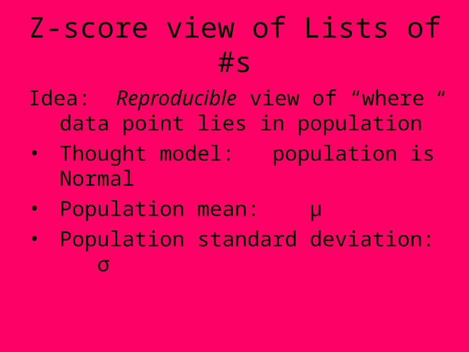
Z-score view of Lists of #s
Idea: Reproducible view of “where data point lies in population”
Z-score view of Lists of #s
Idea: Reproducible view of “where data point lies in population”
• Thought model: population is Normal
Z-score view of Lists of #s
Idea: Reproducible view of “where data point lies in population”
• Thought model: population is Normal
• Population mean: μ
Z-score view of Lists of #s
Idea: Reproducible view of “where data point lies in population”
• Thought model: population is Normal
• Population mean: μ
• Population standard deviation: σ

Z-score view of Lists of #s
Idea: Reproducible view of “where data point lies in population”
• Thought model: population is Normal
• Population mean: μ
• Population standard deviation: σ
Interpret data as “s.d.s away from mean”

Z-score view of Lists of #s
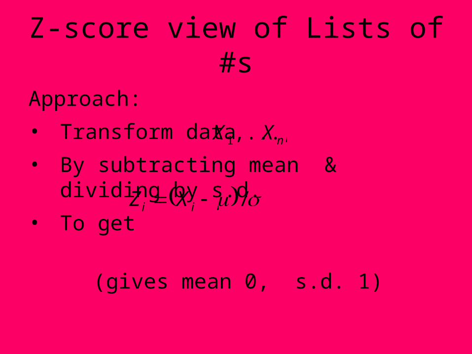
Approach:
• Transform data nXX ,...,1

Z-score view of Lists of #s
Approach:
• Transform data
• By subtracting mean & dividing by s.dnXX ,...,1

Z-score view of Lists of #s
Approach:
• Transform data
• By subtracting mean & dividing by s.d.
• To get
nXX ,...,1
/ ii XZ
Z-score view of Lists of #s
Approach:
• Transform data
• By subtracting mean & dividing by s.d.
• To get
(gives mean 0, s.d. 1)
nXX ,...,1
/ ii XZ

Z-score view of Lists of #s
Approach:
• Transform data
• By subtracting mean & dividing by s.d.
• To get
(gives mean 0, s.d. 1)
• Interpret as
nXX ,...,1
/ ii XZ
ii ZX

Z-score view of Lists of #s
Approach:
• Transform data
• By subtracting mean & dividing by s.d.
• To get
(gives mean 0, s.d. 1)
• Interpret as
• I.e. “ is sd’s above the mean”
nXX ,...,1
/ ii XZ
ii ZX
iX iZ

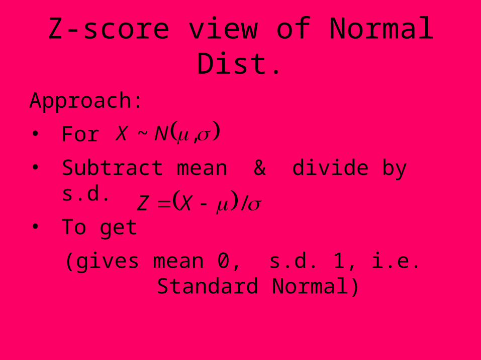
Z-score view of Normal Dist.
Approach:
• For ,~ NX

Z-score view of Normal Dist.
Approach:
• For
• Subtract mean & divide by s.d
,~ NX

Z-score view of Normal Dist.
Approach:
• For
• Subtract mean & divide by s.d.
• To get
,~ NX
/ XZ
Z-score view of Normal Dist.
Approach:
• For
• Subtract mean & divide by s.d.
• To get
(gives mean 0, s.d. 1, i.e. Standard Normal)
,~ NX
/ XZ

Z-score view of Normal Dist.
Approach:
• For
• Subtract mean & divide by s.d.
• To get
(gives mean 0, s.d. 1, i.e. Standard Normal)
• Interpret as
,~ NX
/ XZ
ZX

Z-score view of Normal Dist.
Approach:
• For
• Subtract mean & divide by s.d.
• To get
(gives mean 0, s.d. 1, i.e. Standard Normal)
• Interpret as
• I.e. “ is sd’s above the mean”
,~ NX
/ XZ
ZXX Z

Z-score view of Normal Dist.
HW:
1.117
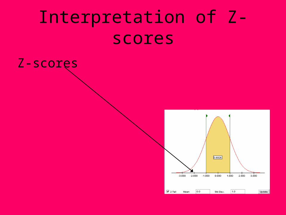
Interpretation of Z-scores
Z-scores

Interpretation of Z-scores
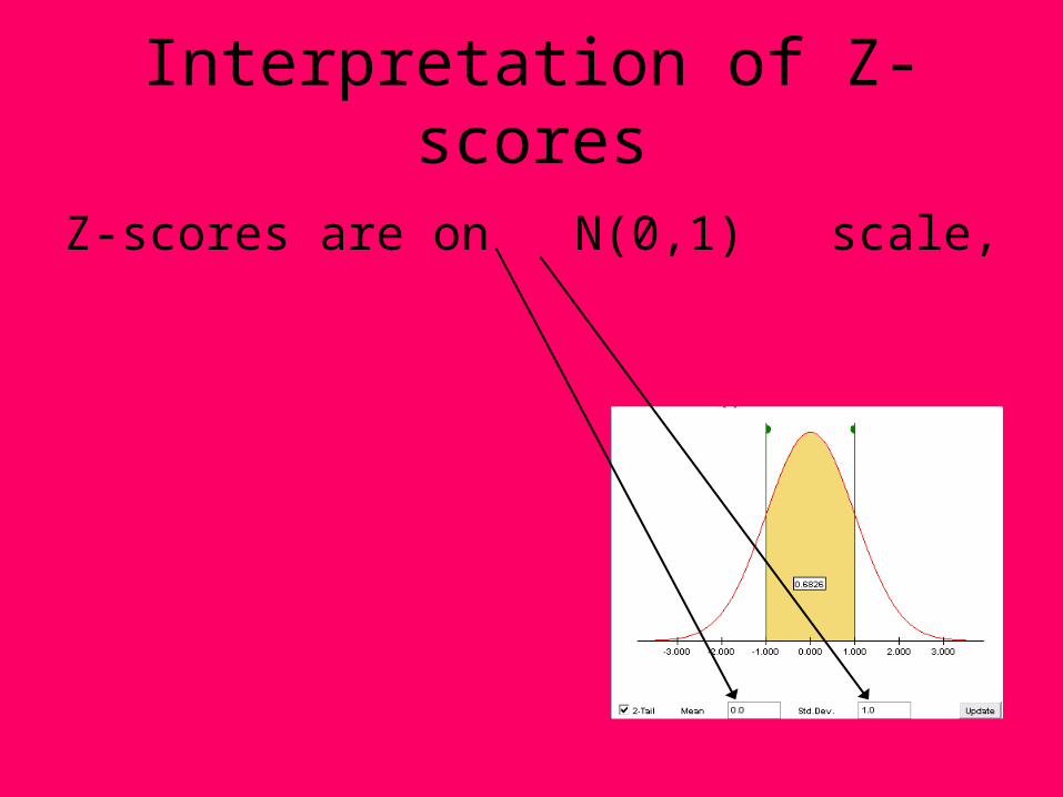
Z-scores are on N(0,1) scale,
Interpretation of Z-scores
Z-scores are on N(0,1) scale,

Interpretation of Z-scores
Z-scores are on N(0,1) scale,
so use areas to interpret them

Interpretation of Z-scores
Z-scores are on N(0,1) scale,
so use areas to interpret them
Important Areas:

Interpretation of Z-scores
Z-scores are on N(0,1) scale,
so use areas to interpret them
Important Areas:
1. Within 1 sd of mean

Interpretation of Z-scores
Z-scores are on N(0,1) scale,
so use areas to interpret them
Important Areas:
1. Within 1 sd of mean

Interpretation of Z-scores
Z-scores are on N(0,1) scale,
so use areas to interpret them
Important Areas:
1. Within 1 sd of mean
“the majority”

Interpretation of Z-scores
Z-scores are on N(0,1) scale,
so use areas to interpret them
Important Areas:
1. Within 1 sd of mean
“the majority”
≈ 68%
Interpretation of Z-scores
Z-scores are on N(0,1) scale,
so use areas to interpret them
Important Areas:
2. Within 2 sd of mean
“really most”
≈ 95%
Interpretation of Z-scores
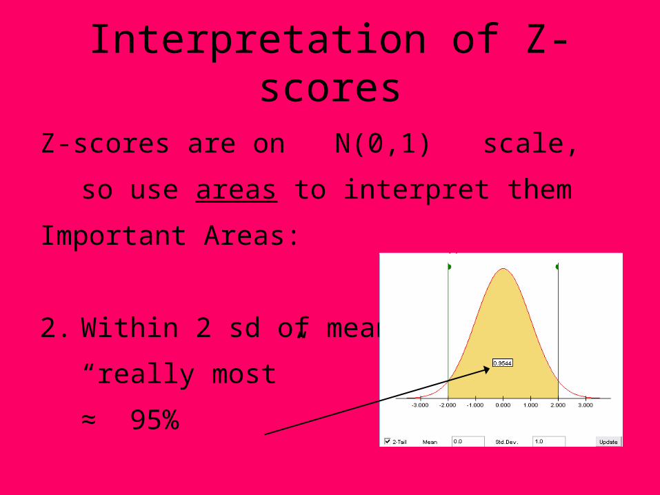
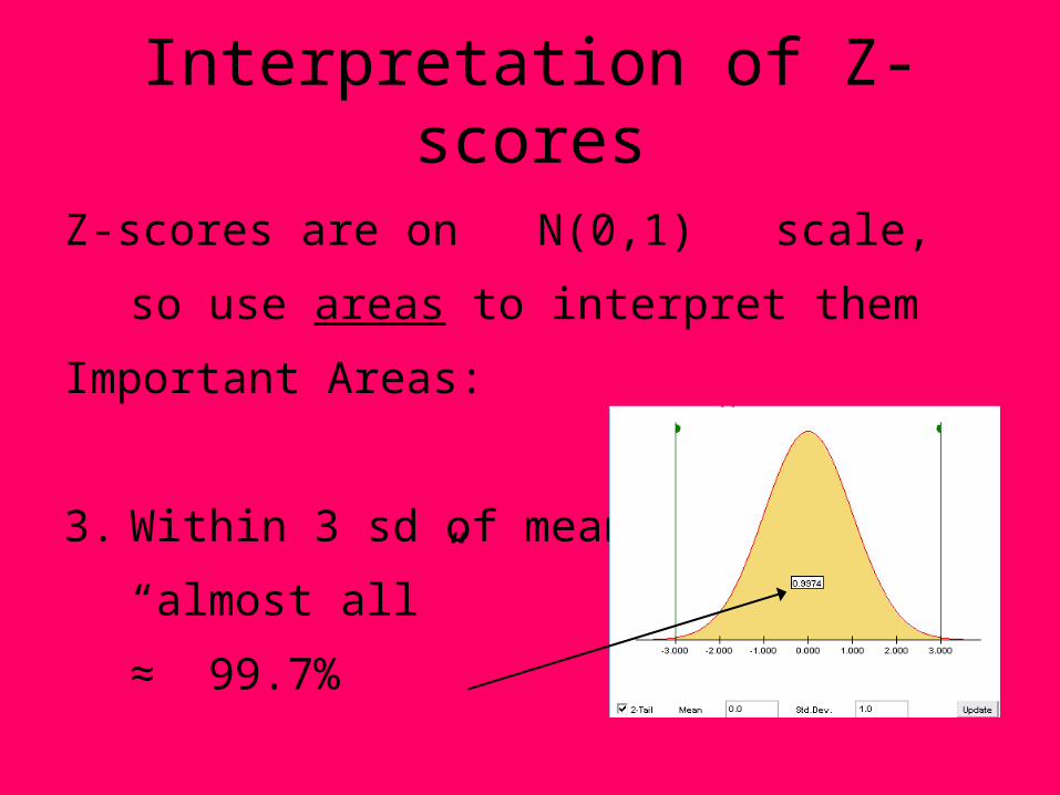
Z-scores are on N(0,1) scale,
so use areas to interpret them
Important Areas:
3. Within 3 sd of mean
“almost all”
≈ 99.7%

Interpretation of Z-scores
Summary: these are called the
“68 - 95 - 99.7 % Rule”

Interpretation of Z-scores
Summary: these are called the
“68 - 95 - 99.7 % Rule”
Mean +- 1 - 2 – 3 sd’s

Interpretation of Z-scores
Summary: “68 - 95 - 99.7 % Rule”
Excel Calculation
From Class Example 9:http://www.stat-or.unc.edu/webspace/courses/marron/UNCstor155-2009/ClassNotes/Stor155Eg9.xls

Interpretation of Z-scores
Summary: “68 - 95 - 99.7 % Rule”
Excel Calculation

Interpretation of Z-scores
HW:
1.115, 1.116 (50%, 2.5%, 0.18-0.22)
1.119

Inverse Normal Probs
Idea, for a given cutoff value, x

Inverse Normal Probs
Idea, for a given cutoff value, x
Calculated
P{X < x}

Inverse Normal Probs
Idea, for a given cutoff value, x
Calculated
P{X < x}
as Area under
normal density

Inverse Normal Probs
Idea, for a given cutoff value, x
Calculated
P{X < x}
as Area under
normal density
Using Excel function:
NORMDIST

Inverse Normal Probs
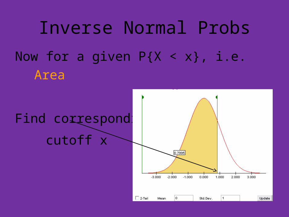
Now for a given P{X < x}, i.e. Area
Inverse Normal Probs
Now for a given P{X < x}, i.e. Area
Find corresponding
cutoff x

Inverse Normal Probs
Now for a given P{X < x}, i.e. Area
Find corresponding
cutoff x
Terminology:

Inverse Normal Probs
Now for a given P{X < x}, i.e. Area
Find corresponding
cutoff x
Terminology:
• Quantile

Inverse Normal Probs
Now for a given P{X < x}, i.e. Area
Find corresponding
cutoff x
Terminology:
• Quantile
• Percentile

Inverse Normal Probs
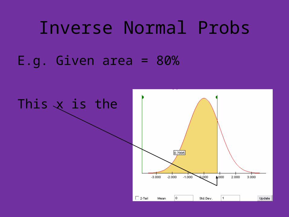
E.g. Given area = 80%
Inverse Normal Probs
E.g. Given area = 80%
This x is the

Inverse Normal Probs
E.g. Given area = 80%
This x is the
• 0.8-quantile

Inverse Normal Probs
E.g. Given area = 80%
This x is the
• 0.8-quantile
• 80-th percentile

Inverse Normal Probs
Now for a given P{X < x}, i.e. Area
Find:
• Quantile
• Percentile

Inverse Normal Probs
Now for a given P{X < x}, i.e. Area
Find:
• Quantile
• Percentile
Excel Computation:
NORMINV

Inverse Normal Probs
Excel Computation:
NORMINV

Inverse Normal Probs
Excel Computation:
NORMINV
(very similar to other Excel functions)

Inverse Normal Probs
Excel Computation:
NORMINV
(very similar to other Excel functions)
(and reasonably well organized)
Inverse Normal Probs
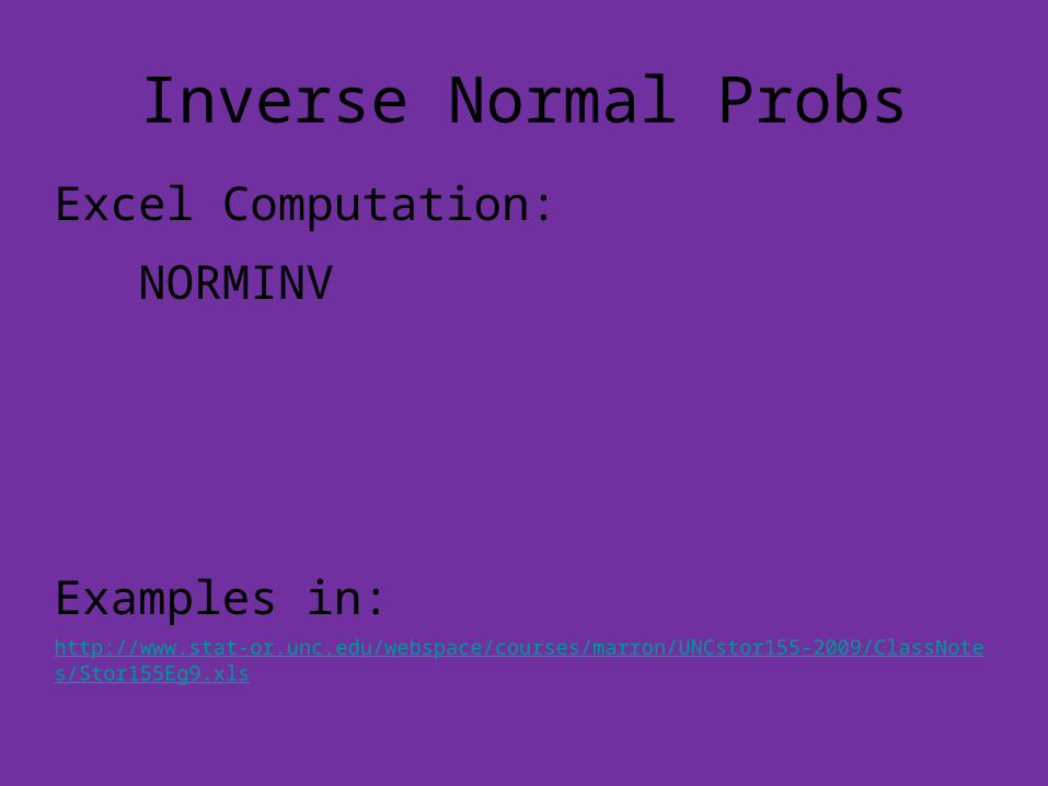
Excel Computation:
NORMINV
Examples in:http://www.stat-or.unc.edu/webspace/courses/marron/UNCstor155-2009/ClassNotes/Stor155Eg9.xls

Inverse Normal Probs
Excel Computation:
NORMINV

Inverse Normal Probs
Excel Computation:
NORMINV
Set:
Mean = 0

Inverse Normal Probs
Excel Computation:
NORMINV
Set:
Mean = 0
s.d. = 1
prob = 0.8

Inverse Normal Probs
Excel Computation:
NORMINV
Set:
Mean = 0
s.d. = 1
prob = 0.8
Get answer

Inverse Normal Probs
Excel Computation:
NORMINV
or can just
type in
formula

Inverse Normal Probs
Excel Computation:
NORMINV
or can just
type in
formula
Get answer

Inverse Normal Probs
Now for a given P{X < x}, i.e. Area
Find:
• Quantile
• Percentile
= 0.84
Inverse Normal Probs
Excel Computation: NORMINV
Another example: for X ~ N(100,20)

Inverse Normal Probs
Excel Computation: NORMINV
Another example: for X ~ N(100,20)

Inverse Normal Probs
Excel Computation: NORMINV
Another example: for X ~ N(100,20)
Find x, so that 30% = P{X < x}

Inverse Normal Probs
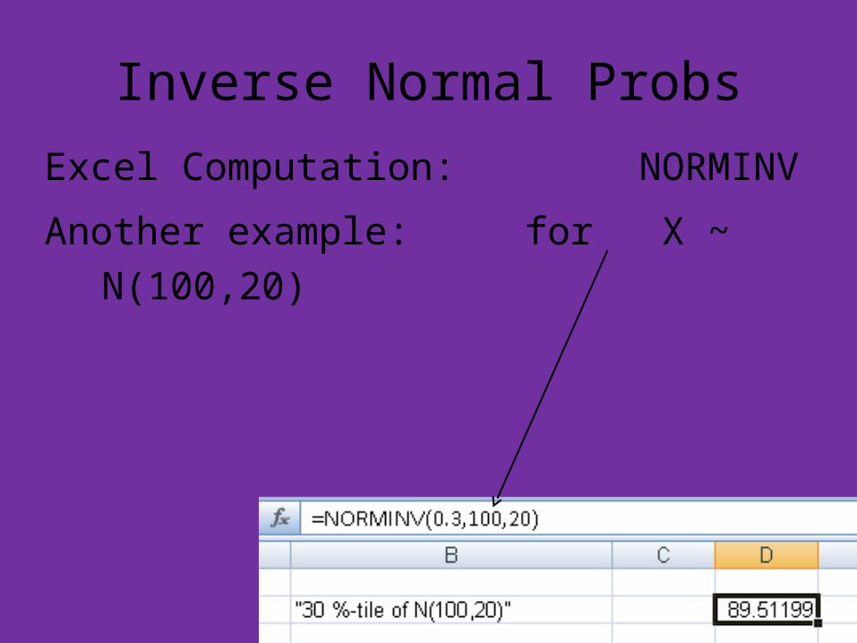
Excel Computation: NORMINV
Another example: for X ~ N(100,20)
Find x, so that 30% = P{X < x}
i.e. the 30-th percentile

Inverse Normal Probs
Excel Computation: NORMINV
Another example: for X ~ N(100,20)
Find x, so that 30% = P{X < x}
i.e. the 30-th percentile
Answer:
slightly less
than mean

Inverse Normal Probs
Example: Quality Control

Inverse Normal Probs
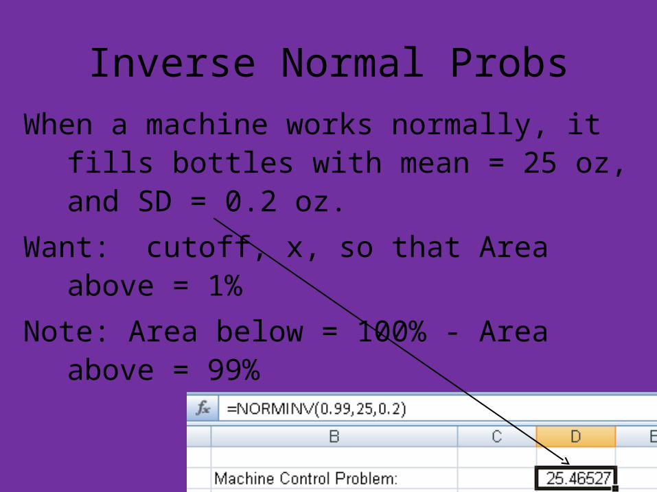
When a machine works normally, it fills bottles with mean = 25 oz, and SD = 0.2 oz.

Inverse Normal Probs
When a machine works normally, it fills bottles with mean = 25 oz, and SD = 0.2 oz.
The machine is “out of control” when it overfills.

Inverse Normal Probs
When a machine works normally, it fills bottles with mean = 25 oz, and SD = 0.2 oz.
The machine is “out of control” when it overfills. Choose an “alarm level”, which will give only 1 % false alarms.

Inverse Normal Probs
When a machine works normally, it fills bottles with mean = 25 oz, and SD = 0.2 oz.
The machine is “out of control” when it overfills. Choose an “alarm level”, which will give only 1 % false alarms.
Want: cutoff, x, so that Area above = 1%

Inverse Normal Probs
When a machine works normally, it fills bottles with mean = 25 oz, and SD = 0.2 oz.
The machine is “out of control” when it overfills. Choose an “alarm level”, which will give only 1 % false alarms.
Want: cutoff, x, so that Area above = 1%
Note: Area below = 100% - Area above = 99%

Inverse Normal Probs
When a machine works normally, it fills bottles with mean = 25 oz, and SD = 0.2 oz.
Want: cutoff, x, so that Area above = 1%
Note: Area below = 100% - Area above = 99%

Inverse Normal Probs
When a machine works normally, it fills bottles with mean = 25 oz, and SD = 0.2 oz.
Want: cutoff, x, so that Area above = 1%
Note: Area below = 100% - Area above = 99%

Inverse Normal Probs
When a machine works normally, it fills bottles with mean = 25 oz, and SD = 0.2 oz.
Want: cutoff, x, so that Area above = 1%
Note: Area below = 100% - Area above = 99%

Inverse Normal Probs
When a machine works normally, it fills bottles with mean = 25 oz, and SD = 0.2 oz.
Want: cutoff, x, so that Area above = 1%
Note: Area below = 100% - Area above = 99%
Inverse Normal Probs
When a machine works normally, it fills bottles with mean = 25 oz, and SD = 0.2 oz.
Want: cutoff, x, so that Area above = 1%
Note: Area below = 100% - Area above = 99%

Inverse Normal Probs
When a machine works normally, it fills bottles with mean = 25 oz, and SD = 0.2 oz.
Want: cutoff, x, so that Area above = 1%
Note: Area below = 100% - Area above = 99%
So set alarm threshold to 25.47

Inverse Normal Probs
HW:
1.122 (-0.675, 0.385)
1.123
1.132 (1294)
1.133
1.139

And Now for Something Completely Different
A fun idea. Can you read this?

And Now for Something Completely Different
A fun idea. Can you read this?
Olny srmat poelpe can raed this.

And Now for Something Completely Different
A fun idea. Can you read this?
Olny srmat poelpe can raed this.
I cdnuolt blveiee that I cluod aulaclty uesdnatnrd what I was rdanieg.

And Now for Something Completely Different
A fun idea. Can you read this?
Olny srmat poelpe can raed this.
I cdnuolt blveiee that I cluod aulaclty uesdnatnrd what I was rdanieg.
The phaonmneal pweor of the hmuan mnid, aoccdrnig to rscheearch at Cmabrigde Uinervtisy.

And Now for Something Completely Different
The phaonmneal pweor of the hmuan mnid, aoccdrnig to rscheearch at Cmabrigde Uinervtisy.

And Now for Something Completely Different
The phaonmneal pweor of the hmuan mnid, aoccdrnig to rscheearch at Cmabrigde Uinervtisy.
It deosn't mttaer in what oredr the ltteers in a word are, the olny iprmoatnt tihng is that the first and last ltteer be in the rghit pclae.

And Now for Something Completely Different
The phaonmneal pweor of the hmuan mnid, aoccdrnig to rscheearch at Cmabrigde Uinervtisy.
It deosn't mttaer in what oredr the ltteers in a word are, the olny iprmoatnt tihng is that the first and last ltteer be in the rghit pclae.
The rset can be a taotl mses and you can still raed it wouthit a porbelm.

And Now for Something Completely Different
The rset can be a taotl mses and you can still raed it wouthit a porbelm.
And Now for Something Completely Different
The rset can be a taotl mses and you can still raed it wouthit a porbelm.
Tihs is bcuseae the huamn mnid deos not raed ervey lteter by istlef, but the word as a wlohe.

And Now for Something Completely Different
The rset can be a taotl mses and you can still raed it wouthit a porbelm.
Tihs is bcuseae the huamn mnid deos not raed ervey lteter by istlef, but the word as a wlohe.
Amzanig huh?

And Now for Something Completely Different
The rset can be a taotl mses and you can still raed it wouthit a porbelm.
Tihs is bcuseae the huamn mnid deos not raed ervey lteter by istlef, but the word as a wlohe.
Amzanig huh?
Yaeh and I awlyas tghuhot slpeling was ipmorantt!

Checking Normality
Idea: For which data sets, will the normal
distribution be a good model?

Checking Normality
Idea: For which data sets, will the normal
distribution be a good model?
Recall fitting normal density to data:
Normal Density Fitting
Idea: Choose μ and σ to fit normal density
to histogram of data,
Approach:
IF the distribution is “mound shaped”
& outliers are negligible
THEN a “good” choice of normal model is:
nxx ,...,1
sx ,

Normal Density FittingMelbourne Average Temperature Data

Checking Normality
Idea: For which data sets, will the normal
distribution be a good model?
Useful graphical device to check:
IF the distribution is “mound shaped”
& outliers are negligible

Checking Normality
Useful graphical device:

Checking Normality
Useful graphical device:
Quantile – Quantile plot

Checking Normality
Useful graphical device:
Quantile – Quantile plot
Varying Terminology:
Checking Normality
Useful graphical device:
Quantile – Quantile plot
Varying Terminology:
• Q-Q plot

Checking Normality
Useful graphical device:
Quantile – Quantile plot
Varying Terminology:
• Q-Q plot
• Normal Quantile plot (text book)

Checking Normality
Q-Q plot

Checking Normality
Q-Q plot
Idea: graphical comparison
Checking Normality
Q-Q plot
Idea: graphical comparison of
data distribution

Checking Normality
Q-Q plot
Idea: graphical comparison of
data distribution vs. normal distribution

Checking Normality
Q-Q plot
Idea: graphical comparison of
data distribution vs. normal distribution
as
data quantiles vs. normal quantiles

Checking Normality
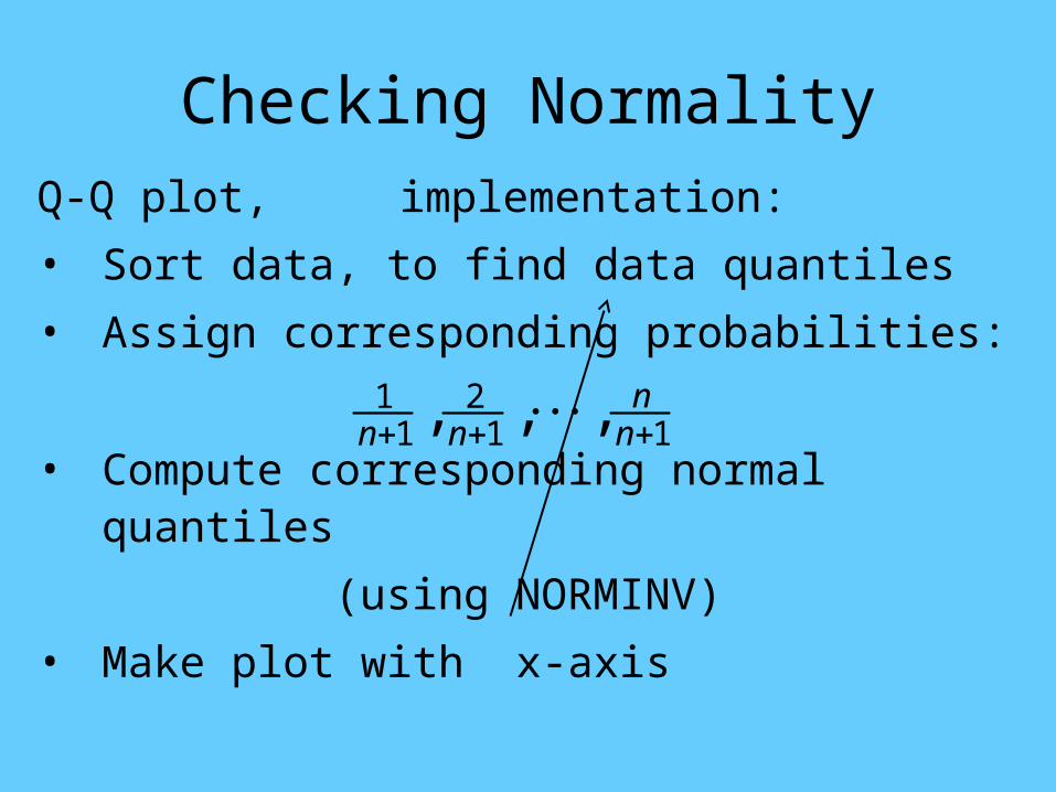
Q-Q plot, implementation:

Checking Normality
Q-Q plot, implementation:
• Sort data, to find data quantiles

Checking Normality
Q-Q plot, implementation:
• Sort data, to find data quantiles
• Assign corresponding probabilities:
112
11 ,,, n
nnn

Checking Normality
Q-Q plot, implementation:
• Sort data, to find data quantiles
• Assign corresponding probabilities:
(equally spaced, strictly between 0 and 1)
112
11 ,,, n
nnn

Checking Normality
Q-Q plot, implementation:
• Sort data, to find data quantiles
• Assign corresponding probabilities:
• Compute corresponding normal quantiles
112
11 ,,, n
nnn

Checking Normality
Q-Q plot, implementation:
• Sort data, to find data quantiles
• Assign corresponding probabilities:
• Compute corresponding normal quantiles
(using NORMINV)
112
11 ,,, n
nnn
Checking Normality
Q-Q plot, implementation:
• Sort data, to find data quantiles
• Assign corresponding probabilities:
• Compute corresponding normal quantiles
(using NORMINV)
• Make plot with x-axis
112
11 ,,, n
nnn

Checking Normality
Q-Q plot, implementation:
• Sort data, to find data quantiles
• Assign corresponding probabilities:
• Compute corresponding normal quantiles
(using NORMINV)
• Make plot with x-axis & y-axis
112
11 ,,, n
nnn

Checking Normality
Q-Q plot, interpretation:

Checking Normality
Q-Q plot, interpretation:
• When distribution is normal:
Checking Normality
Q-Q plot, interpretation:
• When distribution is normal:– Points lie close to a line
Checking Normality
Q-Q plot, interpretation:
• When distribution is normal:– Points lie close to a line
– For standard normal quantiles

Checking Normality
Q-Q plot, interpretation:
• When distribution is normal:– Points lie close to a line
– For standard normal quantiles• Y-intercept of line is mean
• Slope of line is s.d.

Checking Normality
Q-Q plot, interpretation:
• When distribution is normal:– Points lie close to a line
– For standard normal quantiles• Y-intercept of line is mean
• Slope of line is s.d.
• For non-normal distribution:

Checking Normality
Q-Q plot, interpretation:
• When distribution is normal:– Points lie close to a line
– For standard normal quantiles• Y-intercept of line is mean
• Slope of line is s.d.
• For non-normal distribution:– Q-Q plot will curve away from line

Checking Normality
Q-Q plot, e.g.

Checking Normality
Q-Q plot, e.g.
Excel analyses available in:http://www.stat-or.unc.edu/webspace/courses/marron/UNCstor155-2009/ClassNotes/Stor155Eg10.xls

Checking Normality
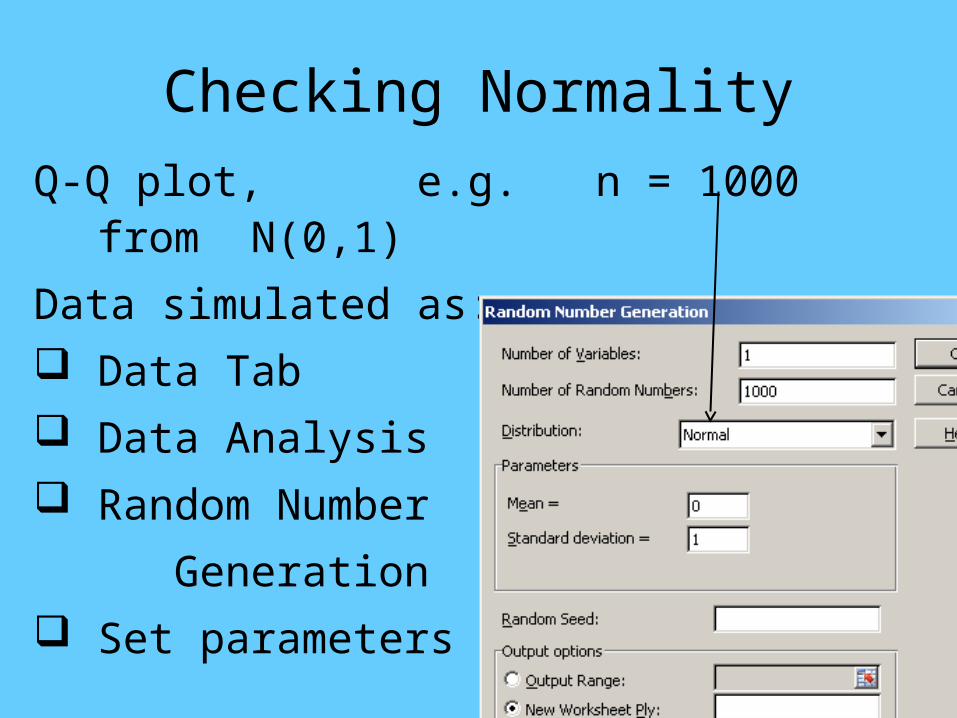
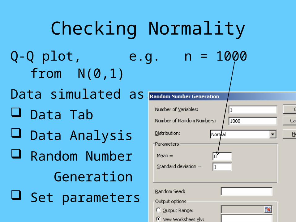
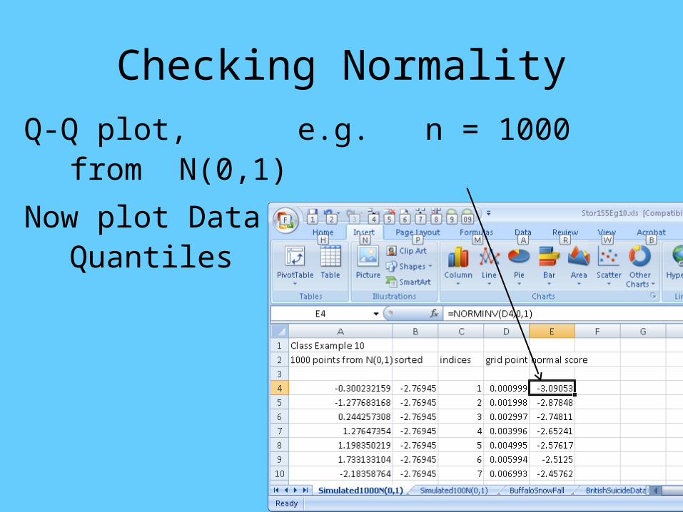
Q-Q plot, e.g. n = 1000 from N(0,1)
Data simulated as:

Checking Normality
Q-Q plot, e.g. n = 1000 from N(0,1)
Data simulated as:
Data Tab

Checking Normality
Q-Q plot, e.g. n = 1000 from N(0,1)
Data simulated as:
Data Tab
Data Analysis

Checking Normality
Q-Q plot, e.g. n = 1000 from N(0,1)
Data simulated as:
Data Tab
Data Analysis
Random Number
Generation

Checking Normality
Q-Q plot, e.g. n = 1000 from N(0,1)
Data simulated as:
Data Tab
Data Analysis
Random Number
Generation
Set parameters
Checking Normality
Q-Q plot, e.g. n = 1000 from N(0,1)
Data simulated as:
Data Tab
Data Analysis
Random Number
Generation
Set parameters
Checking Normality
Q-Q plot, e.g. n = 1000 from N(0,1)
Data simulated as:
Data Tab
Data Analysis
Random Number
Generation
Set parameters

Checking Normality
Q-Q plot, e.g. n = 1000 from N(0,1)
Data simulated as:
Data Tab
Data Analysis
Random Number
Generation
Set parameters

Checking Normality
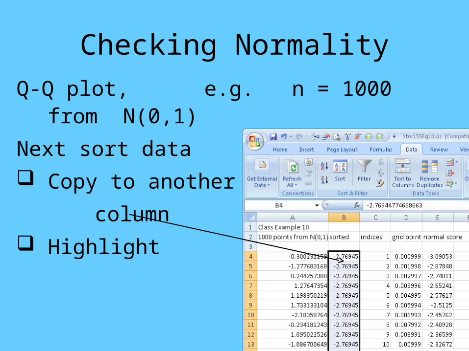
Q-Q plot, e.g. n = 1000 from N(0,1)
Next sort data
Copy to another
column
Checking Normality
Q-Q plot, e.g. n = 1000 from N(0,1)
Next sort data
Copy to another
column
Highlight

Checking Normality
Q-Q plot, e.g. n = 1000 from N(0,1)
Next sort data
Copy to another
column
Highlight
Data Tab

Checking Normality
Q-Q plot, e.g. n = 1000 from N(0,1)
Next sort data
Copy to another
column
Highlight
Data Tab
Sort Button

Checking Normality
Q-Q plot, e.g. n = 1000 from N(0,1)
Next sort data
Copy to another
column
Highlight
Data Tab
Sort Button
Gives Data Quantiles

Checking Normality
Q-Q plot, e.g. n = 1000 from N(0,1)
Next compute Normal Quantiles
Checking Normality
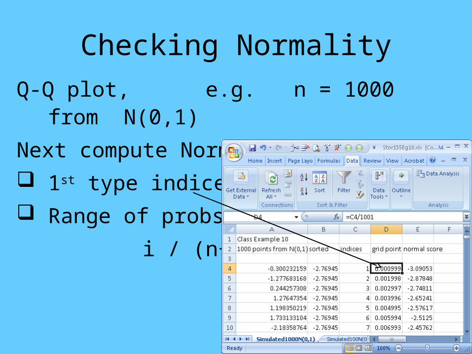
Q-Q plot, e.g. n = 1000 from N(0,1)
Next compute Normal Quantiles
1st type indices
Range of probs
i / (n+1)
Checking Normality
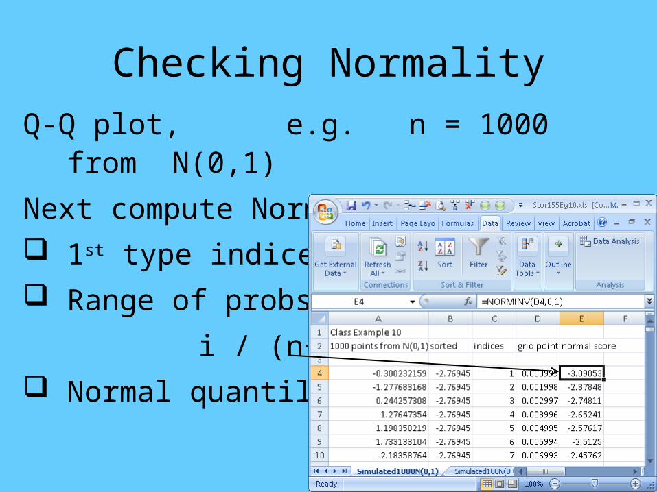
Q-Q plot, e.g. n = 1000 from N(0,1)
Next compute Normal Quantiles
1st type indices
Range of probs
i / (n+1)
Normal quantiles

Checking Normality
Q-Q plot, e.g. n = 1000 from N(0,1)
Now plot Data Quantiles vs. Normal Quantiles
Checking Normality
Q-Q plot, e.g. n = 1000 from N(0,1)
Now plot Data Quantiles vs. Normal Quantiles

Checking Normality
Q-Q plot, e.g. n = 1000 from N(0,1)
Now plot Data Quantiles vs. Normal Quantiles
Insert Tab

Checking Normality
Q-Q plot, e.g. n = 1000 from N(0,1)
Now plot Data Quantiles vs. Normal Quantiles
Insert Tab
Scatter
Button

Checking Normality
Q-Q plot, e.g. n = 1000 from N(0,1)
Now plot Data Quantiles vs. Normal Quantiles
Insert Tab
Scatter
Button
Fill out menu
(as before)

Checking Normality
Q-Q plot, e.g. n = 1000 from N(0,1)
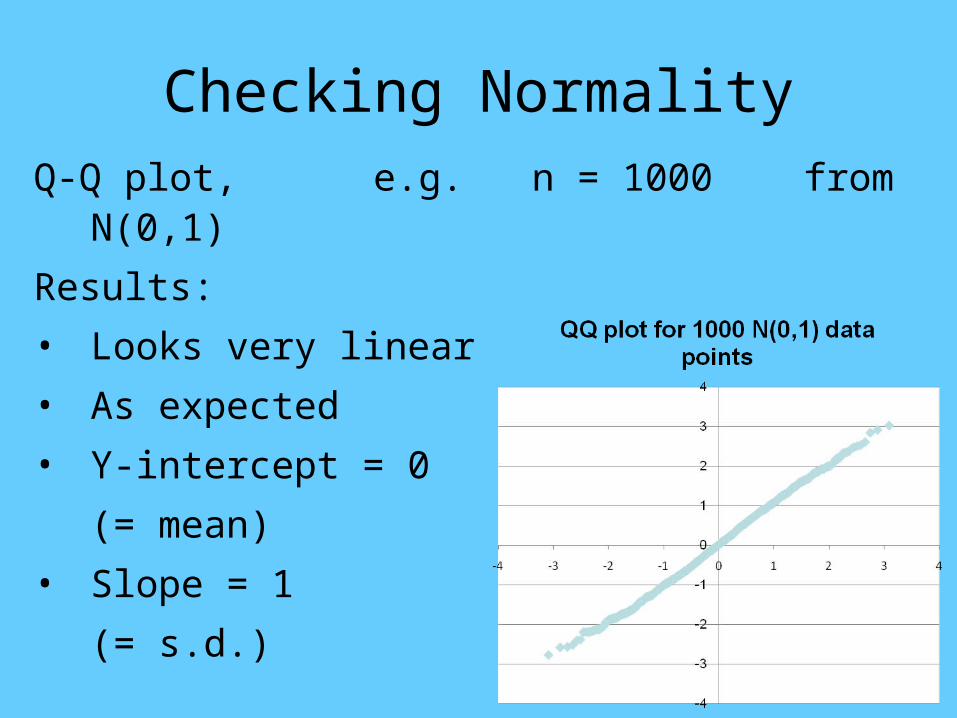
Results:
• Looks very linear

Checking Normality
Q-Q plot, e.g. n = 1000 from N(0,1)
Results:
• Looks very linear
• As expected

Checking Normality
Q-Q plot, e.g. n = 1000 from N(0,1)
Results:
• Looks very linear
• As expected
• Y-intercept = 0
(= mean)
Checking Normality
Q-Q plot, e.g. n = 1000 from N(0,1)
Results:
• Looks very linear
• As expected
• Y-intercept = 0
(= mean)
• Slope = 1
(= s.d.)

Checking Normality
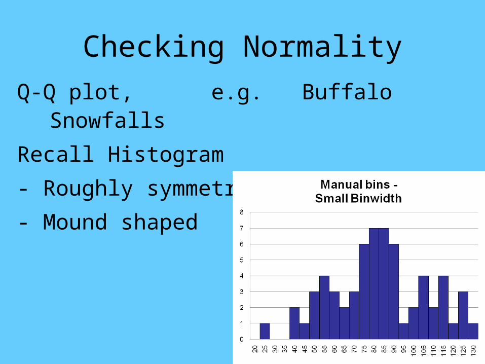
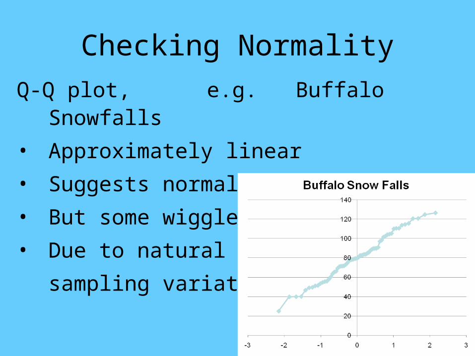
Q-Q plot, e.g. Buffalo Snowfalls

Checking Normality
Q-Q plot, e.g. Buffalo Snowfalls
Recall Histogram

Checking Normality
Q-Q plot, e.g. Buffalo Snowfalls
Recall Histogram
- Roughly symmetric
Checking Normality
Q-Q plot, e.g. Buffalo Snowfalls
Recall Histogram
- Roughly symmetric
- Mound shaped

Checking Normality
Q-Q plot, e.g. Buffalo Snowfalls
Recall Histogram
- Roughly symmetric
- Mound shaped
- Does Normal Curve
fit the data?

Checking Normality
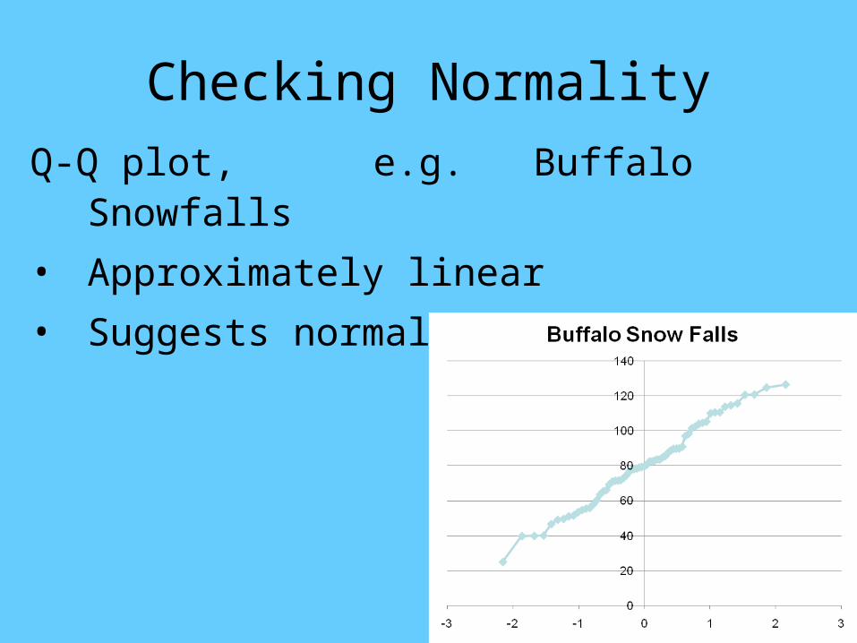
Q-Q plot, e.g. Buffalo Snowfalls
• Approximately linear
Checking Normality
Q-Q plot, e.g. Buffalo Snowfalls
• Approximately linear
• Suggests normal

Checking Normality
Q-Q plot, e.g. Buffalo Snowfalls
• Approximately linear
• Suggests normal
• But some wiggles?
Checking Normality
Q-Q plot, e.g. Buffalo Snowfalls
• Approximately linear
• Suggests normal
• But some wiggles?
• Due to natural
sampling variation?

Checking Normality
Q-Q plot, e.g. Buffalo Snowfalls
• Approximately linear
• Suggests normal
• But some wiggles?
• Due to natural
sampling variation?
Study with smaller
simulation

Checking Normality
Q-Q plot, e.g. n = 100 from N(0,1)

Checking Normality
Q-Q plot, e.g. n = 100 from N(0,1)
• Approximately linear

Checking Normality
Q-Q plot, e.g. n = 100 from N(0,1)
• Approximately linear
• Some wiggliness

Checking Normality
Q-Q plot, e.g. n = 100 from N(0,1)
• Approximately linear
• Some wiggliness
• Suggests Buffalo
variation is usual

Checking Normality
Q-Q plot, e.g. n = 100 from N(0,1)
• Approximately linear
• Some wiggliness
• Suggests Buffalo
variation is usual
• Make this more
precise?
Checking Normality
Q-Q plot, e.g. British Suicides

Checking Normality
Q-Q plot, e.g. British Suicides
Recall Histogram

Checking Normality
Q-Q plot, e.g. British Suicides
Recall Histogram
Strong right skewness

Checking Normality
Q-Q plot, e.g. British Suicides
Recall Histogram
Strong right skewness
So mean >> median

Checking Normality
Q-Q plot, e.g. British Suicides
Recall Histogram
Strong right skewness
So mean >> median
Not mound shaped

Checking Normality
Q-Q plot, e.g. British Suicides

Checking Normality
Q-Q plot, e.g. British Suicides
• Distinct non-linearity (curvature)

Checking Normality
Q-Q plot, e.g. British Suicides
• Distinct non-linearity (curvature)
• Conclude data
not normal

Checking Normality
Q-Q plot, e.g. British Suicides
• Distinct non-linearity (curvature)
• Conclude data
not normal
• Characteristic of
right skewness

Checking Normality
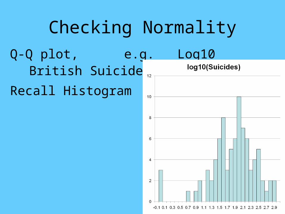
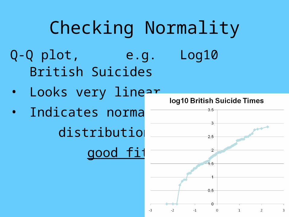
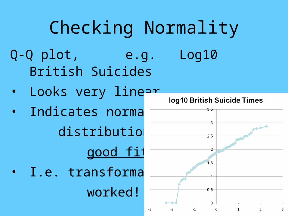
Q-Q plot, e.g. Log10 British Suicides
Recall:
log10 transformation resulted in mound shape
Checking Normality
Q-Q plot, e.g. Log10 British Suicides
Recall Histogram

Checking Normality
Q-Q plot, e.g. Log10 British Suicides
Recall Histogram:
o Much more mound
shaped

Checking Normality
Q-Q plot, e.g. Log10 British Suicides
Recall Histogram:
o Much more mound
shaped
o Check for
normality with
Q-Q plot

Checking Normality
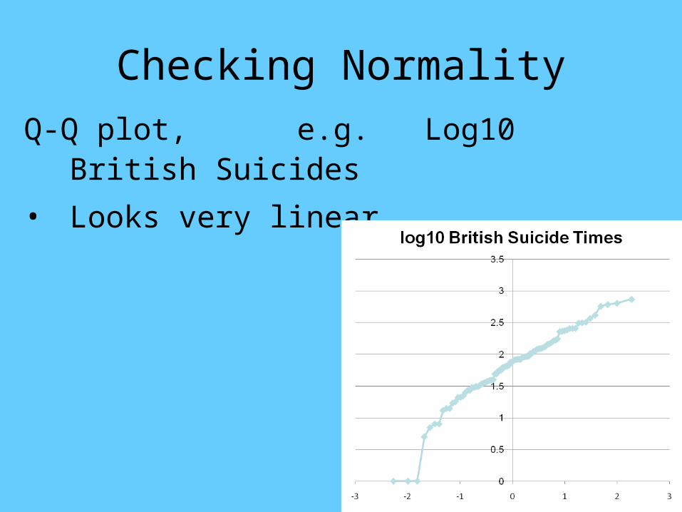
Q-Q plot, e.g. Log10 British Suicides
Checking Normality
Q-Q plot, e.g. Log10 British Suicides
• Looks very linear
Checking Normality
Q-Q plot, e.g. Log10 British Suicides
• Looks very linear
• Indicates normal
distribution is
good fit
Checking Normality
Q-Q plot, e.g. Log10 British Suicides
• Looks very linear
• Indicates normal
distribution is
good fit
• I.e. transformation
worked!

Checking Normality
HW:
1.143
1.145
1.146 (a. approx. normal + big outlier; b. close to normal; c. right skew + one big outlier; d. Non-normal with several clusters