Latent Topics-based Relevance Feedback

for Video Retrieval

Ruben Fernandez-Beltran, Filiberto Pla

Institut of New Imaging Technologies, Universitat Jaume I, SPAIN

Abstract

This work presents a novel Content-Based Video Retrieval approach in

order to cope with the semantic gap challenge by means of latent topics.

Firstly, a supervised topic model is proposed to transform the classical re-

trieval approach into a class discovery problem. Subsequently, a new proba-

bilistic ranking function is deduced from that model to tackle the semantic

gap between low-level features and high-level concepts. Finally, a short-

term relevance feedback scheme is defined where queries can be initialised

with samples from inside or outside the database. Several retrieval simula-

tions have been carried out using three databases and seven different ranking

functions to test the performance of the presented approach. Experiments

revealed that the proposed ranking function is able to provide a competitive

advantage within the content-based retrieval field.

Keywords:

Content-Based Video Retrieval, Relevance Feedback, Latent Topics,

probabilistic Latent Semantic Analysis (pLSA), Information Retrieval

Preprint submitted to Pattern Recognition July 10, 2015

1. Introduction

The low cost of image/video capture technology together with the increas-

ing capacity of storage is producing a huge expansion of video collections. In

this scenario, one of the most important challenges is how to retrieve users’

relevant data from this vast amount of information. Content-Based Video

Retrieval (CBVR) is concerned about providing users with those videos which

satisfy their queries by means of the video content analysis. As a result, the

CBVR field has become a very important research area and a wide variety

of CBVR systems have been developed [1, 2, 3, 4]. The standard CBVR

procedure involves three main components: (i) a query, containing a few

video examples of the semantic concept that the user is looking for; (ii) a

database, which is used to retrieve videos related to the query concept; and

(iii) a ranking function, which sorts the database according to the relevance

with respect to the user’s query. These three components are typically inte-

grated with the user in a Relevance Feedback (RF) scheme [5] to provide the

most relevant videos through several feedback iterations.

Figure 1 shows the general RF scheme for retrieval. At the initialisation

stage (stage 0), the user introduces the query concept into the system by

providing Q examples of the concept of interest. Then, the interactive process

consists of the alternation of two stages through I feedback iterations. In

the retrieval stage (stage 1), the system ranks the database according to

the query and shows the S top items (scope) to the user. In the feedback

stage (stage 2), the user checks the scope to select the correctly retrieved

samples and finally the query is expanded with these new positive examples

to carry out the next iteration. The ranking function can be considered the

2

Figure 1: Relevance Feedback scheme. Q is the number of initial examples in the query,

I the number of feedback iterations and S the number of top ranked samples.

kernel of the retrieval system because it is in charge of scoring the samples of

the database according to the query. As a result, the nature of the ranking

function and the nature of the video representation space where the ranking

function works are two of the most important factors for the precision of a

CBVR system.

1.1. Ranking functions

One of the most common rankings in multimedia retrieval is the distance-

based ranking. Such ranking is performed according to the minimum distance

or maximum similarity in the video representation space. Several functions

have been proposed in the content-based retrieval field. For instance, in [6] an

image retrieval systems is presented which is based on an Euclidean ranking

of micro-structure features that combine color, texture and shape. In other

works, such as [7], the retrieval ranking is performed using combinations of

similarity measures. Even, some authors [8] have combined several descrip-

tors and distance measures to rank the database. Nevertheless, these kinds

3

of functions tend to perform poorer when the query concepts to retrieve are

rather complex [9].

Other ranking algorithms are based on inductive learning [10, 11] which

typically use a bank of classifiers to represent the set of possible events to test.

However, this approach usually leads to a constrained retrieval scheme where

users are not allowed to search whatever they want. The CBVR problem itself

has an unconstrained nature [9, 12] because the concept to retrieve is a priori

unknown. Moreover, the performance of these methods highly depends on

the used training data but in the CBVR application the initialisation and

feedback are often too limited to provide a consistent training set.

Alternative ranking methods are based on transductive ranking. They

use the own topology of the data to improve the output ranking. One of

the most representative ones is Manifold Ranking (MR) [13] which ranks

the data with respect to the intrinsic data distribution. In a more recent

work [14], Yang et al. present a new transductive ranking function called

Local Regression and Global Alignment (LRGA) to learn a robust Laplacian

matrix which is able to slightly improve the performance of MR. The main

drawback of these methods is their high computational cost because they

require demanding matrix operations over the retrieval process. Transduc-

tive ranking functions are usually applied in the original descriptor space,

however other authors have used a different representation space to perform

the ranking. In [15], Zhang et al. present an image retrieval system which

computes the cosine similarity function in a topic space to rank the database.

This work uses positive (checked) and negative (unchecked) samples in the

interactive retrieval process, but managing negative samples adds an extra

4

effort because users have to check false negatives in addition to true positives.

1.2. Video representation space

Ranking functions run in a specific representation space where videos are

encoded in feature vectors according to the information provided by a de-

scriptor. In the literature, different kinds of descriptors have been proposed

using static information - Scale Invariant Feature Transform (SIFT) [16]),

spatio-temporal - Spatial Temporal Interest Points (STIP) [17]) or audio -

Mel Frequency Cepstral Coefficients (MFCC) [18]. The standard procedure

to encode all this low-level information in feature vectors is the visual Bag

of Words (vBoW) [19]. The vBoW quantisation starts by learning a visual

vocabulary made up of the clustering of the local features. Then, each video

is represented in a single histogram of visual words by accumulating the num-

ber of local features into their closest clusters. Authors usually refer to this

quantised space as descriptor space although it is not the direct output of

the descriptor functions. Some recent works have presented more advanced

descriptors which are able to achieve better results for specific applications.

Wang and Schmid [20] presented a video representation based on dense tra-

jectories specially designed for action recognition which outperforms the most

common motion-based descriptors. However, in unconstrained CBVR the

type of concepts to deal with is so wide that simpler and non-specialised

descriptors are commonly used [4].

1.3. Limitations of current approaches and topic models

Several of the aforementioned approaches have shown to be successful

at retrieval tasks when they are used on reduced databases with a small

5

number of concepts [21]. Nonetheless, the so-called semantic gap [22] between

computable low-level features and query concepts is still a challenge for huge

unconstrained video collections. The visual variability of semantic concepts

is so high that often current approaches are not able to capture properly

unconstrained queries in extensive collections [4]. Therefore, new capabilities

are required in CBVR to bring the video characterisation to a higher semantic

level.

Although early research on topic models suggested that they may be used

in video retrieval, it was not until recently that topic models were success-

fully applied to large unconstrained video collections [23]. In general, topic

models can be used for automatically organising, understanding, searching

and summarising large electronic archives [24]. For many years, topic models

have not been considered useful in tasks where precision is important because

traditional ranking functions tend to perform worse in the latent space than

in the original characterisation space [25]. The latent topic space is usually a

lower dimensionality representation where concepts and classes are more dif-

fuse and besides it allows connections among different concepts through the

patterns defined by topics. As a result, the most effective ranking functions

in the original feature space are usually not useful in the topic space because

this space has an utterly different nature. However, this fact does not mean

the topics’ lack of usefulness. In those applications in which the semantic

gap is important, the retrieval precision in the original feature space tends to

be very low and topic models can provide a competitive advantage by means

of the hidden patterns that topics represent. It is the case of unconstrained

CBVR. The difference between the low-level video features and the high-level

6

query concepts can be so huge that the patterns defined by topics may be

interpreted as a higher characterisation level and may help us to obtain a

better retrieval performance. However, the most common ranking functions

do not take into account the own nature of the topic space what eventually

makes that many of them do not work properly in this representation.

1.4. Objectives and structure

The main objective of this work is to obtain an effective and efficient

CBVR approach completely based on the rationale of latent topics in order

to deal with the semantic gap challenge by means of the patterns defined by

topics. First of all, the supervised Symmetric probabilistic Latent Seman-

tic Analysis (sSpLSA) model is proposed to transform the classical retrieval

approach into a class discovery problem what allows us to handle the user’s

searching concept as a mixture of hidden patterns. Subsequently, a new prob-

abilistic ranking function is deduced from that model in order to estimate

the probability that each sample of the database belongs to the query class

(searching concept). Finally, the proposed retrieval approach is defined al-

lowing both internal and external queries. In this work, we have considered a

short-term RF approach, that is, each searching process is independent from

one another. However, further improvements could be aimed at developing a

long-term approach where the system learns from previous searches as well.

This work extends our previous work [23] where the sSpLSA model was

introduced to obtain an initial ranking function which had some limitations.

One of those limitations was assuming that queries are only from inside

the database. There are two different ways the user can initialise a query,

selecting samples from the own database or by providing external ones. In the

7

first case, the user explores the database and selects some samples containing

the concept of interest. However, that is not always the case. When the

database is really huge or the query concept is very rare, it could be rather

difficult to find proper samples to initialise the query. In those cases, it is

more effective to initialise the query with external samples as long as the

user has some examples of what they are looking for. In the present work,

the retrieval model is extended and the ranking function is revised using

more realistic assumptions what leads to an improvement of the retrieval

performance. In addition, this work extends the experimental part with a

more comprehensive experimental setting, adding more relevant methods in

the literature and using more databases.

The rest of the work is organised as follows: in Section 2, the proposed

latent-topic retrieval model is presented including the definition of a new

ranking function (Section 2.3) and a procedure (Section 2.4) to enable the

use of external queries. Section 3 shows the retrieval experiments using three

different databases: PAL [26], CCV [27] and TREVID [28]. Finally, Section

4 discusses the results and Section 5 draws the main conclusions arisen from

the work.

2. Probabilistic latent topic retrieval model

2.1. Probabilistic topic models

In general, topic models are a kind of statistical graphical models which

are able to uncover the hidden structure that pervade a data collection.

Specifically, these methods take as an input a specific data probability matrix

P (W |D) which describes a corpus of documents D = {d1,...,dN} in a certain

8

word space W = {w1,..,wM} and obtain as an output two probability matri-

ces, the description of K topics Z = {z1,...,zK} in words P (W |Z) and the de-

scription of documents in topics P (Z|D). The majority of topic methods are

in the families of two models, probabilistic Latent Semantic Analysis (pLSA)

[29] and Latent Dirichlet Allocation (LDA) [30]. Both pLSA and LDA are

a reference in topic modelling although there are significant differences be-

tween them. On the one hand, pLSA uses the documents of the collection as

parameters of the model what makes pLSA a high spatial demanding model

and generates topic over-fitting when too many parameters are considered.

On the other hand, LDA tries to overcome pLSA drawbacks by using two

Dirichlet distributions, one to model documents P (Z|D) ∼ Dir(α) and an-

other to model topics P (W |Z) ∼ Dir(β). Logically, these parameters α and

β have to be estimated during the topic extraction process which adds an

extra computational cost.

Despite the fact that the experimentation in [30] reveals that LDA is

able to achieve lower perplexity than pLSA, it is not clear how the per-

plexity correlates with the performance in retrieval tasks. The same Blei in

[31] concludes that pLSA often obtains a topic structure more correlated to

the human judgement than LDA although the perplexity values suggest the

opposite. In the standard LDA algorithm, the parameter estimation is per-

formed by iterating over the document collection what produces that LDA

requires a certain number of documents to adequately estimate its hyper-

parameters. In an application like CBVR, the concept to retrieve is a priori

unknown because it is up to the user. Besides, the initialisation and feedback

are often very limited. As a result, it is usual to deal with complex concepts

9

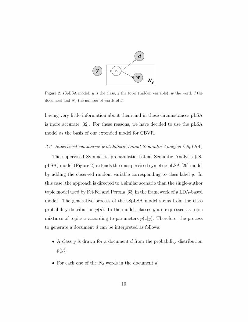
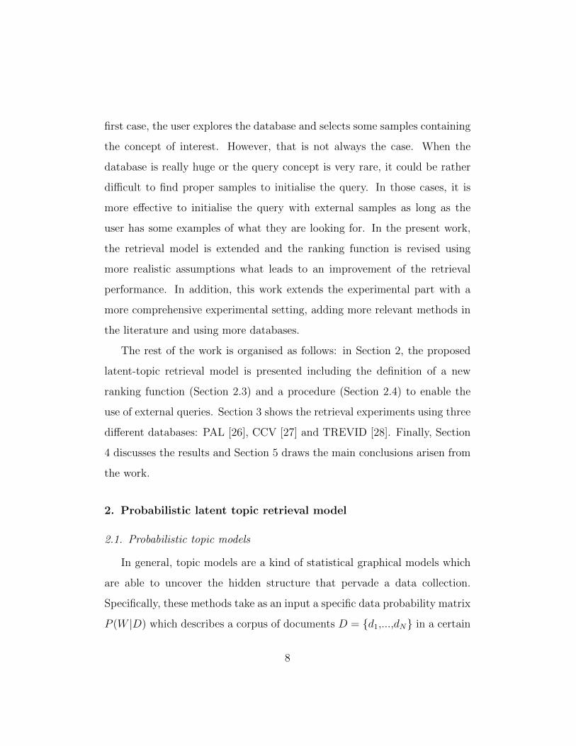
Figure 2: sSpLSA model. y is the class, z the topic (hidden variable), w the word, d the

document and Nd the number of words of d.

having very little information about them and in these circumstances pLSA

is more accurate [32]. For these reasons, we have decided to use the pLSA

model as the basis of our extended model for CBVR.

2.2. Supervised symmetric probabilistic Latent Semantic Analysis (sSpLSA)

The supervised Symmetric probabilistic Latent Semantic Analysis (sS-

pLSA) model (Figure 2) extends the unsupervised symetric pLSA [29] model

by adding the observed random variable corresponding to class label y. In

this case, the approach is directed to a similar scenario than the single-author

topic model used by Fei-Fei and Perona [33] in the framework of a LDA-based

model. The generative process of the sSpLSA model stems from the class

probability distribution p(y). In the model, classes y are expressed as topic

mixtures of topics z according to parameters p(z|y). Therefore, the process

to generate a document d can be interpreted as follows:

• A class y is drawn for a document d from the probability distribution

p(y).

• For each one of the Nd words in the document d,

10

– Given the document class y, a topic z is chosen according to con-

ditional distribution p(z|y) that expresses classes in topics.

– Given the topic z chosen, a word w is drawn from the conditional

distribution p(w|z) that relates topics to words.

• Given theNd topics drawn to extract the words, a document d is defined

according to the class conditional distribution p(d|z).

The sSpLSA model could be used to extract the topics of a data collection

using information about class labels (y) like a regular supervised topic model

but it is not the goal here. We aim at relating the sSpLSA general model

(Fig. 2) to the RF retrieval scheme (Fig. 1) in order to obtain a probabilistic

ranking function based on sSpLSA. For that purpose, we use the following

notation: y′ is the query class and represents the kind of videos the user

wants to extract from the database and D′ = {d′1,...,d′N ′} refers to the query

set containing one or more positive examples of the query class. Note the

difference between y and y′. The former (y) is related to the general concept

of class label information used in the sSpLSA model and the latter (y′) is

the specific kind of videos the user wants to extract from the database in a

specific retrieval session. Our objective is to sort the database using as a score

of the ranking the probability that each document d of the database belongs

to the query class y′, i.e. p(y′|d). In the next section, we are going to deduce

the ranking function of the proposed approach deriving this probability over

the sSpLSA model.

11

2.3. Latent Topic Ranking (LTR)

Initially, we assume that a topic process has been carried out over the

database in order to extract a specific number of topics (K) and to express

the whole collection according to those extracted topics as P (Z|D). For the

topic extraction task, it can be used either a supervised model (sLDA...) or

unsupervised (LDA, pLSA...) one. It should be noted that in the supervised

case topics are extracted using some initial class label information y which

does not have to be related to the concept y′ (query class) that the user wants

to retrieve in a particular session.

The proposed Latent Topic Ranking (LTR) function is aimed at providing

a guess of the probability p(y′|d) that each document d of the database

belongs to the query class and using these probability values it performs the

ranking at each retrieval iteration. According to the sSpLSA model (Fig. 2),

this probability can be estimated from the present user’s query by means of

topic characterisations as follows. Let us express the conditional probability

p(y′|d) by marginalising over topics:

p(y′|d) =p(y′,d)

p(d)=

∑w

∑z

p(w,d,z,y′)

p(d)=

∑w

∑z

p(w|z)p(d|z)p(z|y′)p(y′)

p(d)(1)

Where it has been assumed that the joint probability p(w,d,z,y′) is ex-

pressed according to the introduced sSpLSA model. Regarding the con-

ditional topic probability of a given class p(z|y′), it can be estimated by

marginalising over the query set D′ = {d′1,...} as follows:

12

p(z|y′) =∑d′

p(z,d′|y′) =∑d′

p(z|d′,y′)p(d′,y′)p(y′)

=∑d′

p(z|d′,y′)p(y′|d′)p(d′)p(y′)

(2)

Inserting (2) in (1) we obtain

p(y′|d) =

∑w

∑z

p(w|z)p(d|z)∑d′

p(z|d′,y′)p(y′|d′)p(d′)

p(d)(3)

The conditional probability p(y′|d′) represents the probability that a doc-

ument of the query belongs to the query class which is always true, therefore

p(y′|d′) = 1. Moreover, assuming the normalisation constraint over topics∑wp(w|z) = 1, expression (3) can be simplified as follows:

p(y′|d) =

∑z

p(d|z)∑d′

p(z|d′,y′)p(d′)

p(d)(4)

After multiplying and dividing by p(z) and applying Bayes’ rule p(z|d) =

p(d|z)p(z)/p(d) we obtain

p(y′|d) =∑z

p(d|z)p(z)

p(d)p(z)

∑d′

p(z|d′,y′)p(d′) =∑z

p(z|d)

p(z)

∑d′

p(z|d′,y′)p(d′) (5)

Let us assume that the probability p(d) of the documents of the database

and the probability p(d′) of the documents of the query follows the same uni-

form distribution over the total number of documents of the database |D|, i.e.

p(d) = p(d′) = 1/|D|. This assumption implies that all the documents have

the same prior probability independently of their number of words, features

or even their relation with other samples. In the case of internal queries,

13

it makes sense to use 1/|D| as an estimation of p(d′) because queries are

selected from the own database. Besides, even in the case of external queries

the number of samples from outside the database is so reduced compared

with the number of documents in the database (|D′| << |D|) that the value

1/|D| is a good approximation to 1/(|D|+ |D′|). Thus, p(z) can be estimated

by marginalising the documents di of the database and using Bayes’ rule

p(z) =∑di

p(z,di) =∑di

p(z|di)p(di) ≈1

|D|∑di

p(z|di) (6)

Inserting (6) into (5), the probability p(y′|d) can be expressed as

p(y′|d) ≈∑z

p(z|d)∑dip(z|di)

[∑d′

p(z|d′,y′)

](7)

In the present work, we have considered a short-term RF scheme what

means that each retrieval session is independent from one another. In other

words, all the information we have about the query class y′ is provided by the

samples of the query set d′, therefore y′ ≈ d′ and then p(z|d′,y′) ≈ p(z|d′).

As a result, the final expression to estimate the probability p(y′|d) for the

LTR function is as follows:

p(y′|d) ≈∑z

p(z|d)∑dip(z|di)

[∑d′

p(z|d′)

](8)

Expression (8) has two main factors. The left one is related to the docu-

ment d of the database we want to rank and the right factor represents the

query at a specific stage of the retrieval process. In the first factor, p(z|d) is

learned off-line using any latent topic algorithm, for instance pLSA or LDA.

Then,∑

dip(z|di) can be precomputed off-line as well using all the documents

14

of the database. In the second factor, p(z|d′) is the probability that a given

query document d′ belongs to the topic z.

The ranking process is made as follows. First of all, K topics are ex-

tracted from the database using some topic extraction method and subse-

quently each document d of the database and the initial query documents

d′ are represented in these topics as p(z|d) and p(z|d′) respectively. Later,

the database is sorted according to the probability that documents d belong

to the query class y′ using equation (8). Following the relevance feedback

scheme, the S most likely samples (scope) are showed to the user who se-

lects the P correctly retrieved samples. Then, these P samples are used as

feedback to expand the query. At each iteration, the query is expanded with

more positive examples and probabilities p(y′|d) are recomputed to refine the

ranking. In the end, the interactive process ends after I iterations when the

user has retrieved enough samples.

Comparing the LTR function (8) with the version in [23], we can observe

two main differences. On the one hand, in LTR documents are normalised by

the global use of the topics in the collection, therefore the least used topics

are able to generate a higher probability values. That is, the match with

the query patterns is calculated by fostering the least used topics. On the

other hand, expression (8) uses p(z|d′) (query expressed in topics) instead of

p(d′|z) (topics expressed in query documents). This allows to get rid of the

simplification we made in the ranking process of [23] where we assumed that

topics do not depend on queries to approximate p(d′|z) as the transposed

and normalised version of p(z|d′) what is not a real premise.

Another important change is based on allowing the use of internal and

15

Figure 3: Graphical model representation of the aspect model in the asymmetric pLSA

parametrization used by Hofmann in [29]. d is the document, z the topic (hidden variable),

w the word and Nd the number of words of d.

external query samples. The off-line topic learning process obtains P (W |Z)

and P (Z|D) from the database. Thus, when queries are inside the database,

we already have the description of the query documents in topics. However,

when queries are initialised with external samples, we have to use an es-

timation procedure to represent those external documents in the previously

extracted topics. The following section shows the used procedure to represent

external samples in a set of given topics.

2.4. Expectation Maximisation eStimator (EMS)

As it was mentioned earlier, regular topic algorithms such as pLSA and

LDA are able to obtain from a data collection the description of topics in

words as P (W |Z) and the representation of the database in topics as P (Z|D).

However, in this work queries can be initialised with samples from outside

the database and therefore the proposed approach requires an additional

procedure to represent external query documents D′out = {d′out1 ,...} in a given

set of topics as P (Z|D′out). Following the same notation than before, the

upper-case letter represents the set and the lower-case an instance of that

set.

We use the asymmetric version pLSA model (Fig. 3) to define the Ex-

pectation Maximization eStimator (EMS) procedure. Specifically, the pa-

16

rameter p(z|d′out), which represents an external query document in a given

set of topics, can be estimated following the pLSA model by maximizing the

log-likelihood using the Expectation-Maximization (EM) algorithm. Let us

define the joint distribution of the model Eq. (9) and the log-likelihood Eq.

(10) in terms of the joint probability distribution

p(w,z,d′out) = p(w|z)p(z|d′out)p(d′out) (9)

L =∑w

n(w,d′out)log[p(w,d′out)] (10)

Where n(w,d′out) is the number of occurrences of the word w in the doc-

ument d′out. In order to maximize the log-likelihood by EM, the complete

log-likelihood can be expressed using the latent variables z as

E =∑w

n(w,d′out)

(∑z

p(z|w,d′out)log[p(w|z)p(z|d′out)p(d′out)]

)(11)

Introducing in expression (11) the normalisation constraints of the pa-

rameter p(z|d′out) by inserting the appropriate Lagrange multiplier β:

H = E + β

[1−

∑z

p(z|d′out)

](12)

Taking the derivative with respect to p(z|d′out), setting the expression

equal to zero and solving the equation to isolate the parameter, the M-step

of the EM algorithm is expressed as

p(z|d′out) =

∑w

n(w,d′out)p(z|w,d′out)∑z

∑w

n(w,d′out)p(z|w,d′out)(13)

17

Figure 4: Proposed approach scheme. K (number of topics), Q (number of samples to

initialise the query), I (number of feedback iterations) and S (number of top ranked

samples).

For the E-step, we need to estimate the parameter p(z|w,d′out). Applying

the Bayes’ rule and the chain rule we obtain

p(z|w,d′out) =p(w,z,d′out)

p(w,d′out)=

p(w|z)p(z|d′out)∑z

p(w|z)p(z|d′out)(14)

The EM process is performed as follows. First of all, the external query

document n(w,d′out) and the set of previous topics p(w|z) are loaded. Sec-

ondly, p(z|d′out) is randomly initialised. Then, the E-step Eq. (14) and the

M-step Eq. (13) are alternated until a convergence condition is reached. As

default settings, we have used a threshold of 10−6 in the difference of the

log-likelihood Eq. (10) between two consecutive iterations and a maximum

of 1000 EM iterations to assure a fixed and sensible computational cost in

the convergence process.

2.5. Latent Topic-based Relevance Feedback Framework

The proposed retrieval approach is made up of three main phases (Fig.

4): (i) off-line topic extraction, (ii) on-line query definition and (iii) on-

18

line retrieval and relevance feedback. In the first phase (i), the LDA [30]

algorithm is used over the collection in order to extract K topics as P (W |Z)

and to represent the samples of the database in those topics as P (Z|D). Note

that P (W |D) represents the normalised word count of the documents of the

collection. We have selected LDA instead of pLSA because the spatial cost of

pLSA for the tested collections is unaffordable, however pLSA or any other

topic model can be used in this phase instead. Once this off-line process has

been carried out the system changes to the on-line mode which contains two

more phases.

The phase (ii) on-line query definition is corresponded to the Stage 0

of the RF scheme showed in the Fig. 1. In this part, the user has two

different alternatives to initialise the query. When queries are from inside the

database, Q query samples are selected from the own collection as the initial

query set and the rest of the samples make the Rest set which is the basis

to perform the ranking. When queries are from outside, the EMS function

is used to represent the external query samples n(w,d′out) in the previous K

extracted topics P (W |Z). Note that n(w,d′out) represents the word count of

the external query documents. Then, these external samples expressed in

topics p(z|d′out) make the Query set and the whole database P (Z|D) is used

as the Rest set. The external samples have to be represented in the same

initial characterisation space W than the database used to extract the topics

e.i. using the same descriptor.

Once the Query and Rest sets are initialised, the proposed approach

changes to the phase (iii) on-line retrieval and relevance feedback which rep-

resents the stages 1 and 2 of Fig. 1. In this iterative stage, the LTR function

19

uses both the Query and Rest sets to obtain a ranking of Rest by using

equation (8). From this ranking, the S top samples are shown to the user

who selects the positive samples to provide the feedback. These correctly re-

trieved samples are used to expand the Query and besides they are removed

from the Rest set. In order to reduce the complexity of the interaction pro-

cess, only positive feedback samples are used to expand the query. Finally,

with the updated Query and Rest sets the next iteration is triggered. The

number of total feedback iterations I depends on the user, that is, the user

decides when the interaction ends.

3. Experiments

This section presents the experimental part of the work. Section 3.1

describes the kind of retrieval simulations performed in the experiments and

the retrieval methods of the literature used to test the proposed approach.

Subsequently, sections 3.2, 3.3 and 3.4 show the retrieval results for three

different databases: PAL [26], CCV [27] and TRECVID 2007 [28].

3.1. Short-term Relevance Feedback simulations

A total of six different user interaction scenarios are defined to evaluate

the effectiveness of the proposed approach with respect to seven different

retrieval methods over three databases. We assume that each database used

for the simulations is a pre-labelled collection, i.e. it is annotated according

to a specific set of classes, and besides it is partitioned in two balanced halves,

training and test.

20

3.1.1. Parameters of the simulations

Following the scheme of the proposed approach (Figure 4), the on-line

stage has three main parameters: Q the number of samples of the initial

query, S the number of top examined items and I the number of total it-

erations. The target of each simulation is directed to retrieve samples of a

specific class, but without using any class label information. In other words,

the query is initialised with Q samples of a single class c and the simulation

process has to retrieve samples of that class through I feedback iterations. At

each iteration, the S top ranked items are inspected by a simulated user who

marks the samples of the class c (positive samples). These positive samples

are computed as correctly retrieved samples and they are used to expand the

query. Finally, the expanded query is triggered as a new query for the next

iteration.

In this work, we assume a simulated-user reliability of a 100% in order to

simplify, but some uncertainty could be introduced in the simulation process.

This uncertainty could be introduced into the retrieval system in a soft way

or in a more intense way. An example of the former case could be by limiting

the number of feedback examples per iteration. That is, instead of selecting

all the positive examples each feedback iteration just marking a few correctly

retrieved samples. Note that, this is a quite common situation because real

users do not often analyse the whole content of a screen. Another example of

a more aggressive uncertainty could be by introducing some mistakes in the

feedback process. This fact may produce a remarkable precision drop and

its study would be interesting to test the stability of the different retrieval

methods.

21

The experiments are divided in two kinds of simulations according to

the initialisation of the query (Fig. 4): (a) when queries are from inside

the database and (b) when queries are from outside the database. In the

first case (a), the complete dataset is used to extract K topics by LDA and

then for each class c of the database queries are initialised with Q random

samples of the that class. This random initialisation is repeated R times in

order to obtain an average value of the retrieval precision and an average

computational time per query. Note that by complete dataset we mean the

union of both partitions training and test because we assume that the dataset

is initially divided into these two balanced partitions.

When queries are from outside the database (b), the training partition is

used to extract K topics using LDA and the test set is represented according

to those topics by means of the EMS function. Then, each sample of the test

set is used to trigger an external query and therefore the target is to retrieve

videos from the training set which belong to the same class as the query

sample of test set. Note that in this case there is no point in considering

the parameter R because each test sample is a query itself, thus there is not

random initialisation. Like in the previous case, the performance measures

of the simulations are the average precision and average computational time

per query.

Table 1 shows the six different simulations considered for the experiments.

Those parameters have been set taking into account the user comfort in the

retrieval process. For real users, it is not comfortable to initialise the query

with many samples and for that reason we assume that the user only provides

one or two examples, that is, Q = {1,2}. The number of feedback iterations

22

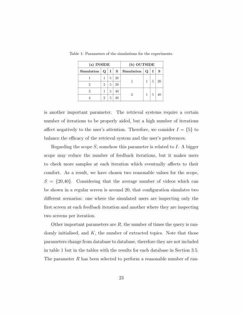
Table 1: Parameters of the simulations for the experiments.

(a) INSIDE (b) OUTSIDE

Simulation Q I S Simulation Q I S

1 1 5 201 1 5 20

2 2 5 20

3 1 5 402 1 5 40

4 2 5 40

is another important parameter. The retrieval systems require a certain

number of iterations to be properly aided, but a high number of iterations

affect negatively to the user’s attention. Therefore, we consider I = {5} to

balance the efficacy of the retrieval system and the user’s preferences.

Regarding the scope S, somehow this parameter is related to I. A bigger

scope may reduce the number of feedback iterations, but it makes users

to check more samples at each iteration which eventually affects to their

comfort. As a result, we have chosen two reasonable values for the scope,

S = {20,40}. Considering that the average number of videos which can

be shown in a regular screen is around 20, that configuration simulates two

different scenarios: one where the simulated users are inspecting only the

first screen at each feedback iteration and another where they are inspecting

two screens per iteration.

Other important parameters are R, the number of times the query is ran-

domly initialised, and K, the number of extracted topics. Note that those

parameters change from database to database, therefore they are not included

in table 1 but in the tables with the results for each database in Section 3.5.

The parameter R has been selected to perform a reasonable number of ran-

23

dom initialisations of the query to obtain robust average values. Regarding

the number of topics, selecting the right number of topics is an open-ended

issue, especially in the visual domain. In the literature, there are several ap-

proaches which try to tackle this problem but all of them require performing

the topic extraction process several times which makes them impractical to

be used in a real system. As a result, we have tested different number of

topics according to the size of the databases to make the results consistent.

3.1.2. Retrieval methods for comparison

In order to evaluate the proposed approach, we have compared our method

with seven different ranking functions. These functions have been selected

because they are widely used in literature and they usually obtain a good

performance in retrieval or classification tasks. In this work, we have used a

short-term Relevance Feedback approach, thus simulations do not use train-

ing information of previous searches. Other important retrieval approaches

need search examples as training set. Ranking SVM [34] is a powerful tool for

optimising the similarity function of content-based retrieval systems, but it

needs a reasonable training set to carry out the ranking. In the experimental

comparison, we have only used retrieval methods suitable for a short-term

Relevant Feedback scheme like the proposed approach. Specifically, we have

considered distance-based and transductive-based ranking methods for the

experiments.

The following distance/similarity ranking functions [35] have been tested:

Euclidean distance (EC), symmetric Kullback-Leibler divergence (KL), Co-

sine similarity (CS), Hellinger distance (HL) and Bhattacharyya distance

(BC). These functions have been used on the original BoW representation

24

of the dataset P (W |D) and besides on the topic space generated by LDA

P (Z|D) in order to compare the retrieval performance in both cases. The

distance/similarity based ranking sorts the samples of the database according

to the minimum distance or maximum similarity to the query. In the case

that the query has more than one sample we have computed the arithmetic

mean of the measure. Specifically, we have chosen this averaging strategy

rather than a max pooling one because in CBVR the user’s initialisation and

feedback are too limited to take advantage of sub-sampling the query set.

Regarding the transductive learning, we have selected MR (Manifold

Ranking [13]) and LRGA (Local Regression and Global Alignment [14]) as

two of the most important retrieval algorithms. However, LRGA suffers from

a high computational cost when it is used over a large number of samples

with high dimensionality. For this reason, we found that LRGA was not com-

putationally affordable for the considered databases and therefore we have

only tested MR ranking in both spaces P (W |D) and P (Z|D).

Additionally, we have tested another method in P (Z|D). Zhang et al. [15]

presented an image retrieval system which uses the cosine similarity function

in the topic space to rank the database. It uses positive and negative sam-

ples in the Relevance Feedback (RF) process and summarises the query set

in only one sample in the initial representation space P (W |D). Then, this

sample is represented as p(z|d) according to the topics extracted from the

database and eventually the cosine similarity is computed in the topic space

to perform the ranking. For comparison purposes, we have adapted this ap-

proach to the framework used in this work in order to deal with only positive

feedback. Algorithm 1 shows the Zhang (ZH) ranking function adapted for

25

the experiments.

Algorithm 1: RankingFunction of Zhang simulations.

input: QUERY , REST

size = |QUERY |;

pos = 1size

∑d∈QUERY p(w|d);

Determine p(z|pos) with EM [15];

for video v in REST do

Compute Cosine similarity between p(z|pos) and v;

end

Rank REST according to maximum similarity;

3.2. Productive Ageing Lab (PAL) database

The Productive Ageing Lab (PAL) face collection [26] contains 573 colour

images of size 640 × 480 pixels corresponding to 223 males and 350 females

with ages ranging from 18 to 93. The dataset has been randomly split into

two balanced partitions, one for training with 112 males and 175 females and

another for test with 111 males and 175 females. As a characterisation of the

data, we have used the images converted into grey levels, scaled to 16 × 13

pixels and vectorised. As a result, the original feature space P (W |D) of this

database contains 208 words.

We first use this dataset to find out easily the differences among the out-

put rankings obtained by the tested retrieval methods. Gender recognition

is a 2-class problem with a wide intra-class variety, i.e. two very different

faces could belong to the same gender, and this fact may easy the task to

detect small ranking differences. Note that the gender recognition problem

26

is extensively studied in the literature and the objective here is not to obtain

a good accuracy but to compare the different output rankings.

3.3. Columbia Consumer Video (CCV) database

The Columbia Consumer Video (CCV) dataset [27] contains 9317 YouTube

videos over 20 semantic categories, most of which are complex events, along

with several objects and scenes. The authors of the database provide two

balanced partitions, one for training with 4659 samples and another for test

with 4658 samples. Besides, they provide three different video descriptors

SIFT, STIP and MFCC. For the experiments, we have used the characterisa-

tion based on the SIFT descriptor which contains 5000 words. In particular,

this codification is made up of the concatenation of five different parts: (1)

the complete sample and (2)-(5) the division of the sample in a 2 × 2 grid.

Each one of these parts is encoded using 1000 words as the concatenation

of two different vocabularies: (a) BoW with 500 clusters over SIFT descrip-

tor and Hessian-Affine detector and (b) BoW with 500 clusters over SIFT

descriptor and DoG detector.

In this corpus, we have detected some samples with null descriptor con-

tent and others without annotation. In both cases these samples have been

removed for the experiments. For the remaining ones, those samples labelled

with more than one category have been replicated one for each class. As a

result, we have considered a total of 7846 video samples, 3914 of training and

3932 of test, annotated in 20 classes as it is shown in Fig.5.

27

Figure 5: Samples per class of the CCV database.

3.4. TRECVID 2007 database

The TRECVID 2007 collection [28] is made up of 47,548 video shots which

are annotated according to 36 semantic concepts. These categories were

selected in TRECVID 2007 evaluation and they include several objects as

well as complex events and scenes. Regarding the description of the database,

we have used a similar characterisation than in the case of CCV. Specifically,

we have followed the suggestions of van de Sande et al. [36] about using

opponent SIFT histograms when choosing a single descriptor and no prior

knowledge about the dataset is considered. The software provided by van de

Sande has been applied to the middle frame of each shot and each sample

has been encoded using a 3-level spatial pyramid codebook (1× 1, 2× 2 and

4×4) what makes a total of 2688 words per shot. In order to make affordable

the computational cost of the topic extraction task, we have reduced the

original database by selecting a balanced subset with a similar size to the

CCV collection. Specifically, we have divided the whole collection in 10

balanced partitions. Later, we have removed the classes under 100 samples

in any partition, resulting a total of 17 selected classes. Finally, we have

28

Figure 6: Samples per class of the considered subset of TRECVID 2007.

chosen one random partition as a training set and another as a test. Figure 6

shows the considered subset of 8974 samples with 4487 for training and 4487

for test annotated in 17 classes.

3.5. Results

Tables 2, 3 and 4 present the retrieval result in terms of Average Precision

(AP) and average computational Time per query in seconds (T) running in a

single processor Intel Xeon E5-2640. Each table corresponds to a particular

database and the way they are organised is the following. In columns we have

the six different simulations described in section 3.1, the first four (a) using

internal queries and the last two (b) with external ones. The parameters of

each simulation (R,Q,I,S) are indicated in the headings of the columns. In

rows we have the different retrieval methods used for the experiments. In

particular, there are three groups: LTR which contains the results of the

proposed approach using several number of topics (K), P (W |D) which has

the results of six different ranking functions in the original characterisation

space and P (Z|D) contains the results of seven different ranking functions

in the best topic space among the tested number of topics.

29

Related to the ranking functions, we use the following terminology: Eu-

clidean distance (EC), symmetric Kullback-Leibler divergence (KL), Cosine

similarity (CS), Hellinger distance (HL), Bhattacharyya distance (BC), Man-

ifold ranking [13] (MF) and Zhang approach [15] (ZH).

4. Discussion

The first noteworthy point is the remarkable precision gains provided by

topic models in the performed retrieval simulations. Comparing the best

average precision value obtained in the original BoW space P (W |D) with

the best value among the seven ranking functions tested in the topic space

P (Z|D), we observe that in the topic space the precision is increased on av-

erage a 20.35% for the PAL database, 67.14% in the case of CCV and 21.10%

for TRECVID. These significant precision gains support our statement that

the hidden patterns provided by topic models are useful to fill the semantic

gap in CBVR. Topic models have shown to help in many areas, such us text

categorisation or image recognition, but in tasks where precision is impor-

tant, like in CBVR, they have been traditionally considered useless. Some

authors have this belief because the best ranking functions in the original

BoW space tend not to work properly in the latent space. As we can see in

the results, the best ranking functions in the original BoW space are EC (for

PAL) and MF (for CCV and TREVID) but these two functions are often

two of the worse in the latent space. However, the CS function is able to

obtain a real precision improvement in the topic space. In fact, CS is the

unique function which has shown to be effective in the latent space among

the tested retrieval methods of the literature.

30

Table 2: Retrieval result for PAL database: Average Precision (AP) and average seconds

per query (T). For each group of ranking functions (in rows), the best AP value of each

simulation is highlighted in bold and the best global value among all methods is underlined.

PA

LD

AT

AB

ASE

METHOD

(a) INSIDE (b) OUTSIDE

Sim1

R=100 I=5

Q=1 S=20

Sim2

R=100 I=5

Q=2 S=20

Sim3

R=100 I=5

Q=1 S=40

Sim4

R=100 I=5

Q=2 S=40

Sim1

R=1 I=5

Q=1 S=20

Sim2

R=1 I=5

Q=1 S=40

AP T AP T AP T AP T AP T AP T

LT

R

K=20 0.5260 0.00 0.5342 0.01 0.4752 0.01 0.4872 0.01 0.4791 0.01 0.4062 0.01

K=100 0.5466 0.01 0.5419 0.01 0.4983 0.02 0.5011 0.03 0.4774 0.01 0.4187 0.01

K=200 0.5460 0.03 0.5445 0.03 0.4998 0.05 0.5059 0.06 0.4985 0.01 0.4298 0.01

P(W|D

)

EC 0.4562 0.02 0.4657 0.02 0.3954 0.04 0.3987 0.04 0.3973 0.01 0.3384 0.02

KL 0.4394 1.60 0.4400 1.86 0.3819 3.15 0.3828 3.30 0.3874 0.65 0.3273 1.05

CS 0.4495 0.04 0.4530 0.04 0.3919 0.07 0.3898 0.08 0.3919 0.02 0.3358 0.02

HL 0.4438 0.23 0.4487 0.25 0.3868 0.42 0.3897 0.39 0.3910 0.10 0.3305 0.16

BC 0.4381 0.11 0.4338 0.11 0.3817 0.18 0.3826 0.18 0.3856 0.04 0.3275 0.07

MF 0.3997 0.12 0.4169 0.13 0.3630 0.11 0.3715 0.11 0.3754 0.05 0.3305 0.05

P(Z

=20

0|D

)

EC 0.4134 0.03 0.3925 0.03 0.3306 0.04 0.3158 0.04 0.3089 0.01 0.2634 0.01

KL 0.4898 1.62 0.5104 1.91 0.4197 3.12 0.4256 1.82 0.4195 0.69 0.3479 1.06

CS 0.5462 0.03 0.5834 0.04 0.4699 0.06 0.4941 0.06 0.4656 0.02 0.3914 0.03

HL 0.5102 0.23 0.5349 0.26 0.4344 0.40 0.4446 0.39 0.4365 0.10 0.3659 0.17

BC 0.4978 0.12 0.5186 0.14 0.4194 0.22 0.4275 0.22 0.4209 0.04 0.3557 0.07

MF 0.4032 0.11 0.4312 0.11 0.3445 0.11 0.3630 0.11 0.3895 0.05 0.3405 0.05

ZH 0.3588 0.03 0.3582 0.03 0.3181 0.03 0.3173 0.03 0.4034 1.34 0.3344 1.31

31

Table 3: Retrieval result for CCV database: Average Precision (AP) and average seconds

per query (T). For each group of ranking functions (in rows), the best AP value of each

simulation is highlighted in bold and the best global value among all methods is underlined.

CC

VD

AT

AB

ASE

METHOD

(a) INSIDE (b) OUTSIDE

Sim1

R=500 I=5

Q=1 S=20

Sim2

R=500 I=5

Q=2 S=20

Sim3

R=500 I=5

Q=1 S=40

Sim4

R=500 I=5

Q=2 S=40

Sim1

R=1 I=5

Q=1 S=20

Sim2

R=1 I=5

Q=1 S=40

AP T AP T AP T AP T AP T AP T

LT

R

K=100 0.1154 0.07 0.1313 0.09 0.1136 0.13 0.1275 0.16 0.1150 0.02 0.1111 0.04

K=500 0.1496 0.39 0.1694 0.42 0.1529 0.54 0.1686 0.65 0.1473 0.14 0.1465 0.23

K=1000 0.1597 0.50 0.1810 0.58 0.1716 0.86 0.1886 0.99 0.1664 0.25 0.1667 0.41

K=1500 0.1860 1.36 0.2121 1.25 0.1935 1.82 0.2137 2.07 0.1793 0.47 0.1782 0.81

K=2000 0.1952 1.23 0.2198 1.38 0.1974 2.11 0.2163 2.37 0.1837 0.53 0.1824 0.93

P(W|D

)

EC 0.0964 3.23 0.0927 3.32 0.0786 4.35 0.0766 4.74 0.0782 1.19 0.0650 1.87

KL 0.0708 120 0.0575 108 0.0688 208 0.0617 215 0.0840 76.6 0.0697 124

CS 0.1111 3.97 0.1105 4.52 0.0924 7.27 0.0921 9.54 0.0922 1.58 0.0769 2.50

HL 0.1001 22.4 0.0974 28.3 0.0827 39.6 0.0820 40.8 0.0859 14.8 0.0693 22.9

BC 0.1005 12.7 0.0932 13.7 0.0821 20.3 0.0774 21.3 0.0838 7.04 0.0681 10.8

MF 0.1293 103 0.1390 103 0.1059 103 0.1121 103 0.1007 33.6 0.0796 33.6

P(Z

=20

00|D

)

EC 0.0710 0.84 0.0645 1.03 0.0556 1.57 0.0500 1.53 0.0433 0.28 0.0333 0.42

KL 0.1423 78.9 0.1352 85.6 0.1165 126 0.1107 132 0.1078 26.9 0.0866 43.5

CS 0.2040 2.52 0.2344 2.76 0.1789 3.94 0.1978 5.17 0.1605 0.78 0.1386 1.31

HL 0.1748 13.1 0.1848 14.7 0.1427 21.0 0.1477 23.6 0.1426 5.07 0.1110 8.24

BC 0.1684 6.46 0.1703 7.20 0.1380 10.4 0.1392 11.7 0.1361 2.43 0.1064 3.89

MF 0.1059 22.3 0.1242 22.3 0.0776 22.3 0.0889 22.3 0.0706 8.95 0.0511 8.95

ZH 0.1518 539 0.1707 538 0.1248 539 0.1371 539 0.1285 450 0.1028 449

32

Table 4: Retrieval result for TRECVID database: Average Precision (AP) and average

seconds per query (T). For each group of ranking functions (in rows), the best AP value

of each simulation is highlighted in bold and the best global value among all methods is

underlined.

TR

EC

VID

DA

TA

BA

SE

METHOD

(a) INSIDE (b) OUTSIDE

Sim1

R=500 I=5

Q=1 S=20

Sim2

R=500 I=5

Q=2 S=20

Sim3

R=500 I=5

Q=1 S=40

Sim4

R=500 I=5

Q=2 S=40

Sim1

R=1 I=5

Q=1 S=20

Sim2

R=1 I=5

Q=1 S=40

AP T AP T AP T AP T AP T AP T

LT

R

K=100 0.0920 0.08 0.0972 0.09 0.0951 0.10 0.0996 0.12 0.0867 0.02 0.0828 0.03

K=500 0.1298 0.22 0.1349 0.23 0.1366 0.28 0.1375 0.30 0.1279 0.11 0.1319 0.16

K=1000 0.1482 0.43 0.1529 0.45 0.1626 0.56 0.1666 0.60 0.1302 0.23 0.1389 0.35

K=1500 0.1547 0.64 0.1538 0.69 0.1659 0.85 0.1676 0.91 0.1331 0.35 0.1418 0.53

K=2000 0.1553 0.86 0.1595 0.93 0.1698 1.23 0.1740 1.21 0.1354 0.47 0.1435 0.70

P(W|D

)

EC 0.1100 0.73 0.1091 0.97 0.1080 1.21 0.1066 1.42 0.0692 0.58 0.0663 1.02

KL 0.1214 36.6 0.1171 45.9 0.1179 59.8 0.1162 70.5 0.0717 34.3 0.0695 50.6

CS 0.1177 0.97 0.1164 1.23 0.1130 1.58 0.1103 1.83 0.0670 0.71 0.0654 1.25

HL 0.1156 6.86 0.1111 7.41 0.1144 9.75 0.1092 11.2 0.0738 4.93 0.0710 8.90

BC 0.1141 2.93 0.1104 3.67 0.1139 4.75 0.1083 5.39 0.0733 2.41 0.0709 4.66

MF 0.1521 47.7 0.1365 47.5 0.1332 47.6 0.1158 47.9 0.1046 3.72 0.0791 3.72

P(Z

=20

00|D

)

EC 0.1001 0.52 0.0962 0.67 0.0957 0.82 0.0906 0.97 0.0979 0.60 0.0914 0.80

KL 0.1272 32.7 0.1248 40.5 0.1233 53.7 0.1204 62.1 0.1069 34.3 0.1014 50.6

CS 0.1523 0.72 0.1603 0.97 0.1547 1.22 0.1556 1.45 0.1278 0.62 0.1253 1.10

HL 0.1322 4.95 0.1313 6.14 0.1261 7.95 0.1252 9.32 0.1132 4.34 0.1066 7.81

BC 0.1298 2.48 0.1293 3.12 0.1247 3.97 0.1234 4.63 0.1116 3.72 0.1057 3.84

MF 0.1441 37.1 0.1229 37.1 0.1320 37.1 0.1155 37 0.0929 2.87 0.0556 2.87

ZH 0.1161 266 0.1276 280 0.1069 275 0.1148 267 0.0976 305 0.0840 314

33

Another noticeable question related to the latent space is the adequate

number of topics. We have tested several values for each database and the

best precision results are obtained using the highest numbers, that is, 200

topics for PAL database and 2000 for both CCV and TRECVID. However, for

PAL and TRECVID the precision improvement using these values is quite

slight compared with the results obtained with 100 and 1500 respectively.

This indicates that, depending on the database and the kind of queries,

increasing the number of topics reaches a point in which it does not provide

an actual improvement. Selecting the appropriate number of topics is an

important question and still remains an open-ended issue in the literature.

Even though the number of topics may significantly affect to the performance

of a system, for this kind of application it is more important to have enough

topics to obtain a fine granularity of patterns to describe queries than to

find out exactly the optimum number. Somehow, it is similar to the case of

finding the optimum number of clusters in a classification problem. As long

as you have enough clusters to represent the classes it is not so important if

some classes are represented with more than exactly one cluster.

In general, the results show a similar trend in the three tested databases.

The LTR function achieves the best retrieval precision on average compared

with the best methods in both the original BoW space P (W |D) and the

latent space P (Z|D). In the PAL database, LTR outperforms EC-pwd in a

23.38% and CS-pzd in a 2.52%. For CCV, the precision gain of LTR is a

79.19% over MF-pwd and a 7.22% over CS-pzd. In the case of TRECVID,

LTR increases the precision of MF-pwd in a 29.58% and the precision of

CS-pzd in a 7.00%.

34

Related to the parameters of the simulations, we observe the that average

precision tend to increase using a bigger Q (number of samples to initialise

queries) and it drops with a larger value of S (scope). The rationale behind

this is the following: on the one hand, initialising queries with more samples

provides more information about the concept of interest and then the retrieval

systems is more effective. On the other hand, considering a larger scope

makes the retrieval system use more samples which are less likely to belong

to the query class what eventually generates a precision drop.

According to the results, the proposed LTR shows a good robustness

regarding the parameters Q and S of the simulations. Focusing on CCV and

TRECVID, the proposed LTR method obtains a similar precision gain to

the best tested function (CS-pzd) when the parameter Q increases (Sim2-

inside and Sim4-inside). In addition, LTR is able to reduce the precision

drop compared with CS-pzd when the parameter S is increased (Sim3-inside,

Sim4-inside and Sim2-outside).

The proposed LTR function is able to outperform the tested methods in

the original BoW space and in the latent space with the exception of CS-pzd.

For that reason, we discuss in more detail the differences between LTR and

CS to highlight the advantages of the proposed approach.

4.1. Cosine Similarity (CS) vs. Latent Topic Ranking (LTR)

The CS function uses the cosine of the angle between two samples as

a similarity measure. That is, the most similar documents to the query

are those which have the lowest angle with respect to the query (angular

similarity). In the case the query has more than one document, we have

used the average cosine similarity value. Equation (15) shows the CS function

35

where d represents a document of the database and D′ the query set.

Sim(d,D′) =

∑d′∈D′

cos(θd,d′)

|D′|=

∑d′∈D′

d · d′

|d||d′|

|D′|(15)

The proposed LTR function provides a probabilistic approach to discover

the most likely samples according to the query. As it is shown in equation

(16), this function can be interpreted as a weighted scalar product between

the document d and a summary of the query set in a single document. The

topics weights are computed as the inverse of the prior of each topic in the

database. Therefore, the least used topics generate higher probability values,

that is, the LTR function is a weighted scalar product which fosters the least

used topics in the database. Intuitively, this makes sense because the least

used patterns may allow us to discriminate better among samples for complex

query concepts.

LTR(d,D′) =∑z

(1∑

dip(z|di)

)︸ ︷︷ ︸

topic weight

weighted scalar product︷ ︸︸ ︷(p(z|d))︸ ︷︷ ︸document

(∑d′∈D′

p(z|d′)

)︸ ︷︷ ︸

query summary

(16)

At the same time, the scalar product (dot product) between two vectors

is directly proportional to the projection of the first on the second vector.

That is, (d · d′) = |d′| Projectiond−d′ . Logically, cosine similarity and LTR

function have some similar features because the less angle often implies the

more projection and then the more scalar product value. However, there is

a main difference which enables the LTR function to overcome the cosine

similarity retrieval precision. The weighting scheme gives more flexibility to

36

Figure 7: Example of gender retrieval. Cosine and LTR rankings at the first iteration

with a scope of 20. The figure only shows the images which are different in both 20-top

rankings (8 pictures). The images are sorted from left to right according to the original

20-top ranking order.

the LTR function in order to deal with the semantic gap challenge.

Comparing both behaviours, the LTR function selects the documents

within a margin of larger weighted scalar projection by fostering the least

used topics. In a real application, this produces a top ranking with more

variety of documents and then the user’s feedback is able to provide more

relevant information about the scope of the query concept. Let us see it

through an example of gender retrieval using the PAL database. We are

going to use an initial query of an elderly woman to compare the LTR and

CS rankings at the first ranking iteration. Assuming queries from inside the

PAL database, Figure 7 shows the differences between both 20-top rankings

at the first iteration. The shared images have been removed to highlight the

differences between the two ranking functions.

First of all, it should be noted the relationship between LTR and CS. A

total of 12 images are the same in both 20-top rankings at the first itera-

tion. Specifically, 8 white old women, 2 black women, one black man and

37

another white man are shared by both rankings. This fact clearly shows

the aforementioned relation between projection (LTR) and angular similar-

ity (CS). However, we can appreciate a very important difference between

the not overlapped images of both rankings. The cosine similarity function

tends to retrieve samples of older women (the initial query) whereas LTR

first retrieves women with different appearances. That is, the LTR function

provides a broader kind of women images, thus the proposed approach is able

to obtain a broader and more meaningful feedback about the query class.

As it was introduced in Section 1, the main problem in CBVR is the

semantic gap challenge i.e. the difference between the user’s understanding

and the data representation. In CBVR, the same video sample can be related

to very different concepts (queries) and the only way we have to distinguish

among them is by the user’s feedback. Therefore, enriching the query with a

wide variety of positive examples in the feedback is a key factor to deal with

unconstrained concepts.

Figure 8 shows the number of correctly retrieved videos per ranking it-

eration for the experiments using the CCV database. In both internal and

external queries, we can see how the CS function archives the best perfor-

mance at the first iteration and then the precision decreases in the subse-

quent iterations. However, LTR obtains the best performance at the second

iteration after the first user’s feedback and for the following iterations the

precision drop is smoother than in the case of CS. This example shows that

the feedback extracted from the LTR ranking contains a more useful infor-

mation of the query class. Even though the number of positive samples is

lower at the first iteration, the fostering of the least used topics made by LTR

38

(a) Simulations when queries are from inside the CCV database.

(b) Simulations when queries are from outside the CCV database.

Figure 8: Proposed approach (LTR) vs Cosine Similarity (CS). Average of correctly re-

trieved samples per iteration for the performed video retrieval simulations using the CCV

database.

generates a user’s feedback more meaningful because it includes samples with

a broader variety of topics related to the query. Eventually, this variety of

hidden patterns allows users to describe better the concept of interest though

the feedback they provide.

4.2. Computational complexity issues

Regarding the computational burden, the results show a high performance

of the LTR function with respect to the best tested methods in both P (W |D)

and P (Z|D) spaces. LTR can process documents faster than the methods

39

tested in the original BoW space P (W |D) because the proposed function

performs the ranking in the topic-model space P (Z|D) and this space has

usually a lower dimensionality than the former. For instance, in the CCV

simulations the original feature space with 5000 words is reduced by LDA to

a topic space with 2000 topics what means a 60% dimensionality reduction.

Comparing LTR with the methods tested in P (Z|D), the proposed function

is able to obtain a good computational time as well. Despite the fact that

EC-pzd is more efficient than LTR, the precision of the Euclidean distance

in the latent space is so poor that the single competitor of LTR is CS-pzd.

According to the results, LTR tends to outperform the computational

time obtained by CS-pzd. The proposed LTR function (Eq. (16)) summarises

the whole query set in a single document (query summary), then a single

scalar product is performed for each sample to be ranked. That is, the cost

of obtaining the score of a document is O(|D′|K + K) = O(|D′|K) where

|D′| represents the size of the query set at a specific time moment and K

the number of topics. Note that topic weights (∑

dip(z|di)) in Eq. (16) are

computed off-line. The CS function (Eq. (15)) uses the average cosine value

for all the documents of the query, therefore it needs to compute |D′| scalar

products, two magnitudes and a query cardinality per document to rank.

That makes a total cost of O(3|D′|K + |D′|) = O(|D′|K). The asymptotic

cost of both functions is the same but in practice LTR is able to achieve a

better computational time because of the multiplicative constants.

The average computational time per query shown in the results corre-

sponds to the cost of the ranking function itself, that is, the stage (iii) of Fig.

4. However, the RF scheme contains two more procedures that we should

40

Table 5: Computational time of LDA and EMS for the CCV database.

LDA (default parameters) EMS (default parameters)

CCV (tra + tst)

K Time RAM CCV - tst AVG Time per Doc EM Iters MAX Iters

100 2 days 0.40 GB P (z = 100|d′) 0.63 sec 475.55 2.23%

500 8 days 1.20 GB P (z = 500|d′) 3.68 sec 548.83 4.34%

1000 15.5 days 2.20 GB P (z = 1000|d′) 9.05 sec 662.76 5.49%

1500 23 days 3.20 GB P (z = 1500|d′) 15.24 sec 668.72 6.26%

2000 30.5 days 4.20 GB P (z = 2000|d′) 22.31 sec 711.14 6.94%

take into account: LDA in stage (i) and EMS in (ii). Table 5 presents the

computational time of both procedures for the CCV database. In the case of

LDA, we use a parallel version running in 24 Intel Xeon E5-2640 processors

and in the case of EMS a single processor Intel Xeon E5-2640. As we can see,

the topic extraction task is a very time-consuming process. Although LDA

runs off-line, its cost may limit its usage in much larger databases. However,

the proposed LTR function is independent of the topic extraction algorithm,

therefore further improved methods could be used instead of LDA.

Related to the EMS function, the more topics the more costly the process.

In the case of CCV, the average time to represent an external query document

in 2000 topics is over 20 seconds what seems noticeable higher compared with

the costs of the ranking functions. However, this cost has to be taken as a pre-

processing step although it is part of the ON-LINE - Query Definition stage.

In the case of external queries, a pre-processing step is always required to

represent those external samples in the same way the database was encoded

in visual Bag of Words. Finally, note that these computational disadvantages

of LDA and EMS are not exclusive for the proposed LTR function but for

all the retrieval methods running in latent topic spaces.

In addition to computational time, Table 5 shows the convergence average

41

values of the EMS function for the CCV database. As we can see the average

number of EM iterations per document is below the considered default limit

of 1000 and besides there is a small percentage of documents which actually

reach this limit in the convergence process.

4.3. Limitations of the proposed approach

Although the presented LTR function has shown to outperform the rest of

the tested methods, there are two points which have to be taken into account:

(i) the topic extraction cost and (ii) the patterns diversity provided by LTR.

Related to the first point, current topic extraction algorithms are still very

costly and more research in that field is required to enable processing video

collections with millions of videos. This is is not a limitation specifically of

LTR but it is a drawback of all the ranking functions working in the latent

topic space. However, the proposed approach has been designed isolating

the off-line topic extraction process from the on-line retrieval task. This

makes that further improvements on the topic extraction methods can be

directly used by replacing LDA to extract the topics. The second point to be

considered is the patterns diversity provided by LTR. The proposed retrieval

approach has been designed assuming a wide semantic gap to deal with by

means of a RF scheme, that is the typical situation in CBVR. As we have

shown, the topic diversity provided by LTR at the top-ranking is able to

provide a competitive advantage because it may obtain a more informative

feedback. However, this diversity is only useful when there is feedback itself

because the user discards those samples related to useless patterns. That

limits the effectiveness of LTR in those situations where there is not feedback

at all. As we can see in Fig. 8, the precision gains of LTR over CS are

42

obtained after the first user’s feedback. That is, CS obtains a better precision

than LTR at the first ranking iteration where there is not feedback just the

query initialisation.

5. Conclusions

In this work, we have presented a novel interactive retrieval approach ad-

dressing the retrieval problem as a class discovery problem using latent top-

ics. The sSpLSA model has been introduced to deduce the LTR probabilistic

ranking function and the EMS procedure has been defined to enable exter-

nal queries. Later, we have defined the proposed retrieval framework based

on short-term relevance feedback. Finally, several retrieval simulations have

been performed using three different datasets (PAL, CCV and TRECVID)

and several of the most relevant retrieval methods in the literature.

One of the main conclusions that arises from the work is the importance of

topic models to deal with the semantic gap in CBVR. Although topic models

have shown to be helpful in many areas, they have not been traditionally

considered useful in CBVR because of the special nature of the latent space.

However, this work shows that (i) the hidden patterns defined by topics can

be effectively used in video retrieval tasks and (ii) the proposed LTR ranking

function is able to outperform the rest of the tested functions mainly because

it has the same probabilistic nature than topic models.

The results of the work provide evidences about the viability of the pro-

posed approach in terms of effectiveness and efficiency to deal with the se-

mantic gap challenge in the CBVR field. In this domain, two users could

provide the same query initialisation but referring to two different query

43

concepts because each one is focusing on a different aspect. As a result, the

feedback quality is an essential issue to find out about the query concept. As

we have shown, the proposed LTR function promotes the least used topics

and then it enriches the top-ranking with a more variety of related hidden

patterns what eventually produces a more meaningful feedback.

Although results are encouraging, much more progress is needed to really

address the semantic gap problem which involves several fields, from low level

descriptors to high level understanding and user interaction. Specifically,

further work is directed to extend the work in the following directions:

• Automatic strategies to set the most appropriate number of topics.

• Extension of the retrieval model to a long-term RF approach.

• Reduction of the computational time of the topic extraction task by

applying quantisation methods in the initial object (video) space.

References

[1] S. Antani, A survey on the use of pattern recognition methods for

abstraction, indexing and retrieval of images and video, Pattern Recog-

nition 35 (2002) 945–965.

[2] A. F. Smeaton, Techniques used and open challenges to the analysis,

indexing and retrieval of digital video, Information Systems 32 (2006)

545–559.

[3] Y. Liu, D. Zhang, G. Lu, W.-Y. Ma, A survey of content-based image

retrieval with high-level semantics, Pattern Recognition 40 (2007) 262–

282.

44

[4] D. Zhang, M. M. Islam, G. Lu, A review on automatic image annotation

techniques, Pattern Recognition 45 (2012) 346–362.

[5] G. Chechik, V. Sharma, U. Shalit, S. Bengio, Large scale online learn-

ing of image similarity through ranking, Journal of Machine Learning

Research 11 (2010) 1109–1135.

[6] G.-H. Liu, Z.-Y. Li, L. Zhang, Y. Xu, Image retrieval based on micro-

structure descriptor, Pattern Recognition 44 (2011) 2123–2133.

[7] M. Arevalillo-Herrez, F. J. Ferri, J. Domingo, A naive relevance feed-

back model for content-based image retrieval using multiple similarity

measures, Pattern Recognition 43 (2010) 619–629.

[8] R. d. S. Torres, A. X. Falcao, M. A. Goncalves, J. a. P. Papa, B. Zhang,

W. Fan, E. A. Fox, A genetic programming framework for content-based

image retrieval, Pattern Recognition 42 (2009) 283–292.

[9] W. Ren, S. Singh, M. Singh, Y. S. Zhu, State-of-the-art on spatio-

temporal information-based video retrieval, Pattern Recognition 42

(2009) 267–282.

[10] S. Tong, E. Chang, Support vector machine active learning for image

retrieval, in: ACM International Conference on Multimedia, pp. 107–

118.

[11] K. Tieu, P. Viola, Boosting image retrieval, International Journal of

Computer Vision 56 (2004) 17–36.

45

[12] Y. Jiang, S. Bhattacharya, S. Chang, M. Shah, High-level event recog-

nition in unconstrained videos, International Journal of Multimedia

Information Retrieval 2 (2013) 73–101.

[13] D. Zhou, J. Weston, A. Gretton, O. Bousquet, B. Scholkopf, Ranking on

data manifolds, in: Advances in Neural Information Processing Systems.

[14] Y. Yang, F. Nie, D. Xu, J. Luo, Y. Zhuang, Y. Pan, A multimedia re-

trieval framework based on semi-supervised ranking and relevance feed-

back, IEEE Transactions on Pattern Analysis and Machine Intelligence

34 (2012) 723–742.

[15] R. Zhang, Z. Zhang, Effective image retrieval based on hidden concept

discovery in image database, IEEE Transactions on Image Processing

16 (2007) 562–572.

[16] D. G. Lowe, Distinctive image features from scale-invariant keypoints,

International Journal of Computer Vision 60 (2004) 91–110.

[17] I. Laptev, On space-time interest points, International Journal of Com-

puter Vision 64 (2005) 107–123.

[18] C. V. Cotton, D. P. W. Ellis, Audio fingerprinting to identify multiple

videos of an event, in: IEEE International Conference on Acoustics,

Speech and Signal Processing, pp. 2386–2389.

[19] J. Sivic, A. Zisserman, Video Google: A text retrieval approach to

object matching in videos, in: International Conference on Computer

Vision, volume 2, pp. 1470–1477.

46

[20] H. Wang, C. Schmid, Action recognition with improved trajectories, in:

IEEE International Conference on Computer Vision, pp. 3551–3558.

[21] C. Snoek, M. Worring, J. Gemert, J. Geusebroek, A. Smeulders, The

challenge problem for automated detection of 101 semantic concepts in

multimedia, ACM International Conference on Multimedia (2006).

[22] A. W. M. Smeulders, M. Worring, S. Santini, A. Gupta, R. Jain,

Content-based image retrieval at the end of the early years, IEEE

Transactions on Pattern Analysis and Machine Intelligence 22 (2000)

1349–1380.

[23] R. Fernandez-Beltran, F. Pla, An interactive video retrieval approach

based on latent topics, in: International Conference on Image Analysis

and Processing, pp. 290–299.

[24] D. M. Blei, Probabilistic topic models, Communications of the ACM

55 (2012) 77–84.

[25] A. Atreya, C. Elkan, Latent semantic indexing (lsi) fails for trec collec-

tions, SIGKDD Explor. Newsl. 12 (2011) 5–10.

[26] M. Minear, D. Park, A lifespan database of adult facial stimuli, Behavior

Research Methods, Instruments, and Computers 36 (2004) 630–633.

[27] Y. G. Jiang, G. Ye, S. F. Chang, D. Ellis, A. C. Loui, Consumer video

understanding: a benchmark database and an evaluation of human and

machine performance, in: ACM International Conference on Multimedia

Retrieval.

47

[28] S. Ayache, G. Qunot, Trecvid 2007 collaborative annotation using active

learning, in: Proceedings of the TRECVID 2007 Workshop.

[29] T. Hofmann, Unsupervised learning by probabilistic latent semantic

analysis, Machine Learning 42 (2001) 177–196.

[30] D. Blei, A. Ng, M. Jordan, Latent dirichlet allocation, Journal of

Machine Learning Research 3 (2003) 993–1022.

[31] J. Chang, S. Gerrish, C. Wang, J. L. Boyd-graber, D. M. Blei, Reading

tea leaves: How humans interpret topic models, in: Advances in Neural

Information Processing Systems 22, 2009, pp. 288–296.

[32] Y. Lu, Q. Mei, C. Zhai, Investigating task performance of probabilistic

topic models: An empirical study of plsa and lda, Information Retrieval

14 (2011) 178–203.

[33] F.-F. Li, P. Perona, A bayesian hierarchical model for learning natural

scene categories, in: IEEE Computer Society Conference on Computer

Vision and Pattern Recognition, pp. 524–531.

[34] T. Joachims, Optimizing search engines using clickthrough data, in:

Proceedings of the Eighth ACM SIGKDD International Conference on

Knowledge Discovery and Data Mining, ACM, 2002, pp. 133–142.

[35] M. M. Deza, E. Deza, Encyclopedia of Distances, Springer Berlin Hei-

delberg, 2009.

[36] K. E. A. van de Sande, T. Gevers, C. G. M. Snoek, Evaluating color

48

descriptors for object and scene recognition, IEEE Transactions on Pat-

tern Analysis and Machine Intelligence 32 (2010) 1582–1596.

49