LC4

SCOF

'ELECTEIFEB 2 3 1983

DEPARTMENT OF THE AIR FORCECl- AIR UNIVERSITY (ATC)C AIR FORCE INSTITUTE OF TECHNOLOGY

Wright-Patterson Air Force Base, Ohio

___ hs d~oc'ulimnt he b,,n rppr, o.'jfo publdc r is d ,

dw!ubutuK

&PIT/GR/8U•/2D-70

/

DUAL-SEEKER MEASUREMENT PROCESSINGFOR TACTICAL MISSILE GUIDANCE

THESIS

AFIT/GE/EE/82D-70 Andrew C. Weston2Lt USAF

Approved for public release; distribution unlimited

"AIT/G/R/8 2/8D-70

DUAL-SEEKER MEASUREMENT PROCESSING

FOR TACTICAL MISSILE GUIDANCE

THESIS

Presented to the Faculty of the School of Engineering

of the Air Force Institute of Technology

Air University

in Partial Fulfillment of the

Requirements for the Degree of

Master of Science in

Electrical Engineering Access--on YorN NT111) GRA&I

TDTIc TAB

By By_Di~ti 2,ut- cde,

Andrew C. Weston, BSEE "/OrDi:,t

2Lt USAF I

December 1982

Aiproved for Public Release; Distribution Unlimited

Acknowledgements

This thesis has been perhaps the most chalienging task

I have ever faced. Understanding the theory involved;

putting the necessary work into the programmring, analysis,

and writing; and maintaining the required interest and

6,tIvaton all seernmd impnsqihl• at times and were, in

reality, beyond my capabilities alone. I recognize, and

am profoundly grateful for, the strength I have received

and the love I have felt from the Lord my God, the Father,

Son, and Holy Spirit. 4ithout Hi, help, I could never have

completed this thesis.

I also wish to extend my thanks to my advisor,

Ltc Robc-rt Edwards, foc his patience and understanding

throughout this project, and to my other committee members,

Dr. Peter Maybeck and Capt Aaron Dewispelare, for their

time and support. Thanks also goes to my sponsor,

Mr. Phil Richter of the Armament Laboratory, Eglin AFB, for

providing this interesting topic and his support. I am

also very grateful to Mr. Stan Musick of the

Avionics Laboratory, Wright-Patterson AFB, and to

Mr. Marshall Watson and Lt Scott. Trimbali of the Armament

Lab for their invaluable help on the software for this

project.

t also want to extend special thanks and recognition

to some very important people. Capts Hank Worsley and

Don stiffier gave ire immeasurable help during some of the

hardest times. They provided practical guidance and helped

me gain the insight that I needed, and I know that I could

not have achieved the satisfaction I feel towards this

thesis without them. They also provided inspiration and

encouragement when I needed it most. 1 will always be

indebted to them. I am also very appreciative of the

counsel of Capts Dave Wilson and Sam Barr who were always

open and helpful to me, while doing their own work on a

related subject. Thanks goes to Lt Al Moseley for his

support and friendship. My typist, Mrs. Sheila Finch, put

in many long, tryin; hours on this work, was always

understanding, and was very concerned about the quality of

the finished product. T extend my special thanks to her.

Finally, I want to express my gratitude to my fiancee,

Miss Rita Bachman. Her love and understanding have been a

lamp of inspiration and strength, and the light of her

caring and concern is very much a part of this thesis work.

Contents

Page

Acknowledgements ............... ................... i

List of Figures ................ ................... v

List of Tables ................... .................... vii

List of Symbols . . . . . . . . . . . . . . . . . . . viii

Abstract .................... ....................... x

I. Introduction ........................... 1

Background ............. ................. 1Theory . ............ ...................Statemenit of Proble~m and Objectives ... 8Assumptions ................ 9

II. Trutgade.......ti........................1

organization .. ................ iQ

Introduction. ......... ................ .. 11Assumptions .......... ................ 1Missile Model ............ ............... 12

Measurement Model .............. 20Strapdown Seeker Model.. ............... .. 23Gimballed Seekcr model ..... ........... 33Truth State Model ...... ............. 39

III. Kalman Filter Design ........ .............. 46

Introduction ......... ................ 46Filter Equations ........ .............. 47EKF Design .............. ................. 50EKF Noise Strengths and Initial Conditions SS

IV. Model Implementation/Method of Evaluation . . - 59

Introduction ............................. 59Software Implementation ... ......... ... 59Filter Tuning ........ ............... 64Method of Evaluation ...... ........... .. 69

V. Results ................ .................. 76

Introduction ........................ . 76General Performance of the Filter ..... 76Measurement Policy Comparisons ......... .. 80

Summary ................ .. .......... 84

iii

Contents

Page

VI. Conclusions and Recommendations ...... ........ 85

Introduction ............. ................ 85Conclusions .............. ................ 55Recommendations ........ .............. 87

Bibliography ............. ..................... 88

Appendix A: Calculating LOS Angles ... ......... .. 91

Appendix R: Filter Measurement Matrix ... ........ .. 93

Appendix C: Filter Tuning Plots ............ 98

Appendix ZD: Plots for the Results ... ....... ..... 135

VITA ..... ...................... ............. 160

iv

- -

List of Figures

F igure Page

1-1 Basic Gimballed Seeker .......... ............ 4

1-2 Basic Types of Strapdown Seekers ...... ....... 6

2-1 Earth-Fixed Frame ......... .............. 13

2-2 LLLGB Simulation Missile Flight Path ...... 14

2-3 Body-Fixed Frame .............. ............... 15

2-4 Missile Body Dynamics ......... ............ 17

2-5 LOS Frame and Azimuth and Elevation Angles . I

2-6 Strapdown Seeker Model ........ ............ .24

2-7 Strapdown Seeker -- Radome Geometry ...... 28

2-8 Effect of Radome Distortion onStrapdown Seeker .............. ............... 29

2-9 Strapdown Seeker Block Diagram .......... 32

2-10 Gimballed Seeker Model .... ............ 34

2-11 Gimballed Seeker Dynamics ... .......... 35

2-12 Gimballed Seeker -- Radome Geometry ..... 37

2-13a Gimballed Seeker Block Diagram .......... .. 40

2-13t Gimballed Seeker Radome DistortionBlock Diagram ........... .............. 41

4-1 Sample SOFEPL Plot ...... .............. 60

C-I Both Seekers, Initial Tuning Plots ...... .. 99to to

C-6 104

C-7 Both Seekers, 50 Runs ......... ............ 10S

C-8 Both Seekers, Different Seed forRandom Number Generator ..... ........... 106

C-9 Strapdown Seeker Only, R1 =.00125 rad2 . . . . 107to to

C-14 112

V

List of Figures

Figure Page

C-15 Strapdown Seeker Only, R,=.0028 rad2z. . . . . . 113

C-16 Gimballed See~er, Angle Only, 114to R3 =.00125 rad . ................ ............... to

C-21 119

C-22 Gimballed Seeker, Angle Only,R3=.00556 rad . .......... ................. 10

C-23 Gimballed Seeker, Angle-Rate Only, 121to R,=.00125 rad . ......... ............... .. to

C-28 126

c-29 Gimballed Seeker, Angle-Rate Only, 12;to R,=. 0078 rad. ........... ............... to

C-34 132

C-35 Gimballed Seeker, Angle-Rate only, 133to R =.01125 rad . ......... ................ to

C-36 134

D-I Both Seekers Throughout Flight .......... .. 136to to

D-6 141

D-7 iapC.. Only tnhJclly, ; 2.h to 142to Gimballed at 16 sec ....... ............ to

D-12 147

D-13 Both Seekers Initially, Strapdown 148to Off at 36 sec ........... ............... to

D-18 153

D-19 Strapdown Only Initially, Gimballed 154to On at 16 sec .......... ................. to

D-24 159

vi

List of Tables

Table Pag

I. Statistics of Strapdown SeekerTruth Model Noises ......... .............. 31

II. Statistics of Gimballed SeekerTruth Model Noises................... .. .

III. Measurement Policies .............. 71

IV. Statistics of Plots for the Results .....

vii

V o_ o•

List of Symbols

Symbol Description

O azimuth angle

b denotes body-fixed frame, also boresight errortruth state

CB coordinate transformation matrix from frame AA to frame B

c cross-coupling error truth state

e denotes earth-fixed frame

EKF extended Kalman filter

elevation angle, also seeker error anglefor planar radome geometry

f refers to filter

f EKF dynamics vector

g eliiL truth state, also refers to gimballedseeker

h measurement vector in terms of filter states

H EKF measurement matrix

L denotes LOS frame

LOS line-of-sight

m denotes inertially-stabilized missile frame

P EKF covariance matrix

Po covariance of filter state initial conditions

roll angle

yaw angle

inert'ali.y-referenced seeker azimuth angle

driv•io: :noise strength matrix

R measurement noise strength matrix

viii

List ot Symbols

Symbol Description

s scale factor error truth state, also refersto strapdown seeker, also to truth model

C standard deviation

t Lime

t• discrete-time instant

T time constant

pitch angle, also inertially-referencedLOS anglc for planar radome geometry j

til inertially-referenced missile angle for

planar radomne geometry

E0r radome distortion angle

as inertially-referenced seeker elevation angle

U deterministic forcing function in EKF dynamics

v zero-mean white measurement noise vector

vx,VyVz velocity states in x, y, and z directions

w zero-mean white driving noise vector

x,y,z position states

x state vector

z truth rneasurement vector

|i

Abstract

The available measurements from a strapdown seeker and

a gimballed seeker onboard an air-to-ground anti-radiation

missile are analyzed through an extended Kalman filter

simulation. Detailed models of both seekers are developed.

Only angular measurements are assumed available from the

seekers: angle measurements from the strapdown seeker and

angle and angle-rate measurements from the gimballed

seeker. A 6-state extended Kalman filter model is used to

estimate the ground target's position and relative velocity

using the seekers' measurements. Four measurement policies

are compared to analyze use of the gimballed seeker early

in the missile flight and loss of the strapdown seeker in

midflight.

The results revealed an observability problem in one

channel of the filter, that along the range v_ctor.

Analyses were made only by comparisons of performance in

the other two channels. The comparisons showed

insignificant degradation to filter performance through

loss of the strapdown seeker at midflight, and substantial

benefit from use of the gimballed seeker as early as

possible in the flight.

x

DUAL-SEEKER MEASUREMENT PROCESSING

FOR TACTICAL MISSILE GUIDANCE

I. INTRODUCTION

Background

The air-to-ground anti-radiation missile, or ARM, is a

weapon typically intended for use against active enemy

radar sites. Guidance for the ARM after launch is

dependent upon a seeker which provides information about

the relative position of the target with respect to the

missile. The seeker information may be supplemented by

other information such as missile inertial accelerations

from an inertial measuring unit (IMU). Present

auti-radiation missiles, such as the AGM-45A Shrike and the

AGm-78 Standard ARM, employ passive radar seekers to

provide guidance information. Since a passive radar seeker

relies solely on target emissions for successful operation,

an inherent problem in present anti-radiation missiles is

target emitter shutdown.

A possible solution to the emitter shutdown problem is

the use of two separate seekers, one of which is

semi-active or passive electro-optical and, therefore, not

dependent on radar emissions from the target. One such

dual-seeker configuration under consideration by the Air

Force Armament Test Laboratories (AFATL), Eglin AFB,

Florida, is a body-fixed, or strapdown, passive radar

seeker installed on an AGM-65 Maverick missile. The AGM-65

missiles are already equipped with a gimballed seeker that

is either passive television, passive infrared, or

semi-active laser. The concept of employing a strapdown

seeker for missile guidance is relatively new. At present,

strapdown seeker guidance is being explored at AFATL and

has only been implemented in the limited case of an

anti-ship missile (Ref 10). If the dual-seeker missile

were to be implemented, a major design consideration is how

to use the information from both seekers. The motivation

for this thesis is to explore the possibilities in guidance

transition between the two seekers.

Theory

The major difference between gimballed and strapdown

seekers is that the information provided mechanically by a

gimballed seeker is derived electronically in a strapdown

seeker. Such information may be the azimuth and elevation

angles of the line-of-sight (LOS) to the target, the rates

of change of these angles, target range, and target

range-rate. The other important difference is the

coordinate frame to which the inform.iation is referenced.

To implement most guidance techniques, inertially

referenced angle information is necessary. Further

explanation of the operation of gimballed and strapdown

seekers will clarify the importance of their differences.

2

A gimbailed seeker is characterized by the ability to

rotate its sensitive axis with respect to the missile.

This rotation is typically about two gimbals which are

rotated by torquer motors to keep the seeker antenna

centerline on the LOS to the target. The LOS can then be

quantitized by potentiometer measurements of the two gimbal

angles. Inertially-referenced azimuth and elevation angle

rates can be measured directly from rate gyroscopes on the

inner gimbal.

The basic gimballed seeker is depicted in Figure 1-1.

As shown in the figure, the instantaneous field of view

(FOV) is the angular region about the seeker boresight from

which it receives usable energy. The total FOV is the

region swept out bý the instantaneous FOV as the gimbals

are rotr:ted to their limits.

A strapdown seeker, on the other hand, is fixed to the

body of the missile. Such a seeker operates by

electronically measuring the LOS angles with respect to the

missile body and, possibly, the range and/or range-rate to

the target. Inertial LOS rates cannot be measured directly

frcm a strapdown seeker. Theoretically, LOS rates can be

derived from LOS angles and body ratc-gyro outputs, but

usually a derivative network is involved, leading to

stability problems (Ref 8:1). This fact is an inherent

problem in strapdown seeker guidance and will be discussed

further.

3

ro

f~E

u

..-1.,--IIo

4-d 1~6

-W C)

iC

S... • .. .. . . ... .. . .- • •, • - . . . . N

S• ', -- • i " ~ ~-i i. .. 9 - i|i i ii i ti iii • 1

There are two basic types of strapdown seekers:

"staring" and "beam steered." Sketches of these are

presented in Figure 1-2. The beam steered is like a

gimballed seeker in that it has a small instantaneous FOV

which can be moved relative to the missile body. An active

radar seeker with phased array antenna is an example of

beam steering. The staring type has an instantaneous FOV

equal to the total FOV. An example of a staring strapdown

seeker is the semi-active laser seeker with a wide FOV.

Another kind of strapdown seeker that has been investigated

is the "multiarm flat spiral antenna" interferometer

seeker (Refs 10;13).

Since the missile concept explored in this thesis is

an ARM equipped with both a strapdown passive radar seeker

and a gimballed passive electro-optical or semi-active

laser, the specific information available from these

seekers must be specified. Active or semi-active radar

seekers are the only ones which currently provide

missile-to-target range and/or range rate (Ref 12:3-4).

Since neither seeker considered here is active or

semi-active radar, range and range-rate are not considered

available from either. As discussed earlier, the gimballed

seeker is capable of providing direct measurements of LOS

angles and inertially-referenced angle-rates. Therefore,

this information is assumed available from the gimballed

seeker. Although work has been done towards deriving LOS

angle-rates from the LOS angle measurements of a strapdown

S. .. I i i • • li~] .. . iiii j. ... i i • . .. il5•

V) E

~U 0

~f4-

00

0 u0

> 4-JJ

0

In.

04 1

0 -4

C)Q

ccl

ww

I._____________________________6jc -

-- n 0- 0. -ZZfiZ - ~rZlz

seeker (Refs 6;8), the methods explored are still not fully

developev ur tested. For this reason, only the LOS angles

directly measured by the strapdown seeker are assumed to be

available from it. Through the course of this study,

however, if the lack of angle-rate measurements from the

strapdown seeker prevents a realistic analysis of the two

seekers, pseudo angle-rate measurements may be considered

for the strapdown seeker model.

The dual seeker missile proposed by AFATL would have

inherent flexibility, but the guidance information

available to it at any given time during flight would be

constrained by the limitations of both seekers. Typically,

a radar seeker would be capable of acquiring the target at

longer ranges than an optical seeker. Again, however, the

radar seeker may lose track due to target emitter shutdown,

so that the missile would then have to depend on the

information from the optical seeker. Depending on the

trajectory, the optical seeker may acquire the target at

launch or not until midflight. Therefore, t.., information

available is a function of range-to-target and detection of

the approaching missile by the target. Conceptually, the

measurement policies to be examined are:

1) both seekers operative throughout flight.

2) strapdown only initially, switch on gimballed attime of target shutdown.

3) both seekers initially, loss of strapdown at timeof target shutdown.

4) strapdown only initially, both seekers when gim-balled acquires target.

7

To accomplish this study, some means of simulating the

use of the guidance information available must be

developed. A Kalman filter implementation was chosen

because of its ability to use all the information available

to it and to weight the information according to the

confidence afforded it. Also, Kalman filters have been

used successfully in numerous missile guidance applications

(Refs 3;5;14;17;25). The specific Kalman filter chosen for

this study and the rationale for this choice will be

discussed in Chapter III. Given the preceding development

of t'e .,,otivZti`n for this study, the theory involved, and

a means for achieving the desired comparisons, the specific

problem and objectives of this thesis can now be presented.

Statement of Problem and Objectives

The bulk of the work done for this thesis was in the

development of adequate models for the seekers involved and

in incorporating these models into a working filter design.

The goal was to implement a simulation on a digital

computer to perform the desired analyses of the dual-seeker

measurement policies given in the preceding section. The

objectives of this thesis can be summarized as follows:

1) Develop detailed "truth" models of the missileand the two seekers.

2) Develop a tractable reduced order Kalman filterdesign to use the measurements available from theseeker models.

3) Run analyses of the proposed dual-seeker measure-ment policies using this filter design.

4) Discuss the results of the above three.

8

I4

Assumrptions

The maximum time of flight of thti missile simulated in

this thesis is approximately 28 seconds. For this

relatively short time of flight, an earth-fixed navigation

frame was assumed to be essentially inertial. Such a frame

consists of three axes, typically in north, east, and down

directions, and is fixed at a point on the surface of the

earth. For the accelerations involved in this study, an

analysis of this as5umption, using nominal values of range

and missile velocity and acceleration, showed that it

introduced an inertial acceleration error of, at most, four

percent. This small error is assumed to be negligible in

the comparison of the two seekers since they are mounted

together on the same missile and since their relative

errors are much larger.

In order to concentrate the major effort of this

thesis on the seeker models and filter design, an inertial

navigation system (INS) is assumed to provide nearly

perfect inertial accelerations of the missile and perfect

Euler angles between the missile body frame and the local

level frame. Hence, an error model of the INS is not

employed in this thesis beyond that of white Gaussian noise

modelling the error in the INS accelerations.

Organization

Chapter II of this thesis is the explanation of the

missile model employed and the development of the two

seeker truth models. Chapter III presents the Kalman

9

filtecr theory for the specific filter used and the filter

design. Chapter IV is a discussion of the nkthod osed for

implementing the filter and truth models and for evaluating

the performance of the filter for the proposed measurement

policies. Chapter V presents the results of the analyses,

and Chapter VI summarizes this work with conclusions drawn

from the results and with recommendations for future study.

The appendices include the development of the detailed

mathematics of the truth model and filter implementation

and the graphs depicting the results of the analyses.

10

II. TRUTH MODEL

Introduction

A truth model is the best mathematical model of the

systems involved in problem of interest, given knowledge of

their operation in the "real wortld." It is developed to

provide a baseline for the Kalman filter design and a model

against which the filter can be run. The particular truth

model used in this thesis is based on an air-to-ground

missile flight simulation provided by AFATL, the Low-Level

Laser-Guided Bomb (LLLGB) program (Ref 16). The LLLGB

output used is a detailed computer simulation of a typical

non-thrusting, guided air-to-ground missile run. It

provides missile position, velocity, and acceleration with

respect to an earth-fixed inertial frame and Euler angles

and angle-rates of the missile with respect to the local,

noDinertially rotating frame. The use of this simulation

as a missile truth model and as input to the seeker models

is facilitated by making the following assumptions.

Assumptions

Since the target is earth-fixed, it will be assumed to

be locatea at the origin used in the LLLGB simulation.

Therefore, measurements which are functions of the relative

position and velocity of the target with respect to the

missile are a!so functions of the inertial position and

11

velocity of the missile. The seekers are assumed to be

located at the same point on the missile, the missile's

center of gravity, in order to simplify the measurement

equations. The seekers are assumed to operate

independently and not to influence the missile trajectory.

In other words, the seekers will only provide measurements

to the filter algorithm and are not in the closed loop of

the missile's true dynamics. Inclusion of the seekers in a

closed loop guidance law is a considerably more complex

study. Since the development of good seeker models and the

implementation of the filter design presented a distinct

challenge in themselves, such a guidance law study was not

attempted for this thesis.

Missile Model

As stated previously, the missile model is defined as

the one used in the LLLGB simulation. In this program, the

earth-fixed coordinate frame is defined by the missile

release conditions as shown in Figure 2-1. The Xe-aXis is

parallel to the initial velocity vector in the earth frame.

The xe-ye plane is tangent to the earth plane, and the

ze-axis points to the center u" the earth. As explained in

the assumptions section of Chapter I, this earth-fixed

frame is considered to be the inertial frame in this thesis

and will be referred to as the inertial frame from now on.

The missile flies from initial release conditions of

(-20000., 0., -500.) ft at an initial velocity vector of

12

z (into pagC)e >Xe

.(o)

Bomb Positionat t=0.

Ye

Figure 2-1. Earth-Fixed Frame

(843.9, 0., 0.) ft/sec (about Mach 0.75 in the

Xe -dirzntion) to a point at a slantrange of 529.8 ft to the

earth-frame origin, with less than one second left until

impact. The dominant motion of the missile is in the

Xe-Ze plane, the largest deviation in the Ye -direction

being 45 ft. A plot of the missile flight path in the

Xe -ze plane is found in Figure 2-2. The trajectory was

terminated short of impact because the final conditions of

the simulation are classified. As it is, the simulation

run is 28.5 sec long with data points provided every

0.1 sec, which will be the sample period used for this

study.

A frame that was not used in the LLLGB simulation but

which will be incorporated nto this thesis is the missile

frame. The origin of the missile frame is located at the

13

(2.~pUX)UOTITsod-z

t-4J

4

4.-4

.4-4ý

00

4-ý

r1 0

14-

center of gravity of the missile, and the frame does not

rotate with respect to the inertial frame. The missile

frame, therefore, translates with the missile in flight,

but its three axes, XmI YM' and Zm, are always parallel to

the three corresponding inertial axes. The missile frame

provides a reference for the next coordinate frame to be

discussed, the body frame.

The body-fixed coordinate frame, as used in the LLLGB

simulation and in this thesis, is depicted in Figure 2-3.

Xb

Zb

Yb

Figure 2-3. Body-Fixed Frame

The body frame also has its origin at the missile center of

gravity and translates with respect to the inertial frame,

15

but rotates with the missile with respect to the inertial

and missile frames. In the usual mounting configuration on

an airplane in level flight, the Yb and zb axes make angles

of 450 with the xm-ym plane.

The missile Euler angles relate the orientation of the

body-fixed frame with respect to the missile frame and are

defined as e, 4, and € for pitch, yaw, and roll. The order

of rotation used is pitch, yaw, and roll, so that the

transformation matrix from the missile frame is given by

co 4,si '-01 r OS 0 * -"b [1 0 0 i co1 in I~ cs0sin' IM= b mV cost sino -sin, cos, 0ý 0 1 0 V -C mV (1)- sn * .sC lo i] -i • o c - -

-sln nS

or

"cos~cos s ing. cos-4sin 1bC = -cosscos~sin• cos co sj. sinpcose

-sin~sinO -¢0s~sinesin:,$

cos sin~sin 4$ -sin~cos, cosicoso

_Cos~sinO +sin~sines in,:I

where the superscripts indicate the frame in which the

vector is written, V is any vector in the given frame, andb

Cm is the coordinate transformation matrix from the missile

frame to the body frame. The relationship between the

three frames discussed thus far is seen in the following

diagram.

issile eframe ) nrt ia'LPO . z: f rame._

/body/

16

The aerodynamic forces and moments are expressed in

the body-flxed frame. The forces are computed as follows:

Fx = - Q*S.Ca (2)

Fy = - Q*S.Cnb (3)

Fz = - Q-S.Cna (4)

where Q is the dynamic pressure, S is the reference surface

area, and Ca, Cnb, and C.a are the axial force, normal

force along y, and normal force along z aerodynamic

coefficients, respectively. The subscripts x, y, and z

indicate the axis along which the forces are directed.

These forces and the body velocities, accelerations,

angular velocities, and angular accelerations are depicted

in Figure 2-4. The angular accelerations (derivatives of

Xb F, ,uu

zb, F,W ,WYbFyV'V

Figure 2-4. Missile Body Dynamics

angular rates P about xb, Q about yb and R about zb) are

17

' ' , ' " i • I I • 1• i I I I 1'

computed by:

M X M/Ix (5)

= [M - R.P.(I I - )/ (6)

=[M + P.Q-(Ix- 10)1/Io (7)

where I1 is moment of inertia about the xb -axis and Io is

moment of inertia about either the Yb-or zb- axis. rhe

body moments Mx, My, and M_ are given by:

Mx = 0 (8)

[~DlMy = QSD.Cma(, 6p) + (Cma& + Cm6Q) 2T + Fz-Xcg (9)

LMz = QSD Cmb(6, 6 y) + (OCm0 + Cm6R) Z1 - Fy. Xcg (10)

where D is the reference diameter and Xcg is the shift of

center of gravity along the xb -axis. 6 and 6 are pitch

and yaw canard positions, respectively, and V is the

velocity magnitude. The angle of attack, a, and sideslip,

0, are given by:

a = tan-' (W/U) (11)

= tan-' (V/U) (12)

Cma and Crb are the static moment coefficients about y

and z, respectively; and C.6 and Cm . are the dynamic moment

coefficients for the rate of change of angle of attack and

1,8

for the rate of change of the pitch angle, respectively.

The accelerations 4n the body frame are computed by

the following:

U = Fx/m + (Cb ) 1 3 "g - Q.W + R-V (13)

V=Fy/m + (C )b -g - R-U + P-W (14)

W = F + (C.i)35-g - P-V + Q.U (15)

where m is the body mass and g is acceleration due to

gravity. The rotational velocity terms are due to taking

the derivatives in a noninertial reference frame using the

theorem of Coriolis. In the simulation, 6, V, and W are

integrated using a 4th-order Runge-Kutta method to give U,

V, and W which are then rotated to the earth-fixed frame.

These inertial velocities are then integrated to give

inertial position.

Similarly, P, Q, and R are integrated to produce P, Q,

and R, the angular velocities in the body frame. These arem

transformed via Cb (see eq. (1)) to give •, •, and $, the

angular velocities in the inertial frame, which are then

integrated to compute the missile's orientatilon.

In order to understand the equations of motion, the

following description of the aerodynamic coefficients is

given. The sense of the moment coefficients are such that:

for a = ý = 0

a positive 6p gives a positive Cmaa positive 6y gives a positive Cmb

19

for 6. = 6 Y = 0

"a positive a gives a negative Cma"a positive 6 gives a negative Crab

The sense of the normal force coefficients are such that:

for a = 6 = 0

"a positive 6p gives a positive Cna"a positive 6,, gives a positive Cnb

for p = 6> = 0

"a positive a gives a positive Cna"a positive B gives a positive Cnb

Cm, and Cmý ha-,e negative values and are only a function of

roach number.

Given the preceding description of the LLLGB

simulation, the reader should recognize the complexity of a

detailed missile simulation, using such a simulation made

it possible to take advantage of a good missile truth model

and yet concentrate most of the original design work on the

seeker models. The LLLGB simulation was chosen by the

sponsor of this thesis to be a typical trajectory for the

conceptual dual-seeker missile. The constant parameters in

eqs. (2) through (15) are documented in Ref 7.

Measurement Model

As mentioned in Chapter I, missile seekers provide

information about the target relative to the missile. This

information can most readily be quantized in the

line-of-sight (LOS) frame as depicted in Figure 2-5. In

20

I

Xr

xL

ZLL

Figure 2-5. LOS Frame and Azimuth and Elevation Angles

the above figure, the subscripts "L" and "r" refer to the

LOS frame axes and the axes of some arbitrary reference

frame, respectively. The angle a is the azimuth angle of

the LOS with respect to the reference frame; c is the

elevation angle* of the LOS with respect to the reference

frame. Typically, the refPrpnce frame is the missile frame

or the body frame, depending on the seeker. The coordinate

transformation between the LOS frame and the reference

frame is given in Appendix A.

*The knowlidgeable reader will note that e is actually thedepression angle. c was chosen positive as shown tosimplify the measurement equations and will be referred toas elevation for simplicity henceforth.

21

-- . -

.-

As noted before, some seekers provide both azimuth and

elevation angles and azimuth and elevation angle-rates. An

active seeker, such as an active radar seeker, provides

information about range along the LOS. Since such a seeker

is not modelled in this thesis, discussion about

measurements is restricted to angular information only.

The azimuth angle, therefore, is defined as the angle

between the LOS and its projection into the Xr- Zr plane.

Elevation is defined as the angle between the LOS projected

into the x -zr plane and the xr axis. Numerically, the

angles are given by the following:

a = tan"' [ 71 (16)

Xre = tan- -" 117 Y"ý

I' r

The angle rates can be found by taking the first derivative

of eqs. (16) and (17) with respect to time. The resulting

azimuth rate and elevation rate are given by the following:

= Xr VYr - YrVxr

(Xr 2 + Yr 2 ) (18)

(Xr 2 + Yr 2 )Vzr - (XrVxr + yrvYry)Zr (19)£ - (Xr 2 + Yr 2 )-' (Xr 2 + Yr 2 Zr)

where Vx, V , V are the components of the velocity ofXr Yr Zr

the target with respect to the missile in the reference

frame

The relationship between all the frames used in this

22

,I

thesis is seen in the following diagram.

models are nw deveoped s part of tesytem(oerll

f rame P0

t mbodyp Sraere€.0

As iscsse pev'osl , on oftesekr.odldi

LOSf rame

With this description of the measurements, the two seeker

models are now developed as parts of the system (overall)

truth model.

Strapdown Seeker Model

As discussed previously, one of the seekers modeled in

this thesis is a body-fixed passive radar seeker. A model

for this seeker was provided by the sponsor at AFATL

(Refs 6;8), and is shown in Figure 2-6. This mo~cdel! was

developed for a strapdown seeker study done by the Missile

Systems Division of Rockwell International for APATL. it

simulates the measurements generated by a strapdown passive

radar seeker and the noises which would corrupt such

measurements.

The measurements are seen to be derived from the true

target position in inertial coordinates. Thi: position is

23

LT-

7:A~

7C

CC

z CM

00 -

24

first corrupted by additive glint noise, then rotated by an

orthogonal transformation to missile-body coordinates. The

azimuth and elevation angles of the target with respect to

the missile are calculated from the glint-corrupted target

position in body coordinates. Finally, two other additive

noises: thermal noise and boresight error; and three

multiplicative noises: cross-coupling, radome distortion,

and detector scale-factor; all corrupt the azimuth and

elevation angles. A description of these six noises

follows.

Glint Noise. Glint noise has been referred to as

"angle scintillation" in previous studies.

(Refs 5:23; 17:28). Glint noise is the disturbance in

apparent angle of arrival of the re-ceived signal due to

interferences (i.e., phase distortions). Physically, glint

can be thought of as wandering of the apparent center of

radar signal source. Because of glint noise, the apparent

target center may cften lie well outside the physical

limits of the target (Ref 2). The importance of glint can

be easily seen in that a large, abrupt variation in

measured radar angle will be interpreted as a change in the

angular velocity of the target relative to the

missile (Ref 17:28).

Lutter found that a first order Gauss-Markov process

provides a good fit to the ensemble statistics of the glint

spectrum, the same model used for glint noise in the

Rockwell study (Ref 17:28). Modelling glint noise as the

25

_ .A

output of a first order lag driven by white Gaussian noise

allows for varying target sizes and velocities through the

choice of appropriate lag time constant and input roise

strength. In general, glint will vary inversely with range

and the instantaneous cross section of the target. Since

the target is assumed to be a point mass, varying target

aspect will not oe included in the glint noise. The time

constant chosen was 0.1 sec since it was used both by

Rockwell and Lutter. The input noise standard deviation

was chosen to be 2 ft/sec, the nominal value used by

Rockwell.

Thermal Noise. Thermal noise is generated by the

background radiation from environmental and receiver

effects. Thermal noise varies inversely with

signal-to-noise ratio, which in turn varies inversely with

range (Ref 17:29). Therefore, thermal noise is directly

proportional to range. The rodel for thermal noise shown

in Figure 2-6 is discrete-time white Gaussian noise, which

is the typically used model (Ref 17:29). The strength of

the thermal noise can be expressed as;

o 2 = (K x range) 2 (20)

The coefficient K in eq. (20) was calculated using a

nominal value at a given range in (Ref 8:117) and was found

to be 1.0 x 10- ft-.

26

Boresight Error. This noise models the error

introducted by calibration inaccuracies in seeker mounting.

It can be considered to be constant for any one seeker

mounting, so that a good model for boresight error is a

random bias. This is the model incorporated in this

thesis, and determination of the initial conditions for

this and some of the following bias noises came from the

Rockwell study. These initial conditions are summarized in

Table I following the discussion of the three

multiplicative noises.

Radome Distortion. This multiplicative noise must be

considered firF.t as it affects the actual energy received

by the seeker antenna. Also called aberration error,

radome distortion is caused by the protective covering ot

the antenna. The geometry of the strapdown seeker in one

dimension is shown in Figure 2-7. The antenna is assumed

to be aligned with the missile body frame so that the

seeker centerline is along the xb-axis. The angle E repre-

sents either the azimuth or elevation angle measured by the

seeker. The inertially referenced LOS angle is defined to

be 8, and the angle between the missile centerline and

inertial reference in the azimuth or elevation angle plane

is em. Radome distortion is the result of nonlinear

distortion in the received energy as it passes through the

antenna cover. This aberration produces a false

27

Line-of-Sight

to Target ]

Antenna e -Antenna

Cover

Inertial Reference

Figure 2-7. Strapdown Seeker -- Radorne Geometry

measurement E', which is interpreted as targe~t motion by

the missile guidance system. As shown in Figure 2-8,

c' = 6 + 6 - 6 (21)

$Note: The LOS is corrupted by glint and thermal noise atthis point.

28

Apparent LOS

LOS to ,Target

Missile & Seeker

•...E " 1----Antenna C-over

17 Inertial Reference

Figure 2-8. Effect of Radome Distortion on Strapdown Seeker

r can be a nonlinear function of several error

sources: E , physical and geometrical properties of the

antenna cover, polarization of the received signal, and

erosion of the antenna cover's surface during flight.

Lutter found that, due to the wide ranges of variation in

*Note: Again, the LOS is corrupted by glint and thermalnoise at this point.

29

these error sources, aberration error is adequately

described by a constant slope model (Refs 13; 17:12).

Therefore, a linear model for the error due to radome

distortion is given by

er = Erb * krE (22)

where 6rb is the aberration error bias and is the error

slope. Because of the lack of specific data to indicate

otherwise, Orb will be assumed to be zero for this study.

The nominal value of kr was found by Lutter to be

0.001 rad/rad, which correlates well with the Rockwell

study (Ref 8:117).

Scale Factor Error. Detector scale factor error is a

function of the seeker receiver's resolution, sensitivity,

and electronics. Quanl:itatively, it is the difference

between the best straight line fit of the seeker transfer

function and unity (flef 8:13). In the Rockwell study,

scale factor error was modelled as a deterministic

constant. In order to implement as generic a model as

possible, scale factor error is modelled here as a random

bias. The maximum value of scale factor error employed by

Rockwell was considered to be a 3o value for the initial

condition for the bias. The one-sigma value is given in

Table I, which follows the discussion of the last noise in

the strapdown seeker model, cross-coupling.

30

.r,

Cross-Coupling. This noise is also caused by seeker

receiver effects and appears as a bias in the output

signal. The strength of this bias, however, is a function

of the measurement in the other channel of the seeker. In

other words, the amount of cross-coupling error in the

azimuth measurements depends upon the elevation measurement

magnitude and vice-versa. This noise is also well-modelled

as a random bias, and the one-sigma value for the initial

condition was determined in the same way as that for scale

factor error. The statistics, of the strapdown seeker truth

model noises are summarized in Table I.

Table I

Statistics of Strapdown Seeker TruthModel Noises

Noise o t

Glint 2 ft/sec 0.1 sec

Thermal (I x 10 rad/ft) x range --

Boresight 0.0006 raderror I.C.

Scale factor 0.03 --

error I.C.

Cross-coupling 0.003 --

error I.C.

Incorporating the modelling for the strapdown

measurements, the model for the strapdown seeker is given

in detail in Figure 2-9.

31

Ud00

4)

ý44-)

10 0

L '-4

0 Co

> I. I

Gimballed Seeker Model

The gimballed seeker model used in this thesis is a

generic model designed to be approximately the same order

of complexity as the strapdown seeker model of Figure 2-6.

As discussed in Chapter I, a gimballed seeker provides

inertial measurements of LOS and LOS rate from the seeker

boresight. Therefore, the major difference between the

gimballed seeker model and the previously developed

strapdown seeker model is the inclusion of seeker dynaamics.

These dynamics will be incorporated assuming an inertially

referenced seeker. In other words, the gimbal angles are

referenced to the missile frame, not the body frame, in the

dynamics model. The gimbal angles relative to the body

frame are calculated as necessary using the Euler rotation

matrix of eq. (1) and the inertially referenced gimbal

angles.

A general diagram of the gimballed seeker model is

given in Figure 2-10. This model includes all of the

noises used in the strapdown seeker model. It also adds

one additive noise, rate gyro noise, which corrupts the

gimbal angle rates from the seeker dynamics. Also, the LOS

angles are calculated from the target location plus glint

noise, both in the missile frame; this is in contrast to

the strapdown seeker model in which the LOS angles are

calculated from the target location plus glint noise in the

body frame. The seeker dynamics will be discussed next.

33

÷7

0 -

-- '.: -

14-2

.• -.zz- <

.2934

Gimballed Seeker Dynamics. The seeker dynamics are

the result of the seeker antenna tracking loop. The

tracking model used in this thesis is shown in one

dimension in Figure 2-11.

S Signal es

LOS Processor MeasuredAngle* LOS Rate

/ StabilizationDynamics

Figure 2-11. Gimballed Seeker Dynaaics

In the figure, £ is the error angle between the seeker

boresight and the LOS and Os is the seeker angle referenced

to the missile frame. The gimbal servo motor, the gimbals,

and the rate gyro are the key physical subsystems

influencing the stabilization dynamics. The loop tracks by

commanding a gimbal rate proportional to the error

angle, c. The loop attempts to drive C to zero, thereby

causing the antenna to track the target (Ref 17:13).

*Note: Again, this angle is corrupted by glint noise and

thermal noise.

35

Assuming unity low-frequency (DC) gain for the signal

processor and stabilization dynamics, the assumed model for

the seeker dynamics is given by the transfer function:

e _ 10 1 1 ST. (23)

so that the error angle is given by:

s $+ 1/r 1 6 (24)

a first order lag of the input angle. The lag constant T1,

is chosen to be .075 sec from a previous study in which a

similar seeker model was used (Ref 5:31). With the seeker

dynamics thus defined, a discussion of the gimballed seeker

noises follows.

Gimballed Seeker Noises. In general, the noises in

Figure 2-10 have the same effect and are modelled in the

same way as in the strapdown seeker model. Glint noise

enters the gimballed seeker model in the same way and,

conceptually, has the same effect as in the strapdown

seeker model. Therefore, in order to make as fair a

comparison between the two seekers as possible, glint noise

is also modelled as a first order Gaussian process with an

input noise of a = 2 ft/sec. For the same reasons,

thermal noise in the gimballed seeker model is also

modelled as discrete-time white Gaussian noise with the

same standard deviation as in Table I. Scale factor,

cross-coupling, and boresight error are again biases,

36

r_7I

except that their effect is on the measured error angles.

Their standard deviations are also chosen to be the same as

for the strapdown seeker's values given in Table I. Radome

distortion is atffected by body motion, and its introduction

in the gimballed seeker model is less straightforward than

in the strapdown seeker model.

As shown in Figure 2-8, radome distcrtion is a

function of the LOS angle off of the missile centerlint.

In the gimballed seeker model, however, the seeker

centerline rotates with reopect to the missile centerline,

and the error angle £ is as shown in Figure 2-12. Since

LOS tc Target*••••i/Seeke r•

Missile

E-A---.ntenna Cover

Inertial Reference

Figure 2-12. Gimballed Seeker -- Radome Geometry

*Note: Again, this angle is corrupted by glint noise and

thermal noise.

37

Om is not included in the gimballed seeker model, CS and.b

the transformation matrix Cm are used to find the azimuth

and elevation angles oL the LOS with respect to the missile

centerline. The procedure for introducing radome

distortion in the gimballed seeker model is as follows:

1) Find the unit vector along the LOS in the missileframe.

2) Rotate this vector to the body frame.

3) Find the azimuth and elevation angles of the LOSwith respect to the body axes.

4) Corrupt these angles by as in (22).

5) Find the unit vector of the distorted LOS in thebody fiam-.

6) Rotate this vector back to the missile frame.

7) Find the azimuth and angles of the distort-d LOSwith respect to the missile axes.

The procedare for accomplishing Steps 1-3 is found in

Appendix A.

The only noise included in Figure 2-10 which is unique

to the gimballed seeker model is the rate gyro noise which

corrupts the LOS rate. This noise is included for

completeness since a rate gyro cannot provide exact rate

measurements. A discrete-time white Gaussian noise is

chosen as the model for rate gyro noise. This model is

used because it captures the dominant effects of short term

rate gyro noise. For the time of flight considered here,

loug term gyro drift effects are negligible. The standard

deviation for the rate gyro noise was chosen to be

1.0 mrad/sec.

38

With the gimballed seeker model thus described, a

detailed block diagram is given in Figure 2-13. The noises

mrnd their staiUaru deý.Iutiuiis are summarized in Table II.

Table II

Statistics of Gimballed Seeker TruthModel Noises

Noise T

Glint 2 ft/sec 0.1 sec

Thermal (I x 10 rad/ft) x range --

Boresight 0.0006 rad -

error I.C.

Scale factor 0.03error I.C.

Cross-coupling 0.003 --

error I.C.

Rate Gyro 0.001 rad/sec --

Truth State Model. The system truth model can now be

expressed as a vector, stochastic, ordinary dilLerential

equation of the form:Xýs(t = g(Xs't) + u (•t) + W_s~t) (25)

in which:

t is time

IS(t) is the truth system state vector

yj(xs,t) is the truth system dynamics vector

ý(t) is a zero-mean white Gaussian randomprocess with

E{ws(t) wT(x+t)} = Qs(t) 6(t)Q,(t) is the truth system noise strength

39

-j4.4

+.- +- +

+ as

0~- 00

-~ 0

w 7

4- m.cm c 04-

~ ~. u

+ I+

+ +u

ca.

OW 4-W

12-1

40

UjU01

>- cn O cm0

at ~)

(AJO W

L. .(1

0

+ + +

+

+ I 4+

-C z 0. S. 4) .

uf cc 00 -1£ 4 £

-)Z-O 41 c u4 . 4

U 4 04 to r. tL. .. 0

U. L6~1 (6 1 . 0 J a 0 ~ 4

Ln A. - n- cr C 4..

.C r. 0 44 4.. 4

61w ix L00 4 . 44 C

0 4u0s4 .4 0

zw-o -U-4

~JOU. -44 441

Z]In the above, Ei } is the expectation operation and

6(0) is the Dirac delta function. The truth state vector

is comprised of the six position and velocity states

defined by the LLLGB simulation and the noise states of the

two seeker models. The truth state vector is found on the

following page.

In the truth state vector; x, y, and z are the

coordinates of the target in the missile frame; vN , vv, and

v. are the velocities of the target relative to the missile

along the missile frame Xm, Ym ' and zm-axes, respectively;

is the azimuth angle between the gimballed seeker

boresight and the xm -axis: O. is the elevation angle

between the gimballed seeker boresight and the xm -axis; g,

b, s, and c represent glint, boresight error, scale factor,

and cross-coupling states, respectively; and the subscripts

s a I g represent the model, strapdown or gimballed, in

which the noises appear.

The truth state dynamics equation is defined in

eq. (26) on the page following the truth state vector. In

eq. (26), T, is the time constant of the glint noises in

the strapdown seeker model, T2 is the time constant of the

gimballed seeker dynamics model, t, is the time constant of

the glint noises in the gimballed seeker model. Also in

eq. (26); w1 , W2 , and W3 are the white noises driving the

strapdown seeker glint noises; wt and wt are the white

noises representing the thermal noises driving the

gimbalied seeker dynamics; and w 4 , W., and w6 are the white

42

v :y

v y

z

gsz

bs

bS2

CsS2

cSg2

g 2y

99z43

bg 2

x )0

v 0

y 0

V y 0

0

vz 0

1 Wi

-xs( 8 )I/T W2

-Xsý9) /-r V •3

0 0

o 0

0 0

0 0

-is 0

0 0

Fa [ Xs(3)+xs(19) wXs (1) +xs (18)-Xs 16) T

r- F Xs (5) +x,( 20) x,• (: ]an j[Xs (1) 4xs (18)] 2 + Ex-. (3) *xs (19)2 t

-Xs(i8)/ , 3 W4.

-Xs(1q)./j 3 w

-xs(2O)/- 3 WG

00

00

00

00

44

noises driving the gimballed seeker glint noises.

Stationarity is assumed in the initial conditions of the

glint states. The random constant initial conditions for

states (10) through (15) are defined in Table I, and

those for states (21) through (26) are defined in

Table II.

4

I

I

I1

- --- - - -- -l~2 ~-- ---- - -

- -T

Il1, KALMAN FILTER rSIGN

Introduction

This chapter presents the Kalman filter design for

iocorporating the measurements from the truth model. As

will be seen, either the filter dynamics equations or

measurement equations are nonlinear in this application,

depending on the type of coordinate frame used. For this

reason, the basic Kalman filter is not applicable, and

either a higher order filter or an approximate Kalman

filter, such as the extended Kalman filter, must be used.

The extended Kalman filter (EKF) is the filter chosen for

application here, for several reasons. Primarily, the

first order linearization in the EKF formulation has been

shown to be a good approximation to many nonlinear

problems (Ref 19:42). Also, the EKF has been applied

successfully in previous studies similar to this

work (Refs 3;5;14;17;25). Finally, the EKF gain and

covariance propagation equations have the same form as the

Kalman filter equations, but are linearized about the

current state estimate; in effect, providing sufficient

accuracy at a level of computational complexity consistent

with the design already accomplished. The use of

higher order filters, such as Gaussian or truncated

second order filters, would achieve somewhat better

46

performance, but with substantially greater computational

loading (Ref 19:225).

The extended Kalman filter does involve an

approximation to the actual nonlinear system, however. The

accuracy of the filter's state estimates is limited by how

well the true system has been modelled. Therefore, as much

effort as possible must be spent on developing good system

models. Since the EKF gains and estimation error

covariance matrices depend on the time history of the state

estimates, the actual filter performance must be verified

by a Monte Carlo analysis. A Monte Carlo simulation is the

method employed in this tnesis for examining the EKF's

performance. This simulation was facilitated by an

available software package (Ref 20).

The EKF equations are not derived here, but good

references for the derivations are (Refs 11 and 19). The

equations are given and explained in the next section.

Filter Equations

The EKF equations can be placed in these categories:

the system dynamics and measurement equations upon which

the filter is based, the propagation equations, and the

update equations. The filter state equation can be

expressed in the form

x(t) = f[x(t),u(t),t] + G(t)w(t) (27)

where

x(t) is the n-state filter vector

47

f[x(t),u(t),t] is the filter dynamics vector

u(t) is a deterministic forcing function

w(t) is a zero-mean white Gaussian noiseprocess independent of x(to), ofstrength Q(t), such thatE

E{w(t)wT(t+T)} = Q(t)6(T) (28)

and where x(t ) is modelled as a Gaussian random variable

00with mean x0 and covariance P . Note that the dynamic--O"

driving noise is assumed to enter in a linear additive

fashion (Ref 17:53). The measurement equations can be

expressed as

zc(ti) = hr[ti),ti] + -.- ti) (29)

where

z(ti) is the m-dimensional measurement vector

V(t i) is a zero-mean white Gaussian noise sequence,

independent of x(t 0 ) and w(t), with strength

R_(ti) such that

E 1v(ti)v (t-)) = R(ti)6ij (30)

The filter state propagation equation is

x(t/ti) = f[x(t/ti),u(t),t] (31)

where the notation '_(t/ti) means the optimal (filter)

estimate of the state, x, at time, t, given the estimates

up to and including time ti. The covariance propagation

48II

-_ _ -•" [ •2 _r • - •

equation is

P_( t/tij = _Ft;( t/ti )]P(t/ti) + P(t/t• )FT [t;x t/ti)]

+ G(t)Q(t)GT(t) (32)

where F[t;x(t/ti)] is the linearization of the filter

dynamics vector about the current estimate given by

A f[L(t) ,U_(t),t]Ft;(t/t_)];x x = x(t/ti) (33)

where the notation = denotes "defined to be. " The initial

conditions of eqs. (31) and (32) are given by

_ (t./t 1 ) = x(ti ) (34)

(ti/ti) =P(ti , (35)

i.e., the result of the measurement at time ti, where ti+

denotes the time ti after update.

The extended Kalman filter gain, K(ti), is defined by

K_(ti) = P(ti )HT [t;X(ti)]

{H_[ti;x(ti')]P(ti-)HT[ti;x(ti- )] + R(ti)J-ý(36)

in which H. [ti; i(ti)] is the linearization of h E[x(ti),t2

given by

i-t-) x x = _t -(37)

and t.- denotes the time t. just before update. The update1 1

equations are

49

x.(ti) = x(ti-) + K(ti){zi - h ~x(t),ti]} (38)

P(t +) = P(ti-) - K(ti) H_[ti; x(ti-)] P(ti<) (39)

in which zi is the realization of the measurement z(ti

given in eq. (29). Note that the measurement update

provides the initial conditions for the following

propagation and the quantities propagated to time ti- are

the values which are then updated.

The extended Kalman filter equations will now be

applied in the filter design used for this thesis.

EKF Design

The primary concern now is to achieve a practical and

workable filter design for analyzing the use of the truth

model measurements -rid riynamics outputs. A filter design

in which all the states are completely observable is also

desirable (Ref 18:43-6). These considerations must be

taken into account when selecting the filter states, the

filter coordinate frame, and the initial conditions for the

filter.

Realistically, one would consider an air-to-ground,

tactical missile to be driven by the available measurements

from all onboard sensors, initialized by signals from the

launching aircraft. In the case of the dual-seeker missile

with onboard INS, the number of seeker measurements will

vary, depending on the number of seekers operating.

However, the missile aitidancP will always be receiving

ownship acceleration and orientation information, assuming

50

a fail-safe INS. Since the emphasis in this thesis is on

comparing simulated guidance performance during various

seeker-dependent scenarios, the filter design should

emphasize use of the seeker measurements. Also, the

onboard computer memory and time available to the filter

will certainly be limited. All of these considerations led

to the following EKF design.

The filter state vector chosen is composed of the

three position states and three velocity states of the

target wiLh respect to the missile in the missile frame.

Accelerations need not be estimated since noisy

measurements of acceleration are available from the INS.

The time-correlated lag noises and biases of the seeker

models are not estimated in consideration of the realistic

computer resources of the conceptual missile and because

their estimation would not contribute significantly to this

study. The filter state vector, therefore, is given as

X1 xX2 V

x

3= = y (40)

X4 VY

X 5 z

_x6 . vz_

where

x is the xm component of the target position

y is the y11 component of the target position

z is the z. component of the target position

51.

vx is the component of target velocity along theXm-axis

V is the component of target velocity along theym-axis

vz is the component of target velocity along thez -axis

The state vector is written in inertial rectangular

coordinates because the filter dynamics equations are

linear in such coordinates, reducing the computational

burden during integration (Ref 20:83) and in the local

vertical (missile) frame because previous filter studies

have shown that there are advantages to local vertical

frame implementation (Refs 3:5-13; 5:9; 17:1; 25:99).

Also, the filter dynamics equations for tnis application

are straightforward when written in the missile frame since

the accelerations in that frame are directly available.

This filter model is essentially one good, potential model

that will accomplish the aim intended for it in this

thesis.

The linear version of eq. (27) is given by

x(t) = F(t)x(t) + B(t)u(t) + G(t)w(t) (41)

and is defined for this model to be

x 010000 1 7O 0 005

Xs 0 0 0 0 0 0 0 0 0 0 0

00 0 0 o0 0o X 01 0 010 L_

52

in which

ax is the target acceleration along the xm-axis fromthe truth model

ay is the target acceleration along the ym-axis fromthe truth r'lodel

a z is the target a-:celeration along the zm-axis fromZ the truth model

w1, w2 , and w3 are the zero-mean, white Gaussiannoises representing the uncertainties in thethree INS channels.*

It should be noted that, given the linear dynamics of

eq. (42), the partial derivatives of eq. (33) need not be

evaluated during propagation, greatly decreasing

integration time.

The measurement vector is 6-dimensional. when both

seekers are tracking and is given by

z(t) zj = CLg (43)

z 4 E 9

where

as is the azimuth angle of the target with respectto the xb-axis as measured by the strapdownseeker

E is the elevation angle of the target with respectto the xb-Yb plane as measured by the strapdownseeker

*Note: White Gaussian noise has been shown to be anadequate model for short-term accelerometer errors for somep.-rposes (Ref 24:2-4).

53

a is the azimuth angle of the target with respectto the xm -axis as measured by the gimballedseeker

Eg is the elevation angle of the targe2t with respectto the Xm-Ym plane as measured by the gimballedseeker

&g is the rate of change of a as measured by thegimoalled seeker

eg is the rate of change of c as measured by the

gimballed seeker

With this measurement vector, eq. (29) is written as

-r 1 F•xi+Csx 3 +C3x-

tan C1X +CZX3+C 3x5 j

tan-l' F C +C X 3+C+X5 ½ 2

tan v3L-Ij

tan"L - v]

2+ x2 + 5

(x 12 +x3 )x 6 -(xlx 2 +x 3x4 )x 5

(xn-' ŽX)½ (X 2 X 2 +X 52 ) V 6 1

÷X A 3

(44)

whr m C6j is the orthogonal

54

~2 .... , 5 . • 7 - : . • "

transformation matrix from the missile frame to the body

frame defined by eq. (1), and v,, v 2 , ... , v are the

discrete-time measurement uncertainties defined by

eq. (30). The a2'muth and elevation angles expressed as a

function of the filter states are straightforward from

their definition in eqs. (16) and (17). The angle iites as

a function of the filter states are found by taking the

first derivatives of their corresponding angle expressions

as functions of time.

As is easily seen in eq. (44), the measurement vector

defined by eq. (43) is a highly nonlinear function of the

filter states. For this reason, the partial derivatives of

hLx(tj),ti] as defined by eq. (44) must be calculated and

are evaluated at each update time. The derivation of it

and the resulting measurement matrix Hti ;x(ti-) are given

in Appendix B.

EKF Noise Strengths and Initial Conditions

Again, the strengths of the dynamic driving noises w1,

w,, and w 3 in eq. (42) represent the uncertainties in the

accelerations from the INS. These strengths, in the

notation of eq. (28), are given by

_Q(t) = 0 Q2. (45)

0 0 Q3

The effect of the noise strengths Q• , QZ , and Q3 is seen in

the covariance propagation eq. (32). With zero Q(t)., the

55

filter's uncertainty in its estimate represented by

P(t/t.) will approach zero as t approaches infinity. In

order to prevent P(t/ti) from going to zero such that the

filter will essentially ignore the measurements z(t) , Q(t)

must be kept nonzero.

Realistically, P(t) would increase drastically if an

accelerometer failure occurs. Neglecting such failures,

the expected error in a given accelerometer is relatively

constant and a function of the quality of instrument used.

Also, the error can be assumed to be much the same for

three accelerometers mounted on the same platform.

Recognizing that the INS instruments would be of rather

poor quality, the strength of each of the noises w , 2,

and w3 was chosen nominally as 1 ft 2 /sec 3. This value can

be chanqed for filter tuning as discussed in the next

chapter.

The strengths of the measurement noise vector

v(ti) are also a major consideration in filter tuning.

Realistically, the only way to gain a priori knowledge of

the noise strength matrix R(ti) as defined in eq. (30) is

to consider the truth model noise entering each

measurement. Since all of the truth states are not

included in the filter model, R(ti) must include

pseudonoise to account for the neglected states. A

that all measurements are independent, R(ti) is L

matrix given by

56

-- ,,-----%

I I0 0 0 0 0

0 R 2 0 0 0 0

(t = 0 0 R 0 0 0 (46)

0 0 0 R 0 0

0 0 0 0 R 0

L0 0 0 0 0 R6

Since the measurements corresponding to the azimuth and

elevation channels of each seeker are generated in an

equivalent manner in the truth model, it can be assumed

that R, = R 2 , R = R, and R = R6. Initial choices for

the noise strengths are left for discussion in the filter

tuning chapter.

As mentioned in the filter equations section, x(t ) is* -0

a Gaussian random variable with mean x and covariance Po.

The xrean is conceptually the true initial conditicns from

the truth model. The covariance P0 defines the Gaussian

distribution about the true initial conditions that

represents the initial state uncertainty. Realistically,

the filter would be initialized by the launching aircraft's

INS just before launch. Therefore, P is a measure of the

confidence given to the aircraft INS. Considering

magnitudes of the launch range of 20,000 ft and initial

missile velocity of 843.9 ft/sec, P was chosen to be

-o

57

L10,000 0 0 0 0 01

0 10 0 0 0

P 0 0 10,000 0 0 0 (47)-- 0

0 0 0 10 0 0

0 0 0 0 10,000 0

L 0 0 0 0 0 10

representing an uncertainty in the INS at launch of

about 1%. The initial covariances of the filter states

provide reasonable initial conditions for the filter

covariance matrix P(t) which is propagated to this first

update time via eq. (32). The initial P(t) is a major

filter tuning consideration. It is discussed further in

the following chapter which presents the implementation of

the model designs accomplished in the pas;: two chapters.

i

58

IV. MODEL IMPLEMENTATION/METHOD OF EVALUATION

Introduction

The system truth model developed in Chapter II and the

extended Kalman filter developed in Chapter III are designs

which lend themselves readily to digital computer

imp3 .ementation. This chapter presents the techniques for

accomplishing this implementation with the goal of

achieving ti- best filter performance possible. Following

the implementation considerations is a discussion of the

way in which the filter will be used to evaluate the four

measurement policies.

Software Implementation

The purpose of the preceding Kalman filter development

was to implement a practical filter design and compare its

performance against the truth model in a Monte Carlo study

of the measurement policies given in Chapter I. The

software package SOFE developed by Mr. S. H. Musick of the

Air Force Avionics Laboratory (Ref 20), provided the

skeletal structure for this iimplementation and Monte Carlo

analysis. A postprocessor, SOFEPL, also developed by the

Avionics Laboratory (Ref 21), provided the capability for

producing Calcomp plots of the the results. A sample of

the plot type chosen for use in this thesis, shown in

Figure 4-1, presents the sample statistics taken from 20

runs of the filter. This number of runs was chosen for

59

-------------------------------------------------.-..~-----..,&

9 Iz

4-)4

00

0 I60

evaluating the filter's performance because previous

studies have shown that the statistics are representative

over a 20 run ensemble (Refs 5:76; 14:5-7; 25:65).

The plot type chosen gives the mean error of the

filter state estimate minus the truth state, the envelope

of the mean plus and minus the standard deviation of the

actual error, and the envelope of plus and minus the square

root of the filter-computed error variance corresponding to

the state. From such a plot, one may evaluate the filter's

performance by observing whether the error is zero-mean and

whether the filter's variance corresponds well to the

actual system's mean-squared value. The particular plot

shown displays good filter performance since the mean and

mean-squared value are well within the filter's variance

and because the mean error is approximately zero over the

ensemble of runs. This type of plot will be used for

filter tuning and performance evaluation as will be seen

following the discussion of the rest of the software

implementation considerations.

A major factor in implementing the truth model

simulation and the extended Kalman filter design is the

solution of the differential equations of the truth

state, filter state, and filter covariance, eqs. (26),

(32), and (42). The integration of the homogeneous parts

of these equations is accomplished through the use of a

fifth order numerical integrator supplied in SOFE. The

effect of the driving noise in the filter dynamics

61

differential eq. (42) is taken into account by the

term "G(t)Q(t)GT(t)" in the filter covariance differential

eq. (32). The effect of the truth model noise is taken

into account by adding discrete-time samples of the

equivalent white Gaussian discrete-time stochastic process

for the truth model, at appropriate intervals during the

integration cycle.

The eight truth states which are driven by white

Gaussian noises are all first order lag models. Assuming

independent models, the equivalent discrete-time noise

strengths, Q d(t )'s, are the solutions to

Qd(ti= f~ (D(tt+iT)G(,)Q(-r)GT(),t(ti+ T ) d• 48

t i

in which ý(ti+IT) is the element of the system state

transition matrix corresponding to the given state

(Ref 18:171). For a first order Markov process,D(ti+!,T) is

given by

(ti+i ,T)D(ti+,,•) = e T (49)

in which T is the time constant of the model. Therefore,

the solution to eq. (48) is

Qd(ti) = f+ Q e- (t1 , 1 z dT

Li 2(50)

where 0 is the standard deviation of the state viewed as

the output of the first order lag (Ref 18:185). In SOFE,

62

------... ..... .. ... •-- - }• __ . .._"_... . .

noise samples of strength Qd for each truth state are

added at one prespecified interval. This interval must be

smaller than the shortest time constant in eq. (26) by a

factor of at least one-half in order to satisfy the Shannon

sampling theorem (Ref 18:295). The period for adding the

discrete-time noise samples was chosen to be one-fifth the

shortest system time constant, which is 0.075 sec in the

gimbal dynamics model. The factor of one-fifth satisfies

the Shannon sampling criterion while minimizing the

computer burden inherent in interrupting the integration

cycle to add the noise samples. With truth model and

filter propagations thus accomplished, the remaining

implementation consideration is filter update.

The actual filter update formulation used in SOFE is

the sequential scalar-measurement, square-root form

developed by Carlson. This formulation has implementation

advantages in computational speed and accuracy which need

not be discussed in detail here but can be found, along

with the equations, in Refs 18:385 and 20:26-32. The

importance of the update formulation used in SOFE is that

measurements are incorporated sequentially and any

particular measurement can thus be readily suppressed.

Provision was made in the software implementation for this

thesis to allow any combinations of strapdown seeker angle

measurements, gimbalied seeker angle measurements, and

gimballed seeker angle-rate measurements over any time

interval during the simulation run. This method of

63

incorporating the measurements provided the flexibility

needed for tuning the filter and performing the desired

analyses. With the software implementation of the truth

model and EKF design thus developed, filter tuning can now

be discussed.

Filter Tuning

The intent of filter tuning is to achieve the best

possible filter performance in the realistic truth model

environment, given the modelling approximations employed in

the filter design. In a practical sense, the filter

parameters are adjusted to allow it to estimate its state

vector as accurately as possible. As mentioned previously,

tuning is accomplished by varying the filter dynamic

driving noise strength, measurement noise strength, and

initial covariance matrix. To begin the tuning process,

reasonable first choices for Q(t), 1,,(t) and P(t 0 ) must be

selected. An initial value of Q(t), chosen in Chapter III,

is 1 ft5sec 3 for all three diagonal elements. Initial

values for R1 , ,R3 and R. were selected by running the

filter wit-h all six measurements over the entire run and

examining the measurement residual r(t.) defined as

r(ti) - zi - h~x(tij),til (51)

for all the times t1 . The residual vector defines the

error between the true measurements and what the filter

predicts the measurement to be. This residual vector is

multiplied by the filter gain K(ti) to update the filter

64

A

state vector as seen in eq. (38).

By examining the resulting residual vector, one gains

insight into how strongly the filter should be weighting

the measurements. One approach is to consider the maximum

residual standard deviation to be a 2 or 3u value for R(t).

Using this methodology, the first values for R(t) were

chosen to be 0.00125 radz . Both Q(t) and R(t) were held

constant over the entire missile flight, because the

missile dynamics are relatively constant throughout the

flight and because the dominant truth model noises are

range-independent.

A reasonable initial value for P(t), as stated in

Chapter III, is the covariance matrix of the filter initial

conditions. Therefore, P(0) was initially chosen to be

10,000 0 0 0 0 0

0 10 0 0 0

P(0) 0 0 10,000 0 0 (52)

0 0 0 10 0 0

0 0 0 0 10,000 3

0 0 0 0 0 3.ij

corresponding to Pdefined in eq. (47). With these values

of Q, R, and P(0), plots of the six filter states' errors

over 20 runs with both seekers operative throughout are

found in Figures C-1 through C-6. As seen in Che plots,

the error standard deviation is well bounded by the filter

covariance envelope for most of the states. However, the

65

filter initial conditions are not zero-mean over the 20

runs for all of the states.

The reason for the non-zero-mean initial conditions is

the quality cf the random, number generator used in SOFE.

To demonstrate this, a 50-run study was made, and the plot

f or tht: v x state is given in Figure C-7. ;n comparison to

Figure-, C-2, the man of the initial conditions for 50 runs

is much closer to zero. As a further demonstration, the

seed for the random number generator was changed for 20

runs, and the mean of the initial conditions of the same

state vx is sEen to change signs in Figure C-8. Although

the initial conditions are not zero-mean over 20 runs, this

is not adequate motivation for increasing the number of

runs of this studv. The statistics are still

representative at s"Leady-state, and the non-zero-mean

initial conditions can be compensated by increasing P(O) as

demonstrated in Figures C-7 and C-8. For these runs, the

square root of each element of P(O) was chosen to be 150%

of the standard deviations of the filter initial

conditions.

The increased va3ue of P(O) was used for the rest of

the tuning runs and for the result runs. Having a large

enough initial covarianco fat the filter is desirable to

,-:event the f i Iter believing tLa initial filter

estimates are better "han t.-iey truly are. it will be seen

that P(O) thus chosen is adequate for the rest of the runs

made for this study.

The remaining considerations to be made for filLe!

tuning are the values of Q and R. Varying q by factors of

10 and 1/10 revealed that the filter is fairly insensitive

to the dynamic driving noise strength, therefore, further

tuning was done by varying R. The most straightforward way

to find the best values for r,,, R3 , and R5 is to tune

separately for eeah set of measurements. Therefore, the

filter was run with just the strapdown measurements

initially, then just the gimballed angle measurements, and

finally just the gimballed angle-rate measurements,

selectively choosing a good value for the measurement noise

for each. Each set of runs was begun with the value of

R=0.00125 radL , and this R was adjusted up or dowr to

improve the filter performance.

The initial plots for the strapdown seeker are found

in Figures C-9 through C-14. The filter is seen to perform

well except in the z--position state. Upon varying R1 , it

was found that increasing R to 0.0028 rad 2resulted in the

improved performance for that state seen in Figure C-15.

Thus, this value was selected for R, (and R2 ).

The initial plots for the gimballed seeker, angle

measurements only, are found in Figures C-16 through C-21.

The filter is seen to perform extremely well in all states,

therefore R was decreased to examine the filter's

weighting of these measurements. Decreasing R3 to

0.000556 rad2 increased the transient behavior of the

y-position state, as seen in Figure C-22. The filter

67

errors are still zero-mean and well-bounded for this state

and all other states so this value for R, would seem to be

appropriate, since the lowest possible value is desirable.

Decreasing R 3 further would increase the transient behavior

in the y-position estimate even more and probably not gain

much in filter performance. Therefore, the value for R 3

2

(and R4 ) was selected to be 0.000556 rad

The initial plots for the gilmiballed seeker, angle-rate

measurements only, are found in Figures C-23 through C-28.

The filter is seen to diverge in x and z, gradually at

first, but with an increasing slope towards the end of the

trajectory. This divergent behavior could be due to the

lack of observability with the angle-rate measurements only

or to the over-weighting of noisy neasurements. R5 was

increased to examine the latter possibility. With R. at aa

value of 0.0078 rad , further increases do not

significantly improve filter performance. The plots for

R,=0.0078 rad are shown in Figures C-29 through C-34.

TThe errors are bounded by the filter's covariance for the

length of the run but still seem to be divergent at the2

end. Increasing R to 0.01125 rad did not improve the,

filter's performance significantly in the two sensitive

states, as seen in Figures C-35 and C-36. Therefore,2

R, (and Rb ) was selected to be 0.0078 rad and the

divergence can be attributed to an observability problem

with these measurements.

With this coarse filter tuning thus accomplished, the

68

resulting measurement noise covariance is given by

"0.0028 0 0 0 0 0

0 L0.0028 0 0 0 0

R(t)=R= 0 0 0.000556 0 0 0 (53)

0 0 0 0.000556 0 0

0 0 0 0 0.0078 0

0 0 0 0 0 0. 0078_

Again, the state noise strength matrix was chosen to be

FI 0 0 0'

0(t) = = 1.0 0 (54)

Lo 0 1.oj

and the initial state covariance was chosen to be

22,500 0 0 0 0 0]

0 225 0 0 0 0

P(O) 0 0 22,500 0 0 0 (55)

0 0 0 225 0 0

0 0 0 0 22,500 0

L 0 0 0 0 0 225J

These values of Q, R, and P(0) should give adequate filter

performance to evaluate the four measurement policies.

Method of Evaluation

As stated in the introductory chapter, the goal of

this thesis is to present a reasonable method for, and the

results of, evaluating the dual-seeker concept for the

-: -.

proposed missile. The truth model and EKF design, which

were implemented as described in this chapter, provide the

means for accomplishing this evaluation. The SOFEPL plots,

discussed in the previous section, provide the means for

presenting the evaluation graphically. The SOFEPL program

outputs summary statistics of each plot so that numerical

results are also available. These statistics for the

results are resented in tabular form in the next chapter.

The statistics available from the SOFEPL output are

the minimum, maximum, and time average of each curve

plott.?d. Of the five curves on the plots used for this

thesis, the statistics for the mean error and the mean

error plus or minus the standard deviation of the mean

error provide the best indication of how the filter is

performing. For this reason, the following statistics will

be used to evaluate the filter's performance for each

measurement policy:

1) the time average of the mean error

2) the magnitude of the maximum wean error

3) the time average of the standard deviationof th,: mean error

4) the magnitude of the maximum of the meanerror plus or minus one standard deviation

Because they include the statistics over the whole

trajectory the time averages in 1) and 3) above are the

best indication of overill filter performrance. The

maximums in 2) t.nd 4) indicate the most serious

instantanuous error committed by t-he filter. As will be

70

1.•

seen in the results, however, the random initial conditions

often biased the time average of the mean error and both

maximum values. Therefore, the comparisons are

concentrated on the time average of the standard deviation.

These statistics will be used in conjunction with the plots

to compare the filter's performance for each measurement

policy.

To simplify references to the measurement policies

described in Chapter I, the numbers given in Table III will

le used.

Table III

Measurement Policies

Policy Description

1 Both seekers operative thLoughout flight

2 Strapdown seeker only until midflight,loss of strapdown and switch to gimballedseeker at midflight

3 Both seekers operative initially, lossof strapdown seeker at midflight

4 Strapdown seeker operating alone initial-ly, gimballed seeker on at midflight

The midflight transition point was chosen to be 16 sec,

because the semi-active laser seek-er implemented in the

LLLGB simulation acquired the target at that point in the

trajectory. The missile-to-target range is approximately

8400 ft at the transition point. To enable direct

compariscns between dissimilar policies, 16 sec is used as

71

the switching point both when the strapdown seeke. loses

track and when the gimballed seeker doesn't acquire the

target until midflight.

The overall philosophy of performance evaluation can

now be discussed. The filter performance will be evaluated

both by a visual examination of the results' plots and by a

numerical comparison of the statistics of the plots. The

plots graphically portray the filter's performance and

confidence at the end of the trajectory and the confidence

gained (or lost) during the :eker switching points. Since

the filter's performance is generally very good in the end

conditions for all policies, no attempt will be made to

measure numerically these results frcm the graphs.

Instead, direct visual inspections provided adequate

comparisons between policies in the end conditions. The

tabulated statistics, especially the timge average

statistics, again, provided the best indication of filter

performance over the whole trajectory. The statistics will

be used to compare the overall performance in terms of

maximum absolute values and percentage differences. Thus,

it is important to consider both methods because each

provides some information that the other does not.

Although the end conditions give the best indication

of the filter's estimation at the impact point, bettar

performance is desirable early in the trajectory because of

energy considerations. If the filter's estimates converge

very late in the trajectory, the missile may not have

72

enough energy or the aerodynamic capability to correct for

early errors and steer to the target. Therefore, the

filter's performance at the end of the trajectory and its

performance overall will both be considered. When the

filter's performance is described from the plots, "good"

filter performance is characterized by the mean errors

converging to essentially zero and by convergence of the

standard deviations of the mean errors at the end (in the

last several seconds) of the trajectory to small values in

comparison to the initial errors. "Poorer" filter

performance is characterized by non-zero-mean errors and

larger standard deviations in the end conditions.

Conceptually, the numerical results provided by the plot

statistics can be thought of in terms of "error

probability." If the average error and standard deviation

(or, more exactly, the RMS value of the error) are within

the kill radius of the missile warhead, the missile can be

considered to have "hit" the target. Since no specific

missile is considered in this thesis, an exact kill radius

is not available. Therefore, filter performance

comparisons derived from the plot statistics are described

in terms of "percent imprcvement," with the realization

that differences in small values may not be significant.

One final consideration in evaluating the filter's

performance is, which filter states should be considered.

In general, there is a direct correspondence between a

velocity state and its respective position state. This

73

correspondence is evident in the tuning piots already

discussed, and is due to the coupling between the position

and velocity states seen in the filter dynamics equation,

eq. (42). Because a comparison between velocity states

does not provide any more information than a comparison

between the corresponding position states, and vice versa,

only the position states will be compared directly in the

results. The complete set of plots for each measurement

policy is included in the results for completeness,

however.

Because of the lack of observability in the x-channel,

the filter comparisons will not include consideration of

the x-posit.on (or velocity) state. As seen in

Figures C-9, C-10, C-16, and C-17, for example, the

filter's covariance indicates that the filter is not

gaining any information about the x-channel until the very

end of the flight. Although the errors are zero-mean for

the x-channel in most of the plots, discussion of the

x-channel for each of the policies would provide no

meaningful comparisons between the policies. As seen in

Figure 2-2, the lack of observability in x is due to the

fact that the missile-to-target range vector is almost

entirely along the x-direction at any point in the flight.

Angular variations off this vector, such as provided by the

two seekers, give little information about changes in x or

vX The increase in observability in x at the end of the

trajectory is due to the rotation of the range vector away

74

from the x-direction such that it has significant

components in all three directions. The overall lack of

observability in x (essentially range for this

trajectory) demonstrates the classic problem of angle-only

range estimation, which has been studied extensively

(Refs 1;9;15;22;23).

Thus, comparisons between measurement policies in the

results to follow will be made on the basis of the

y-position and z-position states. As seen in their plots

already discussed, these states are observable throughout

the trajectory. For the filter formulation implemented for

this study, comparisons of the filter's performance in the

y and z states (filter states x3 and x5 ) provide a

realistic basis for performance evaluation.

a

75

V. RESULTS

Introduction

This chapter is a discussion of the results of running

the EKF designed in Chapter III against the truth model of

Chapter II. Four sets of plots for the measurement

policies listed in Table III in the previous chapter

provide the basis for evaluating the filter design in

general and for comparing the filter's performance for each

policy. These plots are found in Appendix D. The summary

statistics of the plots for states y and z are found in

Table IV. As described in the previous chapter; the

statistics given are the time average and maximum value of

the mea- error, the time average of the standard deviation

of the mean error, and the maximum of the mean error plus

or minu' one standard deviation. The discussion of the

results begins with an evaluation of the general

performance of the filter over all the runs done for this

study.

General Performance of the Filter

As seen in the tuning plots of Appendix C and in the

results plots of Appendix D, the EKF design performs well

except in the case of angle-rate measurements only, due to

the observability problem (Figures C-23 through C-36). The

tuning accomplished for this case gave reasonably

well-bounded filter performance. Also, the ang]e-rate

76

+ 4-

0 V -W M r- ON (Nj (1) N

Li .4 4 .4 4C

a) ON ~ W1 cCqN -4 -4 ,-4 41~- -1 r-I -A ý4 .- 4 4-)

44

4-4 r_

0)

C4 M . L i ý C4. 0 4- - C

ci)0

0i*

M (o)4-4 -

-4

CR (0

4-4 w--1

o L4 '4-4 5

U) '-4 C O' LA) LA V~ r- co

C4 R

-4-3 _ _ _ _ _ _ _ _ ) E

0i

4) ra

M4 0 4 (N ) v~ C4 0'A v0 L

c; *ý 0 - ,4 (4 'ý CR (

Li '-00'

4)4

4)0z~-

Li--4 N '1 ~ ~ .4 (N ~)77

measurements are not used alone, but in conjunction with

the angle measurements from the gimballed seeker truth

model. The angle measurements are weighted more heavily

(see tŽq. (53)) because of tuning considerations, and will,

in effect "smooth" the poor performance due to the

angle-rate measurements. The angle-rate measurements do

provide some observability of the velocity states (see

eq. (44)), which is a benefit of the gimballed seeker model

over the strapdown seeker model and may contribute to the

performance benefits of the gimballed seeker to be seen.

The general lack of observability in the x-channel no

matter what measurement policy is employed, has already

been discussed and is not unique to the filter design of

this thesis (Ref 23). No attempt will be made here to

compare this filter design to other angle-only range

estimation algorithms. Although the EKF filter design

employed in this thesis does not estimate range states

(x-position and velocity) well, the observability of the y

and z states does enable this filter design to be used for

the desired analyses. This observability in y and z can

easily be seen in the plots as the immediate convergence of

the filter covariances from the initial uncertainties. The

y and z states are observable because, given the relatively

small initial uncertainty in x, the angular changes

indicated by the measurement vector reflect position and

velocity changes perpendicular to the range vector, or

changes in y- and z-positions and velocities. The

78

observability in z decreases somewhat at the end of the

trajectory because the range vector rotates and gains a

significant component along the z-axis (See Figure 2-2).

In general, the y and z state estimates converge well for

all cases and are zero-mean at the end conditions.

As indicated by the statistics of Table IV, the

overall filter performance for states y and z is quite good

for all cases. Note that six values in the table are high

due to the random initial conditions' not being zero-mean.

Inspection of the plots for these cases show that the

initial conditions are the maximum values. Though only the

high maximum values are noted in Table IV, the average mean

errors for these policies are necessarily increased by the

biased initial conditions. As seen in the plots, the

standard deviations of the initial conditions are much

closer to the values indicated by the P matrix (eq. (47)).

This fact alone motivates consideration of the average

standard deviations as the most-representative statistics.

In addition, even with the biasing on the average mean

errors for some policies, all the average mean errors are

relatively small (less than 10 ft) with respect to missile

kill radii. Therefore, the best indication of filter

performance from the statistics is provided by the average

standard deviations. Note that the average standard

deviation statistics are consistent between the two states,

y and z, for corresponding policies, which provides

additional confidence in the correctness of the filter

79

design. These statistics will now be used in conjunction

with the plcts to compare the filter's performance for each

measurement policy.

Measuremcrit policy Comparisons

Overall. In general, one can expect bette_ filter

performance the greater the number of measurements

available at each sample time. Given proper iilter

modelling and tuning, the filter will weight and

incorporate each measurement made available to it. The

basic Kalman filter is the optimal estimator (Ref 18:206):

one is guaranteed better filter performance (in a minimum

variance sense) the more measurements available, giver.

proper modellin, and tuning. Since the extended Kalman

filter formulation is a linearization technique, it is not

necessarily "optim.l" (Ref 19:39-42). As has been seen,

the EKF implemented in this thesis performs very well given

the noisy measurements available from the truth model and

the specific missile trajectory considered. Care must be

exercised in making generalizations about measurement

policies, however, since redundant measurements or

measurements which are weighted less may not improve, and

may perhaps degrade (in the case of mismodelling), the

filter estimates for an EKF application. These

considerations will be taken into account in making the

follow;ing comparisons, which iz the object of this study.

80

Between Policy 1 and Policy 3. To a degree, a

comparison between measurement policies 1 and 3

demonstrates the degradation possible from additional

measurements. Both of these policies involve use of the

gimballed seeker throughout the flight, and the difference

between them is that policy 1 involves use of the strapdown

throughout, while, in policy 3, the strapdown seeker is

lost at midflight. One would expect better performance

from policy 1 since more measurements are available in it.

In reality, the performance is almost exactly the same for

both policies. An inspection of the plots (Figures D-1

through D-6 and D-13 through D-18) and the statistics

(Table IV) reveal very similar performance for both

policies. The inconsistency is seen in a comparison of the

average standard deviations for the z-stateG. Policy l's

average standard deviation of 32.0 ft is 6% higher than

that for policy 3, 30.2 ft. The values are so close,

however, aad the plots so identical, especially in the end

conditions, that the filter performance in both cases is

essentially the same. These results indicate that loss of

the strapdown seeker in midflight does not affect filter

performance.

Between Policy 2 and Policy 4. A comparison between

the filter's performance for measurement policy 2 and its

performance for policy 4 corroborates the reoults of the

previous comparison between policies 1 and 3. The

difference between policies 2 and 4 is that the latter set

81

involves the use of the strapdown seeker throughout the

flight, while the strapdown seeker loses track at midflight

in the former set. The gimballed seeker comes on in

midflight in both policies. Again, the average standard

deviations for these two policies indicate that the policy

involving the fewest measurements gives slightly (about 5%)

better performance. Again, also, the plots for policies 2

and 4 (Figures D-7 through D-12 and D-19 through D-24) are

almost identical, and the average standard deviations for

both y and z are very close for both policies (5.6%

difference for y and 4.4% difference for z). Loss of the

strapdown seeker seems to improve the filter performance

slightly. However, close comparisons of corresponding

plots reveal that the performance is essentially tne same

for both policies, especially in the end conditions,

indicating again that loss of the strapdown seeker does not

affect filter performance to any great degree.

The interesting effect to note in the plots for both

policy 2 and policy 4 is the marked reduction in the filter

covariance: P(t), curves when the gimballed seeker comes on

at 16 sec. As seen in Figures D-9 and D-21, for example,

there is a secondary transient in P(t) and the mean error

at the transition point and then the statistics close in

rapidly to the steady-stdte end conditions. This effect is

due to the greater weighting placed on the gimballed

seeker's angle measurements and the increased observability

introduced by the gimballed seeker's angle-rate

82

measurements. Use of the gimballed seeker is assumed

always to be possible from midflight on, but the major

consideration here is its use before midflight. A

comparison between policies 1 and 3 and policies 2 and 4

will provide an assessment of the use of the gimballed

seeker early in the flight.

Between Policies 1 and 3 and Policies 2 and 4. Com-

paring policies 1 and 3, in which the gimballed seeker is

used throughout the flight, to policies 2 and 4, in which

the qimballed seeker is not used until 16 sec into the

flight, shows that there is a distinct advantage to overall

performance but very little benefit to the end performance

for policies 1 and 3 over policies 2 and 4. The average

standard deviations are approximately twice as great for

policies 2 and 4, which indicates, as expected, that use of

the gimballed seeker beginning at launch time greatly

improves filter performance for the whole flight. The fact

that both sets of average standard deviations for state y

and for state z show a consistent improvement for policies

1 and 3 over policies 2 and 4 adds a great deal of

confidence to the indicated benefit. An examination of the

end conditions for all the plots reveals that there is

really no advantage in policies 1 and 3 over policies 2 and

4 with -egard to final errors. There is approximately a 10

to 20 ft improvement in z-position, a 2 to 3 ft/sec

improvement in z-velocity, and no real improvement in

83

y-position cr velocity standara deviations at the final

time for policies I and 3

The lack of improvement in the end conditions for the

policies in which the gimballed seeker is tracking the

entire time of flight as opposed to those in which it gains

track in midflight is probably due to the length of the

flight time remaining after 16 sec. The gimballed seeker

is on for 12 sec before the end conditions are reached and

has had time to bring the estimates to steady-state. Since

the filter is not aware of the exact time-to-impact, use of

the gimballed seeker's measurements as soon as they are

available would increase the confidence in the end

conditions, whenever they are reached. Also, the overall

performance improvement indicated by the average standard

deviations cannot be ignored. For all these reasons,

incorporating the measurements from the gimballed seeker as

soon as possible is highly recommended based on these

results.

Summary

The results derived from the plots for the measurement

policies have revealed important conclusions as to the

value to be placed on the use of both seekers at specific

times during the flight. The results have also given some

insight into the adequacy of the EKF design of this thesis

for the truth model and flight trajectory considered. The

conclusions derived from these results are summarized in

detail in the following chapter.

84

VI. CONCLUSIONS AND RECOMMENDATIONS

Introduction

The six-state extended Kalman filter designed in

Chapter III was simuldted as an estimator onboard a

missile which flew the air-to-ground trajectory shown in

Figure 2-2. The filter was provided with measurements from

the strapdown seeker arnd gimballed seeker truth models

F r .c.. 2-3 aiid e-13) developed ui Chapter ii. The

measurements were made available as .3pecified in the

measurement policies introduced in Chapter I and tabulated

in Table III of Chapter IV. The Iilter and truth models

were implemented as a digital computer simulation

according to the implementation considerations presented in

Chapter IV. The filter was tuned in a Monte Carlo analysis

against the truth model as also discussed in Chapter IV.

Simulations were run to obtain comparisons f,)r the four

measurement policies as described in Chapter V. This

chapter presents the conclusions drawn from the results and

the recommendations for expanding on the work done for this

study.

Conclusions

The EKF design performed well in estimating the y- and

z-position and velocity states. Since the missile velocity

vector lay almost completely in the x-direction and only

angle and angle-rate measurements were available, the

.85

filter could not estimate the x-position and velocity

states until the last 6 sec of the trajectory. It began

es.Amating the x-states at this point because the range

vector rotated such that its x-component decreased with

respect to its y- and z-cornponents. The observability

problem in x was to be expected with only angular

measurements available.

The use of simulated, random, Gaussian-distributed

initial conditions resulted in a biasing of the statistics

taken from the plots for the results. The standard

deviations of the initial conditions were very consistent

and the average miean errors were less than 10 ft, so that

the average standard deviations were the most indicative of

performance out of all the statistics considered.

Comparisons of the average standard deviations for the y-

and z-position states gave good indications of overall

filter performance for each policy. Visual comparisons of

the plots provided performance evaluations in the end

conditions.

The following comparisons provided insight into the

potential benefits of the use of the seekers:

1) Between policy 1 and policy 3: gimballed seekeron throughout flight for both, strapdown oninitially for both, but off at midtlight torpolicy 3

2) Between policy 2 and policy 4: gimballed seekeron at midtlight for both, strapdown _=!eker oninitially for both, but off at midflight forpolicy 2

86

• - .- . o

3) Between policies 1 ancd 3 and policies 2 and 4collectively: gimballed seeker on throughoutflight for former sot, does not come on untilmidflight for latter set

The conclusions drawn from these comparisons are as

fol lows:

1) Loss of the strapdown seeker at midflight (16 sec)does not degrade filter performance substantially.

2) Use of the gimballed seeker's measurementsstarting at the launch point substantiallyimproved overall filter performance over theiruse beginning at rnidflight,

3) Use of the gimballed seeker's measurementsstarting at the launch point rather than atmidflight does not appreciably improve filterperformance at the end conditions.

Recommendations

Based on the conclusions presented and the insight

gained from this work, the following recommendations are

made to guide future studies on the dual-seeker concept:

1) Different sets ct initial conditions and,perhaps, different trajectories should be usedto examine the observability problem more fully.

2) The filter should be implemented in a closed-loopguidance law to analyze further the measurementsthat are available from the two seekers.

3) Future advances in strapdown seeker technology,especially in deriving inertial LOS rates from abody-fixed sensor, should be considered in futurestudies on the dual-seeker concept.

87

Bibliography

i. Aidala, V. J. "Kalter Filter Behavior in Bearings-Only Tracking Application," IEEE Transactions onAerospace and Electronics Systems, AES-15: 29-39(January 1979).

2. Barton, David K. Radar System Analysis. EnglewoodCliffs, New Jersey: Prentice-Hall, Inc., April 1965.

3. Capps, D. W. and Nelson, D. C. A Comparative Analysisof Kalman Filters Usinga Hypervelocity MissileSimulation. MS thesis. Wright-Patterson AFB, Ohio:Air Force Institute of Technology, December 1981.

4. Conversation with Mr. Phil Richter, Senior Engineer,Terminal Guidance, Air Force Armament TestLaboratories, Eglin AFB, Florida.

5. Cusumano, S. J. and De Pcnte, M. An Extended KalmanFilter Fire Control System Acainst Air-to-AirMissiles. MS thesis. Wright-Patterson AFB, Ohio:Ail Force Institute of Technology, December 1977.(AD A055 179)

6. Ehrich, R. D. and Vergez, P. "Strapdown SeekerTechnology for the Terminal Guidance of TacticalWeapons," AGARD-CP-292 Guidance and Control Aspectsof Tactical Air-Launched rissiles. Neuilly Sur Seine,France: AGARD, October 1980. CAD A092 606)

7. Electro-Optics Seeker Department, Low-Level Laser-Guided Bomb Program Technical Report - Analysis Data,Vol IV. Air Force Armament Test Labo&atories-sponsored document. Dallas, Texas: Electro-OpticsDepartment, Texas Instruments Corporation, 20 June1980.

8. Emmert, R. I. and Ehrich, R. D. Strapdown SeekerGuidance for Air-to-Surface Tactical Weapons.AFATL-TR-78-60 Report for Air Force ArmamentLaboratory. Columbus, Ohio: Missile Systems Division,Rockwell International, May 1978. (AD B030 995)

9. Fagerlund, S. Target Tracking Based on Bearing OnlyMeasurements, Technical Report LIDS-R-1003,Massachusetts Institute of Technology, Laboratoryfor Information and Decision Systems, June 1980.(AD AIO0 7:8)

88

10. Feagler, E. R. "The Interferometer as a Sensor forMissile Guidance. " Short course notes on missileguidance presernted to Foreign Technology Division.Wright-Patterson AFB, Ohio, August 11-14, 1981.

11. Gelb, Arthur. Applied Optimal Estimation. Cambridge,Massachusetts: The M.I.T. Press, 1974.

12. Gonzalez, J. "New Methods in the Terminal Guidanceand Control of Tactical Missiles," AGARD-LS-10iGuidance and Control for Tactical Guided Weaponswith Emphasis on Simulation and Thstinq.Neuilly Sur Seine, France: AGARD, May 1979.(AD A071 129)

13. Gulick, J. "Angle Meas,:rement and Processing withBody Fixed Antennas. " Short course notes on missileguidance presented to Foreign Technology Di"islon.Wright-Patterson AFB, Ohio, August 11-14, 1961.

14. Hlavaty, C. W. A Practical Three Dimensional,11 State Extended Kalman Filter for Use in a FireControl System Against Nonthrusting M.!issiles.MS thesis. Wright-Patterson AFB, Ohio. Air ForceInstitute of Technology, December 1978. (AD A064 759)

15. Lindgren, A. G. and K. F. Gong. "Position andVelocity Estimation Via Bearing Observations,"IEEE Transactions on Aerospace and ElectronicsSystems, AES-14:564-577 (July 1978).

16. Low-Level Laser-Guided Bomb Six Degree-of-FreedomFlight Simulation. AFATL-TR-82-48. Document to bepublished by Air Force Armament Test Laboratories,Eglin AFB, Florida.

17. Lutter, R. N. Application of an Extended KalmanFilter to an Advanced Fire Control System. MS thesis.Wright-Patterson AFU, Ohio: Air Force institute ofTechnology, December 1976. (AD A035 293)

18. Maybeck, Peter S. Stochastic Models, Estimation, andControl, Vol I. New York: Academic Press, Inc., 1979.

19. Maybeck, Peter S. Stochastic Models, Estimation, andControl, Vol II. New York: Academic Press, Inc.,1982.

20. Musick, Stanton H. SOFE: A Generalized DigitalSimulation for Optimal Filter Evaluation, User'sManual, AFWAL-TR-80-1108, Wright-Patterson AFB, Ohio,October 1980.

89

21. Musick, Stanton, H., et al. SOFEPL: A PlottingPostprocessor for "SOFE, " User's Manual,AFWAL-TR-80-1109, Wright-Patterson AFB, Ohio,November 1981.

22. Nardone, S. C. and V. J. Aidala. "ObservabilityCriterla for Bearings-Only Target Motion Analysis,"IEEE Transactions on Aerospace and ElectronicsSystems, AES-17:162-166 (March 1981).

23. Stiffler, D. S. Analysis of Six Altjorithms forBearings-Only Ranginq in an Air-to-Air Environment.Unpublished MS thesis. Wright-Patterson AFB, Ohio:Air Force Institute of Technology, December 1982.

24. Wauer, John C. "Practical Considerations inImplementing Kalman Filters," Practical Aspects ofKalman Filtering Irmclemcntation. Neuilly Sur Seine,France: Advisory Group for Aerospace Research andDevelopment, March 1976. (AD A024 377)

25. Worsley, William H. Comparison of Three ExtendedKalman Filters for Air-to-Air Tracking. MS thesis.Wright-Patterson AFB, Ohio: Air Force Institute ofTechnology, December 1980. (AD A094 767)

90

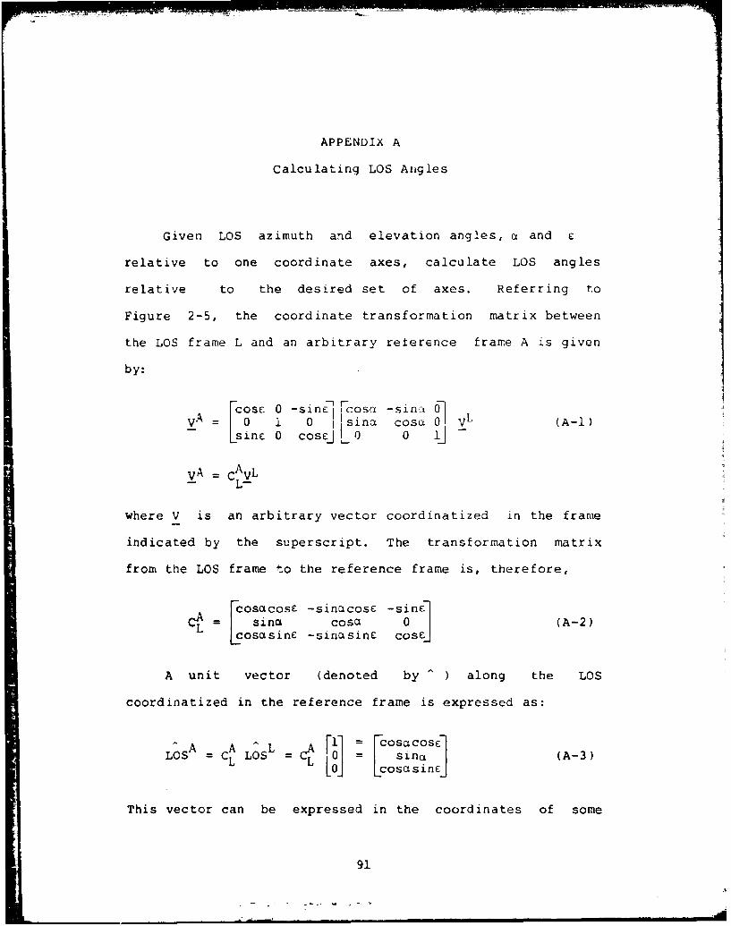
APPENDIX A

Calculating LOS Angles

Given LOS azimuth and elevation angles, a and ;

relative to one coordinate axes, calculate LOS angles

relative to the desired set of axes. Referring to

Figure 2-5, the coordinate transformation matrix between

the LOS frame L and an arbitrary reterence frame A is given

by:

cose 0 -sin 27 F-cosOi -sin-t 02VA = 1 0 ]sina cosa 0 V_ (A-1)

- sin cos0 L 0 0 -j

L VL

where V is an arbitrary vector coordinatized in the frame

indicated by the superscript. The transformation matrix

from the LOS frame to the reference frame is, therefore,

Fcosacose -sinacosE -sin:]

sina cosa 0 (A-2)L cosctsine -sinasine cose]

A unit vector (denoted by ^ ) along the LOS

coordinatized in the reference frame is expressed as:

LOS - C L LOS L 0 sins (A-3)

This vector can be expressed in the coordinates of some

91

other reference frame B by the Euler transformation betwcen

the frames, such as given in eq. (1). Defining tie

coordinate transformation between frames A and B as:

C11 C,2 C,)

vB = cvA C C VA (A-4)-- A-- ; a _IC3 C 32 C 3 3

The unit vector LOSA is coordinatized in the B frame by

SLOSB- x I C 13 Fco sc3ooS

O LOS C3j osasinc

I= C•c ÷C s +Ccs£I (A-5)

3 1 COC + C zSO + C 3CCSEý

using the abbreviations "c" for "cos" and "s" for "sin."

With the components of the unit vector of the LOS

referenced to the desired frame B defined by eq. (A-5), the

azimuth and elevation angles of the LOS relative to the

B-frame axes are given by:

-1 tan- [ LOSvBj (A-6)

e" ='tan- (LOSxLoB),OSzB ] sin'[ OS]

[(LS XB)2 (LOSB)21 j I

92

APPENDIX B

FilLer Measurement Matrix

This appendix covers tile development of the njjeSUremCeIUt

matrix i[t ;\(t.-)] for the filter update.

As given in Chapter , t x t.t)] is defined as:

H.Lt ;Ž(t i )-= mx(ti) ,t H-_ 7 (37)

- - - ?x x= _~t )

and, from eq. (44), hLx tL ) ,tJ is:

C +- +C x-7

V 1 tan-l +C x +Cxi j

tan-'I[•

ic x C x C x )-+C X +-C x5)

tan X

h*x(ti) t ij tan X5

x 1x -x 2x

2 2x I x 3x

(x 1 Ž+x 3 )x 6 -(XŽ+X 3 X-9XS j I

(x +1 2+X 3 2)1, (x 2+ x 3 x 5 )

(B-i)

93

S. . .. -- -.

where, again, the CoeC f iuieiits C tlhrough C arc the

elements of the transformation matrix from the missile frame

to the body frame defined in eq. (1) and described on page le

The partial derivatives as defined by eq. (37) yield a

6 x ) HfLt i ; Ktti )] matrix for the b-state, b-measurement

filter model of this thesis. An example of the evaluation

of Hit-Ji ] ib (chioosing element Ht arbitrarily)

H3 3 X x a

x 2x

X3 3

xl

1 3(

Following this procedure, all 36 elements of Hti;A(ti )J

are given as follows:

Defining:

x, = C x +C 2 x3 +C3 x (B-2)

y = C 4 x+C 5x 3 +C x. (B-3)

Z' = C x IC x 3+Cx (B-4)

H = _i&__• (B-S)

94

it = 0 (B-6

C x<-Cy "

H13 - x 2+ (B-7)

H =0 (B-4)

C6 x -C3 y (B-9)

H1- =0 (B-10)

H 2 = 7 (X 12+y 12) • ( C x.+y + z ). ) B -I I1

-1 = 0 (B-12)

C8 (x +y -: (Cx+C y)3h'23 Z(. -1r z ( . +.- + + •- 3)

H2• 4 0 (B-- 14

H CC9 (x 2 +y 2 ) Z(Cx +C',y (B-15)2a 5 (X , +y .z+(X .a+y 2 +z Z B 1

H2 6 = 0 (B-16)

-xH - (B-17)

31 1 2 x

H =0 (B0S)

xH33 2 2 (B-19)

x + XS3

H 3 0 (B-20)

95

I I "- M O M

13 = 0 (B-21)

I1 = 0 (B-22)

H4 1 1 -x 1x 5 (B-23)(x +x 2) (x '*x 2 +x

3 3 5

4= (B -24)

-X3 XH- -=- (B-25)1j(X 2 Z+X 2)•. X 3 1 3 + 5

H = 0 (B-26)

(x L 4 .,., 2_)=% 3 - 2 7)

46 = 0 (B-28)

H = 2x x x +( 32_ -X1 2 )X4( -921 x x x 2x3 2 )H5 = (1 2 2 (B-29)

-xH23 2 (B-30)

52 X +X1 3

(x 32 -x 1 2 )x - 2xIx 3x

[is3 (x I.:.x 22 (B-31)

1 3

H = 0 (B-33)55.

H56 ,0 (B-34)

96

"2 X 2+ -ý2+x2÷ ]

H =

SI2 + 2X'3 (x 2+X32+X 5-Z)2

(B-3S)

[ = [x 1 X2 +x3 x4)X- (X1 + )x -

-x x

1 (B -36 )6" (x I+x 3 2)(x 1 x 2++) (B-2)2 2 2) ~X% +X,2. -

(Y+X 2 +x 52 ) +(2x -X'X 5s+x 3 [-] +-- 5 +x [

a3 5 2 . 23 2 3 X X

1 J2x X ixsz)3 (B-37)

-x xH6 (x 2 +x 3 Z)½(x 5+x 2 2 (B-38)

x = 1 +X + 3 12+X 1 +X39

H 6 5 2X - 1 (B-39)(x 2 +X3

2)½(xl +X3 +X5 2 )

(x1 + 23½H = (B-40'66 2 2 2

In summary, this appendix is the development of the

measurement matrix HI[ti;_(ti )] for the filter update. The

elements of the H matrix listed as eqs. (B-S) through (B-40)

are evaluated at ti with _(ti') each filter update cycle.

The matrix iI thus calculated is then uses to calculate the

filter gain K(t.) and to update P(ti) as shown in eqs. (36)

and (39).

97

.. S

APPENDIX C

Filter Tuning Plots

98

Cl

II

/ 0 0

I "4

I C3

0o, 002010,31 0*0 0 Lvo- OC 0*00-CIJ) ýIO3 NOI.LISOcF-X

99

7O

0

00

I La

100

o 7-

7--

CdX-1

-C3

U,.

0 06

(),Dot 0.; 010 o*9-____ (

101

9

144

C22

U3

0oza o's C01 OST0 0-s- 0-01- o.sl- 00-oz

102

/ -4

9 P.

103-

C4

Lii

1044

C3.

1050

90

0)

3C

ft.CC

C2 -)

0)o~c asGT o-61 o s 0o Olf- 00T- olst- olor- z

(03S/ J) ý0&12 ý11'0'13 -X t

106

9I

r4J

V)

to)

107

r

0

-4('Is C"C)2

o

ct*)

I I ic

I j 2C)

-4

I 4 II-.

1 0

o� asi oot os7�o�- 00

os 00 001-

108

X 7,

I9

19)

9C

LaL

0O0m 00S1 0.0,0 0o1's 0*0 oots- 000T- o~csl-otQo-

109

9 -

13-

110~

C3N

U4U

Lr0

N080 NOIISOc'J

In

~ C!

4-J

BIC D*' I *1 a* O

112:

Ea

40

C;III

T--

ME OST O= oos 0 0. s- 0 001 O'GI-OO LiUJ) IMO OIII~ciV

113;

19~

CCD

I3t/ U;'-

/r

/C

'11

InI

LO

C2

II

115-

r4

CD

9

11-.

3--4

-0

d r4

cl4

C3

(Na

-eaj

W))

9d -4

UJ)Cr -U3NIIO-

118Z

444

clI

r-I

UI3012A)

Lrn

Cd-

O-9.

Uco

0 waOl col oo 'c- 001 *S-lg-

12G1

Ql

rýJ

tJ)

121

CD

Lfn

m4/<$:

0*01alo *01- olCz

(33S/LJ) -1&3XIO'3

122)

cif

F-4

C,4

0.0' '0 - 4 o C6 C)-0- -n ~o:

1233

I.l 1;ý0

I ~Lf

C)

op-I1m)

VC

-4

00

r4)

0*09 O.s 001 O.s 0.0 0-s- 0o1I- o-sl- Ou-M--

124

9

C!4

C -l-

VV

LLi

C214 c

D~coz *0 0*=11" O IIOZ

-C!

Lfl

[(Nj

C3)

)U

Cdl

C2 to

'-4

0 ore.WN83 X10013A-

126

00

C5CEd)

C!C

14

9 (U

Eg

9/

1272

--

9

91

CC

II 01

I oroI . 00 oi 10- 041 -. --

I3S/J a)3XIO'3-

128,

Cý

IJ QM OLIO-

1129

CC

90

0

0

C2)

9C JC

0. 0

o~e it C-ý O*S 010 019 0*0- CO- loz

I130

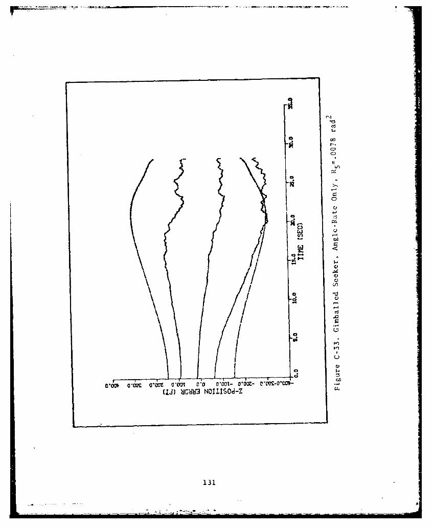
-~ -.-.-.--- ~- - - -0

Cý

'IC-)

L.1

Yo I

( Ci

L)

o, oo* a,= ~v Qo . 0-001- o.0oz- cL0-O-(Ii) 1JC3 NOILISOd-Z L

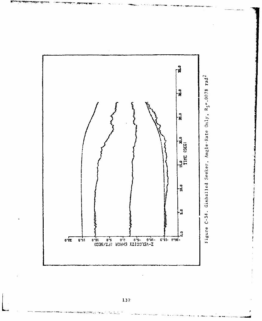
111

---

0.

13J

Lt2

40

"~L

IC7

ciC

a c~z0 0 ~ ooz o .cv- -009

(1j) 108j Nollsoj/

133

Lfl

II

LOl

'-4

C:C)

C.3 I

z )Ii 1-

ifi

~09 wT 0

Clue o*sl 0*x O's oo0 a ocv- o~st- ooce-(03S/Id) 808ý3 XJ.100'13A-Z L.

134

APPENDIX D

Plots for the Results

3

135

",4

aa

-CID0

ELI

EI)

/ Cd/ O'-'

a 70i odv-wc~ 0 0.01- --m O-N-000/(1-9 Wrj olloc

136

C!

C-)L63~

I LA

no

I C3

0.o i 06 S 00 o-. 001 DIM o10S/I 800II03 -

I 137

__ - - �.-w- - - -. � -� -�

-l

0

o

HLa(0

'A

Li.2E -�A �..5-

(I I() K

Q*� o.os1 o*ci�� �as 0 C 0 c� �ov�- os;-oo�z-

JI4

13�

:5-

S.

Win

4-)

.00

0c l oz 01o 0.9 00 0!9- 0101- 0*1- Gooz-

139

C&I

0

A '

0100 aO*N ooo0 oc c OTS- WW~I- aoMI-olov-

140

$-4( I' I"

11

4-)[---4

0)

-4

-4

00

0~~~L -6Z COt 00oý

2 -4

142*

uI

V

V)

4-4

Li

41)

I -n

a lt csT ,01 a's 0. 0-- 001- O~i- 0ciC03S/I2 oID110'3-

140

L'1r-

'04-1

U

f,QELIX-,

'-4

'-4

--4

* C

0

LA /

oo4x oo6s1 0aixu OTs 0*0 00os- 0.(6t- oo-Sl-o-aov-(JJ) KMO3 NOIIASOJ-ý

144

,--44-J

EL

,.C

r-0

o -

CD

Cd -

1454

oo

"0

00

00

.-4I

145

"-4 -*-=- i

4-4

ELI

to -

C3)

Do.0 O0 st 0*001 0*os 010 a0s amx os-o-Uj~) NUOrn NOIIISOCI-Z

146

4.J

Ln.

r-4

-C;~

C&2(n

0-

-4

147

4-)

$-4

U4-

C3

I 0

(IJ) ý183NOL.LISOA-X

148

r� �

C

U

o -�

44

a

44

a

C�)

S -4-4

2: 44

U)

J II aI I

44I 0

I --II I__I I

1'*�*��� r-T- r u -vO*� o.s� o.tn os oo o*s- ooi- o�- aol- I

149

U

a)

C2C

C3

U;4

LIrr f C;

ouz ~ ~ ~ ~ ~ ~ 1 0,- *0 ls 00 Oc- Odl

50 -

aa

4J

1W

-o

I

CA

o 0 L

15 -

C)

00

0

)C

aa

151

9U

4-J

(~23

La

00

vc~ O.61 c~ 0* oos- 0*01- *0s-oloz*IJ MI-NOISD

'-Ii

152)

9IF-4

00

cj.

DIM) OIS *1 09OS *0- DS-Um

ý0'88 1110'13A-

1530

494

S.4

-4

9 to

154.

0V)

C3'7W

to

u03/I) 0'-4-IO93-

1554

-94

4-J

-o3

W Z

CJ CU

5 156

C!.

C3

Laco

U3 4

-4

C2C

0 *z ost 0*0 as 0J 0-- 001 0-1-0-m -

157

0c

aa

.0

f-D

CD

ooe *Os 0*01 DOS *0 Oos-0*00 ds-o- oi-UJI NU NCILI-IJ'

1584

9U

C)

9'19 4-)

CC!3

4-14

s-4

CL)

Inn

C)4

ot O-sl 0-ax a's gg 0 .s- o01- O'SI- 0 cz-

159

VITA

Andrew C. Weston was born on 14 August 1959 in

Chattanooga, Tennessee. He graduated from high school in

Barnwell, South Carolina in 1977 and attended The Citadel,

Charleston, South Carolina, from which he received the

degree of Bachelor of Science in Electrical Engineering in

May 1981. Upon graduation he received his commission and

entered the School of Engineering, Air Force Institute of

Technology in June 1981. His next assignment is with the

Applications Branch of the Avionics Laboratory,

Wright-Patterson Air Force Base. He is a member of IEEE

and Tau Beta Pi.

Permanent address: 107 Woodlawn Avenue

Union, S. Carolina 29379

160

7=

un•lassifitdSECURITY CLASSIFICATION OF ý-,S PAGE (Wh-n Date Entered)

PAGE IREAD INSTIRUCTIGN ZREPORT DOCUMENTATION PAGE BEFORE COMPLETI__ F__'__,

1. REPORT NUMBER '2 Go i *. Nk. 3 RECIPIENT'S CATALOG NIUM9c

AFIT/GE/EE/82D-70 6 1VI"4. TITLE (and Subttfle) S. TYPE OF REPORT & PERIOD C-, "•-

DUAL-SEEKER MEASUREMENT PROCESSING MS Thesis

FOR TACTICAL MISSILE GUIDANCE 6. PERFORMING ORG. REPORT NumaER

7. AUTHOA(m) 8. CONTRACT OR GRANT NUMBER.S

Andrew C. Weston2Lt USAF

0. PERFORMING ORGANIZATION NAME AND ADDRESS I0. PROGRAM ELEMENT. PROJEZ- -- ,-K

Air Force Institute of Technology AREA & WORK UNIT NUMBERS

(AFIT-EN)Wright-Patterson AFB, Ohio 45433

1I. CONTROLLING OFFICE NAME AND ADDRESS 12. REPORT DATE

Terminal Guidance Group, Armament December 1982Laboratory 13. NUMGER OF PAGES

Eglin AFB, Florida 32542 17214. MONITORING AGENCY NAME & AODRESSeif dlfferenr from Concrollinc Office) IS. SECURITY CLASS. (of thll. rep-r*

Unclassified

IS&, OECLASSIFICATI:N OOWNsR, \A

SCHEDULE

16. OISTRIOlUTION STATEMENT (of this Reporf)

Approved for public release; distribution unlimited

I'7. DISTRIBUTION STATEMENT (of the abstract entered In Block 20, it different from Re.ort)

18. SUPPLEMENTARY NOTES ,IAN. Az 1 FJ-1 .

W9. KEY WORDS (Continue on reveree side If neesaeery ad idantf y by block number)

Air-to-Ground Tracking Gimballed SeekerDual-Seeker Kalman FilterStrapdown Seeker Air-to-Ground Missile

20. ABSTRACT (Conltnue on reverse aide it necessIry and Identlfy by block number)

The available measurements from a strapdown seeker anda gimballed seeker onboard an air-to-ground anti-radiationmissile are analyzed through an extended Kalman filtersimulation. Detailed models of both seekers are developed.

Only angular measurements are assumed available from theseekers: angle measurements from the strapdown seeker and

FORM

DD JAN 7 1473 EOITION o0 1 NCV S5 IS OeSOLETElL unClassifIC F GdSECURITY CLASSIFICATION OF THIS IPAGE (I

47•er Date Enr.e,e,

_ , 1c a_... s I ed

20. angle and angle-rate measurements from the gimballedseeker. A 6-state extended Kalman filter model is used toestimate the ground target's position and relative velocityusing the seekers' measurements. Four measurement policiesare compared to analyze use of the gimballed seeker earlyin tile missile flight and loss of the strapdown seaker inmidf light.

The results revealed an observability problem in onechannel of the filter, that along the range vector.Analyses were made only by comparisons of per'2ormance inthe other two channels. The comparisons showedinsignificant degradation to filter performance throughloss of the strapdown seeker at midflight, and substantialbenefit from use of the gimballed seeker as early aspos:3ible in the flight.

uviclassif ied

st~ijQ. y L V # C 1!J- P G~~he V 's ~efI