SANDIA REPORT SAND2010-6678 Unlimited Release Printed September 2010

LDRD 149045 Final Report Distinguishing Documents Scott A. Mitchell Prepared by Sandia National Laboratories Albuquerque, New Mexico 87185 and Livermore, California 94550 Sandia National Laboratories is a multi-program laboratory managed and operated by Sandia Corporation, a wholly owned subsidiary of Lockheed Martin Corporation, for the U.S. Department of Energy’s National Nuclear Security Administration under contract DE-AC04-94AL85000. Approved for public release; further dissemination unlimited.

Issued by Sandia National Laboratories, operated for the United States Department of Energy by Sandia Corporation. NOTICE: This report was prepared as an account of work sponsored by an agency of the United States Government. Neither the United States Government, nor any agency thereof, nor any of their employees, nor any of their contractors, subcontractors, or their employees, make any warranty, express or implied, or assume any legal liability or responsibility for the accuracy, completeness, or usefulness of any information, apparatus, product, or process disclosed, or represent that its use would not infringe privately owned rights. Reference herein to any specific commercial product, process, or service by trade name, trademark, manufacturer, or otherwise, does not necessarily constitute or imply its endorsement, recommendation, or favoring by the United States Government, any agency thereof, or any of their contractors or subcontractors. The views and opinions expressed herein do not necessarily state or reflect those of the United States Government, any agency thereof, or any of their contractors. Printed in the United States of America. This report has been reproduced directly from the best available copy. Available to DOE and DOE contractors from U.S. Department of Energy Office of Scientific and Technical Information P.O. Box 62 Oak Ridge, TN 37831 Telephone: (865) 576-8401 Facsimile: (865) 576-5728 E-Mail: reports@adonis.osti.gov Online ordering: http://www.osti.gov/bridge Available to the public from U.S. Department of Commerce National Technical Information Service 5285 Port Royal Rd. Springfield, VA 22161 Telephone: (800) 553-6847 Facsimile: (703) 605-6900 E-Mail: orders@ntis.fedworld.gov Online order: http://www.ntis.gov/help/ordermethods.asp?loc=7-4-0#online

2

SAND2010-6678 Unlimited Release

Printed September 2010

LDRD 149045 FINAL REPORT DISTINGUISHING DOCUMENTS

Scott A. Mitchell

Computation, Computers, Information and Mathematics P.O. Box 5800, MS1316

Sandia National Laboratories Albuquerque, NM 87185

ABSTRACT This LDRD 149045 final report describes work that Sandians Scott A. Mitchell, Randall

Laviolette, Shawn Martin, Warren Davis, Cindy Philips and Danny Dunlavy performed in 2010. Prof. Afra Zomorodian provided insight. This was a small late-start LDRD. Several other ongoing efforts were leveraged, including the Networks Grand Challenge LDRD, and the

Computational Topology CSRF project, and the some of the leveraged work is described here.

We proposed a sentence mining technique that exploited both the distribution and the order of parts-of-speech (POS) in sentences in English language documents. The ultimate goal was to be able to discover “call-to-action” framing documents hidden within a corpus of mostly expository

documents, even if the documents were all on the same topic and used the same vocabulary. Using POS was novel. We also took a novel approach to analyzing POS. We used the hypothesis that English follows a dynamical system and the POS are trajectories from one state to another. We analyzed the sequences of POS using support vector machines and the cycles of POS using

computational homology. We discovered that the POS were a very weak signal and did not support our hypothesis well. Our original goal appeared to be unobtainable with our original

approach.

We turned our attention to study an aspect of a more traditional approach to distinguishing documents. Latent Dirichlet Allocation (LDA) turns documents into bags-of-words then into

mixture-model points. A distance function is used to cluster groups of points to discover relatedness between documents. We performed a geometric and algebraic analysis of the most

popular distance functions and made some significant and surprising discoveries, described in a separate technical report.[9]

3

4

INTRODUCTION The goal of the work was to distinguish faming (call to action) documents from expository (explanatory, action-neutral) documents. Most work in the area of text analysis depends on modeling the words in documents: e.g. “recent”, “car”, “anger”, “oil” and 20,000 others. This works well in discovering topics, but less well for distinguishing between framing vs. expository. Instead our idea was to focus on the parts-of-speech (POS) in English sentences: e.g. “comparative-adjective”, “conjunction”, “plural-noun”; 36 in all. Additionally, in contrast to the bag-of-words model, we chose to focus on POS order. Note the choice of English is important here, because in an inflective language such as Latin the word ending (form) defines its meaning, and order does not change the meaning. English is mostly syntactic and only mildly inflective. It is actually losing inflection over time (as are many other languages). For example, “Drive Slow" is now accepted in place of the more inflected “Drive Slowly"; “Slowly Drive", though awkward, would convey the same meaning. But “Slow Drive" would be ambiguous if not completely meaningless to most people. In particular, our multi-part hypothesis was that (1) the order of the POS would distinguish document types, that (2) the POS followed a dynamical system, and that (3) the tools of computational homology could discover the trajectories (cycles) of this dynamical system through the observed POS and (4) this would reveal something about the underlying “states” that differed in framing vs. expository writing. In retrospect our multiple hypotheses were overly ambitious. We discovered that POS are a very weak signal. Using support vector machines (SVM) classification, we showed that short sequences (3 or 4 long) of POS from actual sentences were distinguishable from random orderings of POS, even when the POS came from the same distribution. But the longer sequences that would be necessary to get any more nuanced meaning were not distinguishable. Using topology, there are too many chance repetitions of common POS that produce cycles, which obscured any meaningful cycles. Perhaps English sentences are reflective of a dynamical system, as the beginning of sentences, before and after parenthetical remarks, etc., could be considered as states. Discovering states from observed trajectories is difficult; in our case it is even more difficult because the cycles in POS appear to be very imperfect evidence of trajectories between states. Different trajectories might heavily re-use POS. Various graph models of POS were constructed. We computed the homology of these graphs using the computational homology package JPlex[11]. We developed measures based on the Jaccard index for comparing the homologies of different sentences. We experimented with real-world datasets, attempting to distinguish Netflix movie reviews from groundwater journal abstracts. After we concluded that real-world data did not support our original hypothesis and approach, we changed tack and began to study a more standard text analysis approach. Documents are considered bags-of-words, where the order of words is ignored, and the POS are ignored. Latent Dirichlet Allocation (LDA) builds mixture models of topics in word-space and of documents in topics-pace. Points of the mixture models are then clustered using a distance function. We studied the popular distance functions for this problem, using basic geometry and algebra. We

5

discovered some fascinating relationships between these common functions, which were surprising to the people who are using these functions all the time. We summarized our findings in a 24 page technical report, “Geometric comparison of popular mixture-model distances”[9]. We wrote a proposal for Sandia’s Cyber LDRD IA to further develop this analysis for cybersecurity applications. Proposal Here we reproduce our original proposal as a description of the problem and what motivated our work. Readers may skip ahead to “Homological Approach”. Project title: Distinguishing documents by part-of-speech dynamics Principal Investigator’s name: Scott Mitchell Research staff: Scott Mitchell, Randall Laviolette, Danny Dunlavy. Budget requested: $45k Project Manager’s name: David Rogers Proposal abstract: We propose a sentence mining technique that exploits both the distribution and the order of parts-of-speech (POS, as define by the Penn Treebank) in sentences in English language documents. The research is focused on discovering meaningful sentence dynamics (grammar) signatures. If successful, it would be possible to discover “call-to-action” framing documents hidden within a corpus of mostly expository documents, even if the documents were all on the same topic and used the same vocabulary. This distinguishes the proposed work from ongoing activities in topic identification, which analyzes the bag of words in documents using linear algebra. While the rules of grammar are specified a priori by linguists, this would be the first known computational approach to discovering and characterizing actual, observed English grammar. Distinguishing framing vs. expository documents within unknown topics is the most important problem of this type, but this late-start would start with an easier problem with readily available data. We seek to distinguish opinion vs. exposition, in particular distinguishing Netflix “positive” and “negative” movie reviews from abstracts from a groundwater science journal, without exploiting topic and word differences. Our preliminary work shows that the cosine similarity of the subsequences of POS is able to distinguish between abstracts and Netflix; and also (1) actual sentences and (2) the same sentences reversed and (3) the same sentences with their POS randomly permuted. It appears that sub-sequence lengths between 2 and 5, especially 3, is a better differentiator than the just the frequency of POS (i.e. sub-sequence length 1).

6

Figure 1. Cosine similarity for subsequence length 1,2,3,4,5, between 100 scientific abstract sentences, the same sentences backwards, and the same sentences randomly permuted.

2 3

Figure 2. Cosine similarity for subsequence length 2 and 3, between 100 scientific abstract sentences and 100 “negative” movie reviews and 100 “positive” movie reviews. Description of the work proposed: We suspect that English follows a dynamical system with hidden (not directly observable) rules. Beyond cosine similarity, the fixed-points, the POS that are repeated, and the loops of POS that appear between the fixed-points, were analyzed using persistent homology (JPlex) over some filtered simplicial complexes (adding simplices for consecutive POS between fixed points). Homology appears to provide some differentiating signal. However, we have not yet discovered the right structures and measures in order to both differentiate and cluster the documents. The proposed work is to discover these, and demonstrate them in an end-to-end computational system, for our restricted datasets and types. We will explore different subsequences, especially those between fixed points. We seek to augment persistent homology with measures that consider tags on the data to overcome the problem of the skewed distribution of POS. Also, fixed-points joined by long loops appear to be an artifact of the distribution and should be ignored. How the work supports the DOE national security mission: This work supports text analysis, which is important for non-proliferation, cyber-security and other data-centric security missions. This work could eventually lead to finding unknown social movements within unknown topics, for the above missions. Eventually we may be able to distinguish: 1. Fluent vs. non-fluent English 2. Machine vs. human generated 3. Opinion vs. narrative, exposition, or enumeration 4. Framing vs. narrative, exposition, or enumeration 5. Framing vs. Opinion Work by Laviolette and Dunlavy on the Network Grand Challenge LDRD and another LDRD provides additional motivation. That project was focused on developing a way to generate surrogate documents. These are synthetic (machine generated) bags-of-words that fall into the same category as a given set of training documents. They are generated using the frequency with which words appear in the training set (the stateless Bernoulli model). But beyond that, are also generated based on the probability that a word starts a sentences, and the conditional probability

7

of what word follows another (the Markov model, where the next state depends on prior state but only the one-prior state). Our proposal would extend this in the sense that we would be considering longer POS sequences, longer state history. Homological Approach Here we describe the motivation and background of homology in more detail, and how we applied this approach to POS sentence dynamics. Maturity of Homology for Research and Applications Algebraic homology is an old math field, with new (<10 year old) computational tools. Its appeal is that it can discover global information from local structure. Sandia has a large investment in a variety of other tools for the general area of discrete structure discovery and analysis. Homology provides complementary and unique information beyond these. These other tools include graph algorithms, statistics, and tensors. Homology overlaps with the graph properties of connectedness and spanning trees. Homology can represent higher dimensional objects than graphs, simplices of arbitrary dimension, whereas graphs are limited to 0-dimensional vertices and 1-dimensional edges. On the other hand, graph theory can do some things homology can not, such as model directed graphs, attributes on edges and vertices, and can more easily model the dynamics of graphs adding and removing vertices and edges. Homology can model the dynamics of adding simplices, but homological tools for removing them are limited to zigzag complexes and are more difficult. Homology has ties to electromagnetic PDE solutions, in particular the kernel of operators related to the phenomena of orthogonality between electric and magnetic fields and eddy currents[4]. Homology is related to Morse Theory, and the Sandia-CA combustion group (Pebay, Bennett, et al.) has an ongoing project with Sandia-NM’s visualization department (Shepherd et al.) on using a topological tool called Reeb graphs together with statistics to study ignition and extinguishment in combustion simulations. Homology has ties to cryptography, in that the Smith-Normal Form over finite field algebra can be used to solve problems in both.

• Visualization via Morse Theory for turbulent mixing (left) [6] and manufactured object characterization. Prof. Pascucci with Sandians Bennett, Thompson, Mascarenhas, Grout, and Chen.

Homology is computed in one of two ways. The first way is linear algebra over finite fields, like Gaussian elimination using exact arithmetic. We had hopes to demonstrate the effectiveness of Trilinos[5] for discrete math applications. The second way is based on discrete algorithms over graphs, a matching problem between structures of different dimensions, over a non-bi-partite

8

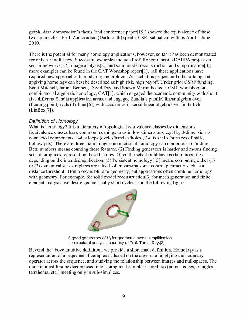
graph. Afra Zomorodian’s thesis (and conference paper[15]) showed the equivalence of these two approaches. Prof. Zomorodian (Dartmouth) spent a CSRI sabbatical with us April – June 2010. There is the potential for many homology applications, however, so far it has been demonstrated for only a handful few. Successful examples include Prof. Robert Ghrist’s DARPA project on sensor networks[12], image analysis[2], and solid model reconstruction and simplification[3]; more examples can be found in the CAT Workshop report[1]. All these applications have required new approaches to modeling the problem. As such, this project and other attempts at applying homology can best be described as high risk, high payoff. Under prior CSRF funding, Scott Mitchell, Janine Bennett, David Day, and Shawn Martin hosted a CSRI workshop on combinatorial algebraic homology, CAT[1], which engaged the academic community with about five different Sandia application areas, and engaged Sandia’s parallel linear algebra over (floating point) reals (Trilinos[5]) with academics in serial linear algebra over finite fields (LinBox[7]). Definition of Homology What is homology? It is a hierarchy of topological equivalence classes by dimensions. Equivalence classes have common meanings to us in low dimensions, e.g. H0, 0-dimension is connected components, 1-d is loops (cycles/handles/holes), 2-d is shells (surfaces of balls, hollow pits). There are three main things computational homology can compute. (1) Finding Betti numbers means counting these features. (2) Finding generators is harder and means finding sets of simplices representing these features. Often the sets should have certain properties depending on the intended application. (3) Persistent homology[15] means computing either (1) or (2) dynamically as simplices are added, often varying some control parameter such as a distance threshold. Homology is blind to geometry, but applications often combine homology with geometry. For example, for solid model reconstruction[3] for mesh generation and finite element analysis, we desire geometrically short cycles as in the following figure:

Beyond the above intuitive definition, we provide a short math definition. Homology is a representation of a sequence of complexes, based on the algebra of applying the boundary operator across the sequence, and studying the relationship between images and null-spaces. The domain must first be decomposed into a simplicial complex: simplices (points, edges, triangles, tetrahedra, etc.) meeting only in sub-simplices.

graphic from Prof. Dey

6 good generators of H1 for geometric model simplification for structural analysis, courtesy of Prof. Tamal Dey.[3]

9

boundary operator

+-

graphic and equations from Prof. Vegter The boundary of the boundary is null, due to sign (or “orientation” or “coefficients”). Thus we may define a sequence of boundary operators on a sequence of algebraic spaces: in the following figure Ck is the space of simplices of dimension k in the complex, Zk is the kernel of the kth boundary operator, and Bk is the image of the prior (k-1th) boundary operator

If Bk = Zk, then this is called an exact sequence. Homology studies how much this differs from being exact. That is, there are often objects in the kernel that are not the boundary of higher-dimensional objects. These objects are exactly the interesting features we are looking for. For example, each of the two loops in the following figure of a torus are in the kernel Z1 since they have null boundary, because they are closed. However, they are not in the boundary image B1 because neither one bounds a set of quadrilaterals.

not-quite exact sequence

kernel graphic from Prof. Zomorodian

Formally, these objects are generators (basis elements for) the quotient group Hi = kernel(∂i)/image(∂i+1). These quotient groups are the “homology” groups, indexed by dimension i. The number of these generators is the rank of the group, the Betti numbers.

10

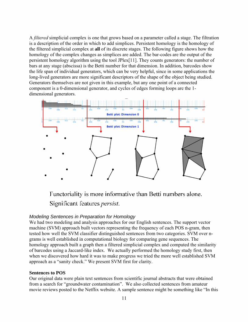
A filtered simplicial complex is one that grows based on a parameter called a stage. The filtration is a description of the order in which to add simplices. Persistent homology is the homology of the filtered simplicial complex at all of its discrete stages. The following figure shows how the homology of the complex changes as simplices are added. The bar-codes are the output of the persistent homology algorithm using the tool JPlex[11]. They counts generators: the number of bars at any stage (abscissa) is the Betti number for that dimension. In addition, barcodes show the life span of individual generators, which can be very helpful, since in some applications the long-lived generators are more significant descriptors of the shape of the object being studied. Generators themselves are not given in this example, but any one point of a connected component is a 0-dimensional generator, and cycles of edges forming loops are the 1-dimensional generators.

Modeling Sentences in Preparation for Homology We had two modeling and analysis approaches for our English sentences. The support vector machine (SVM) approach built vectors representing the frequency of each POS n-gram, then tested how well the SVM classifier distinguished sentences from two categories. SVM over n-grams is well established in computational biology for comparing gene sequences. The homology approach built a graph then a filtered simplicial complex and computed the similarity of barcodes using a Jaccard-like index. We actually performed the homology study first, then when we discovered how hard it was to make progress we tried the more well established SVM approach as a “sanity check.” We present SVM first for clarity. Sentences to POS Our original data were plain text sentences from scientific journal abstracts that were obtained from a search for “groundwater contamination”. We also collected sentences from amateur movie reviews posted to the Netflix website. A sample sentence might be something like “In this

11

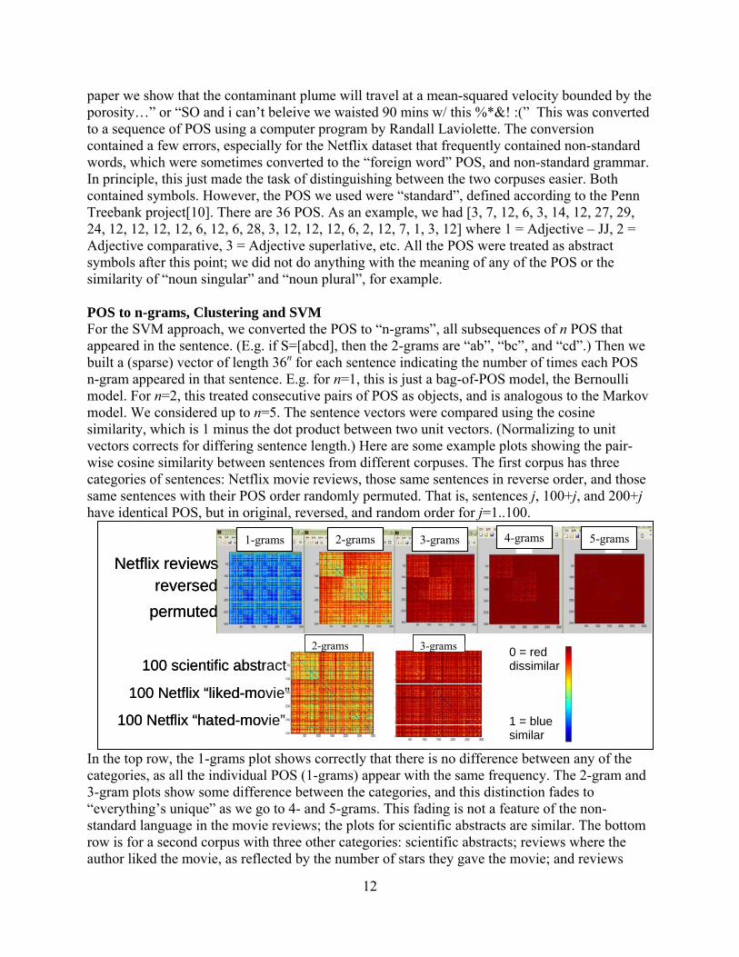
paper we show that the contaminant plume will travel at a mean-squared velocity bounded by the porosity…” or “SO and i can’t beleive we waisted 90 mins w/ this %*&! :(” This was converted to a sequence of POS using a computer program by Randall Laviolette. The conversion contained a few errors, especially for the Netflix dataset that frequently contained non-standard words, which were sometimes converted to the “foreign word” POS, and non-standard grammar. In principle, this just made the task of distinguishing between the two corpuses easier. Both contained symbols. However, the POS we used were “standard”, defined according to the Penn Treebank project[10]. There are 36 POS. As an example, we had [3, 7, 12, 6, 3, 14, 12, 27, 29, 24, 12, 12, 12, 12, 6, 12, 6, 28, 3, 12, 12, 12, 6, 2, 12, 7, 1, 3, 12] where 1 = Adjective – JJ, 2 = Adjective comparative, 3 = Adjective superlative, etc. All the POS were treated as abstract symbols after this point; we did not do anything with the meaning of any of the POS or the similarity of “noun singular” and “noun plural”, for example. POS to n-grams, Clustering and SVM For the SVM approach, we converted the POS to “n-grams”, all subsequences of n POS that appeared in the sentence. (E.g. if S=[abcd], then the 2-grams are “ab”, “bc”, and “cd”.) Then we built a (sparse) vector of length 36n for each sentence indicating the number of times each POS n-gram appeared in that sentence. E.g. for n=1, this is just a bag-of-POS model, the Bernoulli model. For n=2, this treated consecutive pairs of POS as objects, and is analogous to the Markov model. We considered up to n=5. The sentence vectors were compared using the cosine similarity, which is 1 minus the dot product between two unit vectors. (Normalizing to unit vectors corrects for differing sentence length.) Here are some example plots showing the pair-wise cosine similarity between sentences from different corpuses. The first corpus has three categories of sentences: Netflix movie reviews, those same sentences in reverse order, and those same sentences with their POS order randomly permuted. That is, sentences j, 100+j, and 200+j have identical POS, but in original, reversed, and random order for j=1..100.

In the top row, the 1-grams plot shows correctly that there is no difference between any of the categories, as all the individual POS (1-grams) appear with the same frequency. The 2-gram and 3-gram plots show some difference between the categories, and this distinction fades to “everything’s unique” as we go to 4- and 5-grams. This fading is not a feature of the non-standard language in the movie reviews; the plots for scientific abstracts are similar. The bottom row is for a second corpus with three other categories: scientific abstracts; reviews where the author liked the movie, as reflected by the number of stars they gave the movie; and reviews

Netflix reviewsreversed

permuted

1-grams 2-grams 3-grams 4-grams 5-grams

Netflix reviewsreversed

permuted

1-grams 2-grams 3-grams 4-grams 5-grams

3-grams2-grams

100 Netflix “liked-movie”

100 Netflix “hated-movie”

100 scientific abstract3-grams2-grams

100 Netflix “liked-movie”

100 Netflix “hated-movie”

100 scientific abstract0 = red dissimilar

1 = blue similar

12

where the author hated the movie. Note the scientific abstracts are more like each other than the movie reviews, reflective of adhering to the same writing style. We (Warren Davis) also tried clustering the sentences using a dendrogram (tree) view that paired sentences in sequence, pairing the most similar pair, then the next most similar pair, etc.; see the next figure left. Unfortunately, the tools we had at the time, from an external source, only showed the resulting pairing, not the relative strengths of the pairings, so it was not possible to tell if the original categories (the ground truth) were reproduced. These tools, too, were designed for comparing gene sequences in computational biology. Warren has since undertaken the task of putting a more powerful version of this capability into Sandia’s Titan visualization software[14]. Shawn Martin built a SVM classifier on the n-grams for the second corpus. This showed that the 2- and 3-grams were the most distinguishing, which was consistent with the cosine similarity plots. This was not encouraging for supporting our hypothesis, which relied on long sequences of POS being significant and indicative of trajectories.

Dendrogram greedy pairing

SVM on 100 scientific + movie

POS to Homology Many choices were possible in building a filtered simplicial complex[15], and we (Scott Mitchell, Randall Laviolette) tried several variations, guided by what seemed most likely to find supporting evidence for the hypothesis, if it existed. We first describe a graph model, then how we modified it to be a complex. First, thinking of English sentences as discrete dynamical systems, it was natural to consider POS as vertices (0-cells) and directed edges between consecutive POS in the sentences. We consider a graph for each sentence. This graph will have cycles, indeed our hypothesis was that these cycles were the interesting structure indicating the underlying dynamical system. But we were faced with the question of “How can we represent directed edges?” While one may assign coefficients to simplices in simplicial complexes from any choice of ring, there is no known way of combining these assigned coefficients together with homology calculations, because the

13

boundary operator introduces its own coefficients that are necessary for calculating the kernel, etc. So as a first pass we simply dropped the directedness of the edges, but chose the filtration order reflective of direction. That is, let S be the array of POS in a sentence. At filtration stage 0 we introduced all the vertices for the POS that appeared in the sentence. At filtration stage 1 we introduced the edge (1-cell) between the vertex for the first POS appearing in the sentence (S[1]) and the second POS appearing in the sentence (S[2]), etc. From here we tried several variations, but this initial set-up remained constant. Computing persistent homology on this model would identify the number of unique POS and the number of edge cycles, together with the index into the sentence when loops were first formed. 2-cycles One consequence of dropping the directedness was we had no way to represent 2-cycles, pairs of POS that appeared both forward and backward, as in the 2-cycle between 1 and 2 in the sentence [1 2 3 4 2 1]. So one variation we tried was splitting each vertex in two, say V1 and V1′ for POS 1, with an edge between them at filtration stage 0. For consecutive POS S[i] and S[i+1], if S[i]>S[i+1] we introduced an edge between VS[i] and VS[i+1]. Otherwise we introduced an edge between VS[i]′ and VS[i+1]′. Thus 2-cycles would appear as 1-d homology generators. 1-cycles Also, because simplicial complexes represent simplices, we had no way to represent 1-cycles of the form S=[11]. So a second variation was to split vertices into three, VS, VS′, and VS′′, and two edges VS-VS′ and VS′-VS′′ at filtration stage 0. Then if S[i]=S[i+1], we would introduce the third edge VS-VS′′ completing a cycle of three edges. Thus 1-cycles would appear as 1-d homology generators. The 2-cycle and 1-cycle variations were dropped in the following as a simplification, in order to focus on measuring the features described next. k-cells The hypothesis was that cycles were trajectories, so we wanted a better way to distinguish between cycles than the stage at which they appeared. One measure was the length of the cycles, another was the extent to which cycles interleaved. We modeled this by filling in cycles starting with a filtration index after the last edge was introduced, the length of the sentence, say K. At stage K+2, we added a triangle (2-cell) between S[i],S[i+1],S[i+2] for every i that started a cycle. In general, for filtered simplicial complexes, the notion of starting a cycle is not unique. But for us, with each edge introduced in sequence, when a cycle is formed at stage j, by introducing edge VS[j],VS[j+1], we know that the sentence has structure [S[1], S[2], …. S[i], … S[j], S[j+1], …] where S[i]=S[j+1] for some i. We pick the largest index i<j+1 where S[i]=S[j+1], and now i is one of the indices at which we add a triangle. At stage K+k, we add k-cells S[i],S[i+1],…S[i+k] for all such i. Measures on Barcodes Barcodes represent the lifespan of cycles over filtration stages. Homology has been used to compare images. In that context, the Jaccard index proved useful, so we considered it here as well. The Jaccard index is defined as the following for sets:

14

To apply this to intervals, we convert an interval to the integer stages is covers. This gives us a measure of similarity between two intervals, value 1 if the intervals are identical and 0 if they are disjoint. To turn similarity into a distance, we use 1-J. Also, our data are sets of intervals, one set for each sentence for each homology dimension. Sets for different dimensions are incomparable, and we produced one measure of comparison between 0-dimensional barcodes, and two others for 1-dimensional barcodes. We split the 1-dimensional barcodes into two sets, one set for the stages <K when we were just introducing edges, and one set for afterwards when k-cells were introduced. For the pairs of sets of comparable barcodes for two sentences, we did an optimization, matching one interval from one sentence to one interval from the other sentence, and found the matching that produced the minimum sum of distances (1-Jaccard indices). (Before matching, we first aligned the entire set based on the stage K where triangles were first introduced, to minimize the effect of sentence length.) The matching was performed using the optimization toolbox within Matlab, and no computational difficulties were encountered. Cindy Philips helped with this formulation. One sentence often has more intervals than the other, leaving some intervals unmatched. We tried various schemes to weight these. One option is to apply the Jaccard index with A=interval, and B=empty set, which contributes a value of 1 (Jaccard index being 0). At the other extreme the unmatched barcodes could be ignored. We found that a value between these, increasing with the size of the interval, produced the most meaningful comparisons. In any case, these distances are probably not true metrics, and much analysis could be done to consider their properties and effects. Future Variations Possible variations are to anchor cycles by the POS of their start vertex, e.g. matching nouns to nouns, instead of by their filtration stage. Another variation is to consider something other than individual POS as vertices: POS pairs, or entire cycles in the sentence graph. Results The results were inconclusive. We were not able to come up with models or measures that reproduced the “ground truth” of the known different categories within the corpus. Here we highlight some of the discoveries/challenges. First, the cycles overlapped to a very strong degree, stronger than we imagined. Most 1-cycles were filled in by just 2-cells and 3-cells, indicated by the barcodes terminating at stages K+2 and K+3. This was despite the fact that length 7+ cycles are fairly common. This indicates the presence of sub-cycles, but not necessarily within the sequence defining the long cycle. That is, this indicates the presence of short cycles somewhere in the sentence that use the same POS as the long cycle.

15

The frequencies of POS are not uniform. We have not done enough analysis to claim POS follow a power law distribution, but it is known that the frequency of English words do follow a power law. In any case the POS were highly skewed, with some of them very frequent. We suspect that these frequent POS produced many small cycles that swamped any meaningful signal that longer cycles might produce. Shannon information theory suggests to weight the rare features. It may be helpful to distinguish cycles by index of the POS, rather than by filtration stage. One option for doing this would be to filter (vertices, edges, some combination) by frequency of POS, or re-order or re-number the POS based on frequency, but this loses the sentence order. The measures of 0-barcodes were not very interesting, as these merely indicated the number of unique POS, and when a POS first appeared in the sentence. At best, it measured how many rare POS appeared in long sentences. If one were truly interested in this feature, more direct measurements would be easy and more useful. k-simplices have a lot of sub-simplices, i.e. (k chose j) sub-simplices of dimension j, which is exponential in k. Even an 8-simplex has so many subsimplices that the software we were using, JPlex, would not introduce them for fear of running out of memory. So we had to finesse this issue by only adding subsimplices (of the k-simplex) up to dimension 6, which is O(k6). In the future, perhaps a triangulation of the cycles as closed 2d polygons, O(k), and adding one triangle at each filtration stage would be sufficient. Persistent homology indicated the presence of some high dimensional homology groups, e.g., nontrivial H5. In other applications these have frequently indicated randomness in the data, but we don’t really know what they mean here, if anything. In general, for most applications of homology, it helps to know what the k-dimensional barcodes mean before one starts an application. There are some notable exceptions where it appears that the meaning of structure was discovered after the structure itself: Shawn Martin’s cyclo-octane work[8], some work in the 1980’s on biological species food webs and specialization[13], and perhaps some of the early image analysis work[2]. As mentioned earlier, the cycles of POS may not have much to do with trajectories of the dynamical system we were attempting to characterize. For example, one natural state of the dynamical system is the start of a sentence. A sentence may start and end without producing any cycle of POS, yet the trajectory brought one back to the original state. Further, the dynamical system may not exist at all. The originator of the dynamical system hypothesis, Randall Laviolette, left the project and Sandia in May 2010 for a new career as a program manager at DOE ASCR. Alternate problem, geometric comparison of distance functions over mixture models Given these challenges, we turned our attention to a more traditional text analysis approach for distinguishing documents: LDA to model documents as points in topic-space, and distance functions to cluster those points. We produced some noteworthy research on these distance functions. We do not reproduce that here, but refer the interested reader to the technical report[9].

16

References

1. Janine C. Bennett, David M. Day, and Scott A. Mitchell, “Summary of the CSRI workshop on Combinatorial Algebraic Topology (CAT): software, applications, & algorithms”, Sandia National Laboratories technical report, SAND2009-7777, 2009. http://www.cs.sandia.gov/~samitch/papers/CATreport_finalSAND.pdf

2. Gunnar Carlsson, Tigran Ishkhanov, Vin de Silva and Afra Zomorodian, ”On the local behavior of spaces of natural images”, International Journal of Computer Vision. Volume 76, Number 1, 1-12, DOI: 10.1007/s11263-007-0056-x

3. T. K. Dey, J. Sun, and Y. Wang. “Approximating loops in a shortest homology basis from point data.” Proc. 26th Annu. Sympos. Comput. Geom. (SOCG 2010), pp. 166-175. arXiv:0909.5654v1[cs.CG], 30th September 2009.

4. P. Dłotko and R. Specogna, "Critical analysis of the spanning tree techniques'', SIAM Journal of Numerical Analysis (SINUM), Vol. 48, No. 4, 2010, pp. 1601-1624.

5. Michael Heroux, “The Trilinos Project,” http://trilinos.sandia.gov/ 6. D. Laney, P.-T. Bremer, A. Mascarenhas, P. Miller, and V. Pascucci, “Understanding the

structure of the turbulent mixing layer in hydrodynamic instabilities.” IEEE Transactions on Visualization and Computer Graphics Vol. 12, No. 5, pp. 1053-1060, 2006. Proceedings of IEEE VIS 2006, winner of the best application paper award.

7. LinBox. Project LinBox: Exact computational linear algebra website, linboxuse@googlegroups.com. http://linalg.org.

8. Shawn Martin, Aidan Thompson, Evangelos A. Coutsias, and Jean-Paul Watson, “Topology of cyclo-octane energy landscape”, J. Chem. Phys. 132, 234115 (2010); doi:10.1063/1.3445267

9. Scott A. Mitchell, “Geometric comparison of popular mixture-model distances”, Sandia National Laboratories technical report, SAND2010-6286C, 2010.

10. Beatrice Santorini, “Part of Speech Tagging Guidelines for the Penn Treebank Project”, June 1990. The Penn Treebank Project, http://www.cis.upenn.edu/~treebank/.

11. V. de Silva, D. Banard, P. Lee, and P. Perry, “Plex: Simplicial complexes in MATLAB.” http://comptop.stanford.edu/programs/plex/.

12. V. de Silva and R. Ghrist, “Coverage in sensor networks via persistent homology,” Algebraic and Geometric Topology, (2007), pp. 339–358.

13. G. Sugihara, “Graph theory, homology and food webs”. Proc. Symp. Applied Mathematics, American Mathematical Society: 83-101. 1984. http://deepeco.ucsd.edu/~george/publications/84_graph_theory.pdf

14. Brian Wylie, “Titan Informatics Toolkit,” website, http://titan.sandia.gov/. 15. Afra Zomorodian and Gunnar Carlsson, “Computing persistent homology”, SCG '04:

Proceedings of the twentieth annual symposium on Computational geometry, pp. 347-356, 2004. ACM. ISBN 1-58113-885-7.

17

Distribution: 1 MS 1316 S. A. Mitchell, 01412 1 MS 0899 Technical Library, 9536 1 MS 0359 D. Chavez, LDRD Office, 1911

18

19

20