lean accounting: measuring target costs · lean accounting: measuring target costs adil salam,...
TRANSCRIPT

Lean Accounting: Measuring Target Costs
Adil Salam
A Thesis
in
The Department
of
Mechanical and Industrial Engineering
Presented in Partial Fulfillment of the Requirements
for the Degree of Doctor of Philosophy (Mechanical Engineering) at
Concordia University
Montréal, Québec, Canada
April 2012
©Adil Salam, 2012
ii
CONCORDIA UNIVERSITY
SCHOOL OF GRADUATE STUDIES
This is to certify that the thesis prepared By: Adil Salam Entitled: Lean Accounting: Measuring Target Costs and submitted in partial fulfillment of the requirements for the degree of
DOCTOR OF PHILOSOPHY (Mechanical Engineering)
complies with the regulations of the University and meets the accepted standards with
respect to originality and quality. Signed by the final examining committee:
Chair
Dr. A. Schiffauerova
External Examiner
Dr. J.E. Niosi
External to Program
Dr. I. Dostaler
Examiner
Dr. G. Gouw
Examiner
Dr. M.Y. Chen
Thesis Supervisor
Dr. N. Bhuiyan
Approved by _______________________________________________________
Dr. W-F. Xie, Graduate Program Director
April 4, 2012
Dr. Robin A.L. Drew, Dean
Faculty of Engineering & Computer Science

iii
ABSTRACT
Lean Accounting: Measuring Target Costs
Adil Salam, Ph.D.
Concordia University, 2012
Aerospace is very important to the Canadian economy, with over 80,000
employees; generating over $20 billion dollars in revenue. However, the industry is
facing many challenges. With the economic downturn, sales have been decreasing.
Competition is growing with emerging countries entering the market, with the aid of
government subsidies, as well as lower costs of production. Companies are struggling
to stay competitive, and they are adopting various practices to deliver value to their
customers. The principles of lean manufacturing strive to do just that, and while
enjoying much success in production environments, lean principles have been found to
be applicable in other areas of the enterprise, including accounting. This thesis presents
the notion of target costing for new products, which is one of the pillars of lean
accounting. In comparison to traditional costing of products, where the desired profit is
added to the cost required to develop the product, target costing is „lean‟ in the sense
that it puts the focus on creating value for the customer by setting the price of the
product based on the cost. A number of methods exist for determining target costs,
however, the accuracy of such methods are critical. In this thesis, various types of target
cost models are developed and compared to one another in terms of their accuracy. The
models are based on parametric models, neural networks and data envelopment
analysis. The models are then applied to predict the cost of commodities at a major
Canadian aerospace company.

iv
ACKNOWLEDGMENTS
All praise is to God, who allowed me to complete this thesis.
I would like to thank my thesis supervisor, Dr. Nadia Bhuiyan. Apart from the
financial support, I have gained much from “Dr. Nadia”. Over the years, she has
been very compassionate and has gone out of her way on countless occasions to
provide guidance in my research, at work, and in life. I would like to take this
opportunity to say, “thank you.”
I would like thank my friend, Dr. Defersha, who provided valuable advice for
this research.
I would like to thank my parents, Abdul and Sajeela Salam, for their moral
support.
I would like to thank my wife, my son, and my daughter Aisha, Omar, and Arwa. They
were understanding, and patiently waited for me many an evening when I would get
home late, as I worked on this thesis.
Finally, I would like to thank the personnel at Bombardier Aerospace, where this
research was applied.

v
This thesis is dedicated to my father, Abdul Salam who had to
abandon completing his PhD to care for his family
vi
TABLE OF CONTENTS
LIST OF FIGURES ................................................................................................. viii
LIST OF TABLES .......................................................................................................x
LIST OF ACRONYMS ............................................................................................ xii
LIST OF SYMBOLS ............................................................................................... xiv
1. Introduction ........................................................................................................1
1.1 Thesis Objectives .....................................................................................................4
1.2 Methodology ............................................................................................................5
1.3 Organization of Thesis .............................................................................................5
2. Literature Review ..............................................................................................7
3. Target Costing Models ....................................................................................19
3.1 Parametric Cost Estimation....................................................................................19
3.1.1 MLRM Assumptions .................................................................................. 23
3.1.1.1 Linearity assumption ........................................................................... 23 3.1.1.2 Normality assumption.......................................................................... 24
3.1.2 Jackknife Technique ................................................................................... 26 3.1.3 Selection of Cost Drivers for the Final Regression Model ......................... 27
3.1.3.1 Path Analysis ....................................................................................... 27
3.1.3.2 Analysis of Variance ........................................................................... 33
3.1.4 Complex Non-Linear Model ....................................................................... 34
3.2 Neural Networks ....................................................................................................35
3.2.1 Layers .......................................................................................................... 36 3.2.2 Weights ....................................................................................................... 37
3.2.3 Activation function ..................................................................................... 38 3.2.4 Neural Networks trained with the Back Propagation Algorithm ................ 39 3.2.5 Neural Networks trained with the Genetic Algorithm ................................ 40
3.2.5.1 Genetic operators ................................................................................. 42 3.2.5.2 Implementation .................................................................................... 44
3.2.5.3 Parametric versus Non-Parametric CERs ............................................ 45
3.3 Data Envelopment Analysis ...................................................................................46
3.3.1 Advantages and Disadvantages of DEA ..................................................... 49
3.4 Chapter Summary ..................................................................................................50
4. Case Study at Bombardier Aerospace ...........................................................51
4.1 Data Collection ......................................................................................................52
4.1.1 Landing Gear .............................................................................................. 53 4.1.2 Cost Drivers ................................................................................................ 54
4.2 Chapter Summary ..................................................................................................57
vii
5. Results and Analysis ........................................................................................58
5.1 Parametric Analysis ...............................................................................................58
5.1.1 Linear Model ............................................................................................... 58
5.1.2 Analysis Based on a Non-Linear Model ..................................................... 76 5.1.3 Analysis for Trials 2 and 3: Linear and Non-Linear Model ....................... 86 5.1.4 Analysis Based on a Complex Non-Linear Model ..................................... 88
5.2 Neural Network Model ..........................................................................................90
5.2.1 Neural Network Model Trained using Back Propagation ........................... 90 5.2.1.1 Model parameters for back propagation trained neural networks ....... 91 5.2.1.2 Model results for back propagation trained neural network ................ 94
5.2.2 Neural Network Model Trained using the Genetic Algorithm ................... 97 5.2.2.1 Model parameters for neural networks trained using the GA ............. 97
5.2.2.2 Model results for neural network model using the GA ....................... 98
5.3 Data Envelopment Analysis .................................................................................101
5.3.1 Problem Adaption ..................................................................................... 101
5.3.1.1 Input Adaptation ................................................................................ 102 5.3.1.2 Output Adaption ................................................................................ 102
5.3.2 Implementation ......................................................................................... 103
5.3.3 Analysis using DEA .................................................................................. 104
5.4 Comparative Analysis ..........................................................................................107
5.5 Chapter Summary ................................................................................................110
6. Discussion and Implications ..........................................................................111
6.1 Summary of Findings ...........................................................................................111
6.2 Practical Applications and Managerial Implications ...........................................113
6.2.1 Trade-off Studies ...................................................................................... 114
6.2.2 Budget Allocation ..................................................................................... 114 6.2.3 Negotiation with Suppliers ....................................................................... 115
6.2.4 Supply Base Optimization ........................................................................ 116 6.2.5 Managerial Implications and Support ....................................................... 116
6.3 Chapter summary .................................................................................................118
7. Conclusions .....................................................................................................119
REFERENCES .........................................................................................................124
APPENDIX A ...........................................................................................................133
APPENDIX B ...........................................................................................................139
APPENDIX C ...........................................................................................................145
APPENDIX D ...........................................................................................................151
APPENDIX E ...........................................................................................................157
viii
LIST OF FIGURES
Figure 1.1: Conceptual diagram of methodology ............................................................... 5
Figure 2.1 Conceptual Diagram of VSC ........................................................................... 16 Figure 3.1: Conceptual PA diagram.................................................................................. 28 Figure 3.2: Conceptual NN diagram with a simple CER.................................................. 36 Figure 3.3: Conceptual NN diagram with a complex CER .............................................. 38 Figure 3.4: NN model used for training with the GA ....................................................... 41
Figure 3.5: A Chromosomal Representation of the NN shown in Figure 3.4 .................. 41 Figure 3.6: A pseudo-code for genetic algorithm ............................................................. 44 Figure 4.1: Lockheed C-5A MLG (Currey, 1988) ............................................................ 53 Figure 5.1: SPC chart for LR, 3 factors, sample A ........................................................... 61 Figure 5.2: SPC chart for LR, 3 factors, sample B ........................................................... 61
Figure 5.3: SPC chart for LR, 3 factors, sample C ........................................................... 62
Figure 5.4: SPC chart for LR, 3 factors, sample D ........................................................... 62 Figure 5.5: SPC chart for LR, 3 factors, sample E ........................................................... 63
Figure 5.6: SPC chart for LR, 3 factors, sample F ............................................................ 63 Figure 5.7: SPC chart for LR, 3 factors, sample G ........................................................... 64 Figure 5.8: SPC chart for LR, 3 factors, sample H ........................................................... 64
Figure 5.9: SPC chart for LR, 3 factors, sample I ............................................................. 65 Figure 5.10: SPC chart for LR, 3 factors, sample J .......................................................... 65 Figure 5.11: PA for LR, 3 factors ..................................................................................... 69
Figure 5.12: PA for LR, 1 factor ....................................................................................... 70 Figure 5.13: PA for NLM, 3 factors ................................................................................. 80
Figure 5.14: PA for NLM, 1 factor ................................................................................... 81
Figure 5.15: Sensitivity Analysis on Neurons in Hidden Layer, Trial 1 .......................... 92
Figure 5.16: Sensitivity Analysis on Neurons in Hidden Layer, Trial 2 .......................... 93 Figure 5.17: Sensitivity Analysis on Neurons in Hidden Layer, Trial 3 .......................... 93
Figure 5.18: Masked Cost versus Prediction for Trial 1 GA ............................................ 98 Figure 5.19: Cost versus Prediction for Trial 2 GA .......................................................... 99 Figure 5.20: Cost versus Prediction for Trial 3 GA .......................................................... 99
Figure 5.21: Analogy between the DMU and the product .............................................. 103 Figure 5.22: Sensitivity analysis of Weight on Efficiency ............................................. 105
Figure 5.23: Sensitivity analysis of MTOW (1/MTOW) on Efficiency ......................... 105 Figure 5.24: Sensitivity analysis of Height (1/Height) on Efficiency ............................ 106 Figure 5.25: Sensitivity analysis of Cost (1/Cost) on Efficiency .................................... 106 Figure A.1: SPC chart for LR, 2 factors, sample A ........................................................ 134 Figure A.2: SPC chart for LR, 2 factors, sample B ........................................................ 134
Figure A.3: SPC chart for LR, 2 factors, sample C ........................................................ 135 Figure A.4: SPC chart for LR, 2 factors, sample D ........................................................ 135
Figure A.5: SPC chart for LR, 2 factors, sample E......................................................... 136 Figure A.6: SPC chart for LR, 2 factors, sample F ......................................................... 136 Figure A.7: SPC chart for LR, 2 factors, sample G ........................................................ 137 Figure A.8: SPC chart for LR, 2 factors, sample H ........................................................ 137 Figure A.9: SPC chart for LR, 2 factors, sample I .......................................................... 138 Figure A.10: SPC chart for LR, 2 factors, sample J ....................................................... 138
ix
Figure B.1: SPC chart for LR, 1 factor, sample A .......................................................... 140
Figure B.2: SPC chart for LR, 1 factor, sample B .......................................................... 140 Figure B.3: SPC chart for LR, 1 factor, sample C .......................................................... 141 Figure B.4: SPC chart for LR, 1 factor, sample D .......................................................... 141
Figure B.5: SPC chart for LR, 1 factor, sample E .......................................................... 142 Figure B.6: SPC chart for LR, 1 factor, sample F........................................................... 142 Figure B.7: SPC chart for LR, 1 factor, sample G .......................................................... 143 Figure B.8: SPC chart for LR, 1 factor, sample H .......................................................... 143 Figure B.9: SPC chart for LR, 1 factor, sample I ........................................................... 144
Figure B.10: SPC chart for LR, 1 factor, sample J ......................................................... 144 Figure C.1: SPC chart for NLM, 3 factors, sample A..................................................... 146 Figure C.2: SPC chart for NLM, 3 factors, sample B ..................................................... 146 Figure C.3: SPC chart for NLM, 3 factors, sample C ..................................................... 147
Figure C.4: SPC chart for NLM, 3 factors, sample D..................................................... 147 Figure C.5: SPC chart for NLM, 3 factors, sample E ..................................................... 148
Figure C.6: SPC chart for NLM, 3 factors, sample F ..................................................... 148 Figure C.7: SPC chart for NLM, 3 factors, sample G..................................................... 149
Figure C.8: SPC chart for NLM, 3 factors, sample H..................................................... 149 Figure C.9: SPC chart for NLM, 3 factors, sample I ...................................................... 150 Figure C.10: SPC chart for NLM, 3 factors, sample J .................................................... 150
Figure D.1: SPC chart for NLM, 2 factors, sample A .................................................... 152 Figure D.2: SPC chart for NLM, 2 factors, sample B..................................................... 152
Figure D.3: SPC chart for NLM, 2 factors, sample C..................................................... 153 Figure D.4: SPC chart for NLM, 2 factors, sample D .................................................... 153 Figure D.5: SPC chart for NLM, 2 factors, sample E ..................................................... 154
Figure D.6: SPC chart for NLM, 2 factors, sample F ..................................................... 154
Figure D.7: SPC chart for NLM, 2 factors, sample G .................................................... 155 Figure D.8: SPC chart for NLM, 2 factors, sample H .................................................... 155 Figure D.9: SPC chart for NLM, 2 factors, sample I ...................................................... 156
Figure D.10: SPC chart for NLM, 2 factors, sample J .................................................... 156 Figure E.1: SPC chart for NLM, 1 factor, sample A ...................................................... 158
Figure E.2: SPC chart for NLM, 1 factor, sample B....................................................... 158 Figure E.3: SPC chart for NLM, 1 factor, sample C....................................................... 159
Figure E.4: SPC chart for NLM, 1 factor, sample D ...................................................... 159 Figure E.5: SPC chart for NLM, 1 factor, sample E ....................................................... 160 Figure E.6: SPC chart for NLM, 1 factor, sample F ....................................................... 160 Figure E.7: SPC chart for NLM, 1 factor, sample G ...................................................... 161 Figure E.8: SPC chart for NLM, 1 factor, sample H ...................................................... 161
Figure E.9: SPC chart for NLM, 1 factor, sample I ........................................................ 162 Figure E.10: SPC chart for NLM, 1 factor, sample J ...................................................... 162

x
LIST OF TABLES
Table 2.1: Comparison of developed models ................................................................... 18
Table 3.1: Conceptual Correlation Matrix ........................................................................ 29 Table 5.1: Historical Data ................................................................................................. 59 Table 5.2: Summary of LG jackknife equations for 3 factors .......................................... 60 Table 5.3: Summary of R
2 values for LR, 3 factors .......................................................... 66
Table 5.4: Errors for Trial 1 LR, 3 factors ........................................................................ 67
Table 5.5: Errors for Trial 1 validation data of LR, 3 factors ........................................... 67 Table 5.6: Data for PA in LR, 3 factors ............................................................................ 68 Table 5.7: Correlation matrix LR...................................................................................... 68 Table 5.8: Path coefficients for LR, 3 factors ................................................................... 68 Table 5.9: p-values for LR, 3 factors ................................................................................ 70
Table 5.10: Summary of LG jackknife equations for 2 factors ........................................ 71
Table 5.11: Summary of R2 values for LR, 2 factors ........................................................ 72
Table 5.12: Errors for Trial 1 LR, 2 factors ...................................................................... 72
Table 5.13: Errors for Trial 1 validation data of LR, 2 factors ......................................... 73 Table 5.14: p-values for LR, 2 factors .............................................................................. 73 Table 5.15: Summary of LG jackknife equations for 1 factor .......................................... 74
Table 5.16: Summary of R2 values for LR, 1 factor ......................................................... 74
Table 5.17: Errors for Trial 1 LR, 1 factor ....................................................................... 75 Table 5.18: Errors for Trial 1 validation data of LR, 1 factor .......................................... 75
Table 5.19: p-values for LR, 1 factor ................................................................................ 76 Table 5.20: Historical Data (ln values) ............................................................................. 76
Table 5.21: Summary of LG jackknife equations for 3 factors ........................................ 77
Table 5.22: Summary of R2 values for NLM, 3 factors .................................................... 78
Table 5.23: Errors for Trial 1 NLM, 3 factors .................................................................. 78 Table 5.24: Errors for Trial 1 validation data of NLM, 3 factors ..................................... 79
Table 5.25: Data for PA in NLM, 3 factors ...................................................................... 79 Table 5.26: Correlation matrix NLM ................................................................................ 80 Table 5.27: Path coefficients for NLM, 3 factors ............................................................. 80
Table 5.28: p-values for NLM, 3 factors .......................................................................... 81 Table 5.29: Summary of NLM jackknife equations for 2 factors ..................................... 82
Table 5.30: Summary of R2 values for LR, 2 factors ........................................................ 82
Table 5.31: Errors for Trial 1 NLM, 2 factors .................................................................. 83 Table 5.32: Errors for Trial 1 validation data of NLM, 2 factors ..................................... 83 Table 5.33: p-values for NLM, 2 factors .......................................................................... 83 Table 5.34: Summary of LG jackknife equations for 1 factor .......................................... 84
Table 5.35: Summary of R2 values for NLM, 1 factor...................................................... 84
Table 5.36: Errors for Trial 1 NLM, 1 factor .................................................................... 85
Table 5.37: Errors for Trial 1validation data of NLM, 1 factor ........................................ 85 Table 5.38: p-values for NLM, 1 factor ............................................................................ 85 Table 5.39: Errors for Trial 2 LR, 1 factor ....................................................................... 86 Table 5.40: Error for Trial 2 validation data of LR, 1 factor ............................................ 86 Table 5.41: Errors for Trial 2 NLM, 1 factor .................................................................... 86 Table 5.42: Errors for Trial 2 validation data of NLM, 1 factor ....................................... 86
xi
Table 5.43: Errors for Trial 3 LR, 1 factor ....................................................................... 87
Table 5.44: Errors for Trial 3 validation data of LR, 1 factor .......................................... 87 Table 5.45: Errors for Trial 3 NLM, 1 factor .................................................................... 87 Table 5.46: Errors for Trial 3 validation data of NLM, 1 factor ....................................... 87
Table 5.47: Errors for Trial 1 CNLM ............................................................................... 89 Table 5.48: Errors for Trial 2 CNLM ............................................................................... 89 Table 5.49: Errors for Trial 3 CNLM ............................................................................... 89 Table 5.50: Data for NNs .................................................................................................. 90 Table 5.51: Sensitivity Analysis of errors for hidden layer, Trial 1 ................................. 92
Table 5.52: Sensitivity Analysis of errors for hidden layer, Trial 2 ................................. 93 Table 5.53: Sensitivity Analysis of errors for hidden layer, Trial 3 ................................. 94 Table 5.54: 1
st layer weights Trial 1 BP ........................................................................... 94
Table 5.55: 2st layer weights Trial 1 BP ........................................................................... 94
Table 5.56: Errors for Trial 1 BP ...................................................................................... 95 Table 5.57: 1
st layer weights Trial 2 BP ........................................................................... 95
Table 5.58: 2st layer weights Trial 2 BP ........................................................................... 95
Table 5.59 Errors for Trial 2 BP ....................................................................................... 96
Table 5.60: 1st layer weights Trial 3 BP ........................................................................... 96
Table 5.61: 2st layer weights Trial 3 BP ........................................................................... 96
Table 5.62 Errors for Trial 3 BP ....................................................................................... 96
Table 5.63 Errors for Trial 1 GA .................................................................................... 100 Table 5.64 Errors for Trial 2 GA .................................................................................... 100
Table 5.65 Errors for Trial 3 GA .................................................................................... 100 Table 5.66 Data for DEA ................................................................................................ 104 Table 5.67: Program efficiencies using DEA ................................................................. 104
Table 5.68: Comparison of Errors of Parametric CERs ................................................. 107
Table 5.69: Comparison of Errors on NN models, Trial 1 ............................................. 108 Table 5.70: Comparison of Errors on NN models, Trial 2 ............................................. 108 Table 5.71: Comparison of Errors on NN models, Trial 3 ............................................. 109
Table 5.72: Ranking of MLGs using DEA ..................................................................... 109 Table 5.73: Cost based upon varying Efficiencies.......................................................... 110

xii
LIST OF ACRONYMS
ADT - Advanced design team
ANN - Artificial neural networks
ANOVA - Analysis of variance
BA - Bombardier Aerospace
BP Back propagation
CER - Cost estimation relationship
CERs - Cost estimating relationships
CNLM - Complex non-linear model
DEA - Data envelopment analysis
DMU - Decision making unit
GA - Genetic algorithm
ISPA - International society of parametric analysis
IT - Information Technology
JIT - Just in Time
KPI - Key performance indicator
LB - Lower bound
LCC - Life cycle costing
LCL - Lower control limits
LG - Landing gear
LR - Linear regression
MLG - Main landing gear
MLG - Main landing gear
MLRM - Multiple linear regression model
MTOW - Maximum takeoff weight
NL - Non-linear
NLG - Nose landing gear
NLM - Non-linear model
NN - Neural networks
PA - Path analysis

xiii
PC - Product complexity
RM - Regression models
SC - Supply chain
SPC - Statistical process control
SPCO - Single-point-crossover-operator
SSR - Regression sum of squares
SSTO - Total sum of squares
SwCO - Swap-crossover-operator
TC - Target cost
T-Price - Target price
TP - Target profit
TPS - Toyota production system
TQM - Total quality management
UB - Upper bound
UCL - Upper control limits
UK LAI - UK Lean Aerospace Initiative
VSC - Value stream costing

xiv
LIST OF SYMBOLS
a, b, cm : Constants (weights) estimated from historical data
y : Target cost
β0 : Intercept
β1 : Slope
ε : Error
βj, βm : Regression coefficients
Xk : kth
dependent variable
ŷ : Target cost
ζ : Standard deviation of the residuals
R2 : Coefficient of determination
: Correlation coefficient
Ho : The error has a normal behaviour
H1 : The error not to have a normal behaviour
r : The resulting correlation coefficient
Psi : Pseudo-value for the entire sample, omitting sub-sample i
n : Population size
ns : Number of sub-samples
: Least-squares estimator of the whole sample
: Least-squares estimator for the entire sample, omitting sub sample i
: The jackknife estimator
U : The un-correlated value of the function
p0i : The direct and indirect effects that the independent variables
rij : The inter-relationships
ai : Regression coefficient of the independent variable i
p0U : The value of path coefficient
yn : Actual value for sample number n
ζ 2
y : Variance of the sample data of the dependent variable
Lr
β
,β i-
β~

xv
ζ 2
ŷ : Variance of the predicted output value
ζ 2
e : Variance of the residuals
wj,i,l : The weight for the connection between jth
neuron of layer l-1 and ith
neuron of layer l
f(net) : Nonlinear activation function
: The temperature of the neuron
η : The learning rate
: Gradient
op,j,l : The output of the jth
neuron of layer, l
δp,j,l : The error signal at the jth
neuron of layer l
tp,1,2 : The desired value at the neuron in the output layer (layer 2)
α : Small Probability
I : The number of inputs
O : The number of outputs
Ek : The efficiency measure
ui,k, vo,k : Non-negative weights
c : A positive constant
xi,k : An input quantity
Dm : Effort Driver (factor m)
Ê : Estimated design effort
PC : Product complexity
X1 : Weight of the MLG
X2 : MTOW
X3 : Height of the MLG
yi : Masked cost of the MLG
δ : The maximum value for the stopping criterion
θmax : Maximum step size
k : k-way tournament factor
α1 : Probability of SwCO-1
α2 : Probability of SwCO-2
α3 : Probability of SPCO-1
Q

xvi
α4 : Probability of SPCO-1
α5 : Probability of chromosome being mutated
α6 : Probability of gene being mutated

1
1. Introduction
Canada is a world leader in aerospace. There are more than 400 firms across the
nation. Canada is a global leader in producing business and regional jets, helicopters,
commercial helicopters, engines, amongst others (AIAC, 2012). The Canadian Aerospace
industries employed 81,050 Canadians in 2010, and according to Statistics Canada
(2009), 55% of the jobs in 2007 were in the province of Quebec. The aerospace industry
is an important element of the Canadian economy: in 2010, it generated $21 billion
dollars of revenue, and has exported over $15 billion dollars (AIAC, 2012).
Bombardier Aerospace (BA) has significantly contributed to the revenue
generated in Canada. According to their 2011 annual report, their annual revenue was
$8.6 billion dollars. They specialize in the manufacturing and assembly of business and
regional jets. They employ over 30,000 people worldwide (2011 BA Annual Report,
2012)
However, in the current global economy, BA amongst the other aerospace
companies is struggling to remain competitive. During this economic downturn, resulting
in the reduction of revenue coupled with the advent of emerging countries, the aerospace
companies are facing many challenges. Furthermore, the volatility of the fuel prices has
impacted the economics of the airline, and has reduced the demand for new products
(2011 BA Annual Report, 2012).
One of the major challenges for companies in this difficult era is to identify value
and deliver it to its stakeholders. To meet this challenge, many philosophies and
principles were developed and have evolved over the last few decades. These principles,
such as Just in Time (JIT), Total Quality Management (TQM), Statistical Process Control
2
(SPC) and Lean Manufacturing, are applied to both manufacturing and engineering
environments to meet the company‟s requirements in providing value to their
stakeholders (Bicheno, 2001; Rother and Shook, 1999). The principles of lean
manufacturing in particular focus on the creation of value through the elimination of
waste. The roots of lean are in the automotive industry (Womack et al., 1990). It began
with Henry Ford who introduced the notion of mass production in automobile assembly,
which evolved into the Toyota Production System (TPS), introduced by Taichi Ohno in
Japan and now better known as lean manufacturing. The application of lean principles
has gained much impetus in the recent past, and has found success in areas other than
manufacturing, such as in engineering, administration, and even at the enterprise level,
which extends beyond the company itself. The term „lean‟ is now used to apply to the
more general case.
Accounting is one area in which lean principles have been applied. Since the
application of lean requires a very different way of working, accounting procedures must
also adapt to these new methods. Researchers such as Ahlstrom and Carlson (1996),
DeFilippo (1996), Womack and Jones (1996), and Bahadir (2011) have pointed out how
companies have realized that their current (traditional) costing and account management
principles conflict with the principles of lean. Traditional costing methods refers to
methodology of the allocation of manufacturing overhead to the products produced
thereof (Maskell, 2004; Fang, 2011). Because these traditional methods are designed to
accommodate the financial accounting requirements, the overhead costs have no relation
to the resources allocated to the individual demand of each product. In other words, the
costs allocated to a specific product are not causally related to the value of the mentioned

3
product. Traditional accounting practices focus primarily on lowering product costs. Such
limitations have called for the implementation of new management accounting systems
that focus on the profitability of the entire value stream of the product (Maskell and
Baggaley, 2002; 2006).
The introduction of new products in many industries, including the aerospace
industry, can be characterized by long development cycles and can account for major
costs to the company. The technique that can be used to quantify the cost of these
products over the length of their total life is by evaluating the total life cycle cost.
Life cycle costing (LCC) focuses on a detailed total acquisition cost starting from
development, research, maintenance, production, operations, etc. in order to determine
the cost of a product. A modified version of the LCC equation presented by Rahman and
Vanier (2004) is as follows.
LCC = Acquisition Cost + Ownership Cost (1)
The acquisition cost refers to the direct and indirect costs of procuring the product,
whereas ownership cost refers to the costs of utilizing and maintaining the product. In
order to estimate the acquisition cost, one must understand its target cost (TC). The TC is
the financial goal of the full cost of a given product, derived from the estimate of its
selling and the desired profit Rhodes (2006). It uses the competitive market price and
works backwards to achieve the desired cost. The equation for TC is as follows:
Target Cost = Market-driven Target Price - Demand Profit Margin (2)
Estimating the cost (or target cost) is a key element of many engineering and
managerial decisions (Smith and Mason, 1997). As target costing focuses on the product
and its characteristics, (Kocakülâh and Austill, 2011), those characteristics will be the
4
basis of estimating the cost. Therefore, in order to develop an accurate cost model, the
cost drivers have to be defined. The cost drivers are those factors or characteristics of the
product that will influence the cost (Elragal and Haddara, 2010), hence the premise of the
cost model. In a regression based model they are used to develop the final target cost
model, or the cost estimating relationship (CER). These models are critical for the
strategic planning of an organization. Furthermore, it will help in budgeting, negotiating,
and selecting suppliers when considering the introduction of a new product. The focus of
this research is on target costing in a lean environment.
1.1 Thesis Objectives
Traditionally, companies set the price of their product on the basis of what it cost
to develop the product, otherwise known as cost plus pricing. The desired profit is then
added to the cost based on required margins. However, this is not a very competitive
method as the end price may be higher than the market price. In a lean environment, the
opposite takes place. The cost of the product is based on the selling price; hence the focus
is on the value created for the customer. Thus, if a company knows the price at which it
wishes to sell its product in order to be competitive, then they can determine the cost at
which this product needs to be developed, which in turn can turn the focus on designing
and developing the product in order to meet that cost. This is the target costing method. It
is used in new product introduction and requires highly integrative processes which are
all designed to create value for the customer. This is the essence of lean.
The objective of this thesis will be to develop models to predict target cost based
on cost drivers. The models will be developed for the introduction of new products in the
market. The focus of this study will be on a particular product or commodity, but the
5
findings can be applied to other commodities and used in a general fashion. Several
methodologies will be used to approach the problem at hand.
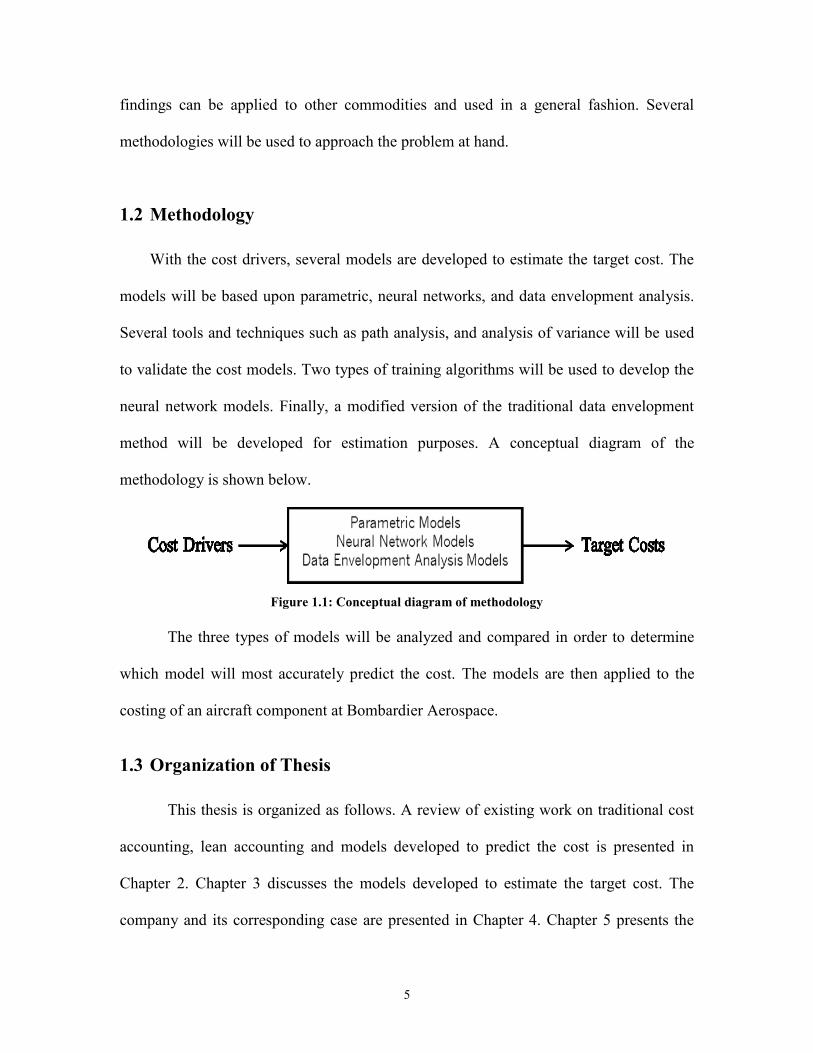
1.2 Methodology
With the cost drivers, several models are developed to estimate the target cost. The
models will be based upon parametric, neural networks, and data envelopment analysis.
Several tools and techniques such as path analysis, and analysis of variance will be used
to validate the cost models. Two types of training algorithms will be used to develop the
neural network models. Finally, a modified version of the traditional data envelopment
method will be developed for estimation purposes. A conceptual diagram of the
methodology is shown below.
Figure 1.1: Conceptual diagram of methodology
The three types of models will be analyzed and compared in order to determine
which model will most accurately predict the cost. The models are then applied to the
costing of an aircraft component at Bombardier Aerospace.
1.3 Organization of Thesis
This thesis is organized as follows. A review of existing work on traditional cost
accounting, lean accounting and models developed to predict the cost is presented in
Chapter 2. Chapter 3 discusses the models developed to estimate the target cost. The
company and its corresponding case are presented in Chapter 4. Chapter 5 presents the

6
results and analysis. The summary of findings, practical application and managerial
implications are presented in Chapter 6. Finally, Chapter 7 presents conclusions and
limitations of the thesis, and discusses potential future research.

7
2. Literature Review
Much research has been conducted on traditional costing methods. According to
Kaplan (1988), a major problem with traditional cost management (accounting) practices
is the incorrect allocation of overhead. Kaplan (1998) states that companies are using
their direct labour to allocate overhead, when in fact the direct labour only represents a
minor portion (about 10%) of the manufacturing costs. The incorrect allocation of costs
can result in losing competitive strategy (Cooper, 1995; Maskell, 1996).
Traditional cost management principles may also misguide many managers due to
the reliance on procedures put in place to reduce the unit cost of a product. As the
overhead will typically be allocated over the total number of units produced, it would
push for the high production of units, with the intent of fully utilizing labour and
machines. Even though, based on cost allocation practices, it would reduce the average
overhead per unit, it would result in over production, hence a great amount of inventory.
Therefore researchers state that traditional methods are appropriate when dealing with
standard mass production industries of the 1960‟s, but not of those today (Johnson and
Kaplan, 1987; Johnson, 1990; Turney, 1991; Johnson, 1992; Maskell and Lilly, 2006;
Stenzel, 2007; Cooper and Maskell, 2008).
Moreover, traditional methods can push management, by not understanding the
cost drivers, to develop products that are over engineered and do not meet the needs of
the customer (Butscher et al., 2000). It can also lead management to develop
performance measures that do not reflect the priority, as they do not focus on the right
things, i.e. the product, its characteristics, and ultimately the customer (Maskell and
Baggaley, 2002).

8
Zbib et al. (2003) summarize the drawbacks of traditional accounting principles
for companies driven by their supply chain. Some of the disadvantages reported are the
following:
1. Do not account for the changes in the cost structure
2. Over emphasize the relevance of direct labour cost
3. Not fully aligned with just in time (JIT) principles
4. Inconsistency in the continuous improvement activities
5. Ignores the needs of the customer
6. Purchasing decision based upon the lowest price
7. Too many suppliers
8. Performance measurements on cost alone, can overlook quality and on time
delivery
Many shortcomings of traditional practices have been highlighted by several
researchers. Fritzch (1998) proposed two methods to establish product cost: activity-
based costing (ABC) and the theory of constraints (TOC). TOC focuses on increasing the
profitability of an organization by adjusting the scheduling to maximize the
manufacturing output (Goldratt and Fox 1992, 1996; Goldratt, 1999). Goldratt and Fox
(1992) argue that focusing on the product cost is a way of the past and the focus should
be on maximizing the throughput (manufacturing production). Their underlying
assumption is that there are negligible (or minimal) variable costs, and the majority of the
costs are fixed.
According to Ifandoudas and Gurd (2010), the premise of the TOC model is to
focus on the global efficiency, rather than any local efficiency. Moreover, they state that

9
the throughput, the inventory, and the operating expense are the measures for activities
for a business using the TOC model. Razaee and Elmore (1997) state that if the TOC
model is properly implemented in an organization, it can result in a reduction in
inventory, lead-time and cycle-time, while increasing the productivity and quality.
However, Kaplan (1998) states that the TOC is flawed due to wrongfully
classifying parameters, such as price and labour rates as fixed costs. Moreover, Kaplan
(1998) challenges the TOC model, due to it conglomerating many of the costs as
operating expenses, which results in a larger portion of unallocated costs then that even
of traditional costing.
According to Fritzch (1998), apart from the TOCs model, the other methodology
of establishing the product cost is activity-based costing (ABC). ABC, also known as
activity-based accounting focuses on the manufacturing processes related to the
development of a product (Johnson and Kaplan, 1997). All the incurred costs from the
direct and indirect processes are allocated to a product to establish its unit cost. Thus,
according to Carmo and Padovani (2012), its objective is to reduce the distortion caused
by arbitrarily allocating the indirect costs. The benefit of ABC is that is provides a
precise view of the consumption of resources by activities, which corresponds to the costs
(Cokin et al., 2012).
Even though the ABC method has overcome some of the obstacles of traditional
accounting, it has its drawbacks. Benjamin et al. (2009) argue that ABC is simply an
extension of traditional accounting, as they state that ABC simply splits (allocates) the
overhead into several bases instead of one, as is the case in traditional accounting. For
this reason, Benjamin et al. (2009) proposed the methodology of efficiency based

10
absorption costing (EBAC). They state EBAC is an improvement to ABC by considering
the element of overhead utilization efficiency when allocating the costs. They define
efficiency as the ratio of input required to produce an output. They further explain the
efficiency rate as a division of the number of cost drivers of a particular product, by the
number of units produced thereof.
Other researchers such as Womack and Jones (1996), who are strong promoters of
lean manufacturing, have also questioned the principles of ABC. They argue that it
requires many resources to implement, and is costly to maintain. Furthermore, they state
as ABC will solely focus on cost minimization, it will not focus on continuous
improvement, waste reduction, and most importantly, the customer and the value created
for them. Finally, they state that ABC is simply another method of allocating costs, which
is a pivotal flaw in the principles of traditional accounting.
Some of the shortcomings of traditional accounting have been overcome through
the use of lean manufacturing principles. Lean manufacturing has had great success in
production environments (Lander and Liker, 2007) through a focus on the creation of
value through the elimination of waste. Taichi Ohno (1912 - 1990) was a Toyota
executive who had identified seven types of deadly wastes, which are referred to as muda
in Japanese. The seven wastes are: Excessive Motion, Waiting Time, Over Engineering,
Unnecessary Processing Time, Defects, Excessive Resources and Unnecessary Handoffs
(Womack and Jones, 1996). The objective of lean is to act as an antidote to eliminating
these wastes. Oakland and Marosszeky (2007) quote James Womack, president and
founder of Lean Enterprise Institute, who said, “None of us have seen a perfect process,
nor will most of us ever see one. Lean thinkers still believe in perfection, the never
11
ending journey towards the truly lean process.” Womack and Jones (1996) defined the
five basic principles of lean; Value, Value Stream, Flow, Pull, and Perfection. Since the
focus of lean thinking is on the customer, it is important to understand what the customer
perceives as value. After the value to the customer is identified, the value stream of the
product should be identified. The value stream includes taking a product through the
design, make and order phase. All the processes in the value stream should flow to avoid
interruptions. Wherever continuous flow is not possible, a pull system should be
introduced. The pull system is created so that a product is produced just in time, when it
is required from the customer. Lean principles are a continuous process of improvement
which always seeks the fifth principle, perfection. In short, lean thinking is employed
because it provides a method to do more with less (Womack and Jones, 1996).
More recently, the success of lean manufacturing principles has led to their
application in other areas of the enterprise, such as to the supply chain (Miao and Xu,
2011), engineering (Black and Philips, 2012; Beauregard, 2010; Schulze and Störmer,
2012) and even accounting (DeBusk, 2012).
DeFilippo (1996), Womack and Jones (1996), Maskell and Baggaley (2002),
Cooper and Maskell (2008), and Bahadir (2011) indicated the urgency of aligning
accounting principles with a lean philosophy. Lean accounting focuses on eliminating
waste in the accounting process. There are many sources of such waste such as
unnecessary transactions, meetings, and approval processes that are time consuming,
costly and serve no value (Maskell and Lilly, 2006). Some of the many benefits of lean
accounting that Maskell and Baggaley (2004) stated are the following:
1. Provides information in order to make better (lean) decisions
12
2. Eliminate redundant systems and unnecessary transactions which will reduce
time and cost
3. Provides information and statistics focused on lean
4. Directly addresses customer value
Ward and Graves (2004) in conjunction with the UK Lean Aerospace Initiative
(UK LAI) developed a theoretical framework for supporting lean thinking with respect to
cost management in the following three dimensions:
1. Manufacturing
2. Extended Value Stream
3. New product introduction
In the dimension of manufacturing, they identified the following three parameters
for consideration.
1. Product costing and overhead allocation
2. Operational control
3. Costing for continuous improvement
They proposed using the notion of value stream costing, the process of allocating all the
costs to the product or value stream, rather than a department (Stenzel, 2007).
Furthermore, for operational control, they proposed using lean performance measures,
such as the takt time, which, also referred to as the output rate, is the synchronization of
the paces of different processes (Seth and Gupta, 2005). Ward and Graves (2004)
discussed several techniques such as kaizen costing, cost of quality, cost of waste, and

13
activity based costing for continuous improvement, where kaizen costing refers to finding
opportunities and proposing alternative techniques for the manufacturing of the part to
reduce the cost (Mondem and Hamada, 1991). Wang (2011) describe the two elements of
kaizen costing being the accounting and physical control system. The accounting control
systems are those of continuously setting and deducing cost reduction targets, whereas
the responsibility of achieving the targets and placed upon the shop floor, is known as the
physical control system. As kaizen costing focuses on the continuous reduction in cost, it
is aligned with the principles of lean accounting (Modarress et al., 2005).
In terms of the extended value stream, which is the entire supply chain from raw
material provider to the end customer (Womack and Jones, 2003), they (Ward and
Graves, 2004) proposed kaizen costing and target costing (TC) with the intent of reducing
the costs. Similarly target costing along with life cycle costing, was proposed for cost
management techniques for the introduction of new products.
Target costing originated in Japan in the 1960‟s (Ellram, 1999; 2000; 2006) and
was originally known as Genka Kikaku (Nicolini et al, 2000). Target costing is defined as
a methodology of using a systematic process of managing the cost of a product during its
design phase (Ibusuki and Kaminski (2007); Iranmanesh and Thomson (2008); Ax et al.,
(2008); Filomena et al. (2009); and Kee (2010). Target costing is more simply defined as
the process of deducing the target cost (TC) from the difference of desired target profit
(TP) and the target price (T-Price) of the market (ie. TC = TP – T-price). The TC is
defined as the financial goal of the full cost of a given product, from derived from the
estimate of its selling and the desired profit (Rhodes et al., 2006). Ulrich and Eppinger
(2012) define TC as the manufacturing cost at which a company and all of its associated

14
stakeholders for the given distribution channel, while make sufficient profit at a
competitive price. Yazdifar and Askarany (2012) summarize the two objectives of target
costing as:
1. Reducing the cost of the new product so the required amount of profit can be
achieved (Target Profit = Target Price – Target Cost). Furthermore, this is to
be coupled with satisfying the following three conditions
i. Quality
ii. Development time
iii. Price demanded from the global market
2. Motivating employees up front, during the development phase, to achieve the
target profit.
As the intent of TC is to reduce the cost to obtain the target profit, it has been
applied in many domains. Some of the recent research in TC has been in the domains of
IT (Choe, 2011), construction (Pennanen et al., 2011; Chan et al. 2010; 2011), rail
transportation (Mathaisel et al., 2011), food (Bertolini and Romagnoli, 2012), automotive
(Slater, 2010), and aerospace (Bi and Wei, 2011).
According to Lorino (1995), over 80% of the large Japanese assembly companies
had adopted TC. This is not the case in the rest of the world. According to a recent study,
Yazdiffar and Ashkarany (2012) conducted a study on manufacturing firms in Australia,
New Zealand, and the United Kingdom, and found that less than 20% of the firms
adopted the practice of TC.

15
Jenson et al. (1996) studied several case studies and found that those that
incorporated lean accounting principles to pursue excellence all possessed the following
characteristics:
1. Integration of business and manufacturing cultures
2. Recognized lean manufacturing and its effect of management accounting
3. Emphasize on continuously improving their accounting methods
4. Strive to eliminate waste in accounting
5. Encourage a pro-active management culture
Maskell (1996, 2000) developed a theoretical framework to show how companies
adopting the principles of lean can move away from the traditional cost management
techniques. Maskell‟s 4-Step lean accounting maturity model provides a framework that
shows the various levels of maturity of organizations incorporating lean costing
principles.
The first level of maturity is to address the low-hanging fruit in which current
accounting and control system is maintained by minimizing waste from the system.
Secondly, by removing unnecessary transactions, the redundant cost of excessive
financial reporting will be eliminated. Thereafter the 3rd
level of maturity will eliminate
waste. The operations are independent from the accounting reporting periods. Finally, the
fourth level of maturity is lean accounting. It focuses on minimizing transactions such as
in product completion and product shipment.
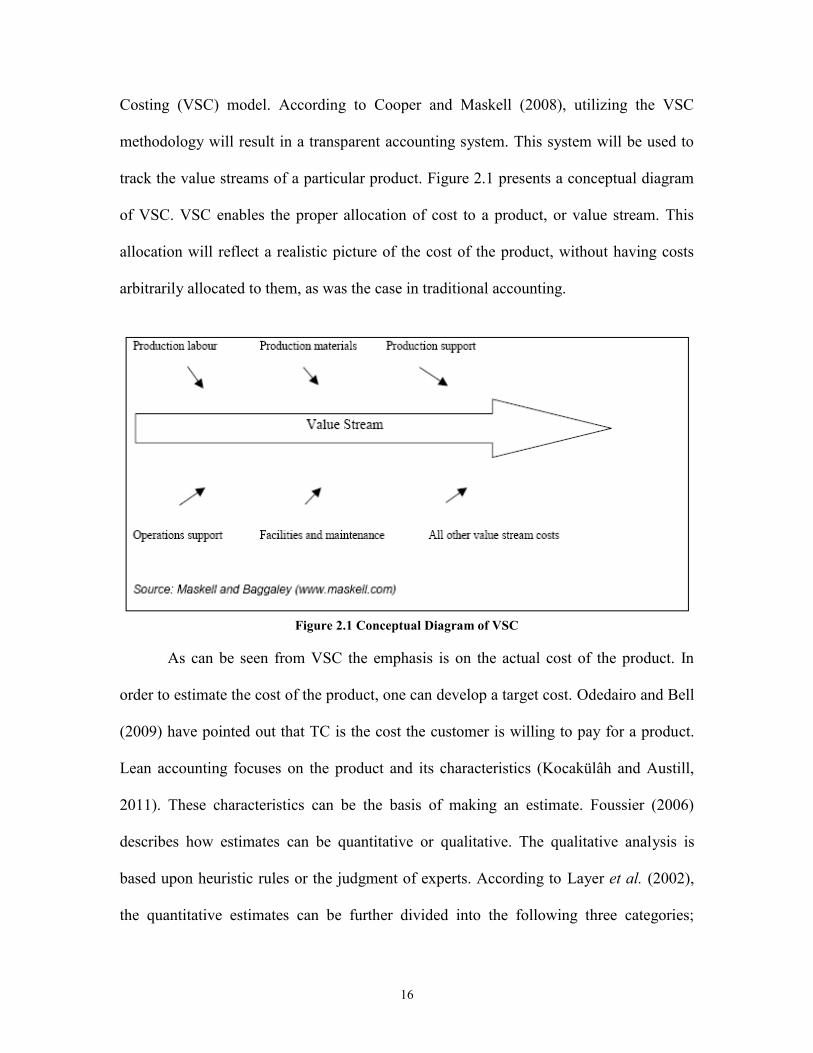
Other more recent models have been developed based on the principles of lean.
Gamal (2011) applied the principles of lean accounting to develop a Value Stream
16
Costing (VSC) model. According to Cooper and Maskell (2008), utilizing the VSC
methodology will result in a transparent accounting system. This system will be used to
track the value streams of a particular product. Figure 2.1 presents a conceptual diagram
of VSC. VSC enables the proper allocation of cost to a product, or value stream. This
allocation will reflect a realistic picture of the cost of the product, without having costs
arbitrarily allocated to them, as was the case in traditional accounting.
Figure 2.1 Conceptual Diagram of VSC
As can be seen from VSC the emphasis is on the actual cost of the product. In
order to estimate the cost of the product, one can develop a target cost. Odedairo and Bell
(2009) have pointed out that TC is the cost the customer is willing to pay for a product.
Lean accounting focuses on the product and its characteristics (Kocakülâh and Austill,
2011). These characteristics can be the basis of making an estimate. Foussier (2006)
describes how estimates can be quantitative or qualitative. The qualitative analysis is
based upon heuristic rules or the judgment of experts. According to Layer et al. (2002),
the quantitative estimates can be further divided into the following three categories;

17
analytical, analogous, and statistical models. The statistical models contain both
regression models (RM) and models using neural networks (NN).
In recent years, research has been conducted on cost estimation using both RM
and NN. Salam et al. (2008, 2009) developed RM using both linear and non-linear
models to estimate the design effort for an aircraft component. The estimated cost can
easily be derived by multiply the effort by the labour rate. Furthermore they utilized the
jackknife technique, which is a sub-sampling technique to reduce the bias. Moreover, an
analysis of variance (ANOVA) was conducted to determine the significant cost drivers. It
was found the estimate based upon a non-linear model yielded better results.
Sayadi et al. (2012) conducted a comparative study between single point and
multiple non-linear (NL) RM. Their findings were that the NL RM has a better outcome
to predict the costs.
Caputo et al. (2008) compared the use of NN models trained using back
propagation, to that of a non-linear regression model to estimate the cost of a pressure
vessel. The term training using back-propagation (BP) refers to a systemic process of
adjusting the weights of the NN in order to reduce the square error (Pandya and Macy,
1996). They found the estimation based upon NN to outperform those using the non-
linear regression model. They as well as Chou et al. (2010) pointed out the requirement
of a large sample size in order to have meaningful results using NN.
Chou et al. (2010) conducted a comparative analysis of RM to NN trained using
BP to NLM, In order to estimate the development cost of manufacturing equipment.
Their findings, similar to Caputo et al. (2008), was that the NN models using BP

18
outperforms the NLM. In recent years, other researchers, such as Ju and Xi (2008) and
Zangeneh et al. (2011) have used the NN trained using BP to estimate the cost.
NN can also be trained using the genetic algorithm (GA). Even though the NN
based upon GA have been used in many domains, there is little literature found on
comparing the use of the GA versus BP for the training algorithm on cost estimation.
Table 2.1, summarizes the research found on comparing the methodologies of
cost estimation, as well as the tools and techniques they used for estimation thereof, and
shows the analysis to be conducted in this thesis.
Table 2.1: Comparison of developed models
As there has not been research conducted using an exhaustive approach to
compare all estimation techniques, this thesis takes a holistic approach by using the
above-mentioned methods to estimate target costs. It will also present a complex non-
linear model (CNLM) used to estimate the cost. Furthermore, it will discuss the
development of an adapted mathematical model, namely data envelopment analysis,
which is typically used to calculate efficiency; however it is modified to serve as a target
costing model. All models will be applied in a case study on a commodity in the
aerospace sector.
Linear
Model
Non-Linear
Model
NN trained
using BP
NN trained
using GA
Thesis‟ models and techniques
Salam et al. (2008; 2009)
Sayadi et al . (2012)
Caputo et al. (2010); Chou et al . (2010)
Ju and Xi (2008), Zangeneh et al. (2011)

19
3. Target Costing Models
In this chapter, the models developed to estimate the targets costs are described in
detail. There are three types of models that are developed. This first type is a parametric
cost estimation model. Two types of regression models and a complex non-linear model
are developed. The second model is based on neural networks. Two types of neural
network models relying on different training algorithms are presented. Finally, the third
model presented is a data envelopment analysis model.
3.1 Parametric Cost Estimation
Parametric cost estimation is a technique that can be used to develop a cost
estimate based on the statistical relationship of the input variables, (PMI, 2000; ISPA,
2009). Parametric cost estimation has many applications. It is a tool that is deemed
essential for project management (PMI, 2000). In the context of projects, parametric
estimation determines estimates for parameters (e.g. cost or duration) using historical
data and/or other variables. It can be used to determine the feasibility of a project, to
determine a budget, and to compare projects (products), amongst others (Fragkakis et al.,
2011). The input variables, which are the cost drivers, will be used to formulate the cost
model or the cost estimating relation (CER). The parametric CERs are commonly utilized
to estimate the cost during the design phase of a product, when only the few, yet key
design parameters or input variables (in this case, cost drivers) are known. CERs can be
parametric or non-parametric. The generic formula is as follows:
CER (y) = f(xi) (3)

20
The CER, or the target cost is a function of its input variable(s). CERs can be
simple or complex. The simple CERs depend on a single cost driver, whereas the
complex CERs depend on multiple cost drivers (ISPA, 2009). By identifying the cost
drivers, parametric models can be developed. Parametric models can be linear, non-
linear, log-normal, and exponential, amongst others.
In this thesis, two models based on linear regression are selected to formulate the
CER. The reason for selecting the regression models are because they are commonly used
in practice today, and they will formulate the basis of comparison to the other more
complex models developed and discussed in the sections to come.
The simple CER based on a linear regression (LR) model can be denoted as
following.
(4)
where,
y, Target cost
β0, Intercept
β1, Slope
X1, cost drivers
ε, Error
As can be seen, the element of error is introduced. The error, or noise, represents
the element of the cost not described by its cost driver. As can be seen from the standard
form there is only one independent variable, hence only one cost driver. However in
many cases, such as that of this case study, several cost drivers are selected, thus the CER
110 Xy
21
will be complex. The complex form of the CER using regression can be denoted by the
multiple linear regression model (MLRM). The MLRM function is as follows:
(5)
where,
y, Target cost dependent on k predictor values
βj , Regression coefficients
Xk, kth
independent variable
ε, Error
The regression coefficients are deduced by the method of least squares. The least
squares estimation generates an equation that will minimize the sum of the square errors
(Kutner et al., 2004). As the method of least squares has been commonly used for several
years, it will not be further described.
Another complex CER will be developed based upon a standard non-linear model
(NLM). The purpose of developing another parametric CER will be used as a comparison
mechanism to that based upon the MLRM, in terms of accuracy of prediction. In
statistics, the NLM is a type of regression that utilizes data modeled in the form of non-
linear combinations (Montgomery, 2005). Below is the formula for the NLM used in this
study.
(6)
where,
, Target cost
Xm, Specified cost driver
βm, Regression coefficient
kk XXXy ...22110
321
3210ˆ
XXXy

22
Since Equation (6) is represented in a non-linear form, it must be transformed into
a linear model to conduct the regression analysis. The manner to transform the model in a
linear form is simple, the natural log (ln) on both sides of the equation are taken. The
resulting equation will thus be suitable for linear regression. The linear equation
generated is shown below.
ln = ln (βo) + β1 ln (X1) + β2 ln (X2) + β3 ln (X3) (7)
Thereafter, as the equation is in the standard linear regression form, the least
squares method will be utilized to calculate the regression coefficients. As the units for
the input and output variables are not identical, the units will have be addressed, and this
will be done through dimensional analysis. Dimensional analysis is a tool used to verify
relations between physical quantities by checking their dimensions (Palmer, 2008). In the
case where all the input variables do not have the same units, the simplest way to remove
them would be to divide each input value by a reference value of unity having the same
units. The procedure would be the following.
Step 1
Categorize all the input data, by their given dimensions.
Step 2
Divide all the reference data of the ith
variable for sample n, with dimension di by the
reference value of 1 having the same di.
(8)
If this procedure is repeated for all the variables, none of the values will have any
dimensions, hence be dimensionless. The analysis can be carried out without the
constraint of different dimensions of variables.
23
Even though the units have been removed using the dimensional analysis technique, the
models are linear. As the models described in Section 3.1 are based upon linear
regression, it is important that the linearity and normal assumptions are met.
3.1.1 MLRM Assumptions
In order to use the MLRM the following two assumptions need to be satisfied.
1. Linearity assumption
2. Normality assumption
3.1.1.1 Linearity assumption
In order to determine if the function is linear for a given case of the MLRM,
scatter plots or residual plots can be made. In the case of the scatter plot, the standardized
residuals could be plotted against the non-standardized predicted value. For a linear
function, the scatter plot should not have any curvilinear patterns.
Another graphical manner to statistically prove the validity of the MLRM is to
create statistical process control (SPC) charts. In the context of this research, the
predicted values against the actual values of target cost will are plotted. The errors or
residuals will be the deviation from the line ln (Predicted) = ln (Actual) + ε. The expected
error, assuming a normal distribution, is zero, i.e. E (ε) =0. Thus, the mean of the
function f(x), will simply be f(x). The equations for the upper control limits (UCL) and
lower control limits (LCL) are shown below.
UCL = f(x) + 3ζ (9)
LCL = f(x) -3ζ (10)

24
where,
f(x), Masked Cost = Target Cost + ε
ζ, Standard deviation of the residuals
As can be seen from equations (9) and (10), the notion of masked cost is
introduced. As can be understood, Bombardier, similar to any other company, is sensitive
to proprietary information. The company will not divulge the commercial terms they
have with their suppliers. On the other hand, it is important for the regression to have
meaningful results. Thus, the use of a proper data masking technique is important. A
masking technique described by Muralidhar et al. (1999) was applied to the company raw
data and will be described in a later section.
According to Montgomery (1985), if the residuals are within 3ζ of the expected
value of the function, then the function is considered to be statistically in control. In other
words, the assumption of linearity holds.
3.1.1.2 Normality assumption
The second assumption that must be validated is that the error values follow a
normal distribution. The test to determine error normality requires the coefficient of
correlation, r. The value of r is calculated from the following equation.
(11)
where,
R2, Coefficient of determination
The value of R2 is calculated from the following equation.
(12)
2R r
SSTO
SSR 2 R
25
where,
SSR, Regression sum of squares
SSTO, Total sum of squares
This will also involve a hypothesis test in which the critical values for the
correlation coefficient, prepared by Looney and Gulledge (1985) are to be compared
against the resulting correlation coefficient, r, from the generated regression model. The
Ho assumes the error has a normal behaviour. The H1 assumes the error not to have a
normal behaviour. The outcome of the test is as follows:
(13)
In contrast to Looney and Gulledge (1985), derived from ISPA (2009), if the
value of r is greater or equal to ~0.837 (R2 ≥ 0.70) the model is good, whereas if the value
of r is between ~0.592 and ~0.837 (0.35 ≥ R2 0.70) the model has marginal results.
Anything below the previous mentioned values for r would not be considered as an
acceptable value, highlighting little worth of the generated model. These values will be
used to fulfill the normality assumption.
As previously mentioned, the regression model uses the method of squares for
error to calculate the regression coefficients. It is therefore understood that the more data
points available for the model, the more robust the generated model will be. However, as
this methodology is being applied in a case study at BA, there are limited data points, 13
to be precise. The manner of overcoming this constraint is by creating more data points.
In order to do this, a sub-sampling technique, namely the jack knife technique, is utilized.
Lr
1
0
H conclude ),-(1 If
H conclude ),-(1r If
L
L
rr
r
26
3.1.2 Jackknife Technique
The jackknife technique is used to determine the regression coefficients of each of
the model parameters. This technique was originally a computer-based method for
estimating biases and the standard errors. According to Efron and Tibshirani (1993), this
technique is commonly used not only to improve the problem of biased estimation due to
small sample size, but also in situations where the distribution of the data is hard to
analyze. In this technique, the data are divided into sub-samples, and the sub-samples are
obtained by deleting one observation at a time. The calculations are carried out for each
sub sample. Given a data set x = (x1, x2, x3,…,xn), the ith
jackknife sample xi is defined to
be x with the ith
data point removed. The pseudo-values, Psi, are determined using the
following equation:
(14)
where,
Psi, Pseudo-value for the entire sample, omitting sub-sample i.
ns, Number of sub-samples
, Least-squares estimator of the whole sample
Least-squares estimator for the entire sample, omitting sub sample i
The jackknife estimator is determined as follows:
(15)
i-β)1(β nsnsPsi
β
,β i-
β~
ns
Psns
i
i 1~

27
3.1.3 Selection of Cost Drivers for the Final Regression Model
This section discusses two techniques that determines which selected cost drivers
will be kept in the final CERs, one for the MLRM, and the other for the adapted version
of the NLM. The techniques are path analysis (PA) and analysis of variance (ANOVA).
The first technique, PA, is very visual. It is usually used to reduce the number of
selected cost drivers to keep in the final CER, with the intent of ensuring that the model
has meaningful results. It will result in showing the individual effects of each of the cost
drivers, and how they interact with one another, and with the cost. Contrary to PA,
ANOVA will not try to minimize the number of cost drivers. Rather, it will only retain
the selected cost drivers that are statistically significant in the final regression model.
3.1.3.1 Path Analysis
Path analysis, developed by Wright (1934), was an approach used to study the
direct and indirect effects of variables. This approach takes a confirmatory, rather than
exploratory, approach to data analysis and requires that the inter-variable relations be
specified beforehand. This type of model will enable one to understand the effects that
each of the cost drivers will have on the output of the equation. Therefore, in this applied
research, the PA model will determine the direct impact and indirect impact that the cost
drivers have on the target cost. The reference to the impacts will be denoted as path
coefficients from this point onwards. A conceptual diagram of the PA model can be seen
in Figure 3.1 below.

28
Figure 3.1: Conceptual PA diagram
As can be seen in Figure 3.1, xi represents the cost drivers. The circle containing
the letter “y” represents the dependent variable, the cost. The circles containing the letter
“U” represents the un-correlated value of the function. The term correlation refers to
dependency of a variable on another one. As previously mentioned, the path coefficients,
p0i are the direct and indirect effects that the independent variables have on the output of
the equation. The inter-relationships (rij) that can be seen in Figure 3.1 are simply the
correlations of the factors (cost drivers and cost), which can be derived from the
correlation matrix. The correlation matrix for the conceptual PA presented in Figure 3.1
is depicted in Table 3.1 below.
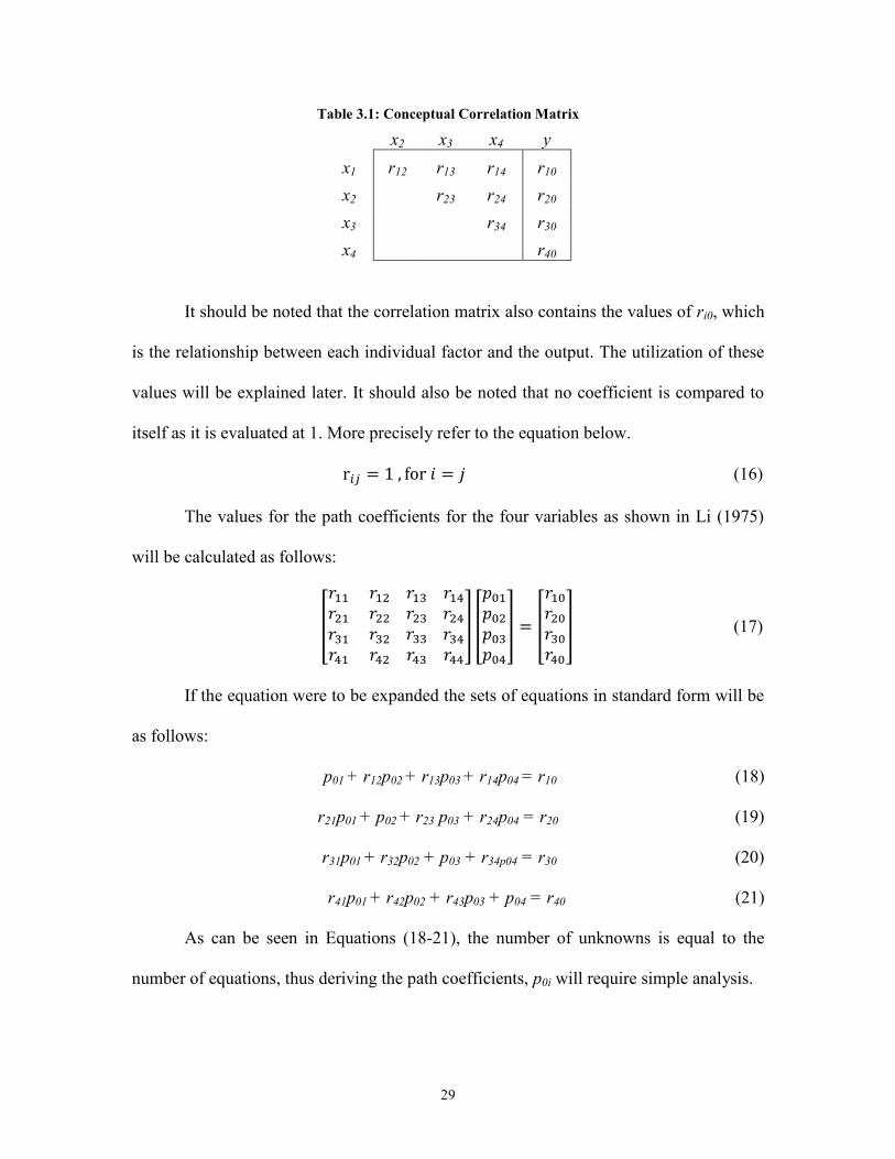
29
Table 3.1: Conceptual Correlation Matrix
x2 x3 x4 y
x1 r12 r13 r14 r10
x2 r23 r24 r20
x3 r34 r30
x4 r40
It should be noted that the correlation matrix also contains the values of ri0, which
is the relationship between each individual factor and the output. The utilization of these
values will be explained later. It should also be noted that no coefficient is compared to
itself as it is evaluated at 1. More precisely refer to the equation below.
(16)
The values for the path coefficients for the four variables as shown in Li (1975)
will be calculated as follows:
[
] [
] [
] (17)
If the equation were to be expanded the sets of equations in standard form will be
as follows:
p01 + r12p02 + r13p03 + r14p04 = r10 (18)
r21p01 + p02 + r23 p03 + r24p04 = r20 (19)
r31p01 + r32p02 + p03 + r34p04 = r30 (20)
r41p01 + r42p02 + r43p03 + p04 = r40 (21)
As can be seen in Equations (18-21), the number of unknowns is equal to the
number of equations, thus deriving the path coefficients, p0i will require simple analysis.
30
Building on the work of Wright (1934), Li (1975) derived another manner to
calculate the path coefficients. The derived equation is as follows:
(22)
where,
ai, Regression coefficient of the independent variable i
ζi, Standard deviation of the sample data of the independent variable i
ζy, Standard deviation of the sample data of the dependent variable
If Figure 3.1 representing the conceptual PA diagram is recalled, the variable U
represents the un-correlated value of the function. The value of path coefficient, p0U is
calculated from the following equation:
(23)
where,
ζy, Standard deviation of the ith
cost driver
ζe, Standard deviation of the residuals
The residuals, ei are calculated from the following equation.
(24)
where,
yn, Actual cost for sample number n
, Output (predicted cost) value for sample number n
It should be recalled that the predicted value of the output will be obtained from
the resulting CER derived from Equation (5) for the standard MLRM and from Equation
(7) for the MLRM that was transformed from a non–linear state.

31
The variance, ζ2 refers to the measuring the spread out the data. The total variance
of the actual cost is a combination of the variance of the predicted cost and the variance
of the residuals. This is mathematically represented in Equation (25).
(25)
where,
, Variance of the sample data of the dependent variable
, Variance of the predicted output value
, Variance of the residuals
Once the variance and the path coefficients are obtained, the total effect that the
cost drivers have on the predicted cost can be calculated from either one of the following
equations.
(26)
(27)
As can be seen from the notation, the total effect the cost drivers have on the
predicted cost is simply the coefficient of determination derived from the linear
regression model.
The PA model can serve as a tool to try to reduce the number of cost drivers,
while still having meaningful results. Keeping this objective in mind, the first step would
be to see if the model can be based solely upon a single cost driver. The procedure is as
follows:

32
Step 1
Having the data readily available is important. One would refer to the correlation matrix.
In this case, for the conceptual model, this could be found in Table 3.1
Step 2
In order to pick the best cost driver, the single cost driver that has the greatest effect on
the predicted cost, in other words, the variable with the greatest value of riy, is selected.
Step 3
As only 1 cost driver is considered at this point, the new value of R2 is calculated from
the following equation.
( )
(28)
Step 4
The next step requires intuition to determine if the revised R2 is still acceptable. This
could be calculated as a percent change of the previous value, or it also could be based
upon a certain threshold value for R2 as shown in ISPA (2009) or derived from Looney
and Gulledge (1985). There could also be other methods adopted in industry to be
utilized depending on the context and application of the model.
Step 5
If the resulting R2 value is acceptable based upon an established acceptance criteria, the
resulting model will be solely be based upon a cost driver. However, if the resulting
model is not acceptable the PA has to be recomputed by adding another factor. The next
best cost driver identified in Step 2 should be selected.

33
Step 6
Repeat Step 1 to Step 5 until an acceptable value of R2, as described in Step 4, is
obtained. It should be noted that this procedure may repeat several times. Even though
PA may keep or eliminate cost drivers, it does not indicate whether the cost drivers are
significant. In order to determine the significant cost drivers, further analysis must be
conducted, and this is done in this research using ANOVA.
3.1.3.2 Analysis of Variance
ANOVA for an MLRM will help to determine which cost drivers have a
statistical significance (Kutner et al., 2004). The ANOVA will indicate, with the use of
the F-test for linear regression, if the CER only contains statistical significant cost drivers
(Weisberg, 2005). When conducting a regression analysis on computer software as
Microsoft Excel, the ANOVA table can be automatically generated by utilizing the
statistical application. The ANOVA table would include the p-value for any given
regression coefficient (cost driver). According to Kutner et al. (2004), the p-value will
indicate the statistical significance of a given parameter, which in this case, the cost
drivers. The following set of equations will be utilized to determine if the selected input
variables are statistically significant.
(29)
(30)
For the purpose of this thesis, the selected confidence level, which would relate to
the reliability of the estimate, is set at 90%. It should be noted that the subscript, i for the
term, pi represents the ith
cost drivers, as several cost are considered in the complex CER.

34
After creating the regression model and computing the ANOVA, if there is a
single value of pi > 0.1, the regression will have to be repeated by eliminating the
selected cost driver with the greatest value of pi. This procedure will repeat itself until the
all the values of pi ≥ 0.1. The resultant equation will be utilized to predict the target cost
solely upon statistically significant cost drivers at a specified confidence level, 90% in
this case.
All the tools and techniques discussed in the previous sections will be used to
support the methodology of linear regression. However, it only compares the standard
MLRM and a simple non-linear model for the development of a cost model. A more
complex parametric CER to be used for estimating the target cost is referred to from this
point forward the complex non-linear model.
3.1.4 Complex Non-Linear Model
The CNLM used in this thesis has the following notation.
(31)
As was the case in the regression models, the terms xi represent the cost drivers,
and remaining terms are the constants. As this equation is not in the form of a regression
model, the constants will have to be determined analytically. The manner is determining
the constants will be using the gradient descent algorithm (GDA). The GDA is an
optimization tool to find the local minima of a function (Snyman, 2005). In order to
determine the constants, the function to be minimized is the square error of the predicted
versus the actual costs (ie. ∑ ). The gradient, for each of the constants will
calculate the amount the constant has to be changed (ie. delta) in order to minimize the
function, the square error. Furthermore, the value of the constant will be adjusted by

35
multiplying it by a step rate, η. Each of the constants will be adjusted each iteration until
the specified stopping criterion (ie. acceptable change in error) is fulfilled.
Parametric CERs depend on a pre-determined cost function to establish the target
cost. However, using non-parametric models such as the models based upon artificial
intelligence, such as neural networks (NN) does not require pre-determined relationships.
NN models have the ability of self-determining relationships of the variables to predict
the cost. Therefore, the next model developed is based upon NN, and is discussed in the
following section.
3.2 Neural Networks
Neural networks (NN) traditionally refer to a network of biological neurons that
are functionally related in the central nervous system. Neural networks may be used for
solving artificial intelligence problems without necessarily creating a model of a real
biological system (Pandya and Macy, 1996). Since biological neural networks are quite
complex, the term artificial neural networks (ANN, or simply NN) is used when a
somewhat simplified version is studied. They are nevertheless used to model complex
relationships between inputs and outputs in an effort to find data patterns. A NN is
essentially a number of interconnected elements that work together to solve a problem.
Through a learning process, whereby it learns by example, it can be configured for a
specific application. They can be utilized in many applications, such as data processing,
classification, and function approximation to name a few (Pandya and Macy, 1996,
Bishop, 1996).
Several researchers such as Tu (1996), Cavalieri et al. (2004), and Caputo (2008)
have commended neural networks (NN) models for their ability to characterize complex
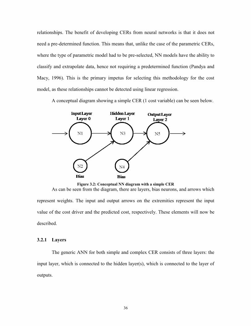
36
relationships. The benefit of developing CERs from neural networks is that it does not
need a pre-determined function. This means that, unlike the case of the parametric CERs,
where the type of parametric model had to be pre-selected, NN models have the ability to
classify and extrapolate data, hence not requiring a predetermined function (Pandya and
Macy, 1996). This is the primary impetus for selecting this methodology for the cost
model, as these relationships cannot be detected using linear regression.
A conceptual diagram showing a simple CER (1 cost variable) can be seen below.
Figure 3.2: Conceptual NN diagram with a simple CER
As can be seen from the diagram, there are layers, bias neurons, and arrows which
represent weights. The input and output arrows on the extremities represent the input
value of the cost driver and the predicted cost, respectively. These elements will now be
described.
3.2.1 Layers
The generic ANN for both simple and complex CER consists of three layers: the
input layer, which is connected to the hidden layer(s), which is connected to the layer of
outputs.

37
Input layer: For this problem, an input vector representing the cost driver is
incident to the input layer. This represents the raw information that is fed into the
network.
Hidden layer: The input layer is distributed (or sends data) to the hidden layer.
What goes on in this layer depends on the input and the weights on the connection
between the input and hidden units.
Output layer: The hidden layer is distributed to the output layer via weighted
connections, and what goes on in this layer depends on the hidden units and the weights
between the hidden and output units.
3.2.2 Weights
The weights are the links between the layers. All the neurons have input vectors
containing the weight the exception of the bias neuron. The bias neuron tries to influence
the desired output by shifting the value of the activation function, which will be discussed
shortly, to output values close to those provided in the training data. According to
Kecman (2001), without the element of the bias, the training mechanism may be
impeded, or even stopped (Kecman, 2001).
Figure 3.2 presented a conceptual model of a simple NN CER. A complex CER is
shown in the following diagram.

38
Figure 3.3: Conceptual NN diagram with a complex CER
As can be seen from the diagram, there are 3 input vectors, representing 3 cost
drivers, as in this case. Moreover, the number of neurons in the hidden layer has
increased to 5 excluding the bias neuron. The number of neurons in the hidden layer has
to be determined by trial and error. Thus, a sensitivity analysis is conducted to determine
the number of neurons to use. The output of every vector is calculated using an activation
function.
3.2.3 Activation function
All the neurons in the network, with the exception of the bias, operate by taking
the sum of its weighted inputs and passing the result through a nonlinear activation
function. The non-linear activation function is mathematically computed as follows.
(32)
In this equation, outi,l is the output of ith
neuron in layer l, wj,i,l is the weight for the
connection between jth
neuron of layer l-1 and ith
neuron of layer l, and f is a nonlinear
activation function. There are several conventionally used choices for this activation
Input Layer Layer 0
Hidden LayerLayer 1
Output LayerLayer 2
wj ,i,1 j,i, 2w
Bias
Bias
j
ljlijili outwfnetfout 1,,,, )(
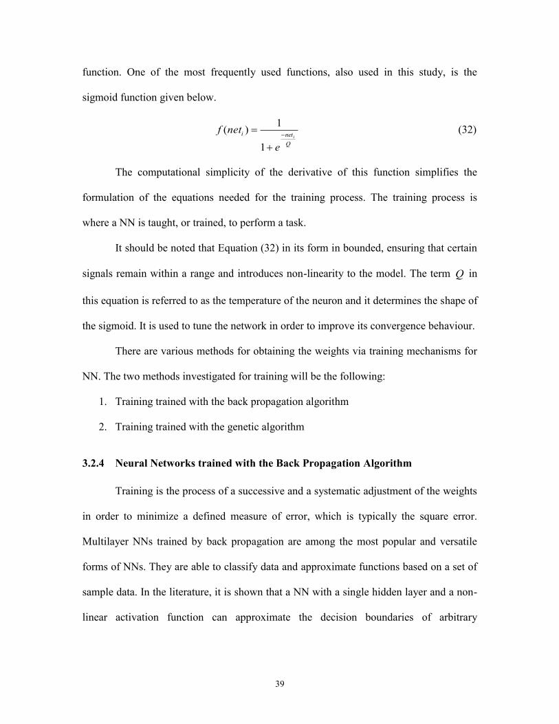
39
function. One of the most frequently used functions, also used in this study, is the
sigmoid function given below.
(32)
The computational simplicity of the derivative of this function simplifies the
formulation of the equations needed for the training process. The training process is
where a NN is taught, or trained, to perform a task.
It should be noted that Equation (32) in its form in bounded, ensuring that certain
signals remain within a range and introduces non-linearity to the model. The term in
this equation is referred to as the temperature of the neuron and it determines the shape of
the sigmoid. It is used to tune the network in order to improve its convergence behaviour.
There are various methods for obtaining the weights via training mechanisms for
NN. The two methods investigated for training will be the following:
1. Training trained with the back propagation algorithm
2. Training trained with the genetic algorithm
3.2.4 Neural Networks trained with the Back Propagation Algorithm
Training is the process of a successive and a systematic adjustment of the weights
in order to minimize a defined measure of error, which is typically the square error.
Multilayer NNs trained by back propagation are among the most popular and versatile
forms of NNs. They are able to classify data and approximate functions based on a set of
sample data. In the literature, it is shown that a NN with a single hidden layer and a non-
linear activation function can approximate the decision boundaries of arbitrary
Q
netii
e
netf
1
1)(
Q

40
complexity (Kecman, 2001). In this thesis, this property is used to investigate the
applicability of neural networks for cost estimation of a major aircraft component.
For the NN to be able to predict the cost given the selected cost drivers as inputs,
it must first be trained using a training set. In the training process, each time an input
vector p (the three cost drivers) from the training set is presented to the network, the
difference between the desired and the actual output is computed and the each weight is
adjusted by an amount ∆wj,i,l, given in Equation (33).
(33)
In this equation, η refers to the learning rate; op,j,l refers to the output of the jth
neuron of layer, l; and δp,j,l refers to the error signal at the jth
neuron of layer l. The error
signal is computed using Equation (34) for the neuron in the output layer and using
Equation (35) for the neurons in the hidden layer. The term tp,1,2 in Equation (34) is the
desired value at the neuron in the output layer (layer 2), corresponding to the pth
presentation of the vector from the training set.
(34)
(35)
This training algorithm is called “training by back-propagation,” and the complete
derivation of the algorithm can be found in Pandya and Macy (1996).
3.2.5 Neural Networks trained with the Genetic Algorithm
Genetic algorithm (GA) was introduced in the 1970s by Holland (1975) has
gained increasing popularity in solving many optimization problems. It is an iterative
procedure maintaining a population of structures (chromosomes) that encode candidate
lipliplij Ow ,,,,,,
)1()( 2,1,2,1,2,1,2,1,2,1, ppppp OOOt
)1( 2,1,2,1,1,,1,,1,, jpjpjpjp wOO
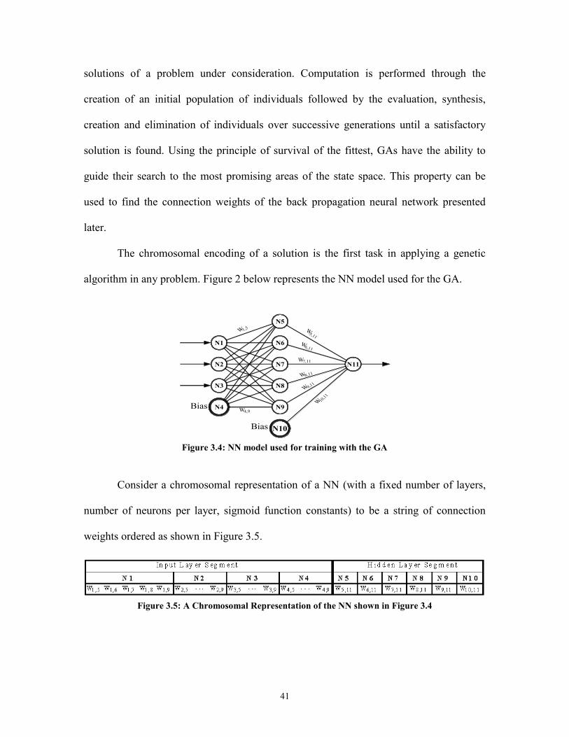
41
solutions of a problem under consideration. Computation is performed through the
creation of an initial population of individuals followed by the evaluation, synthesis,
creation and elimination of individuals over successive generations until a satisfactory
solution is found. Using the principle of survival of the fittest, GAs have the ability to
guide their search to the most promising areas of the state space. This property can be
used to find the connection weights of the back propagation neural network presented
later.
The chromosomal encoding of a solution is the first task in applying a genetic
algorithm in any problem. Figure 2 below represents the NN model used for the GA.
Figure 3.4: NN model used for training with the GA
Consider a chromosomal representation of a NN (with a fixed number of layers,
number of neurons per layer, sigmoid function constants) to be a string of connection
weights ordered as shown in Figure 3.5.
Figure 3.5: A Chromosomal Representation of the NN shown in Figure 3.4
Bias
Bias
N1
5,11
W
W6,11
W7,11
8,11W
9,11W
10,1
1
W
1,5W
4,9W
N2
N3
N4
N5
N6
N7
N8
N9
N10
N11

42
The gene wi,j represents the connection weight between neurons i and j. This gene
can assume any value between pre-specified upper bound UB and lower bound LB. These
bounds on the weights can be treated as parameters of the algorithm that can be adjusted
during algorithm tuning.
The purpose of the fitness function is to measure the fitness of candidate solutions
in the population. To calculate the fitness of an individual chromosome, first one will set
the values of the weights of the various connection of the NN to those values that can be
obtained from the chromosome under consideration. Thereafter use the resulting NN to
forecast the output on all of the training data sets. Once the output is forecasted, the sum
of the square errors is calculated. The error is the difference in percent between the
desired and forecasted values. The resulting sum of the square error is used as the fitness
of the individual. Hence, the smaller this value is, the more fit is the individual
chromosome.
3.2.5.1 Genetic operators
Genetic operators make the population evolve by creating promising candidate
solutions to replace the less promising ones. These operators are generally categorized as
selection, crossover, and mutation operators.
A simple way to simulate the natural selection process in a GA is through
tournament selection. In the proposed GA, we use a k-way tournament selection operator.
In this operator, k individuals are randomly selected and the one presenting the highest
fitness is declared the winner and a copy of this individual is added to the mating pool to
form the next generation. Then, the k individuals in the tournament are placed back to the

43
current population and the process is repeated. This continues until the number of
individuals added to the mating pool is equal to the population size.
Once the mating pool is generated using the selection operator, the individuals in
the pool are randomly paired to form parents for the next generation. Then for each pair,
the algorithm arbitrarily selects one of the available crossover operators and applies it
with certain probability to create two child individuals by exchanging information
contained in the parents. The crossover operators are (i) swap-crossover-operator-1
(SwCO-1), (ii) swap-crossover-operator-2 (SwCO-2), (iii) single-point-crossover-
operator-1 (SPCO-1), and (iv) single-point-crossover-operator-2 (SPCO-2).
The crossover operator SwCO-1 arbitrarily selects a neuron (N1, N2, N3 or N4)
in the input layer segment of the parent chromosomes and exchange the weights
associated to this neuron between the parent chromosomes. The SwCO-2 crossover
operator exchanges the Hidden-Layer Segments of the parent chromosomes. SPCO-1
arbitral selects a crossover point in the Input-Layer-Segment of the parent chromosomes
and exchange the part of this segment lying to the left of the crossover point. SPCO-2
exchanges the part of the Hidden Layer Segment lying to the right of an arbitrarily
selected crossover point on this segment. The above four crossover operators are applied
with probabilities α1, α2, α3, and α4.
Selection and crossover do not introduce new genetic material into the population
pool. This task is performed by the mutation operators acting at the gene level to alter
information contained in the gene. In this research we consider a single mutation
operator. This operator is applied with a small probability α5 on a given chromosome and
gets affected on each gene with another a small probability α6. Whenever this operator
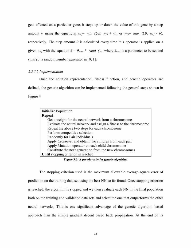
44
gets effected on a particular gene, it steps up or down the value of this gene by a step
amount θ using the equations wi,j= min (UB, wi,j + θ), or wi,j= max (LB, wi,j - θ),
respectively. The step amount θ is calculated every time this operator is applied on a
given wi,j with the equation θ = θmax * rand ( ), where θmax is a parameter to be set and
rand ( ) is random number generator in [0, 1].
3.2.5.2 Implementation
Once the solution representation, fitness function, and genetic operators are
defined, the genetic algorithm can be implemented following the general steps shown in
Figure 4.
Figure 3.6: A pseudo-code for genetic algorithm
The stopping criterion used is the maximum allowable average square error of
prediction on the training data set using the best NN so far found. Once stopping criterion
is reached, the algorithm is stopped and we then evaluate each NN in the final population
both on the training and validation data sets and select the one that outperforms the other
neural networks. This is one significant advantage of the genetic algorithm based
approach than the simple gradient decent based back propagation. At the end of its
Initialize Population
Repeat
Get a weight for the neural network from a chromosome
Evaluate the neural network and assign a fitness to the chromosome
Repeat the above two steps for each chromosome
Perform competitive selection
Randomly for Pair Individuals
Apply Crossover and obtain two children from each pair
Apply Mutation operator on each child chromosome
Constitute the next generation from the new chromosomes
Until stopping criterion is reached

45
iteration, the genetic algorithm approach can provide several thousands of neural
networks from which the one that provides a good prediction not only on the training data
set but also on the validation can be chosen.
The procedure in initializing the models is complete. It is important to understand
the advantages and the disadvantages of using non-parametric NN CERs versus CERs
based upon parametric.
3.2.5.3 Parametric versus Non-Parametric CERs
There are several advantages and disadvantages of using NNs as compared to
parametric models for CERs. The findings of Tu (1996) in comparing the two
methodologies are as follows:
Advantages of NN
1. Less statistical training required
2. Ability to detect complex nonlinear relationships between variables
3. Can detect all possible interactions between the predictor variables
4. Many forms of training algorithms
Disadvantages of NN
1. Calculations are in a “black box” thus limited ability to explicitly identify causal
relationships.
2. Neural networks models may be more difficult to apply in a particular field.
3. Require great computational resources
4. Are prone to over-fitting.
5. As the model development is empirical, relatively limited research with possibly
many methodological issues remaining

46
3.3 Data Envelopment Analysis
In recent times, data envelopment analysis (DEA), which was introduced by
Charnes et al. (1978), has become a popular management tool. It is commonly used to
rank the efficiency of products; one example is in the electrical (utilities) sector, in which
the government can compare different suppliers (Berg, 2010). As the models output the
efficiency, the efficiency, in turn, can be used to predict the target cost. Depending on the
application, the target cost can be extrapolated from the best, worst, or average
efficiency.
DEA is a mathematical technique used to measure the relative efficiency of
homogeneous decision-making units (DMUs) with multiple inputs and outputs. It is
applied when there is no obvious unit price information for some or all of the inputs and
the outputs to aggregate them into a single equivalent input and a single equivalent
output, respectively. In DEA, the relative efficiency of a DMU is defined as the ratio of
total weighted output to total weighted input. By considering a set of homogeneous N
decision making units (DMUn for n = 1, 2, · · ·, N) each having I number of inputs (xi,n for
i = 1, · · · , I), and O number of outputs (yo,n for o = 1, · · ·, O), the efficiency measure Ek
for DMUk is given by Equation (34), where the weights ui,k and vo,k are non-negative and
unknown until they are determined by the DEA procedure.
(36)
The weights ui,k and vo,k corresponding to DMUk are determined in such a way
that the efficiency Ek of this decision making unit can be maximized subject to the
(34)
1
,,
1
,,
O
o
kiki
O
o
koko
k
xv
yu
E

47
following constraints. The first one is, when these weights are applied to all DMUs they
should not provide any DMU with efficiency greater than one. The second one requires
the weights to be non-negative. This problem can be formulated for DMUk as fractional
linear programming mathematical model as follows.
Maximize:
(37)
Subject to:
(38)
(39)
DMUk will choose weights ui,k and vo,k so as to maximize its efficiency, given the
constraints in Equations (38) and (39). The fractional linear programming described
above can be transformed into a simple linear programming by multiplying both the
numerators and denominators of the fractions with a positive constant c and choosing the
constant c such that the following holds; ∑ The products of the
constant c and the variables ui,k and vo,k can be replaced by new variables pi,k and qo,k,
respectively. The resulting linear programming is shown below.
Maximize:
(40)
(35)
1
,,
1
,,
O
o
kiki
O
o
koko
k
xu
yv
E
(36) 1;
1
,,
1
,,
n
xu
yv
O
o
niki
O
o
noko
(37) , ; 0 , iovu o,ki,k
(38) 1
,,
O
o
kokok yqE
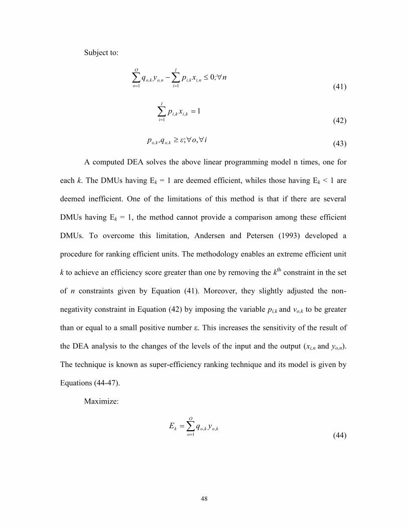
48
Subject to:
(41)
(42)
(43)
A computed DEA solves the above linear programming model n times, one for
each k. The DMUs having Ek = 1 are deemed efficient, whiles those having Ek < 1 are
deemed inefficient. One of the limitations of this method is that if there are several
DMUs having Ek = 1, the method cannot provide a comparison among these efficient
DMUs. To overcome this limitation, Andersen and Petersen (1993) developed a
procedure for ranking efficient units. The methodology enables an extreme efficient unit
k to achieve an efficiency score greater than one by removing the kth
constraint in the set
of n constraints given by Equation (41). Moreover, they slightly adjusted the non-
negativity constraint in Equation (42) by imposing the variable pi,k and vo,k to be greater
than or equal to a small positive number ε. This increases the sensitivity of the result of
the DEA analysis to the changes of the levels of the input and the output (xi,n and yo,n).
The technique is known as super-efficiency ranking technique and its model is given by
Equations (44-47).
Maximize:
(44)
(39)011
n;xpyqI
i
i,ni,k
O
o
o,no,k
(40) 11
,,
I
i
kiki xp
(41) ,; ioε,qp o,ko,k
(42) 1
,,
O
o
kokok yqE
49
Subject to:
(45)
(46)
(47)
This model is used as the basis for the study on cost estimation.
3.3.1 Advantages and Disadvantages of DEA
Upon studying the research of Berg and Lin (2008), Berg (2010), and Harton
(2011), the following strengths and weaknesses were identified.
Advantages of DEA
1. Mathematical function does need to be explicitly specified.
2. Discovers relationships that are limited in other methodologies.
3. Able to compute analyses with several inputs and output variables.
4. Easy to apply with any input – output measurement.
5. Inefficiency can be analyzed and quantified for every evaluated unit.
Disadvantages of DEA
1. Results are sensitive to the selection of inputs and output variables.
2. Limited application
3. Number of efficient samples tends to increase as the number of inputs and output
variables increase.
(43)011
k nn ;xpyqI
i
i,ni,k
O
o
o,no,k
(44) 11
,,
I
i
kiki xp
(45) ,; ioε,qp o,ko,k

50
3.4 Chapter Summary
This chapter presents the target cost models or the cost estimating relationships
(CERs) developed in this thesis. The first two models presented are based upon
regression. The next models presented are neural network models trained using back-
propagation and the genetic algorithm. Finally, the chapter concludes by presenting the
data envelopment analysis models developed and applied in the case. The case study is
presented in the following chapter.

51
4. Case Study at Bombardier Aerospace
The models developed in this thesis were applied at a case study conducted at a
major aerospace company. Bombardier Aerospace (BA) is a unit of Bombardier Inc. and
its headquarters are in Montreal, Quebec. Bombardier specializes in the design and
manufacture of innovative aviation products. Bombardier has about 30,000 employees
worldwide. Their large work force coupled with their annual revenues of over $8 Billion
dollars (BA 2011 Annual Report, 2012) highlight their significance to the Canadian
economy.
Bombardier has a large portfolio of business and regional jets. Their products in
business jets include the Challenger, Global Express, and Lear jet. The commercial jets
include the CRJs, Q-series, and they will soon be introducing the C-Series on the market.
Despite their achievements, they, like other aerospace companies, are facing many
challenges.
The extreme volatility of the fuel price in recent years has played an integral role
in their current financial difficulties. Moreover the competition is fierce; other airframes
such as Embraer are developing products in direct competition with BA. To makes
matters even more difficult other countries such as India and China are developing their
own aircrafts with subsidies from their respective governments.
Lin Ai, economist at the Conference Board of Canada states “The Canadian
aerospace industry must continue to improve the quality of its products and to develop
leading technology if it is to compete more effectively in the global marketplace”
(Conference Board of Canada, 2012). Bombardier is well aware of this predicament, and

52
they are constantly seeking to develop new programs, such as the C-Series and the Global
5000, in order to remain competitive and to gain new market segments.
Due to the economic situation at the time of this study, the emergence of cost
understanding initiatives had become critical, even at an early conceptual stage. Having
an accurate understanding of the cost of a new program was among the company‟s main
priorities. Crucial to the supply chain was to accurately predict a target cost for all major
structures and commodities in order to launch a new aircraft program, especially since
some of these commodities cost several millions of dollars. The models developed in this
thesis were therefore applied to BA to predict the target cost to help BA in bidding,
forecasting and strategic initiatives. This chapter will present the steps undertaken to
apply the cost model. It will discuss the data collection process, the product studied in
this case, and the identification of its cost drivers.
4.1 Data Collection
According to ISPA (2009), the sources of data can be primary, secondary, or both.
The primary data are derived from basic accounting records. The secondary data can be
extracted from contracts and cost proposals. Finally, the data that is classified as either
primary or secondary is cost reports, historical and technical databases, specialists, and
other information systems. In this study data was collected for 13 programs from the
following sources: technical databases, design drawings, specialists, historical databases,
contracts, extrapolation of data from the contracts, estimates based upon experts inputs,
and attendance at workshops. These sources of data helped to identify the commodity to
study, the cost drivers of that commodity, and collect pertinent details about the cost
drivers required for the model. Interviews were conducted and attendance at team

53
meetings helped to substantiate and validate some of the data collected. Challenges
specific to data collection are highlighted in the sections that follow.
4.1.1 Landing Gear
During the time of this study, research was already underway at BA to develop
models to determine target costs. Several commodities had already been identified for
study. The first commodity selected was the landing gear (LG). The LG, also known as
the undercarriage, is utilized as an interface between the aircraft and the ground. The
landing gear can be divided into different sub-systems such as: main landing gear (MLG),
nose landing gear (NLG), extension and retraction system, alternate release system,
steering system and brake control system. The main functions of the landing gear are to
absorb loads upon landing, taxiing and braking. The load during landing is absorbed by
the gears and it is proportional to the maximum takeoff weight (MTOW). The MTOW,
typically measured in pounds, is the heaviest weight at which the aircraft can takeoff and
fly and meets all the applicable airworthiness requirements. Figure 4.1 below shows an
MLG.
Figure 4.1: Lockheed C-5A MLG (Currey, 1988)

54
In this research, target cost models were applied to the MLGs based upon a select number
of cost drivers.
4.1.2 Cost Drivers
Lean accounting focuses on the product, its characteristics, and the customer
(Maskell and Baggaley, 2002). The characteristics of the products are the design
parameters, which will be used to formulate the cost model or the cost estimating relation
(CER). The design parameters that influence the cost of the product are the cost drivers.
Recalling Equation (3): CER (y) = f(xi), it can be seen that the cost drivers, xi are those
variables that will determine the cost of the product. Thus, selecting the right cost drivers
are of upmost importance.
As some of the design parameters can be the cost drivers, the technical specialists
responsible for the design of the aircraft were used as the primary source for establishing
the cost drivers. The cost drivers were selected through interviews with the technical
specialists in the advanced design team (ADT). The ADT is responsible for the
configuration and design of the aircraft from the conceptual phase of the design process.
They design the aircraft to meet the needs of the market, and the customer.
At a conceptual phase of design, only a few characteristics of the aircraft such as
the range, required thrust, maximum take-off weight (MTOW) are known. As the
selected product was the landing gear, and the aircraft had a defined MTOW, the
engineers had some characteristics about the component. Of the known characteristics,
upon extensive interviews, the following three design parameters were selected as the
cost drivers.
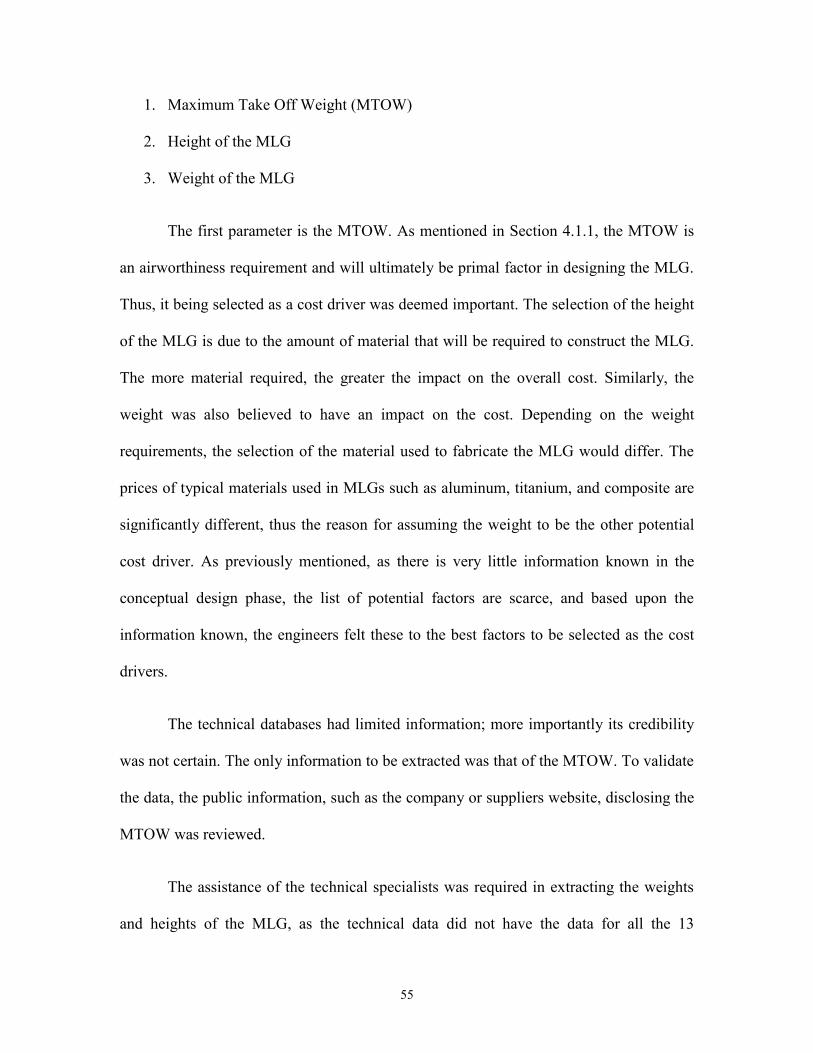
55
1. Maximum Take Off Weight (MTOW)
2. Height of the MLG
3. Weight of the MLG
The first parameter is the MTOW. As mentioned in Section 4.1.1, the MTOW is
an airworthiness requirement and will ultimately be primal factor in designing the MLG.
Thus, it being selected as a cost driver was deemed important. The selection of the height
of the MLG is due to the amount of material that will be required to construct the MLG.
The more material required, the greater the impact on the overall cost. Similarly, the
weight was also believed to have an impact on the cost. Depending on the weight
requirements, the selection of the material used to fabricate the MLG would differ. The
prices of typical materials used in MLGs such as aluminum, titanium, and composite are
significantly different, thus the reason for assuming the weight to be the other potential
cost driver. As previously mentioned, as there is very little information known in the
conceptual design phase, the list of potential factors are scarce, and based upon the
information known, the engineers felt these to the best factors to be selected as the cost
drivers.
The technical databases had limited information; more importantly its credibility
was not certain. The only information to be extracted was that of the MTOW. To validate
the data, the public information, such as the company or suppliers website, disclosing the
MTOW was reviewed.
The assistance of the technical specialists was required in extracting the weights
and heights of the MLG, as the technical data did not have the data for all the 13

56
programs considered to develop the cost models. The information was gathered in the
form of workshops. During the workshops, the computer aided design (CAD) drawings
were reviewed. From the drawings, the heights of the programs were extracted.
Moreover, the specialists were also able to extract the weight based upon the material and
volume of the MLG. However, in some cases there were no CAD drawings, due to legacy
systems, and only technical drawings available. For those programs, much effort was put
in reviewing the drawings, and estimating the weights, once again, based upon their
weights and their volume.
The cost data of the historical programs were extracted from the historical
databases and cross validated with the contracts. The reason for cross validating the
contract was mainly due to the manner in which the cost was stored in the database. In
some instances the database did not have the cost of the MLG but of the entire landing
gear (LG). In those cases the cost had to be extracted from the contracts. However the
contracts are not real time and are a static picture of the agreed upon price at contract
signature. As the contracts were for many years, a price adjustment formula was used as a
mechanism to adjust the price, typically upon an annual basis. Therefore, the cost of the
MLG would have to be extrapolated to the year of study.
Finally in one of the cases, the cost of the MLG was not broken down in the
contract as well. Therefore based upon inputs from experts and the comparison of the
cost structure other LGs, the cost of one MLG was estimated.

57
4.2 Chapter Summary
In this chapter, the case company in which the target cost models were applied,
Bombardier Aerospace is introduced. Thereafter, the particular commodity selected for
study is described. Next, the manner in which the selected cost drivers is discussed.
Finally, the steps followed to gather the data are outlined. The results and analysis are
presented in the following chapter.
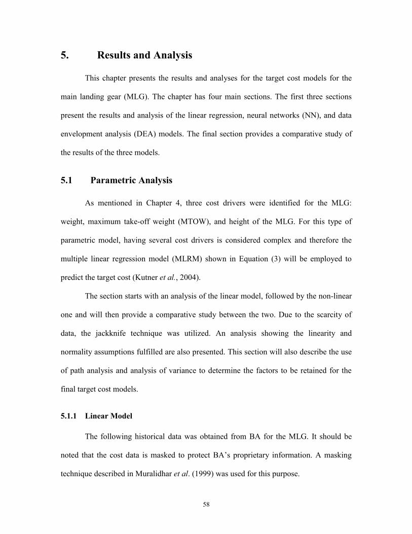
58
5. Results and Analysis
This chapter presents the results and analyses for the target cost models for the
main landing gear (MLG). The chapter has four main sections. The first three sections
present the results and analysis of the linear regression, neural networks (NN), and data
envelopment analysis (DEA) models. The final section provides a comparative study of
the results of the three models.
5.1 Parametric Analysis
As mentioned in Chapter 4, three cost drivers were identified for the MLG:
weight, maximum take-off weight (MTOW), and height of the MLG. For this type of
parametric model, having several cost drivers is considered complex and therefore the
multiple linear regression model (MLRM) shown in Equation (3) will be employed to
predict the target cost (Kutner et al., 2004).
The section starts with an analysis of the linear model, followed by the non-linear
one and will then provide a comparative study between the two. Due to the scarcity of
data, the jackknife technique was utilized. An analysis showing the linearity and
normality assumptions fulfilled are also presented. This section will also describe the use
of path analysis and analysis of variance to determine the factors to be retained for the
final target cost models.
5.1.1 Linear Model
The following historical data was obtained from BA for the MLG. It should be
noted that the cost data is masked to protect BA‟s proprietary information. A masking
technique described in Muralidhar et al. (1999) was used for this purpose.
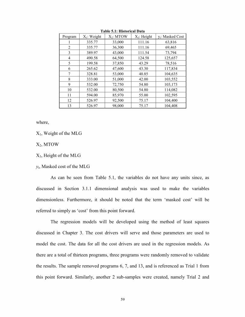
59
Table 5.1: Historical Data
Program X1: Weight X2: MTOW X3: Height yi: Masked Cost
1 335.77 33,000 111.16 63,816
2 335.77 36,300 111.16 69,465
3 389.97 43,000 111.54 73,794
4 490.58 64,500 124.58 125,657
5 199.58 37,850 43.29 78,516
6 265.62 47,600 43.30 117,834
7 328.81 53,000 40.85 104,635
8 333.00 51,000 42.00 103,552
9 532.00 72,750 54.80 103,173
10 532.00 80,500 54.80 114,082
11 594.00 85,970 55.00 102,595
12 526.97 92,500 75.17 104,400
13 526.97 98,000 75.17 104,408
where,
X1, Weight of the MLG
X2, MTOW
X3, Height of the MLG
yi, Masked cost of the MLG
As can be seen from Table 5.1, the variables do not have any units since, as
discussed in Section 3.1.1 dimensional analysis was used to make the variables
dimensionless. Furthermore, it should be noted that the term „masked cost‟ will be
referred to simply as „cost‟ from this point forward.
The regression models will be developed using the method of least squares
discussed in Chapter 3. The cost drivers will serve and those parameters are used to
model the cost. The data for all the cost drivers are used in the regression models. As
there are a total of thirteen programs, three programs were randomly removed to validate
the results. The sample removed programs 6, 7, and 13, and is referenced as Trial 1 from
this point forward. Similarly, another 2 sub-samples were created, namely Trial 2 and

60
Trial 3. Trial 2 omitted programs 2, 8, and 12, whereas Trial 3 omitted programs 3, 7, and
9. As previously mentioned, due to the limited data, the jackknife technique is utilized.
As required by the jackknife method, a regression analysis was conducted for
each sub sample. The following table summarizes the resulting equations from the
regression analysis of Trial 1 without the jackknife technique (y3) and for each sub-
sample utilizing jackknife (y3A-J, where the subscripts A to J refer to the sample in
question).
Table 5.2: Summary of LG jackknife equations for 3 factors
Recall that in Section 3.1.2, the linearity and normality assumptions must be
fulfilled. The following set of figures (Figures 5.1 - 5.10), are the SPC charts were used
validate the fulfillment of the linearity assumption. Furthermore, it should be recalled
from Section 3.1.2.1, the control limits are ±3ζ of the residuals.

61
Figure 5.1: SPC chart for LR, 3 factors, sample A
Figure 5.2: SPC chart for LR, 3 factors, sample B
60000
70000
80000
90000
100000
110000
120000
130000
60000 70000 80000 90000 100000 110000 120000 130000
Mas
ked
Co
st
Target Cost
60000
70000
80000
90000
100000
110000
120000
130000
60000 70000 80000 90000 100000 110000 120000 130000
Mas
ked
Co
st
Target Cost
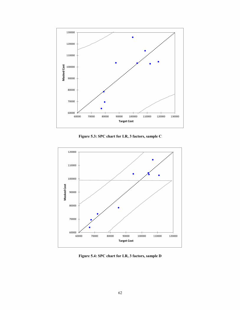
62
Figure 5.3: SPC chart for LR, 3 factors, sample C
Figure 5.4: SPC chart for LR, 3 factors, sample D
60000
70000
80000
90000
100000
110000
120000
130000
60000 70000 80000 90000 100000 110000 120000 130000
Mas
ked
Co
st
Target Cost
60000
70000
80000
90000
100000
110000
120000
60000 70000 80000 90000 100000 110000 120000
Mas
ked
Co
st
Target Cost

63
Figure 5.5: SPC chart for LR, 3 factors, sample E
Figure 5.6: SPC chart for LR, 3 factors, sample F
60000
70000
80000
90000
100000
110000
120000
130000
60000 70000 80000 90000 100000 110000 120000 130000
Mas
ked
Co
st
Target Cost
60000
70000
80000
90000
100000
110000
120000
130000
60000 70000 80000 90000 100000 110000 120000 130000
Mas
ked
Co
st
Target Cost
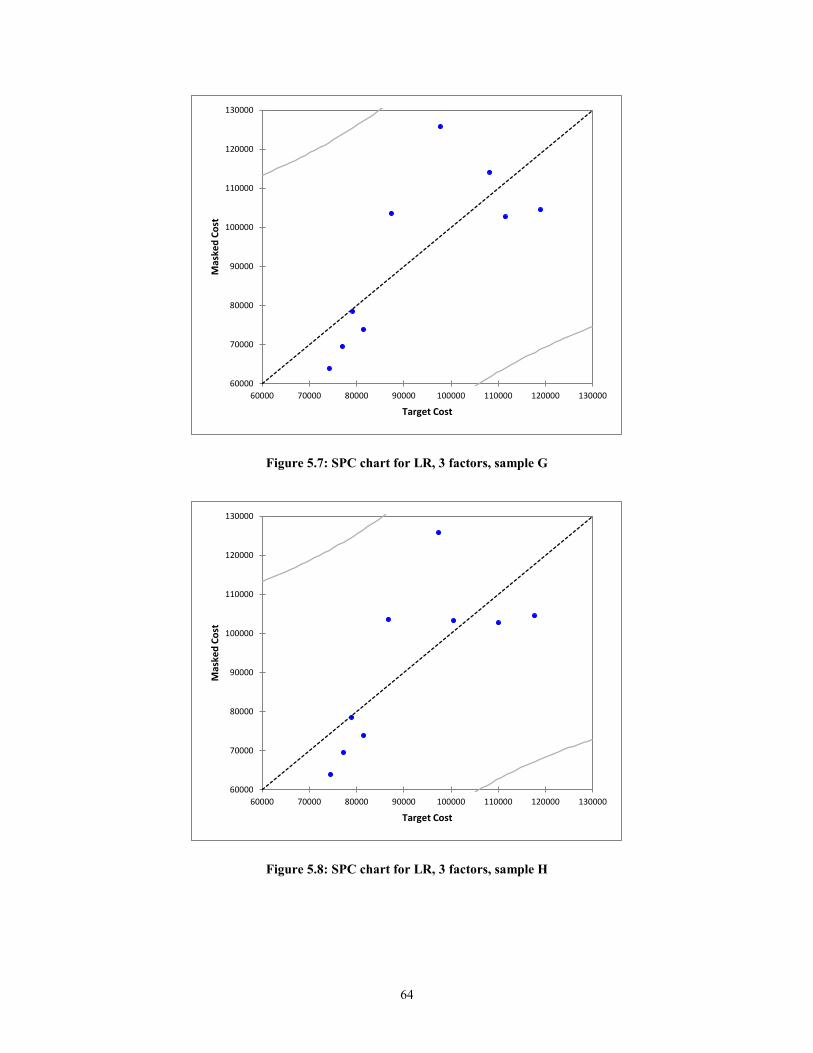
64
Figure 5.7: SPC chart for LR, 3 factors, sample G
Figure 5.8: SPC chart for LR, 3 factors, sample H
60000
70000
80000
90000
100000
110000
120000
130000
60000 70000 80000 90000 100000 110000 120000 130000
Mas
ked
Co
st
Target Cost
60000
70000
80000
90000
100000
110000
120000
130000
60000 70000 80000 90000 100000 110000 120000 130000
Mas
ked
Co
st
Target Cost
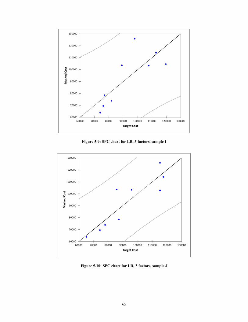
65
Figure 5.9: SPC chart for LR, 3 factors, sample I
Figure 5.10: SPC chart for LR, 3 factors, sample J
60000
70000
80000
90000
100000
110000
120000
130000
60000 70000 80000 90000 100000 110000 120000 130000
Mas
ked
Co
st
Target Cost
60000
70000
80000
90000
100000
110000
120000
130000
60000 70000 80000 90000 100000 110000 120000 130000
Mas
ked
Co
st
Target Cost
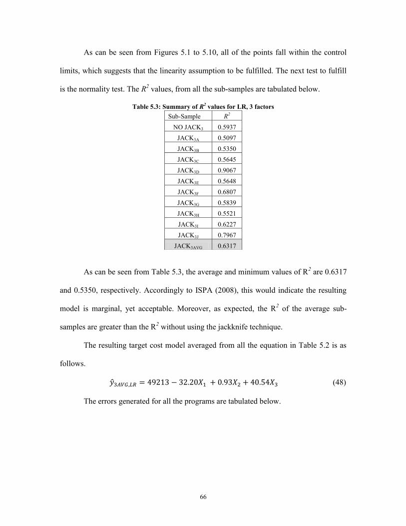
66
As can be seen from Figures 5.1 to 5.10, all of the points fall within the control
limits, which suggests that the linearity assumption to be fulfilled. The next test to fulfill
is the normality test. The R2 values, from all the sub-samples are tabulated below.
Table 5.3: Summary of R2 values for LR, 3 factors
As can be seen from Table 5.3, the average and minimum values of R2 are 0.6317
and 0.5350, respectively. Accordingly to ISPA (2008), this would indicate the resulting
model is marginal, yet acceptable. Moreover, as expected, the R2 of the average sub-
samples are greater than the R2 without using the jackknife technique.
The resulting target cost model averaged from all the equation in Table 5.2 is as
follows.
(48)
The errors generated for all the programs are tabulated below.
Sub-Sample R2
NO JACK3 0.5937
JACK3A 0.5097
JACK3B 0.5350
JACK3C 0.5645
JACK3D 0.9067
JACK3E 0.5648
JACK3F 0.6807
JACK3G 0.5839
JACK3H 0.5521
JACK3I 0.6227
JACK3J 0.7967
JACK3AVG 0.6317
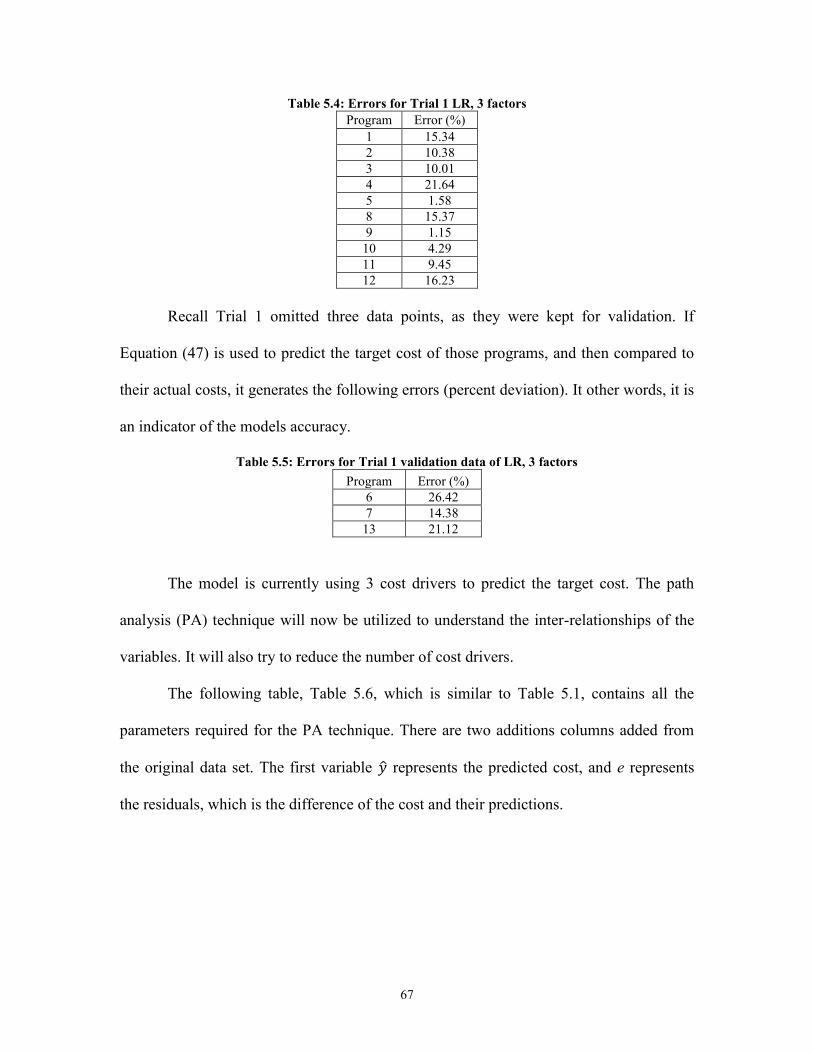
67
Table 5.4: Errors for Trial 1 LR, 3 factors
Program Error (%)
1 15.34
2 10.38
3 10.01
4 21.64
5 1.58
8 15.37
9 1.15
10 4.29
11 9.45
12 16.23
Recall Trial 1 omitted three data points, as they were kept for validation. If
Equation (47) is used to predict the target cost of those programs, and then compared to
their actual costs, it generates the following errors (percent deviation). It other words, it is
an indicator of the models accuracy.
Table 5.5: Errors for Trial 1 validation data of LR, 3 factors
Program Error (%)
6 26.42
7 14.38
13 21.12
The model is currently using 3 cost drivers to predict the target cost. The path
analysis (PA) technique will now be utilized to understand the inter-relationships of the
variables. It will also try to reduce the number of cost drivers.
The following table, Table 5.6, which is similar to Table 5.1, contains all the
parameters required for the PA technique. There are two additions columns added from
the original data set. The first variable represents the predicted cost, and e represents
the residuals, which is the difference of the cost and their predictions.

68
Table 5.6: Data for PA in LR, 3 factors
N x1 x2 x3 y e
1 335.77 33,000 111.16 63,816 74,327 -10,511
2 335.77 36,300 111.16 69,465 77,009 -7,544
3 389.97 43,000 111.54 73,794 81,579 -7,785
4 490.58 64,500 124.58 125,657 97,676 27,981
5 199.58 37,850 43.29 78,516 79,110 -594
8 333.00 51,000 42 103,552 87,599 15,953
9 532.00 72,750 54.8 103,173 102,294 879
10 532.00 80,500 54.8 114,082 108,591 5,491
11 594.00 85,970 55 102,595 112,031 -9,436
12 526.97 92,500 75.17 104,400 118,835 -14,435
ζ2 15,839 498,263,801 1,067 435,984,173 258,856,698 177,127,475
ζ 125.85 22,322 32.66 20880 16089 13309
It should be noted, that Table 5.6, contains the results without the jackknife
technique. As the jackknife technique is used to reduce the bias, the underlying inter-
relations of the cost and their drivers are derived from the data without using the
jackknife technique.
Table 5.7: Correlation matrix LR
x2 x3 Y
x1 0.890 -0.055 0.673
x2 -0.367 0.770
x3 -0.282
From Equations (20) and (21), the path coefficients would be calculated as the following.
Table 5.8: Path coefficients for LR, 3 factors
Path Coefficients Value
p01 -0.0980
p02 0.8686
p03 0.0317
p0U 0.6374
The resulting PA diagram is shown in Figure 5.11.

69
Figure 5.11: PA for LR, 3 factors
As can be seen in the diagram the effects of each of the cost drivers have on the
cost is shown. The higher the value of the arrow connecting the cost drivers to the cost, in
order words the path coefficient, the more importance it will have in determining the cost.
In this diagram, it is clearly shown that the cost driver that most influences the cost, is the
MTOW.
Moreover, the arrows connecting the cost drivers to one another are the
correlations. In other words, it shows the degree of dependency the cost drivers have one
another. It also represents the direct of the relationship. For example, in this instance as
the correlation between the MTOW and the weight is positive, it would indicate that as
the MTOW would increase, the weight would also follow. Finally, the variable U
represents the value of the cost function not being represented by its drivers. The lower
the value, the greater the cost drivers represent the cost.
In order to minimize the number of cost drivers, the procedure stipulated in
Section 3.1.4.1 is followed. By utilizing Equation (26) and by cross validating with
Equation (27), to calculate the coefficient of determination, R2, the following result are
obtained.
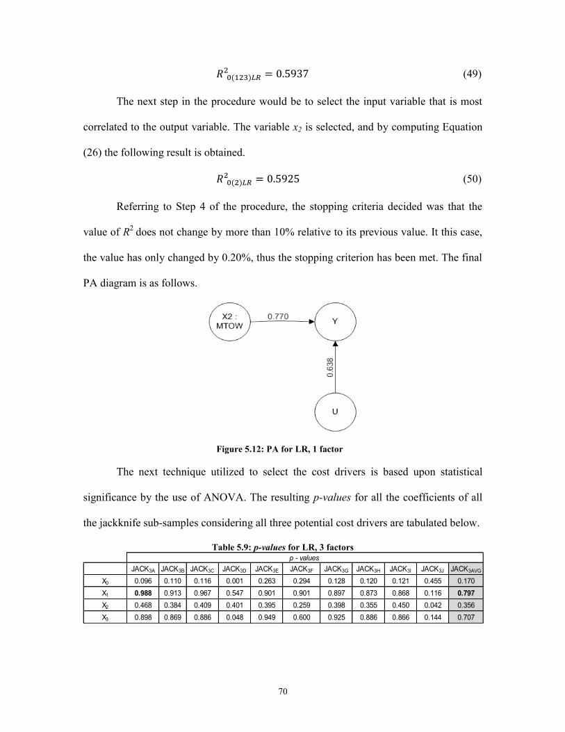
70
(49)
The next step in the procedure would be to select the input variable that is most
correlated to the output variable. The variable x2 is selected, and by computing Equation
(26) the following result is obtained.
(50)
Referring to Step 4 of the procedure, the stopping criteria decided was that the
value of R2
does not change by more than 10% relative to its previous value. It this case,
the value has only changed by 0.20%, thus the stopping criterion has been met. The final
PA diagram is as follows.
Figure 5.12: PA for LR, 1 factor
The next technique utilized to select the cost drivers is based upon statistical
significance by the use of ANOVA. The resulting p-values for all the coefficients of all
the jackknife sub-samples considering all three potential cost drivers are tabulated below.
Table 5.9: p-values for LR, 3 factors
JACK3A JACK3B JACK3C JACK3D JACK3E JACK3F JACK3G JACK3H JACK3I JACK3J JACK3AVG
X0 0.096 0.110 0.116 0.001 0.263 0.294 0.128 0.120 0.121 0.455 0.170
X1 0.988 0.913 0.967 0.547 0.901 0.901 0.897 0.873 0.868 0.116 0.797
X2 0.468 0.384 0.409 0.401 0.395 0.259 0.398 0.355 0.450 0.042 0.356
X3 0.898 0.869 0.886 0.048 0.949 0.600 0.925 0.886 0.866 0.144 0.707
p - values
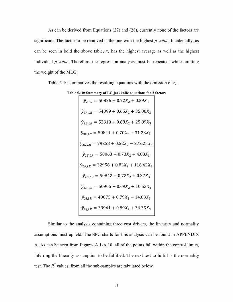
71
As can be derived from Equations (27) and (28), currently none of the factors are
significant. The factor to be removed is the one with the highest p-value. Incidentally, as
can be seen in bold the above table, x1 has the highest average as well as the highest
individual p-value. Therefore, the regression analysis must be repeated, while omitting
the weight of the MLG.
Table 5.10 summarizes the resulting equations with the omission of x1.
Table 5.10: Summary of LG jackknife equations for 2 factors
Similar to the analysis containing three cost drivers, the linearity and normality
assumptions must upheld. The SPC charts for this analysis can be found in APPENDIX
A. As can be seen from Figures A.1-A.10, all of the points fall within the control limits,
inferring the linearity assumption to be fulfilled. The next test to fulfill is the normality
test. The R2 values, from all the sub-samples are tabulated below.

72
Table 5.11: Summary of R2 values for LR, 2 factors
Sub-Sample R2
NO JACK2,LR 0.5925
JACK2A,LR 0.5097
JACK2B,LR 0.5338
JACK2C,LR 0.5643
JACK2D,LR 0.8989
JACK2E,LR 0.5633
JACK2F,LR 0.6795
JACK2G,LR 0.5824
JACK2H,LR 0.5495
JACK2I,LR 0.6204
JACK2J,LR 0.6505
JACK2AVG 0.6152
As can be seen from Table 5.11, the average and minimum values of R2 are
0.6152 and 0.5097, respectively. Accordingly to ISPA (2009), this would indicate the
resulting model to be marginal, yet acceptable. The resulting equation (target cost model)
from the jackknife equations in Table 5.11 is as follows.
(51)
The errors generated for all the programs are tabulated below.
Table 5.12: Errors for Trial 1 LR, 2 factors
Program Error (%)
1 16.8
2 10.7
3 10.7
4 22.7
5 0.4
8 15.4
9 0.1
10 4.6
11 9.9
12 12.5
By computing Equation (50) predict the target cost of the validation programs,
and then compared to their actual costs, it would generate the following errors (percent
deviation).
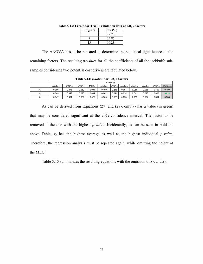
73
Table 5.13: Errors for Trial 1 validation data of LR, 2 factors
Program Error (%)
6 27.70
7 14.86
13 16.28
The ANOVA has to be repeated to determine the statistical significance of the
remaining factors. The resulting p-values for all the coefficients of all the jackknife sub-
samples considering two potential cost drivers are tabulated below.
Table 5.14: p-values for LR, 2 factors
As can be derived from Equations (27) and (28), only x2 has a value (in green)
that may be considered significant at the 90% confidence interval. The factor to be
removed is the one with the highest p-value. Incidentally, as can be seen in bold the
above Table, x3 has the highest average as well as the highest individual p-value.
Therefore, the regression analysis must be repeated again, while omitting the height of
the MLG.
Table 5.15 summarizes the resulting equations with the omission of x1, and x3.
JACK2A JACK2B JACK2C JACK2D JACK2E JACK2F JACK2G JACK2H JACK2I JACK2J JACK2AVG
X0 0.066 0.078 0.082 0.001 0.190 0.246 0.091 0.086 0.088 0.160 0.109
X2 0.049 0.043 0.035 0.004 0.061 0.014 0.034 0.041 0.025 0.020 0.033
X3 0.847 0.891 0.869 0.025 0.983 0.538 0.998 0.955 0.934 0.834 0.788
p - values

74
Table 5.15: Summary of LG jackknife equations for 1 factor
The SPC charts for this analysis can be found in APPENDIX B. As can be seen
from Figures B.1 - B.10, all of the points fall within the control limits, inferring the
linearity assumption to be fulfilled. The next test to fulfill is the normality test. The R2
values, from all the sub-samples are tabulated below.
Table 5.16: Summary of R2 values for LR, 1 factor
Sample R2
NO JACK1,LR 0.5925
JACK1A,LR 0.5064
JACK1B,LR 0.5322
JACK1C,LR 0.5622
JACK1D,LR 0.7494
JACK1E,LR 0.5633
JACK1F,LR 0.6568
JACK1G,LR 0.5824
JACK1H,LR 0.5492
JACK1I,LR 0.6199
JACK1J,LR 0.6477
JACK1AVG,LR 0.5970
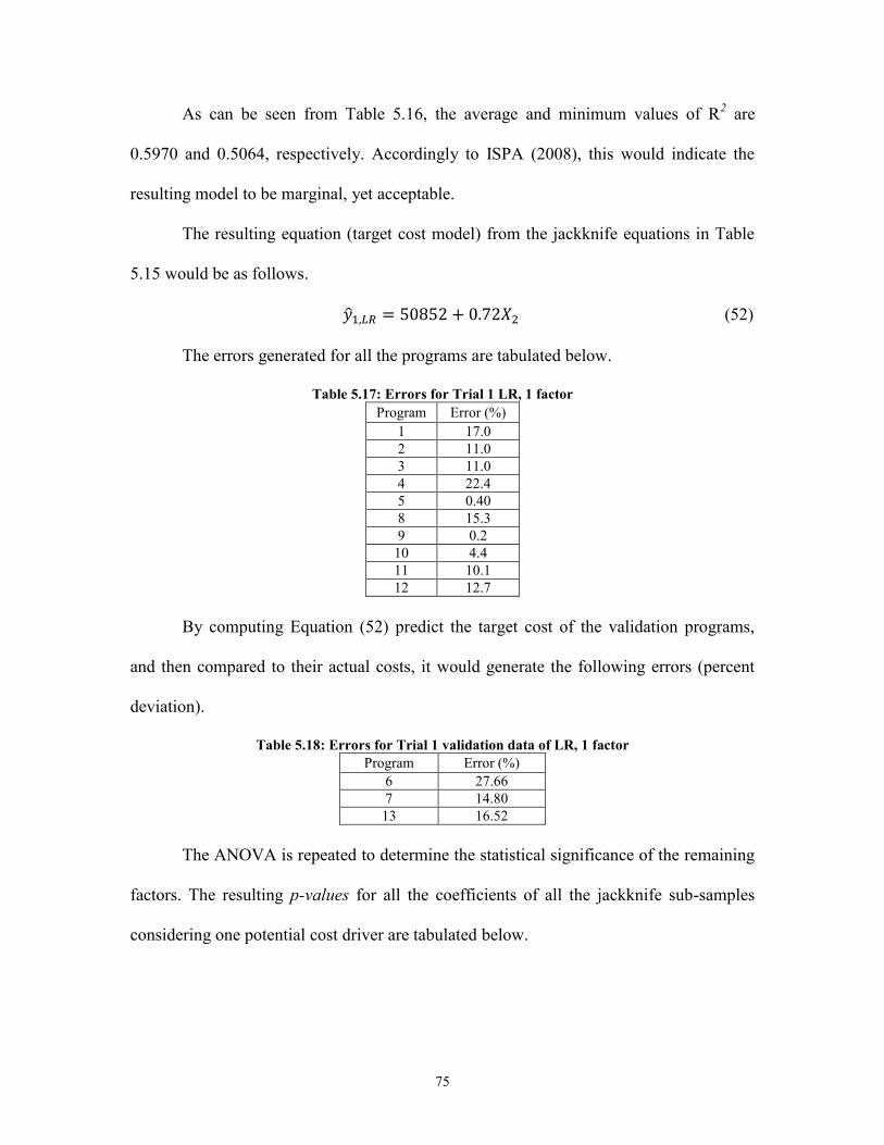
75
As can be seen from Table 5.16, the average and minimum values of R2 are
0.5970 and 0.5064, respectively. Accordingly to ISPA (2008), this would indicate the
resulting model to be marginal, yet acceptable.
The resulting equation (target cost model) from the jackknife equations in Table
5.15 would be as follows.
(52)
The errors generated for all the programs are tabulated below.
Table 5.17: Errors for Trial 1 LR, 1 factor
Program Error (%)
1 17.0
2 11.0
3 11.0
4 22.4
5 0.40
8 15.3
9 0.2
10 4.4
11 10.1
12 12.7
By computing Equation (52) predict the target cost of the validation programs,
and then compared to their actual costs, it would generate the following errors (percent
deviation).
Table 5.18: Errors for Trial 1 validation data of LR, 1 factor
Program Error (%)
6 27.66
7 14.80
13 16.52
The ANOVA is repeated to determine the statistical significance of the remaining
factors. The resulting p-values for all the coefficients of all the jackknife sub-samples
considering one potential cost driver are tabulated below.

76
Table 5.19: p-values for LR, 1 factor
As can be derived from Equations (27) and (28), both x0 and x2 have values (in
green) that may be considered significant at the 90% confidence interval.
The analysis for the LR is now complete. The model has collapsed on one
significant factor, x2 (MTOW). This is also the same finding for PA. The next analysis to
be conducted is to see how the results impact the non-linear target cost model.
5.1.2 Analysis Based on a Non-Linear Model
As discussed in Section 3.1, as the target cost will be in the form of Equation (4),
it will have to be transformed into a linear format (Equation 5) to conduct regression
analysis. In order to convert the data into proper form for the analysis, the natural log (ln)
will have to be taken for all input and output data. The transformed data can be seen in
Table 5.20.
Table 5.20: Historical Data (ln values)
Program ln x1 ln x2 ln x3 ln y
1 5.8164 10.4043 4.7110 11.0638
2 5.8164 10.4996 4.7110 11.1486
3 5.9661 10.6690 4.7144 11.2090
4 6.1956 11.0744 4.8249 11.7413
5 5.2962 10.5414 3.7679 11.2711
6 5.5821 10.7706 3.7682 11.6770
7 5.7955 10.8780 3.7099 11.5582
8 5.8081 10.8396 3.7377 11.5478
9 6.2766 11.1948 4.0037 11.5442
10 6.2766 11.2960 4.0037 11.6447
11 6.3869 11.3618 4.0073 11.5385
12 6.2671 11.4350 4.3198 11.5560
13 6.2671 11.4927 4.3198 11.5561
JACK1A JACK1B JACK1C JACK1D JACK1E JACK1F JACK1G JACK1H JACK1I JACK1J JACK1AVG
X0 0.008 0.010 0.008 0.001 0.015 0.010 0.009 0.009 0.013 0.013 0.009
X2 0.032 0.026 0.020 0.003 0.020 0.008 0.017 0.022 0.012 0.012 0.017
p - values

77
The methodology applied for the linear model will be applied. Trial 1 will be used
for the analysis, which will omit the programs 6, 7, and 13, as they will be kept for the
validation. Table 5.21 summarizes the resulting equations from the regression analysis of
Trial 1 without the jackknife technique and for each sub-sample utilizing jackknife.
Table 5.21: Summary of LG jackknife equations for 3 factors
The SPC charts, to fulfill the linearity assumptions are in APPENDIX C. As can
be seen from Figures C.1 –C.10 all of the values fall within the control limits implying
the model to be statistically linear.

78
The R2 values, to fulfill the normality test are as follows.
Table 5.22: Summary of R2 values for NLM, 3 factors
Sub-Sample R2
NO JACK3,NLM 0.7380
JACK3A,NLM 0.6442
JACK3B,NLM 0.6877
JACK3C,NLM 0.7180
JACK3D,NLM 0.9464
JACK3E,NLM 0.7382
JACK3F,NLM 0.8078
JACK3G,NLM 0.7296
JACK3H,NLM 0.7105
JACK3I,NLM 0.7545
JACK3J,NLM 0.8421
JACK3AVG,NLM 0.7579
As can be seen from Table 5.22, the average value of R2 is 0.7579. Accordingly to
ISPA (2008), this would indicate that the resulting model is good.
The resulting equation (target cost model) from all the equation in Table 5.21 is as
follows.
(53)
The errors generated from Equation (53) for all the programs in Trial 1 are
tabulated below.
Table 5.23: Errors for Trial 1 NLM, 3 factors
Program Error (%)
1 6.03
2 4.13
3 6.26
4 21.53
5 5.01
8 13.92
9 0.78
10 3.68
11 9.07
12 17.46

79
Using Equation (53) on the validation to predict the target cost of those programs,
and then comparing them to the actual costs generates the following errors (percent
deviation).
Table 5.24: Errors for Trial 1 validation data of NLM, 3 factors
Program Error (%)
6 23.60
7 12.28
13 22.29
The model is currently using 3 cost drivers to predict the target cost. The PA
technique will now be utilized to understand the inter-relationships of the variables. It
will also try to reduce the number of cost drivers.
The following Table, Table 5.25, which is similar to Table 5.20, contains all the
parameters required for the path analysis technique.
Table 5.25: Data for PA in NLM, 3 factors
n x1 x2 x3 y e
1 5.8164 10.4043 4.7110 11.0638 11.1251 -0.0613
2 5.8164 10.4996 4.7110 11.1486 11.1897 -0.0411
3 5.9661 10.6690 4.7144 11.2090 11.2713 -0.0623
4 6.1956 11.0744 4.8249 11.7413 11.4985 0.2428
5 5.2962 10.5414 3.7679 11.2711 11.3057 -0.0346
8 5.8081 10.8396 3.7377 11.5478 11.3929 0.1549
9 6.2766 11.1948 4.0037 11.5442 11.5374 0.0067
10 6.2766 11.2960 4.0037 11.6447 11.6061 0.0386
11 6.3869 11.3618 4.0073 11.5385 11.6262 -0.0877
12 6.2671 11.4350 4.3198 11.5560 11.7120 -0.1560
ζ2 0.1124 0.1506 0.1825 0.0539 0.0398 0.0141
ζ 0.3353 0.3881 0.4271 0.2321 0.1994 0.1188
Similar to the case of LR, Table 5.25 contains the results of the predicted cost and
their associated residuals, without utilizing the jackknife technique. If recalled from
Section 3.1, the covariance matrix (Table 5.26) will be used on the PA diagram, to map
out the inter-relationships between the variables.
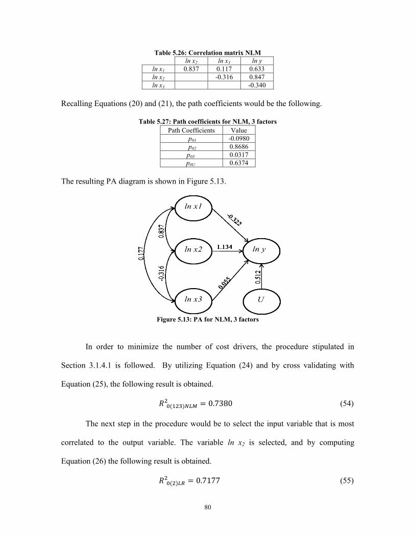
80
Table 5.26: Correlation matrix NLM
ln x2 ln x3 ln y
ln x1 0.837 0.117 0.633
ln x2 -0.316 0.847
ln x3 -0.340
Recalling Equations (20) and (21), the path coefficients would be the following.
Table 5.27: Path coefficients for NLM, 3 factors
Path Coefficients Value
p01 -0.0980
p02 0.8686
p03 0.0317
p0U 0.6374
The resulting PA diagram is shown in Figure 5.13.
Figure 5.13: PA for NLM, 3 factors
In order to minimize the number of cost drivers, the procedure stipulated in
Section 3.1.4.1 is followed. By utilizing Equation (24) and by cross validating with
Equation (25), the following result is obtained.
(54)
The next step in the procedure would be to select the input variable that is most
correlated to the output variable. The variable ln x2 is selected, and by computing
Equation (26) the following result is obtained.
(55)
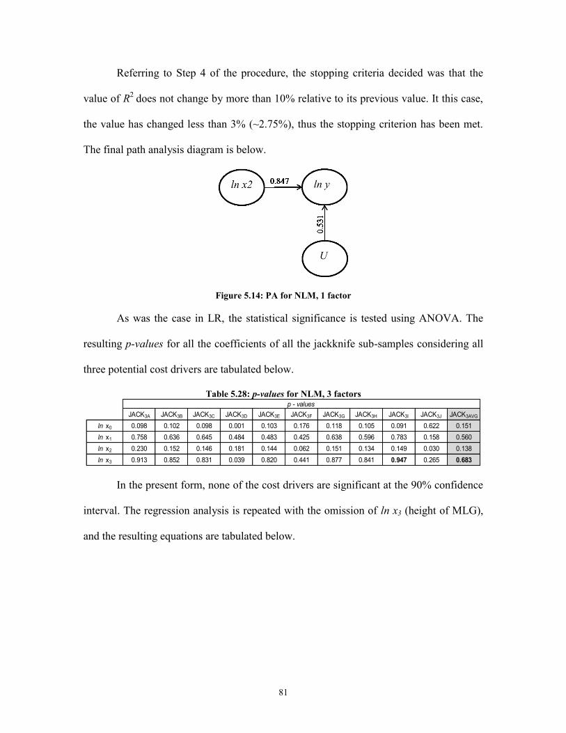
81
Referring to Step 4 of the procedure, the stopping criteria decided was that the
value of R2
does not change by more than 10% relative to its previous value. It this case,
the value has changed less than 3% (~2.75%), thus the stopping criterion has been met.
The final path analysis diagram is below.
Figure 5.14: PA for NLM, 1 factor
As was the case in LR, the statistical significance is tested using ANOVA. The
resulting p-values for all the coefficients of all the jackknife sub-samples considering all
three potential cost drivers are tabulated below.
Table 5.28: p-values for NLM, 3 factors
In the present form, none of the cost drivers are significant at the 90% confidence
interval. The regression analysis is repeated with the omission of ln x3 (height of MLG),
and the resulting equations are tabulated below.
JACK3A JACK3B JACK3C JACK3D JACK3E JACK3F JACK3G JACK3H JACK3I JACK3J JACK3AVG
ln x0 0.098 0.102 0.098 0.001 0.103 0.176 0.118 0.105 0.091 0.622 0.151
ln x1 0.758 0.636 0.645 0.484 0.483 0.425 0.638 0.596 0.783 0.158 0.560
ln x2 0.230 0.152 0.146 0.181 0.144 0.062 0.151 0.134 0.149 0.030 0.138
ln x3 0.913 0.852 0.831 0.039 0.820 0.441 0.877 0.841 0.947 0.265 0.683
p - values

82
Table 5.29: Summary of NLM jackknife equations for 2 factors
The SPC charts for the linearity test can be found in APPENDIX D. Figures D.1-D.10
infer the linearity constraint to be upheld as all the points are within the control limits.
The R2 values, for the normality test are as follows.
Table 5.30: Summary of R2 values for LR, 2 factors
Sub-Sample R2
NO JACK2,NLM 0.7368
JACK2A,NLM 0.6433
JACK2B,NLM 0.6853
JACK2C,NLM 0.7151
JACK2D,NLM 0.8631
JACK2E,NLM 0.7352
JACK2F,NLM 0.7809
JACK2G,NLM 0.7282
JACK2H,NLM 0.7079
JACK2I,NLM 0.7543
JACK2J,NLM 0.7924
JACK2AVG,NLM 0.7406

83
As the average values are above 0.70, the model is considered good (ISPA, 2008).
The resulting equation (target cost model) from the jackknife equations in Table 5.30
would be as follows.
(56)
The errors generated for all the programs are tabulated below.
Table 5.31: Errors for Trial 1 NLM, 2 factors
Program Error (%)
1 6.60
2 4.12
3 6.16
4 22.61
5 4.70
8 23.52
9 11.46
10 12.94
11 0.25
12 3.23
Table 5.32 gives the errors of the validation data.
Table 5.32: Errors for Trial 1 validation data of NLM, 2 factors
Program Error (%)
6 23.52
7 11.46
13 20.21
The ANOVA for the two remaining factors are as follows.
Table 5.33: p-values for NLM, 2 factors
From Table 5.33, it would indicate the insignificance of the weight of the MLG.
Thus, the analysis is repeated again with only the MTOW as the potential cost driver. The
resulting equations are as follows.
JACK3A JACK3B JACK3C JACK3D JACK3E JACK3F JACK3G JACK3H JACK3I JACK3J JACK3AVG
ln x0 0.013 0.012 0.009 0.001 0.008 0.005 0.009 0.010 0.012 0.020 0.010
ln x1 0.716 0.591 0.629 0.185 0.448 0.707 0.541 0.531 0.584 0.332 0.526
ln x2 0.093 0.052 0.049 0.004 0.062 0.030 0.033 0.036 0.025 0.013 0.040
p - values

84
Table 5.34: Summary of LG jackknife equations for 1 factor
The SPC charts found in APPENDIX E (Figures E1-E.10) infer the linearity
assumption to be fulfilled. The R2 values for the linearity test are as follows.
Table 5.35: Summary of R2 values for NLM, 1 factor
Sub-Sample R2
NO JACK1,NLM 0.7177
JACK1A,NLM 0.6347
JACK1B,NLM 0.6685
JACK1C,NLM 0.7028
JACK1D,NLM 0.8120
JACK1E,NLM 0.7061
JACK1F,NLM 0.7752
JACK1G,NLM 0.7091
JACK1H,NLM 0.6864
JACK1I,NLM 0.7406
JACK1J,NLM 0.7539
JACK11AVG,NLM 0.7189
As the average value is greater than 0.70, the model is acceptable.
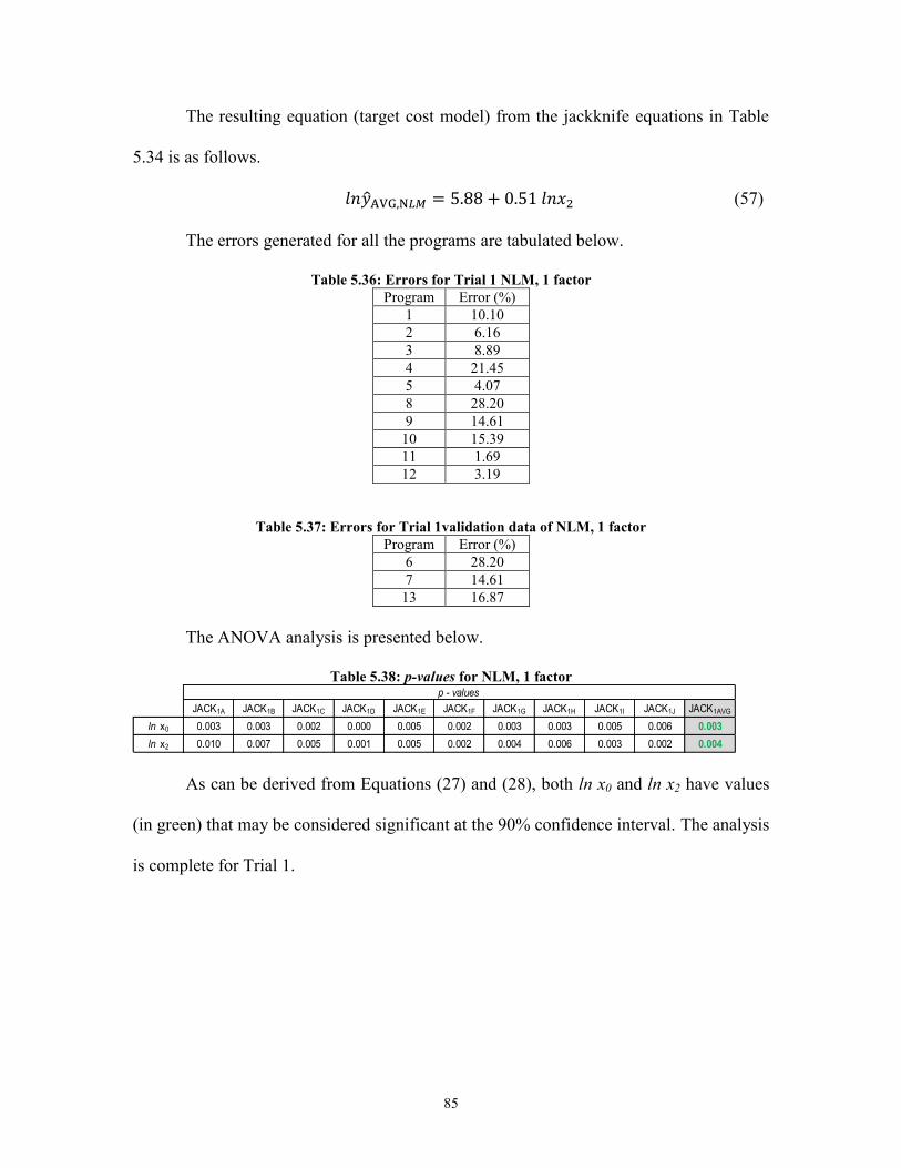
85
The resulting equation (target cost model) from the jackknife equations in Table
5.34 is as follows.
(57)
The errors generated for all the programs are tabulated below.
Table 5.36: Errors for Trial 1 NLM, 1 factor
Program Error (%)
1 10.10
2 6.16
3 8.89
4 21.45
5 4.07
8 28.20
9 14.61
10 15.39
11 1.69
12 3.19
Table 5.37: Errors for Trial 1validation data of NLM, 1 factor
Program Error (%)
6 28.20
7 14.61
13 16.87
The ANOVA analysis is presented below.
Table 5.38: p-values for NLM, 1 factor
As can be derived from Equations (27) and (28), both ln x0 and ln x2 have values
(in green) that may be considered significant at the 90% confidence interval. The analysis
is complete for Trial 1.
JACK1A JACK1B JACK1C JACK1D JACK1E JACK1F JACK1G JACK1H JACK1I JACK1J JACK1AVG
ln x0 0.003 0.003 0.002 0.000 0.005 0.002 0.003 0.003 0.005 0.006 0.003
ln x2 0.010 0.007 0.005 0.001 0.005 0.002 0.004 0.006 0.003 0.002 0.004
p - values

86
5.1.3 Analysis for Trials 2 and 3: Linear and Non-Linear Model
The analysis was repeated Trials 2 and 3. For both trials, the CERs were solely
using the MTOW as the significant cost driver. The errors for the LR and NLM are
presented below.
Table 5.39: Errors for Trial 2 LR, 1 factor
Program Error (%)
1 31.06
3 20.54
4 20.11
5 9.81
6 22.43
7 9.91
9 1.55
10 4.55
11 8.97
13 13.20
Table 5.40: Error for Trial 2 validation data of LR, 1 factor
Program Error (%)
2 22.93
8 9.99
12 10.41
Table 5.41: Errors for Trial 2 NLM, 1 factor
Program Error (%)
1 19.76
3 15.71
4 19.46
5 3.10
6 24.38
7 10.92
9 3.16
10 2.66
11 11.26
13 15.49
Table 5.42: Errors for Trial 2 validation data of NLM, 1 factor
Program Error (%)
2 14.51
8 11.43
12 12.74
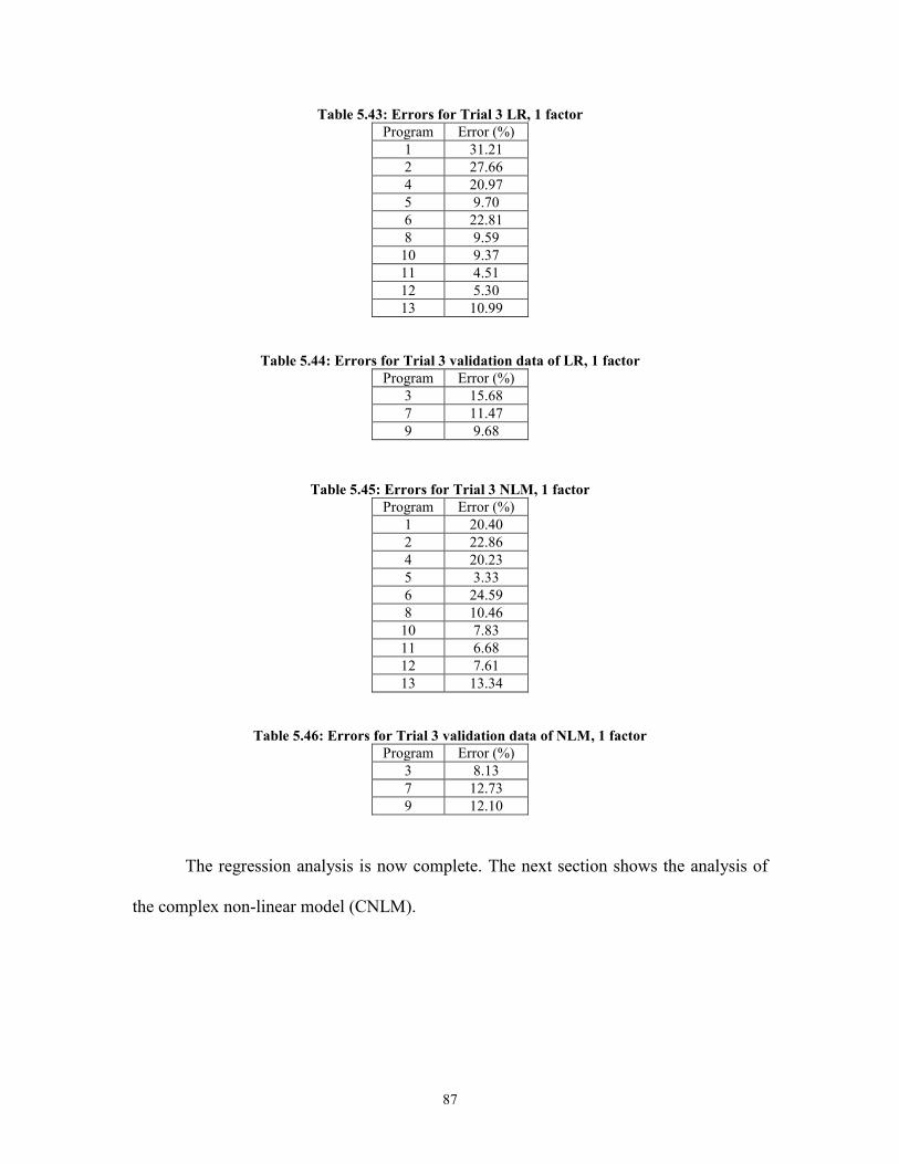
87
Table 5.43: Errors for Trial 3 LR, 1 factor
Program Error (%)
1 31.21
2 27.66
4 20.97
5 9.70
6 22.81
8 9.59
10 9.37
11 4.51
12 5.30
13 10.99
Table 5.44: Errors for Trial 3 validation data of LR, 1 factor
Program Error (%)
3 15.68
7 11.47
9 9.68
Table 5.45: Errors for Trial 3 NLM, 1 factor
Program Error (%)
1 20.40
2 22.86
4 20.23
5 3.33
6 24.59
8 10.46
10 7.83
11 6.68
12 7.61
13 13.34
Table 5.46: Errors for Trial 3 validation data of NLM, 1 factor
Program Error (%)
3 8.13
7 12.73
9 12.10
The regression analysis is now complete. The next section shows the analysis of
the complex non-linear model (CNLM).
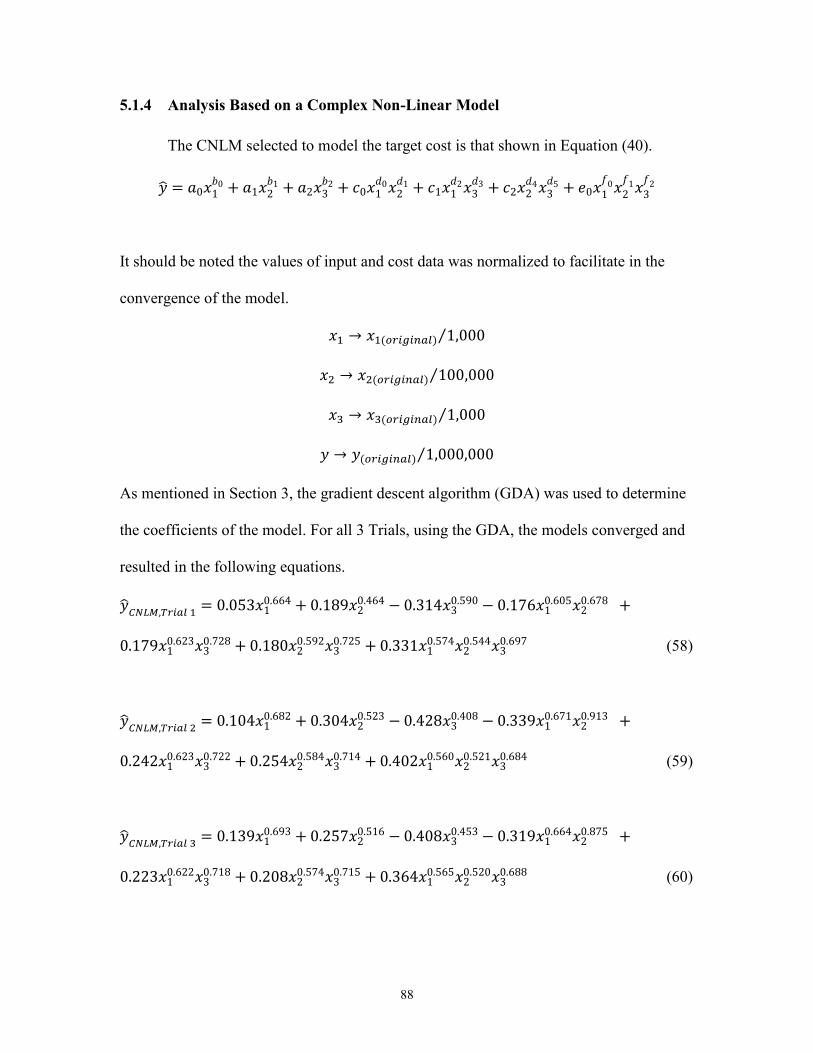
88
5.1.4 Analysis Based on a Complex Non-Linear Model
The CNLM selected to model the target cost is that shown in Equation (40).
It should be noted the values of input and cost data was normalized to facilitate in the
convergence of the model.
⁄
⁄
⁄
⁄
As mentioned in Section 3, the gradient descent algorithm (GDA) was used to determine
the coefficients of the model. For all 3 Trials, using the GDA, the models converged and
resulted in the following equations.
(58)
(59)
(60)

89
The corresponding errors for all the Trials are shown in Tables 5.47 -5.49.
Table 5.47: Errors for Trial 1 CNLM
Program Error (%)
1 7.01
2 4.75
3 12.33
4 14.79
5 3.09
8 10.32
9 0.07
10 6.51
11 4.35
12 11.56
6 23.08
7 9.61
13 13.95
Table 5.48: Errors for Trial 2 CNLM
Program Error (%)
1 1.40
3 1.79
4 0.42
5 0.27
6 0.41
7 1.20
9 2.79
10 1.49
11 0.20
13 1.67
2 0.01
8 1.54
12 0.91
Table 5.49: Errors for Trial 3 CNLM
Program Error (%)
1 11.28
2 9.05
4 19.81
5 12.61
6 10.88
8 1.85
10 5.45
11 4.74
12 2.19
13 5.48
3 14.33
7 2.45
9 5.17

90
The analysis of the parametric CERs is complete. The next section of this thesis
discusses the results obtained to predict the target cost using neural network models.
5.2 Neural Network Model
Several researchers such as Tu (1996), Cavalieri et al. (2004), and Caputo (2008)
have commended neural networks (NN) models for their ability to characterize complex
relationships. Neural network models will be used to estimate the target cost of the MLG
based upon the selected cost drivers. This section will present the results and analysis of
two types of NN models that are trained using 1-back propagation and 2- the genetic
algorithm (GA).
5.2.1 Neural Network Model Trained using Back Propagation
In order use NN, the input and output data must range between 0 and 1. Table
5.50 presents a normalized version of Table 5.1, i.e., the given data.
Table 5.50: Data for NNs
Program x1NN x2NN x3NN yNN
1 0.3184 0.0724 0.6718 0.1280
2 0.4164 0.1820 0.6751 0.2280
3 0.5983 0.4178 0.7867 0.7480
4 0.0722 0.1255 0.0909 0.2754
5 0.1916 0.2325 0.0909 0.6696
6 0.3058 0.2917 0.0699 0.5372
7 0.6731 0.5082 0.1894 0.5226
8 0.6731 0.5932 0.1894 0.6320
9 0.7852 0.6532 0.1911 0.5168
10 0.6640 0.7851 0.3638 0.5350
11 0.3184 0.1086 0.6718 0.1846
12 0.3134 0.2697 0.0798 0.5264
13 0.6640 0.7248 0.3638 0.5349
In order to predict the costs, the final weights are set, via training of the NN
model. The training takes place by using the training data. The first set of training data is
the same as Trial 1 for LR, which omits programs 6, 7, and 13. Similarly, Trials 2 and 3
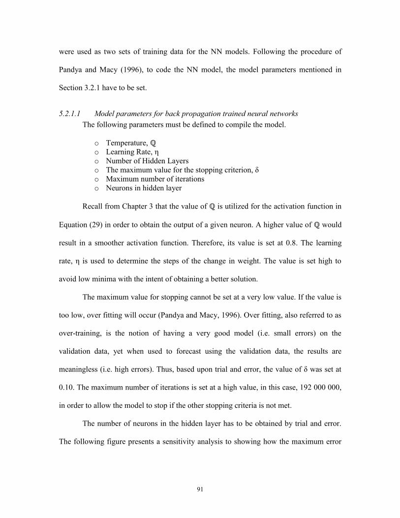
91
were used as two sets of training data for the NN models. Following the procedure of
Pandya and Macy (1996), to code the NN model, the model parameters mentioned in
Section 3.2.1 have to be set.
5.2.1.1 Model parameters for back propagation trained neural networks
The following parameters must be defined to compile the model.
o Temperature,
o Learning Rate, η
o Number of Hidden Layers
o The maximum value for the stopping criterion, δ
o Maximum number of iterations
o Neurons in hidden layer
Recall from Chapter 3 that the value of is utilized for the activation function in
Equation (29) in order to obtain the output of a given neuron. A higher value of would
result in a smoother activation function. Therefore, its value is set at 0.8. The learning
rate, η is used to determine the steps of the change in weight. The value is set high to
avoid low minima with the intent of obtaining a better solution.
The maximum value for stopping cannot be set at a very low value. If the value is
too low, over fitting will occur (Pandya and Macy, 1996). Over fitting, also referred to as
over-training, is the notion of having a very good model (i.e. small errors) on the
validation data, yet when used to forecast using the validation data, the results are
meaningless (i.e. high errors). Thus, based upon trial and error, the value of δ was set at
0.10. The maximum number of iterations is set at a high value, in this case, 192 000 000,
in order to allow the model to stop if the other stopping criteria is not met.
The number of neurons in the hidden layer has to be obtained by trial and error.
The following figure presents a sensitivity analysis to showing how the maximum error

92
on the validation data changes depending of the number of neurons selected in the hidden
layer.
Figure 5.15: Sensitivity Analysis on Neurons in Hidden Layer, Trial 1
All the errors for the sensitivity analysis of Trial 1 are found Table 5.51.
Table 5.51: Sensitivity Analysis of errors for hidden layer, Trial 1
The sensitivity analysis is replicated for Trials 2 and 3. The results of the analysis
are in the following figures and tables.
2.00
2.50
3.00
3.50
4.00
4.50
5.00
5.50
6.00
6.50
7.00
2 3 4 5 6 7 8 9 10 15 20 30
Erro
r (%
)
Neurons in the Hidden Layer
Number of Neurons in the Hidden Layer (N)
2 3 4 5 6 7 8 9 10 15 20 30
Training Max Error 7.15 7.24 7.30 0.00 2.15 3.58 0.93 4.26 5.73 3.78 4.57 6.15
Average Error 1.53 2.18 2.01 0.00 0.47 0.78 0.20 0.94 1.23 0.83 0.99 2.04
Validation Max Error 6.52 4.07 3.40 4.37 2.49 2.49 2.40 2.97 2.74 2.89 3.04 3.69
Average Error 2.90 3.83 3.31 3.64 2.10 2.08 2.07 2.86 2.70 2.59 2.71 2.00
Overall Average Error 1.84 2.56 2.31 0.84 0.85 1.08 0.63 1.39 1.57 1.24 1.39 2.03

93
Figure 5.16: Sensitivity Analysis on Neurons in Hidden Layer, Trial 2
Table 5.52: Sensitivity Analysis of errors for hidden layer, Trial 2
Figure 5.17: Sensitivity Analysis on Neurons in Hidden Layer, Trial 3
8.00
9.00
10.00
11.00
12.00
13.00
14.00
15.00
16.00
17.00
18.00
2 3 4 5 6 7 8 9 10 15 20 30
Erro
r (%
)
Neurons in the Hidden Layer
2 3 4 5 6 7 8 9 10 15 20 30
Max Error 17.19 7.07 5.86 4.91 0.00 18.46 18.79 19.40 2.85 19.54 0.00 2.51
Average Error 9.25 1.53 1.48 1.21 0.00 9.76 9.54 10.15 1.11 9.70 0.00 0.94
Max Error 16.90 16.01 13.77 10.77 14.79 17.16 17.03 17.31 10.08 16.84 16.48 10.54
Average Error 8.39 7.33 8.89 8.11 8.59 8.46 8.46 8.49 8.08 8.06 9.50 7.15
9.05 2.87 3.19 2.80 1.98 9.46 9.29 9.76 2.72 9.32 2.19 2.37
Training
Validation
Overall Average Error
Number of Neurons in the Hidden Layer (N)
8.50
9.00
9.50
10.00
10.50
11.00
11.50
12.00
12.50
2 3 4 5 6 7 8 9 10 15 20 30
Erro
r (%
)
Neurons in the Hidden Layer
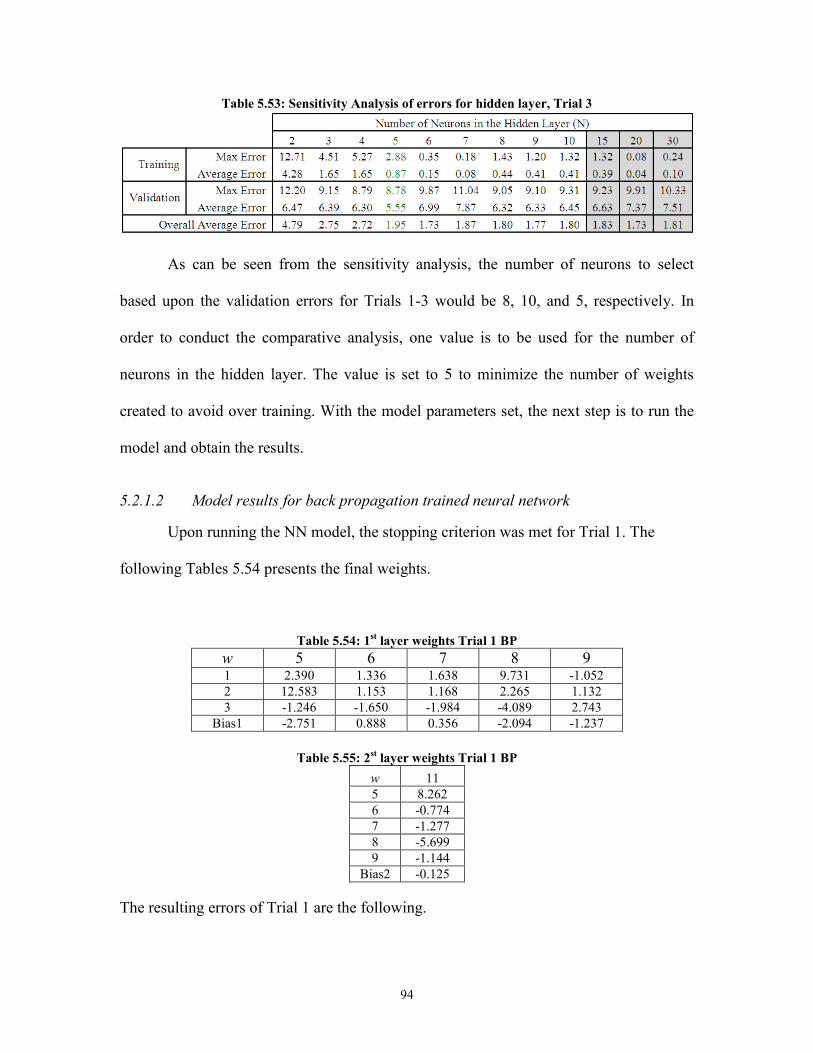
94
Table 5.53: Sensitivity Analysis of errors for hidden layer, Trial 3
As can be seen from the sensitivity analysis, the number of neurons to select
based upon the validation errors for Trials 1-3 would be 8, 10, and 5, respectively. In
order to conduct the comparative analysis, one value is to be used for the number of
neurons in the hidden layer. The value is set to 5 to minimize the number of weights
created to avoid over training. With the model parameters set, the next step is to run the
model and obtain the results.
5.2.1.2 Model results for back propagation trained neural network
Upon running the NN model, the stopping criterion was met for Trial 1. The
following Tables 5.54 presents the final weights.
Table 5.54: 1st layer weights Trial 1 BP
w 5 6 7 8 9 1 2.390 1.336 1.638 9.731 -1.052
2 12.583 1.153 1.168 2.265 1.132
3 -1.246 -1.650 -1.984 -4.089 2.743
Bias1 -2.751 0.888 0.356 -2.094 -1.237
Table 5.55: 2
st layer weights Trial 1 BP
w 11
5 8.262
6 -0.774
7 -1.277
8 -5.699
9 -1.144
Bias2 -0.125
The resulting errors of Trial 1 are the following.
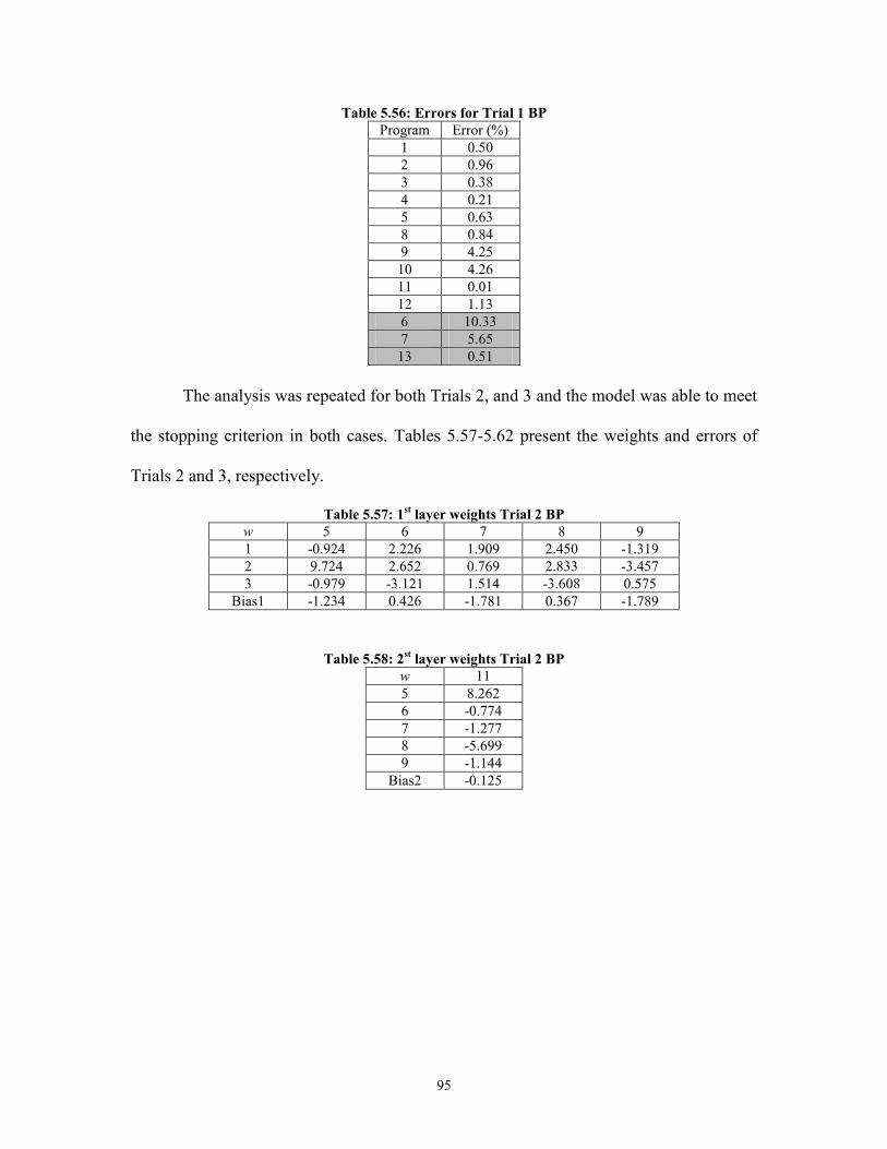
95
Table 5.56: Errors for Trial 1 BP
Program Error (%)
1 0.50
2 0.96
3 0.38
4 0.21
5 0.63
8 0.84
9 4.25
10 4.26
11 0.01
12 1.13
6 10.33
7 5.65
13 0.51
The analysis was repeated for both Trials 2, and 3 and the model was able to meet
the stopping criterion in both cases. Tables 5.57-5.62 present the weights and errors of
Trials 2 and 3, respectively.
Table 5.57: 1st layer weights Trial 2 BP
w 5 6 7 8 9
1 -0.924 2.226 1.909 2.450 -1.319
2 9.724 2.652 0.769 2.833 -3.457
3 -0.979 -3.121 1.514 -3.608 0.575
Bias1 -1.234 0.426 -1.781 0.367 -1.789
Table 5.58: 2st layer weights Trial 2 BP
w 11
5 8.262
6 -0.774
7 -1.277
8 -5.699
9 -1.144
Bias2 -0.125

96
Table 5.59 Errors for Trial 2 BP
Program Error (%)
1 0.11
3 0.05
4 0.00
5 0.19
6 0.18
7 0.31
9 2.04
10 4.30
11 1.84
13 0.60
2 4.93
8 1.72
12 0.81
Table 5.60: 1st layer weights Trial 3 BP
w 5 6 7 8 9
1 7.232 -2.540 3.576 2.616 9.188
2 15.659 0.961 4.812 1.660 3.591
3 -5.855 -3.069 0.462 -3.435 -5.418
Bias1 -2.616 1.708 -2.631 1.135 -1.366
Table 5.61: 2st layer weights Trial 3 BP
w 11
5 6.937
6 3.363
7 3.511
8 -3.81
9 -6.701
Bias2 -1.253
Table 5.62 Errors for Trial 3 BP
Program Error (%)
1 0.01
2 0.24
4 0.18
5 0.32
6 0.34
8 0.38
10 4.91
11 4.56
12 0.74
13 0.40
3 10.77
7 7.61
9 5.96

97
As all 3 trials were able to meet the stopping criterion, the analysis is complete.
The next analysis to be conducted is using a NN trained by the genetic algorithm.
5.2.2 Neural Network Model Trained using the Genetic Algorithm
The data set presented in Table 5.50 will be used for this analysis. For analysis
purposes the same 3 Trials will be utilized. Similar to back propagation, the model
parameters described in Section 3.2.2 are set, with the exception of the learning rate, η.
5.2.2.1 Model parameters for neural networks trained using the GA
In addition to the parameters already set in Section 5.2.1.2, the following
parameters must be defined to compile the model using the genetic algorithm as defined
in Section 3.2.2.
o Maximum step size θmax
o Selection Operator
Population size, n
k-way tournament factor, k
o Cross over operator
Probability of SwCO-1, α1
Probability of SwCO-2, α2
Probability of SPCO-1, α3
Probability of SPCO-1, α4
o Mutation operator
Probability of chromosome being mutated , α5
Probability of gene being mutated, α6
The maximum step is discussed in Section 3.2.2. It is similar to the learning rated
in the NN using back propagation. The value of θmax is set at 0.50. The population size, n
should be a large number in order for the model to develop enough pairs (parents). Since
the GA is compared to the notion of “survival of the fittest,” the selected value of k is

98
small, in this case 0.001, as it is the multiplicative factor to the population to select the
amount of the chromosomes to be randomly selected from the population. The “fittest” or
the one that estimates the cost most accurately will be kept and the remaining will be
discarded, at each iteration.
The crossover operator is the key operator to generate the new population (Dawid,
1996). The probability of all four of the above mentioned operators discussed in detail in
Section 3.2 will have a value of 0.85. Dawid (1996) further explains the mutation
operators should have low probabilities. The probability of a chromosome being mutated
is set at 0.30. Given that the chromosome is mutated, the probability of any given gene
being mutated is 0.15. The model is initialized and the following section presents the
results.
5.2.2.2 Model results for neural network model using the GA
Upon running the model, it converged for all of the Trials. Figures 5.18–5.20
displays the masked cost versus the prediction for Trials 1–3, respectively.
Figure 5.18: Masked Cost versus Prediction for Trial 1 GA
55,000
65,000
75,000
85,000
95,000
105,000
115,000
125,000
135,000
1 2 3 4 5 8 9 10 11 12 6 7 13
Co
st
Data ANN
Training Set Validation Set

99
Figure 5.19: Cost versus Prediction for Trial 2 GA
Figure 5.20: Cost versus Prediction for Trial 3 GA
Tables 5.63 – 5.65 present the errors for all of the trials.
55,000
65,000
75,000
85,000
95,000
105,000
115,000
125,000
135,000
1 3 4 5 6 7 9 10 11 13 2 8 12
Co
st
Data ANN
Training Set Validation Set
55,000
65,000
75,000
85,000
95,000
105,000
115,000
125,000
135,000
1 2 4 5 6 8 10 11 12 13 3 7 9
Co
st
Data ANN
Training Set Validation Set

100
Table 5.63 Errors for Trial 1 GA
Program Error (%)
1 6.88
2 4.49
3 10.25
4 2.02
5 10.89
8 2.78
9 0.56
10 2.02
11 0.56
12 0.52
6 9.94
7 4.98
13 0.08
Table 5.64 Errors for Trial 2 GA
Program Error (%)
1 1.40
3 1.79
4 0.42
5 0.27
6 0.41
7 1.20
9 2.79
10 1.49
11 0.20
13 1.67
2 0.01
8 1.54
12 0.91
Table 5.65 Errors for Trial 3 GA
Program Error (%)
1 2.22
2 7.28
4 6.12
5 4.76
6 10.74
8 6.77
10 5.94
11 2.12
12 2.54
13 0.93
3 2.21
7 6.10
9 6.72
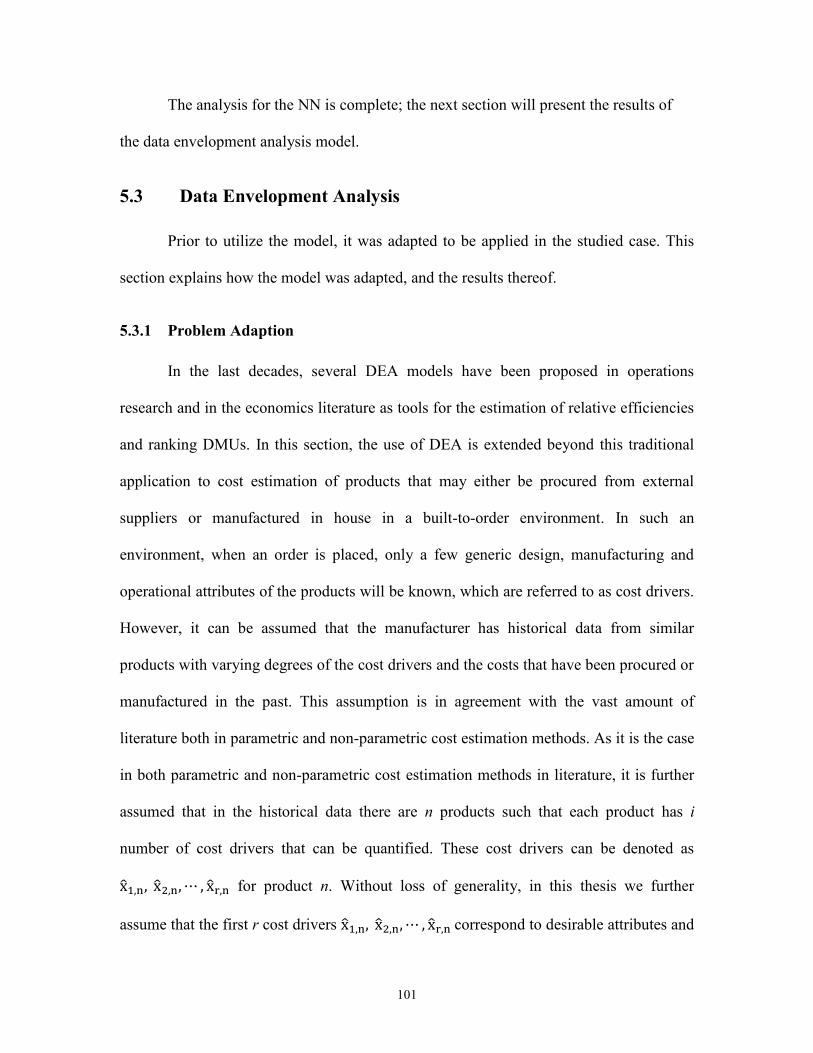
101
The analysis for the NN is complete; the next section will present the results of
the data envelopment analysis model.
5.3 Data Envelopment Analysis
Prior to utilize the model, it was adapted to be applied in the studied case. This
section explains how the model was adapted, and the results thereof.
5.3.1 Problem Adaption
In the last decades, several DEA models have been proposed in operations
research and in the economics literature as tools for the estimation of relative efficiencies
and ranking DMUs. In this section, the use of DEA is extended beyond this traditional
application to cost estimation of products that may either be procured from external
suppliers or manufactured in house in a built-to-order environment. In such an
environment, when an order is placed, only a few generic design, manufacturing and
operational attributes of the products will be known, which are referred to as cost drivers.
However, it can be assumed that the manufacturer has historical data from similar
products with varying degrees of the cost drivers and the costs that have been procured or
manufactured in the past. This assumption is in agreement with the vast amount of
literature both in parametric and non-parametric cost estimation methods. As it is the case
in both parametric and non-parametric cost estimation methods in literature, it is further
assumed that in the historical data there are n products such that each product has i
number of cost drivers that can be quantified. These cost drivers can be denoted as
for product n. Without loss of generality, in this thesis we further
assume that the first r cost drivers correspond to desirable attributes and

102
the remaining i – r cost drivers correspond to undesirable
attributes. A desirable attribute means, that given all other attributes kept unchanged, the
higher the value of this attribute, the better it is (e.g. load carrying capacity) and the
opposite applies for undesirable attributes (e.g. weight of a sub-assembly). With the
above introduction, an adapted version of the problem is presented. The analogy between
a DMU and a product is used for the purpose of using DEA as a cost estimation tool.
5.3.1.1 Input Adaptation
For DMUk, given all else is equal, the lesser an input quantity xi,k is the more
efficient this DMU. For PRODUCTk, given all else is equal, the higher a desirable
attribute (for i ≤ r) or the lesser an undesirable attribute (for i > r), the better is
the product. If we make an analogy between DMUk and PRODUCTk, then the inputs to
the product should be ⁄ for i ≤ r and xi,k = for i > r so that the lesser an
input can be interpreted as the better product as is the case for DMUk. This input
adaptation is summarized in Equation (61).
{
} (61)
5.3.1.2 Output Adaption
For DMUk, given all other inputs and outputs the same, the higher an output yo,k
is, the more efficient the DMU. For PRODUCTk, given all other inputs the same, the
lower the cost is the better the product. If we make an analogy between DMUk and
PRODUCTk, then the output from PRODUCTk should be y1,k = 1/cost. Thus for this
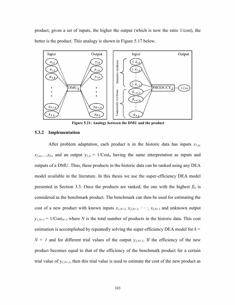
103
product, given a set of inputs, the higher the output (which is now the ratio 1/cost), the
better is the product. This analogy is shown in Figure 5.17 below.
Figure 5.21: Analogy between the DMU and the product
5.3.2 Implementation
After problem adaptation, each product n in the historic data has inputs x1,n,
x2,n,…,xI,n and an output y1,n = 1/Costn having the same interpretation as inputs and
outputs of a DMU. Thus, these products in the historic data can be ranked using any DEA
model available in the literature. In this thesis we use the super-efficiency DEA model
presented in Section 3.3. Once the products are ranked, the one with the highest Ek is
considered as the benchmark product. The benchmark can then be used for estimating the
cost of a new product with known inputs x1,N+1, x2,N+1, · · ·, xI,N+1 and unknown output
y1,N+1 = 1/CostN+1 where N is the total number of products in the historic data. This cost
estimation is accomplished by repeatedly solving the super-efficiency DEA model for k =
N + 1 and for different trial values of the output y1,N+1. If the efficiency of the new
product becomes equal to that of the efficiency of the benchmark product for a certain
trial value of y1,N+1, then this trial value is used to estimate the cost of the new product as
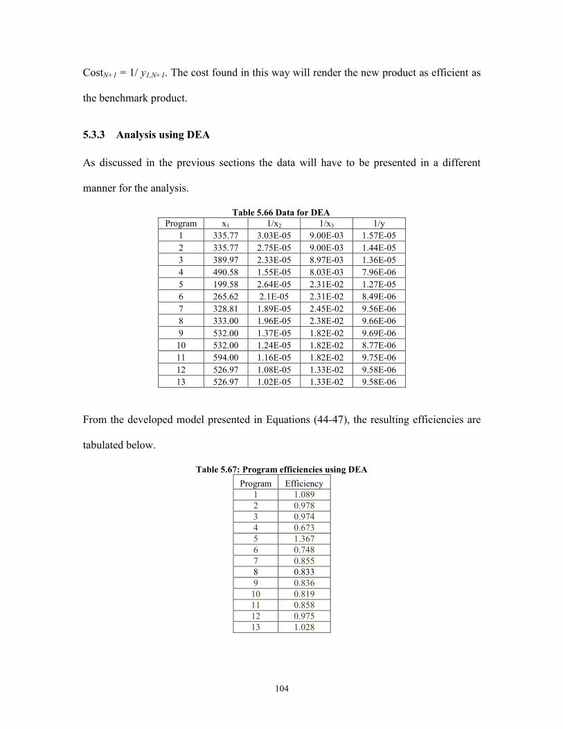
104
CostN+1 = 1/ y1,N+1. The cost found in this way will render the new product as efficient as
the benchmark product.
5.3.3 Analysis using DEA
As discussed in the previous sections the data will have to be presented in a different
manner for the analysis.
Table 5.66 Data for DEA
Program x1 1/x2 1/x3 1/y
1 335.77 3.03E-05 9.00E-03 1.57E-05
2 335.77 2.75E-05 9.00E-03 1.44E-05
3 389.97 2.33E-05 8.97E-03 1.36E-05
4 490.58 1.55E-05 8.03E-03 7.96E-06
5 199.58 2.64E-05 2.31E-02 1.27E-05
6 265.62 2.1E-05 2.31E-02 8.49E-06
7 328.81 1.89E-05 2.45E-02 9.56E-06
8 333.00 1.96E-05 2.38E-02 9.66E-06
9 532.00 1.37E-05 1.82E-02 9.69E-06
10 532.00 1.24E-05 1.82E-02 8.77E-06
11 594.00 1.16E-05 1.82E-02 9.75E-06
12 526.97 1.08E-05 1.33E-02 9.58E-06
13 526.97 1.02E-05 1.33E-02 9.58E-06
From the developed model presented in Equations (44-47), the resulting efficiencies are
tabulated below.
Table 5.67: Program efficiencies using DEA
Program Efficiency
1 1.089
2 0.978
3 0.974
4 0.673
5 1.367
6 0.748
7 0.855
8 0.833
9 0.836
10 0.819
11 0.858
12 0.975
13 1.028
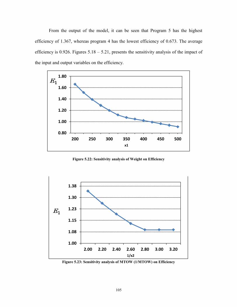
105
From the output of the model, it can be seen that Program 5 has the highest
efficiency of 1.367, whereas program 4 has the lowest efficiency of 0.673. The average
efficiency is 0.926. Figures 5.18 – 5.21, presents the sensitivity analysis of the impact of
the input and output variables on the efficiency.
Figure 5.22: Sensitivity analysis of Weight on Efficiency
Figure 5.23: Sensitivity analysis of MTOW (1/MTOW) on Efficiency
0.80
1.00
1.20
1.40
1.60
1.80
200 250 300 350 400 450 500
x1
1.00
1.08
1.15
1.23
1.30
1.38
2.00 2.20 2.40 2.60 2.80 3.00 3.20
1/x2
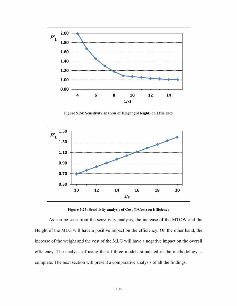
106
Figure 5.24: Sensitivity analysis of Height (1/Height) on Efficiency
Figure 5.25: Sensitivity analysis of Cost (1/Cost) on Efficiency
As can be seen from the sensitivity analysis, the increase of the MTOW and the
Height of the MLG will have a positive impact on the efficiency. On the other hand, the
increase of the weight and the cost of the MLG will have a negative impact on the overall
efficiency. The analysis of using the all three models stipulated in the methodology is
complete. The next section will present a comparative analysis of all the findings.
0.80
1.00
1.20
1.40
1.60
1.80
2.00
4 6 8 10 12 14
1/x3
0.50
0.70
0.90
1.10
1.30
1.50
10 12 14 16 18 20
1/y
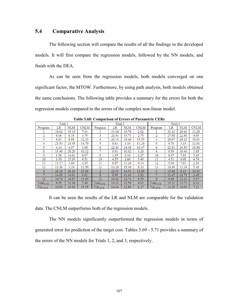
107
5.4 Comparative Analysis
The following section will compare the results of all the findings in the developed
models. It will first compare the regression models, followed by the NN models, and
finish with the DEA.
As can be seen from the regression models, both models converged on one
significant factor, the MTOW. Furthermore, by using path analysis, both models obtained
the same conclusions. The following table provides a summary for the errors for both the
regression models compared to the errors of the complex non-linear model.
Table 5.68: Comparison of Errors of Parametric CERs
It can be seen the results of the LR and NLM are comparable for the validation
data. The CNLM outperforms both of the regression models.
The NN models significantly outperformed the regression models in terms of
generated error for prediction of the target cost. Tables 5.69 - 5.71 provides a summary of
the errors of the NN models for Trials 1, 2, and 3, respectively.
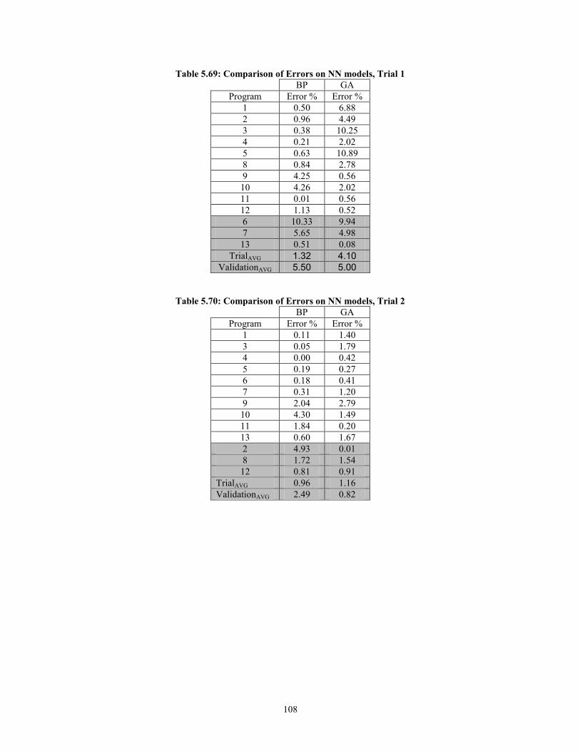
108
Table 5.69: Comparison of Errors on NN models, Trial 1
BP GA
Program Error % Error %
1 0.50 6.88
2 0.96 4.49
3 0.38 10.25
4 0.21 2.02
5 0.63 10.89
8 0.84 2.78
9 4.25 0.56
10 4.26 2.02
11 0.01 0.56
12 1.13 0.52
6 10.33 9.94
7 5.65 4.98
13 0.51 0.08
TrialAVG 1.32 4.10
ValidationAVG 5.50 5.00
Table 5.70: Comparison of Errors on NN models, Trial 2
BP GA
Program Error % Error %
1 0.11 1.40
3 0.05 1.79
4 0.00 0.42
5 0.19 0.27
6 0.18 0.41
7 0.31 1.20
9 2.04 2.79
10 4.30 1.49
11 1.84 0.20
13 0.60 1.67
2 4.93 0.01
8 1.72 1.54
12 0.81 0.91
TrialAVG 0.96 1.16
ValidationAVG 2.49 0.82
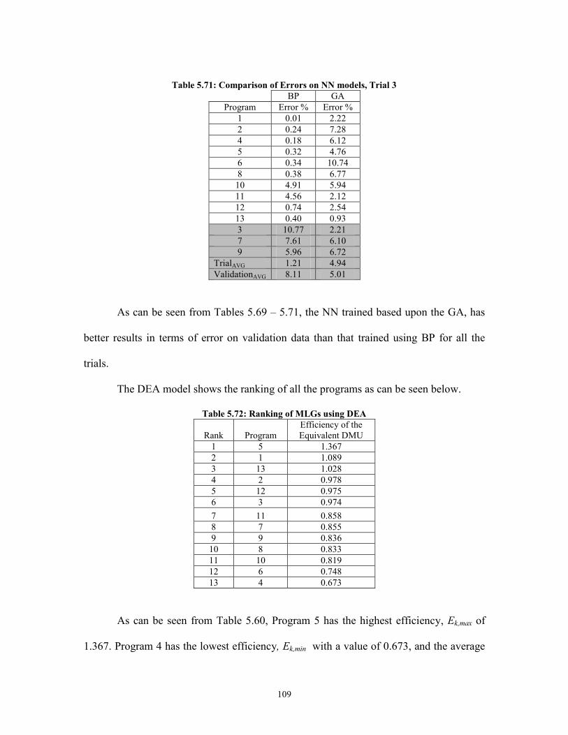
109
Table 5.71: Comparison of Errors on NN models, Trial 3
BP GA
Program Error % Error %
1 0.01 2.22
2 0.24 7.28
4 0.18 6.12
5 0.32 4.76
6 0.34 10.74
8 0.38 6.77
10 4.91 5.94
11 4.56 2.12
12 0.74 2.54
13 0.40 0.93
3 10.77 2.21
7 7.61 6.10
9 5.96 6.72
TrialAVG 1.21 4.94
ValidationAVG 8.11 5.01
As can be seen from Tables 5.69 – 5.71, the NN trained based upon the GA, has
better results in terms of error on validation data than that trained using BP for all the
trials.
The DEA model shows the ranking of all the programs as can be seen below.
Table 5.72: Ranking of MLGs using DEA
Rank Program
Efficiency of the
Equivalent DMU
1 5 1.367
2 1 1.089
3 13 1.028
4 2 0.978
5 12 0.975
6 3 0.974
7 11 0.858
8 7 0.855
9 9 0.836
10 8 0.833
11 10 0.819
12 6 0.748
13 4 0.673
As can be seen from Table 5.60, Program 5 has the highest efficiency, Ek,max of
1.367. Program 4 has the lowest efficiency, Ek,min with a value of 0.673, and the average

110
efficiency, Ek,avg of all the programs is 0.926. With the efficiencies stated above, for all
programs the actual cost, y is compared to the target cost, based upon the different
efficiencies, and is shown in Table 73.
Table 5.73: Cost based upon varying Efficiencies
Program y
1 63,816 50,801 103,235 75,046
2 69,465 49,687 100,971 73,400
3 73,794 52,549 106,787 77,628
4 125,657 61,835 125,657 91,344
5 78,516 78,516 159,555 115,987
6 117,834 64,491 131,054 95,268
7 104,635 65,426 132,954 96,649
8 103,552 63,065 128,157 93,162
9 103,173 63,110 128,250 93,229
10 114,082 68,327 138,851 100,936
11 102,595 64,410 130,890 95,149
12 104,400 74,416 151,223 109,930
13 104,408 78,498 159,519 115,960
This concludes the comparative analysis of the models.
5.5 Chapter Summary
This chapter presented the results of the three methodologies used in this thesis. It
presents the results on regression analysis, which was followed by the analysis of neural
networks, followed by the findings on data envelopment analysis. Finally, it presents a
comparative analysis of the aforementioned models. The next chapter will present a
general discussion of the findings in this thesis.
111
6. Discussion and Implications
This chapter discusses how the results of the models can be applied in a more
generalizable way, and the implications thereof. This chapter will begin by presenting the
summary of findings, followed by practical applications, and concluded by the
managerial implications.
6.1 Summary of Findings
Many qualitative and quantitative studies have been conducted pertaining to the
cost of commodities. Research in this area has been even more emphasized over the last
two decades with the increased advent of low cost countries in the global economy. In
order to reduce or contain total acquisition costs, much emphasis has been placed on
target costing.
This thesis presents three different methodologies for determining target costs and
compares the performance of each. Even though this research is applied to a specific
commodity, the findings and approach utilized can be applied in a general fashion.
The first methodology under study was utilizing parametric based analysis to
develop two regression models, one based on a multiple linear regression equation, and
the second based on a non-linear equation. From Section 5.1 it was found that the results
of both models were comparable. However, these findings are not in line with Salam et
al. (2008, 2009), in which the non-linear models clearly outperformed the linear ones.
This analysis highlights the sensitivity of parametric models based on linear regression.
These findings suggest that there is no general rule for which a model is better, in or other
words, “One size does not fit all.”

112
The findings also demonstrate the mediocre results in predicting costs,
highlighting the need for more accurate models which can take into account the intricate
relationships of the given variables, in this case, the cost drivers. Finally, it may question
regression models in general as being the sole reference point in establishing the target
cost. The manner of overcoming the shortcomings of the regression models was to
develop models based upon neural networks.
The models based on neural networks had more meaningful results. Two types of
training techniques were applied in developing the models. The first model was trained
using the back propagation method, and the second model was trained using the genetic
algorithm. Compared to the regression models, the NN models trained using BP reduced
the overall prediction error roughly by a factor of four. These findings were in line with
the results of Chou et al. (2010). However, it was not in line with their perception of
questioning the validity of NN models with small sample sizes, as to overcome this
hurdle several trials were conducted, and they all yielded meaningful results.
When NN model using BP was compared to that using the GA, it was found that
the latter yielded superior results. As there was no real benchmark found in cost
estimation in the comparison of the two models, the research was compared to the
findings applied in other domains. The other domains used for comparison were those of
data classification, manufacturing, and healthcare. The research findings in these domains
all concurred with those found in this thesis (Örkcü and Bal, 2011; Provorovs and
Borisov, 2011; Fu and Liu, 2011; Zhang et al., 2012; Ahmad et al., 2010). This suggests
in general that NN models trained using the GA have better and more meaningful results
than those trained with the BP training algorithm.
113
The final model that was developed based on data envelopment analysis was
created to calculate the efficiency of the programs. Based upon the findings of the
efficiencies, the programs were ranked. Moreover the efficiencies can be used to predict
the target cost for development programs. Based on the analysis, the ranking, in terms of
efficiency using the cost and their associated drivers was established, and comparable to
the research of Sueyoshia and Goto (2011) and Kao (2012). The findings of the DEA
models as well the findings of the regression and neural network models can have several
practical applications, as well as managerial implications, which are discussed in the
following section.
6.2 Practical Applications and Managerial Implications
There can be several applications of the findings of this research in an industrial
setting. After developing the target cost model and successfully applying it for the MLG,
BA wanted to apply them to several other commodities. The other commodities include
the engines, the auxiliary power unit (APU), and the wings. The models were accurate in
the range of 10%, which is considered reasonable given the estimates are to be used for
development programs. Given the successful application of these models on several real
components, it can be suggested that they are applicable to products in any industry. Any
product generally will have key characteristics that influence its cost. Upon identifying
these cost drivers, the methodology used in this thesis can be followed.
Furthermore, the analysis of this case can be applied in trade-off studies, budget
allocation, supplier negotiations, and can even further be extended into supplier selection,
given support for management.

114
6.2.1 Trade-off Studies
When designing a product, several trade-off studies have to be conducted usually
to optimize the performance and dimensions of the particular product. According to the
FAA, (2006), a trade or trade-off study is the process of selecting an optimal solution
given several viable solutions. A trade-off study is usually initiated at the request of the
market, or the customer.
An example where the target cost was applied in the case company to a trade-off
study was to respond to needs of the market to increase the flying distance (range) of the
aircraft. A trade study was conducted and two of the viable solutions presented were to
either increase the aerodynamic properties of the wing, or to increase the thrust of the
engines. The cost drivers of both the wings and the engines were established. Based on
these, the target costs of the modified design of the wing and the higher performing
engines were calculated. With the target cost models, engineers were able propose a
solution that meets the requirements of the market, while minimizing the associated costs.
These findings can also be applied in a general fashion when trade-off studies
must be conducted; having accurate cost models will help to propose an optimal technical
solution while considering the associated costs thereof.
6.2.2 Budget Allocation
It is of utmost important to understand the total acquisition cost when purchasing
a product or service. The target cost is a key value of the total acquisition cost. It would
allow the proper planning and allocation of the budget, if feasible, for the product or
service to be procured. Using the DEA model would support the notion of “Plan for the
worst, and hope for the best.” By varying the efficiency, a price range could be
115
established to estimate the most and least they should expect to pay for a particular
product. This price range would allow the personnel responsible for the budget to allocate
the higher price point in their budget. However, the lower price can be set as targets for
suppliers.
6.2.3 Negotiation with Suppliers
“Any negotiation is 80% preparation and only 20% execution” is a phrase
commonly stated by executives at Bombardier Aerospace. In any given industry,
historical negotiations with suppliers have been based on the market price for a given
commodity, with little focus on the actual cost of the product or service. Having an
accurate cost model completely changes the dynamics of the negotiation at hand. Using
the developed target cost models, the company was able to have fact-based negotiations
with their suppliers.
Establishing targets for suppliers had significant benefits in the outcome of
commercial negotiations. As the target cost will be a key element in the total life cycle
cost model, the company was able to measure the suppliers against the targets and rank
them for comparison purposes. Without divulging any proprietary information, using this
methodology for several commodities resulted in significant savings on the total life
cycle cost from the suppliers initial bid to the signed agreement. For some commodities,
the savings could be in range of 50%, which is rather significant, considering that these
commodities cost thousands, or even millions of dollars per unit.
116
6.2.4 Supply Base Optimization
This research can also be extended and applied to reducing the number of
considered suppliers. In the aerospace industry depending on the commodity, the range of
potential suppliers vastly varies anywhere from 1 to thousands. Having too many
suppliers may be difficult to manage and moreover may be very costly, such as in indirect
services like facilities maintenance, consulting, and recruitment, where dozens of
potentials suppliers may exist. From the findings of the DEA model, along with the
associated target cost models, an organization may be able to determine with suppliers
will be able to meet the target cost. Furthermore, with the intent of reducing the effort in
procuring a product (or service), the organization can shortlist suppliers to only those
they believe will be able to meet the target costs.
6.2.5 Managerial Implications and Support
In order to derive the most benefits out of the outcomes of this research, there has
to be support from management. As this case was applied for a particular commodity, it
was also applied for other commodities, and the findings had several implications
As discussed in the previous section, with the data envelopment analysis model,
suppliers that will not be able to meet the cost targets can be identified. Based on the
findings in this thesis, management may suggest eliminating the dealings or consideration
of those suppliers for future products that are unable to meet the targets. Management
may want to consolidate their list of suppliers to develop a preferred supplier list.
However, internal stakeholders may have their own preferred or favourites, and may be
emotionally or personally involved in the decision process, making it very difficult for

117
management to decide and execute the elimination of those suppliers for future dealings,
as the decision may become very political.
Another challenge as was faced in this case in getting the buy in from
management to rely on the target cost models derived from neural networks. Even though
the NN models outperform the regression models, the regression models will be more
readily accepted for application to other commodities. There are several reasons for the
push back from management. Linear regression models may not be the best predictors but
the cost estimating relationships are clearly defined. It is relatively easy to understand the
relationship that a cost driver has on the cost while using a linear, or even a non-linear
model, when compared to neural networks.
The costs drivers in the regression model are tangible and are easy to get a grasp
of, whereas, neural network models are intangible and the calculations taking place in the
“black box” cannot be seen, thus it intuitively becomes difficult to rely on or comprehend
the resulting target cost models. Due to the above-mentioned reasons, coupled with the
difficulty in replicating the results on the NN models, and because of its random
component, it is a tough sell and will be a paradigm shift for management to solely rely
on target cost models utilizing neural networks. When management accepts the models,
they will also face similar challenges in convincing their internal stakeholders as well as
their suppliers with whom they have an open book approach. This dilemma still exists
today and was highlighted by Smith and Mason (1997).
Finally, as the importance of identifying the cost drivers has been highlighted
several times throughout this thesis, due its direct relation to the credibility and accuracy
of its associated cost model effort and time will have to be allocated by management, for
118
any given study, in properly identifying the cost drivers. Moreover, as was seen in this
case, the process of identifying the cost drivers, along with data collection, will require
the support of many stakeholders from several parts of the organization. Management
will need to align the internal priorities to support this endeavour.
6.3 Chapter summary
This chapter discussed the findings of the target cost models developed in this
thesis. Furthermore, the practical applications in terms of trade-off studies, budget
allocation, negotiation and even extending into supplier selection were discussed.
Moreover, it highlights the implication of using, and implementing, the developed
models. Finally it ends by describing the tactical issues management may face in the
development of the target cost models.

119
7. Conclusions
The aerospace industry is very important for Canada. Currently the market is
facing many challenges; the economic downturns coupled with the advent of emerging
countries entering the market have made it very difficult for companies in Canada to keep
a competitive advantage. Their revenues have dropped over the last few years and they
are trying to survive the crisis. In order to face these challenges they are adopting new
principles to reduce costs and remove the waste in their organizations.
The traditional cost plus approach, in which the selling price of a product is
established only after its development by adding the desired profit margin, may result in
not being competitive in the market, thus not focusing on delivering value to their
customers. The lean accounting approach, based on the principles of lean manufacturing,
to deliver value to their customer, overcomes these weaknesses. By establishing a target
cost of the product on the basis of what the market can bear, they will focus on how to
design the product and its key characteristics to deliver value to the customer. Thus, the
target cost is in line with the principles of lean. The focus of this thesis was lean
accounting in aerospace, and on accurately predicting target costs.
In this thesis, several models to predict target costs for commodities are presented
and applied at a major aerospace company, Bombardier Aerospace, the world‟s third
largest civil aircraft manufacturer specializing in the manufacture and assembly of both
commercial and business aircrafts.
In this thesis, three models are developed to estimate target cost, each of which is
applied to the main landing gear at Bombardier. In order to develop the target cost, the

120
pertinent cost drivers were obtained. This thesis shows the necessary steps and
demonstrates the rigour in obtaining the right cost drivers.
The first methodology used to develop target cost models is linear regression.
Two regression models are developed. The first model is based on a multiple linear
regression model, and the second is based on a non-linear equation. A sub-sampling
method, namely the jackknife technique is used to increase the accuracy of the models.
Moreover, three data points are removed from the analysis, and are used to calculate the
accuracy in predicting the costs.
Thereafter, two techniques are chosen to determine the number of factors to be
kept in the final cost models. The two techniques both recommend keeping one cost
driver, namely the maximum take-off weight, in the regression models. The results show
that both models have comparable yet mediocre results. To complement the regression
models, a complex non-linear model was developed. Its overall performance was superior
to those of the regression models; however it did contain some high errors.
In order to overcome the shortcomings of these models, two artificial neural
networks based on different training algorithms are developed. The first training
mechanism is that of error back propagation, and the second is trained using the genetic
algorithm. Three trials are conducted, and the both neural network models increase the
accuracy of the prediction by at least a factor of 4. When compared to one another, the
genetic algorithm outperforms that of back propagation. This research also questions the
claims of other researchers‟ statements of not being able to derive meaningful results
using limited data, like that presented in the case. Moreover, the sensitivity analysis of
the number of neurons in the hidden layer showed a minimal impact on the final model,

121
which is also contrary to previous research, indicating the high sensitivity of neurons in
the hidden layer.
The final model developed is based on a modified version of the traditional data
envelopment analysis model, to rank the programs in order of their efficiency, and thus,
the target cost. With this model, the suppliers are ranked and target costs can be
predicted.
The models were developed using the cost drivers. In this case, the cost drivers
were height, maximum take-off weight, and weight for the main landing gear; the data of
13 programs is collected for the analysis. The commercial data was masked to protect
proprietary information.
The cost models yielded accurate results, and thus the analysis was repeated for
other commodities. The cost models for the other commodities (wings, engines, and the
auxiliary power units) had reasonable estimates, with errors in the magnitude of 10%.
From the finding of the analysis there are several practical applications, of which some
were already implemented. The practical applications pertain to using the cost models to
conduct trade-off studies, allocation of budget, negotiation tools and even extending the
use of the models to determine the suppliers to be considered for future dealings.
While the analysis highlights the importance of obtaining the pertinent cost
drivers, it also hints to the amount of time and effort required from many stakeholders
across the organization. This may require the support from management to align the
priorities across the domains to get the required support for these initiatives. Finally this
thesis also highlights the challenges faced when proposing to implement the target cost
models based upon artificial neural network models.
122
This research shows that regression models are very sensitive and a non-linear
model may not necessarily outperform a linear model when estimating the cost.
Furthermore, by using two different neural network models, it was shown the models
trained by the genetic algorithm had more meaningful results. Research applied in other
domains has also indicated NN trained with the GA has outperformed those using the BP
training algorithm. The findings of this research coupled previous studies infers that
models trained using the genetic algorithm will always outperform those models trained
using back propagation. Finally an adapted version of the DEA model was developed.
This model ranks suppliers, but it can also be used as a mechanism to predict the target
cost.
Even though the models have promising results, there are limitations to the model.
The model is only as good as its input data. This highlights the sensitivity and credibility
of the model depending upon the right cost drivers. If the wrong cost drivers are selected,
the results will be of no value. Moreover as the cost drivers differ from commodity to
commodity they have to be identified each time and the neural network models may need
to be tuned from one commodity to another. Furthermore, using parametric analysis, the
predetermined relationship, such as linear, non-linear or exponential has to be specified.
Thus other complex relationships exist; the regression models will have limited use.
Finally, the underlying assumptions of the CERs are that the data and cost drivers
selected in the final model will be representative of the cost of the future. It does not take
into any design or technological changes that will potentially change the cost drivers,
which will limit the use of the developed models. Moreover, the focus of the target cost
models is for the recurring costs only. The non-recurring costs, such as the design and

123
testing of the commodity are not taken into account in the cost models. The non-recurring
costs are typically considered as stand-alone items in the business case, and are allocated
at the aircraft level based upon the sales forecast. However, other models, as mentioned
in the literature review, have been and can be further developed, to account for those
costs.
Even though the NN models predicted the costs reasonably, they also have their
limitations. Many parameters have to be set, in order to train the model. If the parameters
are not set appropriately, the results can be skewed, and the NN models be trapped in the
local minima, not being able to find a better solution. This can partially be overcome by a
sensitivity analysis and by trial and error, as was done in this case, to partially overcome
this limitation.
There can be several future applications of this thesis. Higher order parametric
models can be developed to estimate the target cost. As the regression models did not
take into complex relationships. The use of higher order model would allow to model
complex relationships that may exist and are not accounted for in the regression-based
models.
Moreover, there are other types of training algorithms such as simulated
annealing, which can be used in the neural network models to develop the target cost.
The models developed using various training mechanisms can be applied to see if they
are able to predict the cost better than those presented in the case. Finally, as the neural
network models presented in this thesis have a fixed mechanism to sequentially adjust the
weights, an adaptive weight adjustment technique can be used to see the impact on the
accuracy of the developed target cost models.

124
REFERENCES
P. Ahlstrom, C. Karlsson, Change processes towards lean production: the role of the
management accounting system, International Journal of Production and Operations
Management, vol. 16, no. 11, pp. 42-56, 1996
F. Ahmad, N. A. M. Isa, M. K. Osman, Z. Hussain, Performance comparison of gradient
descent and genetic algorithm based artificial neural networks training, 10th
International
Conference on Intelligent Systems Design and Applications (ISDA), 2010.
AIAC, Aerospace Industries Association of Canada, 2002[www.aiac.ca/corporate-
membershp/aiac-mebers. Latest access 04/06/12]
P. Andersen, N. C. Petersen, A procedure for ranking efficient units in data envelopment
analysis, Management Science, vol. 39, no. 2, 1993.
C. Ax, J. Greve, U. Nilsson, The impact of competition and uncertainty on the adoption
of target costing, International Journal of Production Economics, vol. 115 no. 1, pp. 92–
103, 2008.
A. Bahadir, The role of management accounting systems in implementing lean business
strategies, Master‟s Thesis, Erasmus University, Rotterdam, 2011.
H. A. Bashir, V. Thomson, Estimating design effort for GE hydro projects, Computers &
Industrial Engineering, vol. 46, no. 2, pp. 195-204, 2004.
Y. Beauregard, N. Bhuiyan, V. Thomson, Lean engineering in product development,
Canadian Aeronautics and Space Journal, vol. 54, no. 2, pp. 19-30, 2008.
Y. Beauregard, A multi-criteria performance study of lean engineering, PhD thesis,
Concordia University, Montreal, Canada, April, 2010.
S. J. Benjamin, S. Muthaiyah, M. S. Marathamuthu, An improved methodology for
absorption costing: efficiency based absorption costing (EBAC), The Journal of Applied
Business Research, vol. 25, no. 6, pp. 87-104, 2009.
V. S. Berg, Water utility benchmarking: measurement, methodologies, and performance
incentives, International Water Association, 2010.
S. Berg, C. Lin, Consistency in performance rankings: the Peru water sector, Applied
Economics, vol. 40, no. 6, pp. 793-805, 2008.
C. Bi, F. Wei, Civil aircraft maintenance target cost allocation based upon Value
Engineering, Communication Software and Networks (ICCSN), IEEE 3rd International
Conference on Communication Software and Networks, pp. 521 - 524, Xi'an, China,
2011.

125
C. Bishop, Neural networks for pattern recognition, Oxford Press, USA, 1996.
J. T. Black, D. T. Phillips, Introduction to lean engineering, Prentice Hall, 2012.
S. A. Butsher, A. Stephan, M. Laker, Market-driven product development, Marketing
Management, vol. 9, no. 3, pp. 48-54, 2000.
L. P. F. Carmo, F. Cadovani, Advances and challenges for adoption of activity based
costing (ABC) by public sector: a comparative study of Brazil, Colombia, Uruguay and
United States, International Business Research, vol. 5, no. 2, pp. 150-158, 2012.
S. Cavalieri, P. Maccarrone, R. Pinto, Parametric vs. neural network models for the
estimation of production costs: A case study in the automotive industry, International
Journal of Production Economics, vol. 1, pp. 165–177, 2004.
A. C. Caputo, P. M. Pelagagge, Parametric and neural methods for cost estimation of
process vessels, International Journal of Production Economics, vol. 112, pp. 934–954,
2008.
H. K. Chan, S. Yin, F.T.S. Chan, Implementing just-in-time philosophy to reverse
logistics systems: a review, International Journal of Production Research, vol. 48, no. 21,
pp. 6293–6313, 2010.
D. W. M. Chan, A. P. C. Chan, P. T. L. Lam, J. H. L. Chan, Exploring the key risks and
risk mitigation measures for guaranteed maximum price and target cost contracts in
construction, Construction Law Journal, vol. 26, no. 5, pp. 364-378, 2010.
A. Charnes, W. W. Cooper, E. Rhodes, Measuring the efficiency of decision making
units, European Journal of Operations Research, pp. 429-444, vol. 2, 1978.
J. Choe, The taxonomy of knowledge management strategies in manufacturing firms: Use
of target costing and IT Infrastructure, African Journal of Business Management, vol. 15,
no. 5, pp. 6597-6607, 2011.
J. S. Chou, Y. Tai, Generalized regression neural nets in estimating the high-tech
equipment project cost, Computer Engineering and Applications (ICCEA), 2010 Second
International Conference on Computer Engineering and Applications, pp. 281-284, Bali
Island, 2010.
G. Cokins, S. Căpuşneanu, C-M. Barbu, Decisions based on synthesis documents
information of the ABC (activity-based costing) method, International Journal of
Accounting and Financial Reporting, vol. 1, no. 1, pp. 112-132, 2011.
Conference Board of Canada, Canadian Aerospace industry contends with slow rebound
in demand and fierce global competition, News Release, pp. 12-67, 2011.
126
R. Cooper, B. H. Maskell, How to manage through worse-before-better, MIT Sloan
management review, vol. 49, no. 4 , pp. 58-65, 2008.
N. S. Currey, Aircraft landing gear design: principles and practices, 1988.
H. Dawid, Adaptive learning by genetic algorithms: analytical results and applications to
economic models, Springer, New York, 1996.
G. K. DeBusk, use lean accounting to add value to the organization, The Journal of
Corporate Accounting & Finance, vol. 23, no. 3, pp. 35–41, 2012.
J. DeFilippo, Management accounting learns to adapt to Pratt & Whitney‟s
manufacturing cells, The Learning Organization, vol.3, no.2, pp. 4-10, 1996.
B. Efron, R. Tibshirani, An Introduction to the bootstrap (Monographs on Statistics and
Applied Probability), Chapman and Hall, Florida, 1993.
L. M. Ellram, The role of supply management in target costing, Center for Advanced
Purchasing Studies, Tempe, Arizona, 1999.
L. M. Ellram, Purchasing and supply management‟s participation in the target costing
process, Journal of Supply Chain Management, vol. 36, no. 2, pp. 39-51, 2000.
L. M. Ellram, The implementation of target costing in the United States: theory versus
practice, The Journal of Supply Chain Management, vol. 42, no. 1, pp. 13-26, 2006.
A. Elragal, M. Haddara, The use of expert panels in ERP cost estimation research,
Enterprise Information Systems: Communications in Computer and Information Science,
vol. 110, no. 2, pp. 97-108, 2010.
R. B. Fritzch, Activity-based costing and the theory of constraints: using time horizons to
resolve two alternate concepts of product cost, Journal of Applied Business Research,
vol. 14, no. 1, pp.83-90, 2011.
T. P. Filomena, F. J. K. Neto, M. R. Duffey, Target costing operationalization during
product development: model and application, International Journal of Production
Economics, vol. 118, no. 2, pp. 398–409, 2009.
P. M. M. Foussier, From product description to cost: a practical approach. vol. 2:
Building a Specific Model, Springer, Berlin, 2006.
N. Fragkakis, S. Lambropoulos, G. Tsiambaos, Parametric model for conceptual cost
estimation of concrete bridge foundations, Journal of Infrastructure Systems, vol. 17, no.
2, pp. 66-74, 2012.

127
Z. M. Fu, G. M. Liu, Prediction for air-bending spring back radius of sheet metal using
back propagation neural network and micro genetic algorithm, Advanced Materials
Research, vol. 219-220, pp. 1174 - 1177, 2011.
S. Gamal, A suggested framework for the integration of activity-based costing (ABC) in
a lean environment to enhance companies competitive position- A case study in Egypt,
AAA 2012 Management Accounting Section (MAS), Meeting Paper, 2011.
E. M. Goldratt, Theory of constraints, North River Press, Massachusetts, 1999.
E. M. Goldratt, R. E. Fox, The goal: a process of ongoing improvement, North River
Press, Massachusetts, 1996.
E. M. Goldratt, R. E. Fox, The race, North River Press, Massachusetts, 1992.
M. Hanid, L. Koskela, M. Siriwardena, Traditional cost management vs. lean cost
management, Proceedings: 18th CIB World Building Congress, pp. 280-293, United
Kingdom, 2010.
M. Hassoun, Fundamentals of artificial neural network, MIT Press, London, 1995.
J. H. Holland, adaption in natural and artificial systems, University of Michigan Press,
Michigan, 1975.
U. Ibusuki, P. C. Kaminski, Product development process with focus on value
engineering and target-costing: a case study in an automotive company. International
Journal of Production Economics, vol. 105, no.2, pp. 459–474, 2007.
P. Ifandoudas, B. Gurd, Costing for decision-making in a theory of constraints
environment, Journal of Applied Management Accounting Research, vol. 8, no. 10, pp.
43-58, 2010.
ISPA, International Society of Parametrics Analysis, Parametric estimating handbook,
ISPA/SCEA Joint Office, Viginia, 2009.
H. Iranmanesh, V. Thomson, Competitive advantage by adjusting design characteristics
to satisfy cost targets, International Journal of Production Economics, vol. 115, no. 1, pp.
64–71, 2008.
R. Jenson, J. Brackner, C. Skousen, Management accounting in support of
manufacturing excellence, Institute of Management Accountants, Montvale, New Jersey,
1996.
H. T. Johnson, R. S. Kaplan, Relevance lost: The rise and fall of management accounting,
Harvard business School Press, Boston, Massachusetts, 1987.
128
H. T. Johnson, Performance Measurement for competitive excellence in R.S Kaplan(Ed.),
Measures for Manufacturing Excellence , Harvard business School Press, Boston,
Massachusetts, 1990.
H. T. Johnson, Relevance regained: from top-down control to bottom-up empowerment,
The Free Press, New York, 1992.
B. Ju, L. F. Xi, A product cost estimation for the early design of sedans using neural
networks, International Journal of Automotive Technology and Management, vol. 8, no.
3, pp. 331 - 349, 2008.
B. Ju, L. Xi, and X. Zhou, New product design based target cost control with BP neural
network and genetic Algorithm - A Case Study in Chinese Automobile Industry, Lecture
Notes in Computer Science, vol. 5821, pp. 111-122, 2009.
C. Kao, Efficiency decomposition for parallel production systems, Journal of the
Operational Research Society, vol. 63, pp. 64–71, 2012.
R. Kaplan, One Cost System isn‟t enough” Harvard Business Review, pp. 61-66, 1988.
R. S. Kaplan, Innovation action research: creating new management theory and practice,
Journal of Management Accounting Research, vol. 10, pp. 89-118, 1998.
V. Kecman, Learning and soft computing, MIT Press, Michigan, 2001.
R. Kee, The sufficiency of target costing for evaluating production-related decisions,
International Journal of Production Economics, vol. 126, no.2, pp. 204–211, 2010.
M. C. Kocakülâh, A. D. Austill, Product development and cost management using target
costing: a discussion and case analysis, Journal of Business & Economics Research, vol.
4, no. 2, 2006.
M. H. Kutner, C. J. Nachtsheim, J. Neter, and W. Li, Applied linear statistical models,
McGraw-Hill, New York, 2004
E. Lander, J. K. Liker, The Toyota production system and art: making highly customized
and creative product the Toyota way, International journal of production research, vol.45,
no.16, pp. 3681-3698, 2007.
A. Layer, E.T. Brine, H. F. Van, H. Kals, S. Haasis, Recent and future trends in cost
estimation. International Journal of Computer Integrated Manufacturing, vol. 15, pp. 499-
510, 2002.
C. C. Li, Path Analysis - a primar, Box Wood Press, 1975.

129
S. Looney, T. Gulledge Jr., Use of the correlation coefficient with normal probability
pots, The American Statistician, vol. 39, pp. 75-79, Feb. 1985.
P. Lorino, Target costing practices and implementation, International Federation of
Accountants: Articles of Merit, 1995.
B. Maskell, Lean accounting for lean manufacturers, Manufacturing Engineering, vol.
125, no.12, 2000.
B. Maskell, Making the numbers count, Productivity Press, Oregon, 1996.
B. Maskell, B. L. Baggaley, Lean management accounting, 2002 [www.maskell.com.
Latest access 03/02/12]
B. Maskell, B. Baggaley, A proven system for measuring and managing the lean
enterprise, Productivity Press, New York, 2004.
B. Maskell, B. L. Baggaley, Lean accounting: what's it all about?, Association for
Manufacturing Excellence Target Magazine, vol. 22, no.1, pp. 35-43, 2002.
B. Maskell, S. Lilly, Life's little lean accounting instruction book, BMA Publishing, New
Jersey, 2006.
D. F. X. Mathaisel, S. A. Hirsch, C. L. Comm, Transforming urban public transportation:
A Lean Enterprise Approach, Journal of Business & Economics Research, vol. 6, no. 7,
2008.
Z. Miao, K. L. Xu, Modeling and simulation of lean supply chain with the consideration
of delivery consolidation, Key Engineering Materials, vols. 467 - 469, pp. 853-858, 2011.
B. Modarressa, A. Ansari, D. L. Lockwood, Kaizen costing for lean manufacturing: a
case study, International Journal of Production Research, vol. 43, no. 9, pp. 1751-1760,
2005.
Y. Monden, Cost reduction systems: target costing and kaizen costing, Productivity
Press, Oregon, 1995.
Y. Monden, K. Hamada, Target costing and kaizen costing in Japanese automobile
companies, Journal of Management Accounting Research Fall, pp. 16-34, 1991.
D. C. Montgomery, Introduction to Statistical Quality Control, John Wiley, Ney York,
2005.
K. Muralidhar, R. Parsa, R. Sarathy, A general additive data perturbation method for
database security, Management Science, vol. 45, no. 10, pp. 1399-1415, 1999.
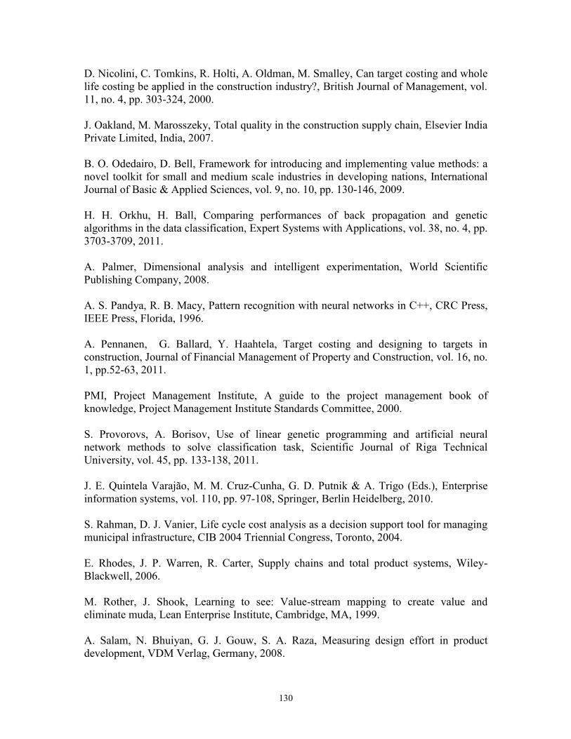
130
D. Nicolini, C. Tomkins, R. Holti, A. Oldman, M. Smalley, Can target costing and whole
life costing be applied in the construction industry?, British Journal of Management, vol.
11, no. 4, pp. 303-324, 2000.
J. Oakland, M. Marosszeky, Total quality in the construction supply chain, Elsevier India
Private Limited, India, 2007.
B. O. Odedairo, D. Bell, Framework for introducing and implementing value methods: a
novel toolkit for small and medium scale industries in developing nations, International
Journal of Basic & Applied Sciences, vol. 9, no. 10, pp. 130-146, 2009.
H. H. Orkhu, H. Ball, Comparing performances of back propagation and genetic
algorithms in the data classification, Expert Systems with Applications, vol. 38, no. 4, pp.
3703-3709, 2011.
A. Palmer, Dimensional analysis and intelligent experimentation, World Scientific
Publishing Company, 2008.
A. S. Pandya, R. B. Macy, Pattern recognition with neural networks in C++, CRC Press,
IEEE Press, Florida, 1996.
A. Pennanen, G. Ballard, Y. Haahtela, Target costing and designing to targets in
construction, Journal of Financial Management of Property and Construction, vol. 16, no.
1, pp.52-63, 2011.
PMI, Project Management Institute, A guide to the project management book of
knowledge, Project Management Institute Standards Committee, 2000.
S. Provorovs, A. Borisov, Use of linear genetic programming and artificial neural
network methods to solve classification task, Scientific Journal of Riga Technical
University, vol. 45, pp. 133-138, 2011.
J. E. Quintela Varajão, M. M. Cruz-Cunha, G. D. Putnik & A. Trigo (Eds.), Enterprise
information systems, vol. 110, pp. 97-108, Springer, Berlin Heidelberg, 2010.
S. Rahman, D. J. Vanier, Life cycle cost analysis as a decision support tool for managing
municipal infrastructure, CIB 2004 Triennial Congress, Toronto, 2004.
E. Rhodes, J. P. Warren, R. Carter, Supply chains and total product systems, Wiley-
Blackwell, 2006.
M. Rother, J. Shook, Learning to see: Value-stream mapping to create value and
eliminate muda, Lean Enterprise Institute, Cambridge, MA, 1999.
A. Salam, N. Bhuiyan, G. J. Gouw, S. A. Raza, Measuring design effort in product
development, VDM Verlag, Germany, 2008.
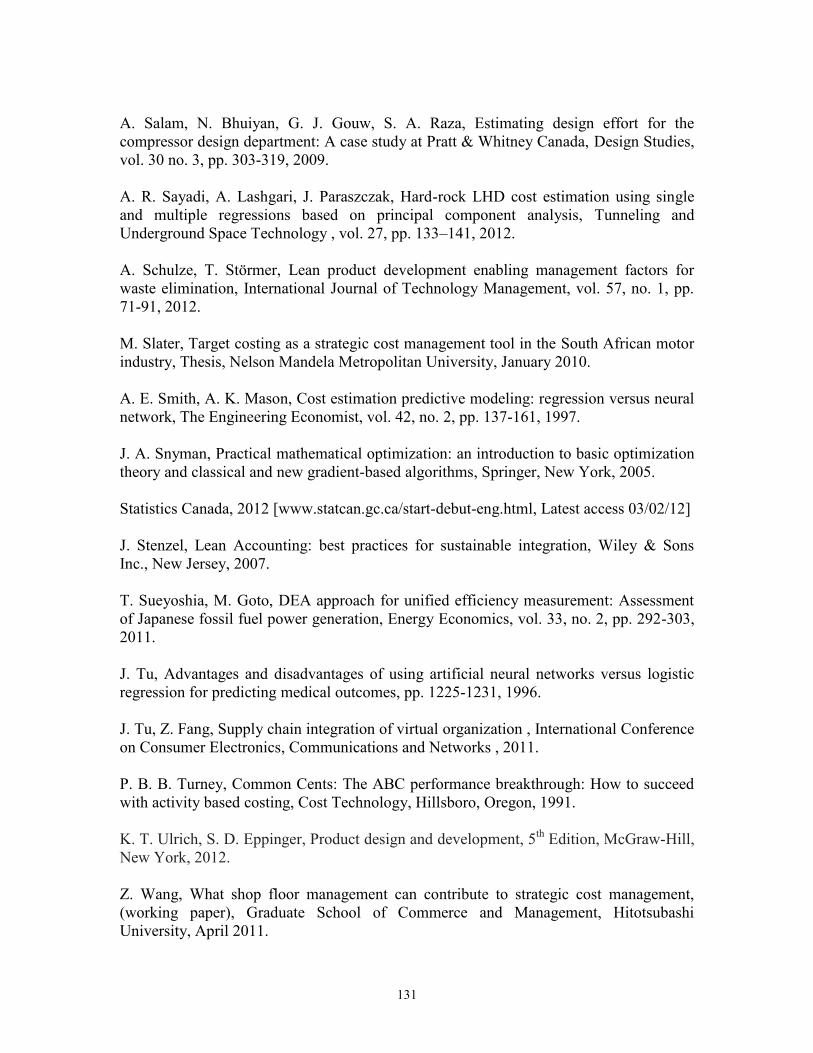
131
A. Salam, N. Bhuiyan, G. J. Gouw, S. A. Raza, Estimating design effort for the
compressor design department: A case study at Pratt & Whitney Canada, Design Studies,
vol. 30 no. 3, pp. 303-319, 2009.
A. R. Sayadi, A. Lashgari, J. Paraszczak, Hard-rock LHD cost estimation using single
and multiple regressions based on principal component analysis, Tunneling and
Underground Space Technology , vol. 27, pp. 133–141, 2012.
A. Schulze, T. Störmer, Lean product development enabling management factors for
waste elimination, International Journal of Technology Management, vol. 57, no. 1, pp.
71-91, 2012.
M. Slater, Target costing as a strategic cost management tool in the South African motor
industry, Thesis, Nelson Mandela Metropolitan University, January 2010.
A. E. Smith, A. K. Mason, Cost estimation predictive modeling: regression versus neural
network, The Engineering Economist, vol. 42, no. 2, pp. 137-161, 1997.
J. A. Snyman, Practical mathematical optimization: an introduction to basic optimization
theory and classical and new gradient-based algorithms, Springer, New York, 2005.
Statistics Canada, 2012 [www.statcan.gc.ca/start-debut-eng.html, Latest access 03/02/12]
J. Stenzel, Lean Accounting: best practices for sustainable integration, Wiley & Sons
Inc., New Jersey, 2007.
T. Sueyoshia, M. Goto, DEA approach for unified efficiency measurement: Assessment
of Japanese fossil fuel power generation, Energy Economics, vol. 33, no. 2, pp. 292-303,
2011.
J. Tu, Advantages and disadvantages of using artificial neural networks versus logistic
regression for predicting medical outcomes, pp. 1225-1231, 1996.
J. Tu, Z. Fang, Supply chain integration of virtual organization , International Conference
on Consumer Electronics, Communications and Networks , 2011.
P. B. B. Turney, Common Cents: The ABC performance breakthrough: How to succeed
with activity based costing, Cost Technology, Hillsboro, Oregon, 1991.
K. T. Ulrich, S. D. Eppinger, Product design and development, 5th
Edition, McGraw-Hill,
New York, 2012.
Z. Wang, What shop floor management can contribute to strategic cost management,
(working paper), Graduate School of Commerce and Management, Hitotsubashi
University, April 2011.
132
Y. Ward, A. Graves, A new cost management & accounting approach for lean
enterprises, (working paper), Irish Academy of Management Meeting Annual
Conference, Trinity College Dublin, September 2004.
Y. Ward, A. Graves, Lean performance measurement for aerospace management, vol. 1,
no.1, pp. 85-96, 2001.
S. Weisberg, Transformation: applied linear regression, Wiley-Interscience, Hoboken,
New Jersey, 2005.
J. P. Womack, D.T. Jones, Lean thinking: banish waste and create wealth in your
Corporation, Free Press, New York, 1996.
J. P. Womack, D.T. Jones, D. Roos, The machine that changed the world: based on the
Massachusetts Institute of Technology 5-million dollar 5-year study on the future of the
automobile, Rawson Associates, 1990.
S. Wright, The method of path coefficients, Annals of Math Stat, vol. 5, pp. 161-215,
1934.
H. Yazdifar, D. Askarany, A comparative study of the adoption and implementation of
target costing in the UK, Australia and New Zealand, International Journal of Production
Economics, vol.135,pp. 382-392, 2012.
M. Zangeneh, M. Omid, A. Akram, A comparative study between parametric and
artificial neural networks approaches for economical assessment of potato production in
Iran, Spanish Journal of Agricultural Research, vol. 9, no. 3, pp. 3061-3070, 2011.
I. J. Zbib, T. Rakotobe-Joel, R. Rigoli, Target costing: the key to supply chain excellence,
International Business & Economics Research Journal, vol. 2, no. 11, pp. 27-34, 2011.
J. Zhang, T. Li, X. Chen, L. Gu, Z. H.Wang, H. X. Cui, Prediction for air-bending
springback radius of sheet metal using back propagation neural network and micro
genetic algorithm, Materials Science Forum, vol. 704-705, pp. 1223-1230, 2012.
2011 BA Annual Report, 2011 Bombardier Annual Report
[bombardier.com/maintenance/2011Q4/BombardierAnnualReport_Dec2011_en.pdf,
Latest access 03/03/12]

133
APPENDIX A
134
Figure A.1: SPC chart for LR, 2 factors, sample A
Figure A.2: SPC chart for LR, 2 factors, sample B
60000
70000
80000
90000
100000
110000
120000
130000
60000 70000 80000 90000 100000 110000 120000 130000
Mas
ked
Co
st
Target Cost
60000
70000
80000
90000
100000
110000
120000
130000
60000 70000 80000 90000 100000 110000 120000 130000
Mas
ked
Co
st
Target Cost
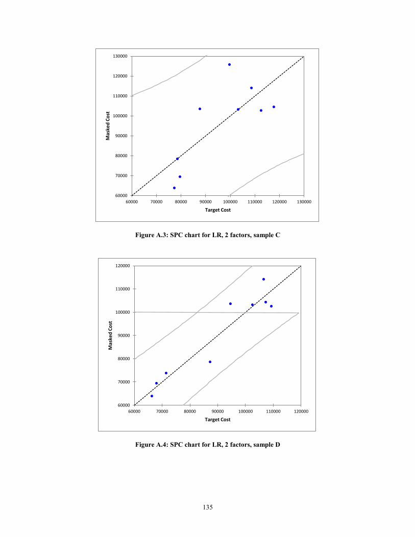
135
Figure A.3: SPC chart for LR, 2 factors, sample C
Figure A.4: SPC chart for LR, 2 factors, sample D
60000
70000
80000
90000
100000
110000
120000
130000
60000 70000 80000 90000 100000 110000 120000 130000
Mas
ked
Co
st
Target Cost
60000
70000
80000
90000
100000
110000
120000
60000 70000 80000 90000 100000 110000 120000
Mas
ked
Co
st
Target Cost

136
Figure A.5: SPC chart for LR, 2 factors, sample E
Figure A.6: SPC chart for LR, 2 factors, sample F
60000
70000
80000
90000
100000
110000
120000
130000
60000 70000 80000 90000 100000 110000 120000 130000
Mas
ked
Co
st
Target Cost
60000
70000
80000
90000
100000
110000
120000
130000
60000 70000 80000 90000 100000 110000 120000 130000
Mas
ked
Co
st
Target Cost
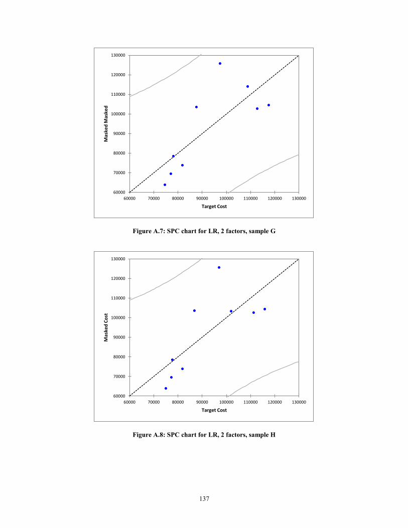
137
Figure A.7: SPC chart for LR, 2 factors, sample G
Figure A.8: SPC chart for LR, 2 factors, sample H
60000
70000
80000
90000
100000
110000
120000
130000
60000 70000 80000 90000 100000 110000 120000 130000
Mas
ked
Mas
ked
Target Cost
60000
70000
80000
90000
100000
110000
120000
130000
60000 70000 80000 90000 100000 110000 120000 130000
Mas
ked
Co
st
Target Cost
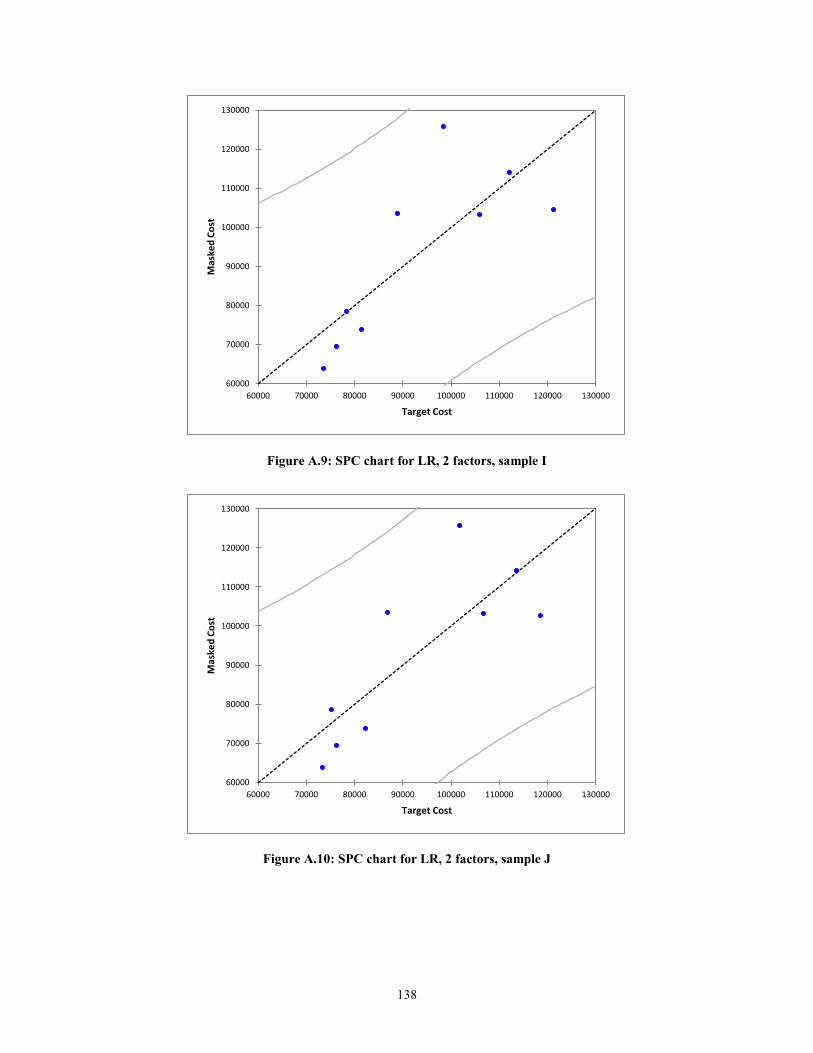
138
Figure A.9: SPC chart for LR, 2 factors, sample I
Figure A.10: SPC chart for LR, 2 factors, sample J
60000
70000
80000
90000
100000
110000
120000
130000
60000 70000 80000 90000 100000 110000 120000 130000
Mas
ked
Co
st
Target Cost
60000
70000
80000
90000
100000
110000
120000
130000
60000 70000 80000 90000 100000 110000 120000 130000
Mas
ked
Co
st
Target Cost

139
APPENDIX B
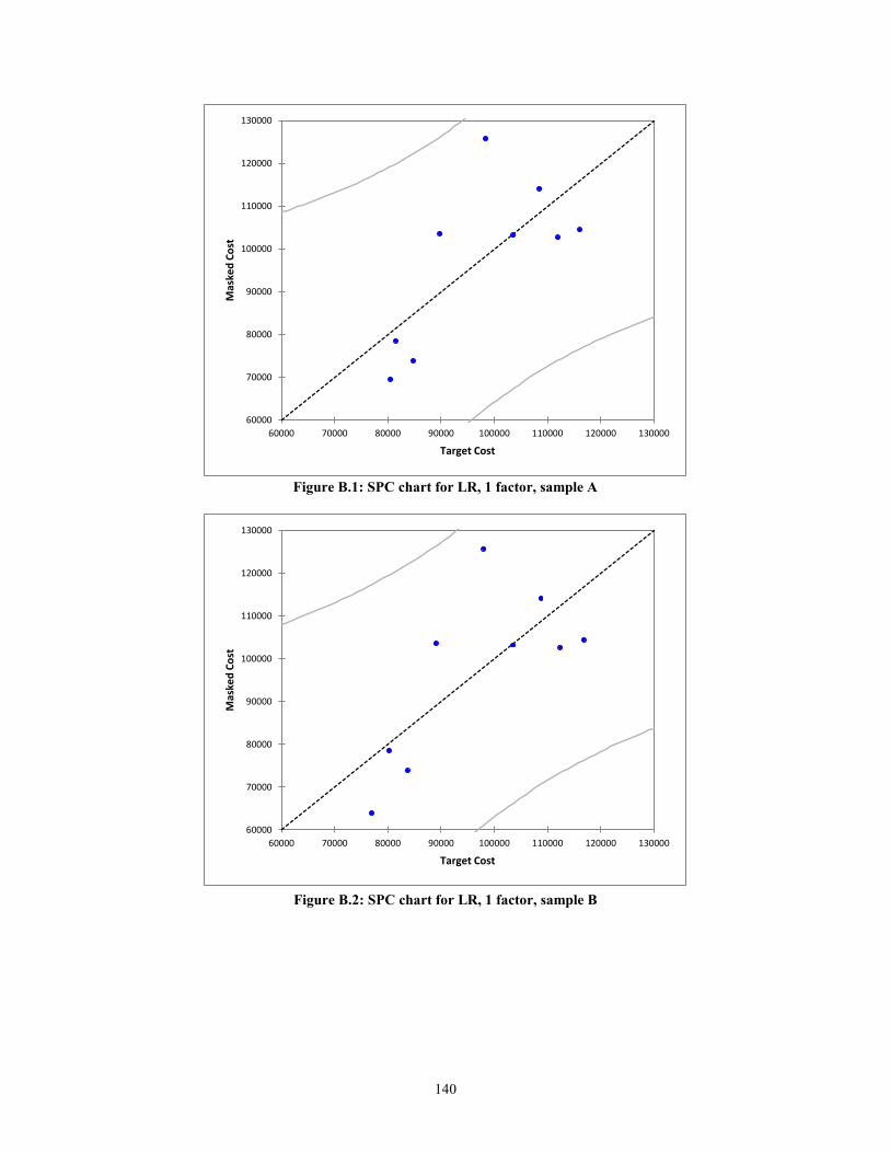
140
Figure B.1: SPC chart for LR, 1 factor, sample A
Figure B.2: SPC chart for LR, 1 factor, sample B
60000
70000
80000
90000
100000
110000
120000
130000
60000 70000 80000 90000 100000 110000 120000 130000
Mas
ked
Co
st
Target Cost
60000
70000
80000
90000
100000
110000
120000
130000
60000 70000 80000 90000 100000 110000 120000 130000
Mas
ked
Co
st
Target Cost

141
Figure B.3: SPC chart for LR, 1 factor, sample C
Figure B.4: SPC chart for LR, 1 factor, sample D
60000
70000
80000
90000
100000
110000
120000
130000
60000 70000 80000 90000 100000 110000 120000 130000
Mas
ked
Co
st
Target Cost
60000
70000
80000
90000
100000
110000
120000
60000 70000 80000 90000 100000 110000 120000
Mas
ked
Co
st
Target Cost

142
Figure B.5: SPC chart for LR, 1 factor, sample E
Figure B.6: SPC chart for LR, 1 factor, sample F
60000
70000
80000
90000
100000
110000
120000
130000
60000 70000 80000 90000 100000 110000 120000 130000
Mas
ked
Co
st
Target Cost
60000
70000
80000
90000
100000
110000
120000
130000
60000 70000 80000 90000 100000 110000 120000 130000
Mas
ked
Cp
st
Target Cost
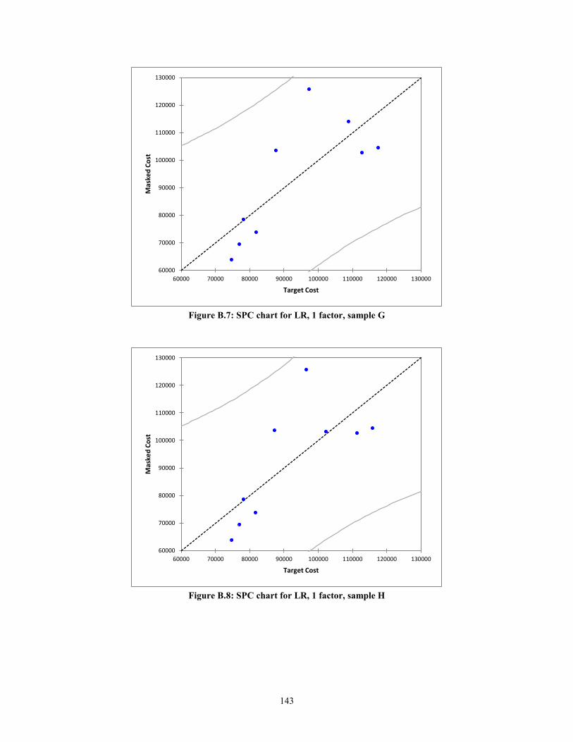
143
Figure B.7: SPC chart for LR, 1 factor, sample G
Figure B.8: SPC chart for LR, 1 factor, sample H
60000
70000
80000
90000
100000
110000
120000
130000
60000 70000 80000 90000 100000 110000 120000 130000
Mas
ked
Co
st
Target Cost
60000
70000
80000
90000
100000
110000
120000
130000
60000 70000 80000 90000 100000 110000 120000 130000
Mas
ked
Co
st
Target Cost
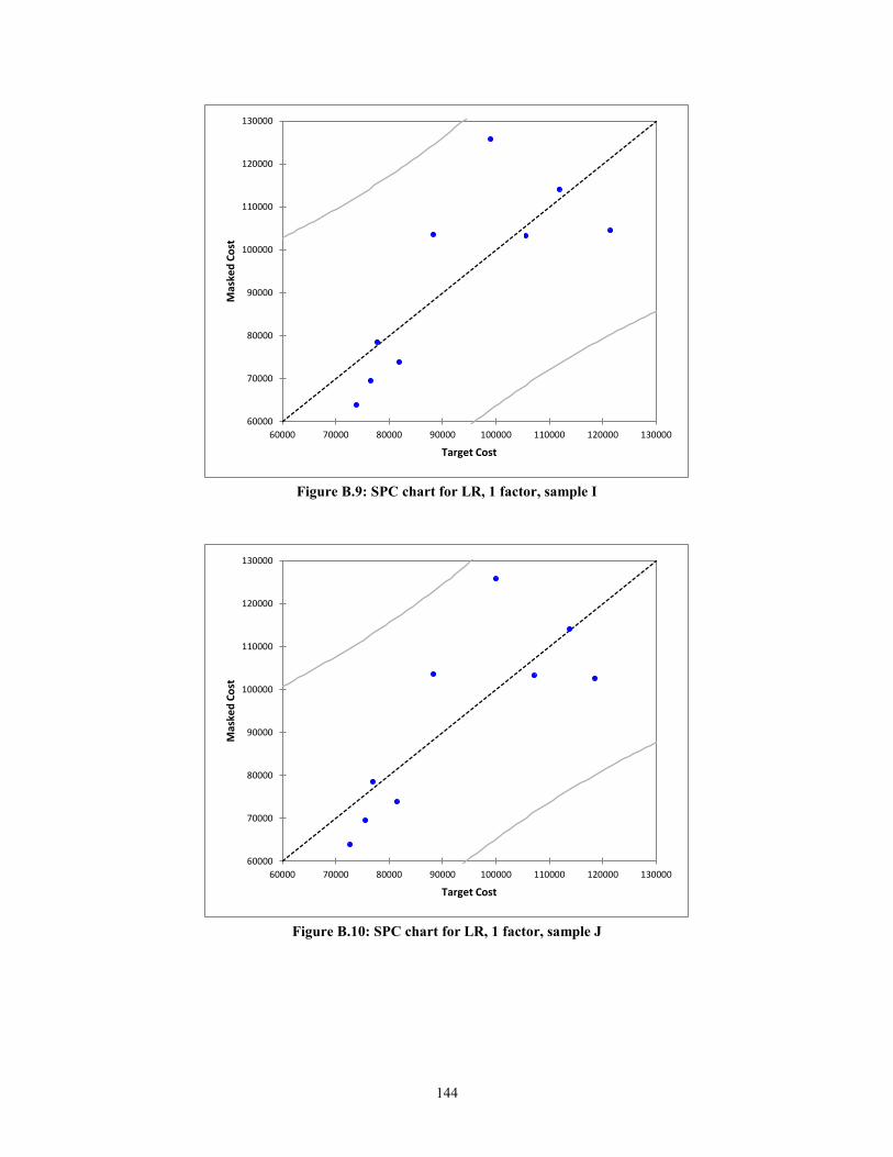
144
Figure B.9: SPC chart for LR, 1 factor, sample I
Figure B.10: SPC chart for LR, 1 factor, sample J
60000
70000
80000
90000
100000
110000
120000
130000
60000 70000 80000 90000 100000 110000 120000 130000
Mas
ked
Co
st
Target Cost
60000
70000
80000
90000
100000
110000
120000
130000
60000 70000 80000 90000 100000 110000 120000 130000
Mas
ked
Co
st
Target Cost

145
APPENDIX C
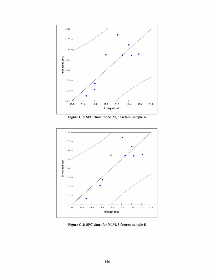
146
Figure C.1: SPC chart for NLM, 3 factors, sample A
Figure C.2: SPC chart for NLM, 3 factors, sample B
11.1
11.2
11.3
11.4
11.5
11.6
11.7
11.8
11.1 11.2 11.3 11.4 11.5 11.6 11.7 11.8
ln m
aske
d c
ost
ln target cost
11
11.1
11.2
11.3
11.4
11.5
11.6
11.7
11.8
11 11.1 11.2 11.3 11.4 11.5 11.6 11.7 11.8
ln m
aske
d c
ost
ln taget cost
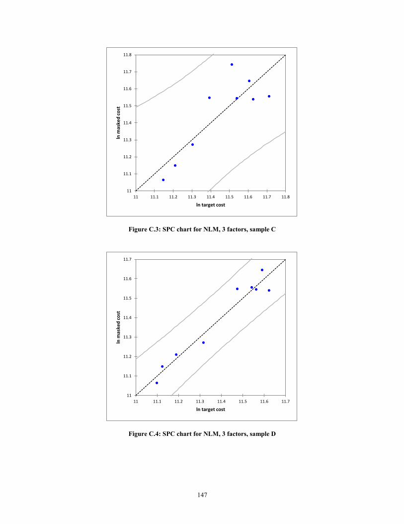
147
Figure C.3: SPC chart for NLM, 3 factors, sample C
Figure C.4: SPC chart for NLM, 3 factors, sample D
11
11.1
11.2
11.3
11.4
11.5
11.6
11.7
11.8
11 11.1 11.2 11.3 11.4 11.5 11.6 11.7 11.8
ln m
aske
d c
ost
ln target cost
11
11.1
11.2
11.3
11.4
11.5
11.6
11.7
11 11.1 11.2 11.3 11.4 11.5 11.6 11.7
ln m
aske
d c
ost
ln target cost
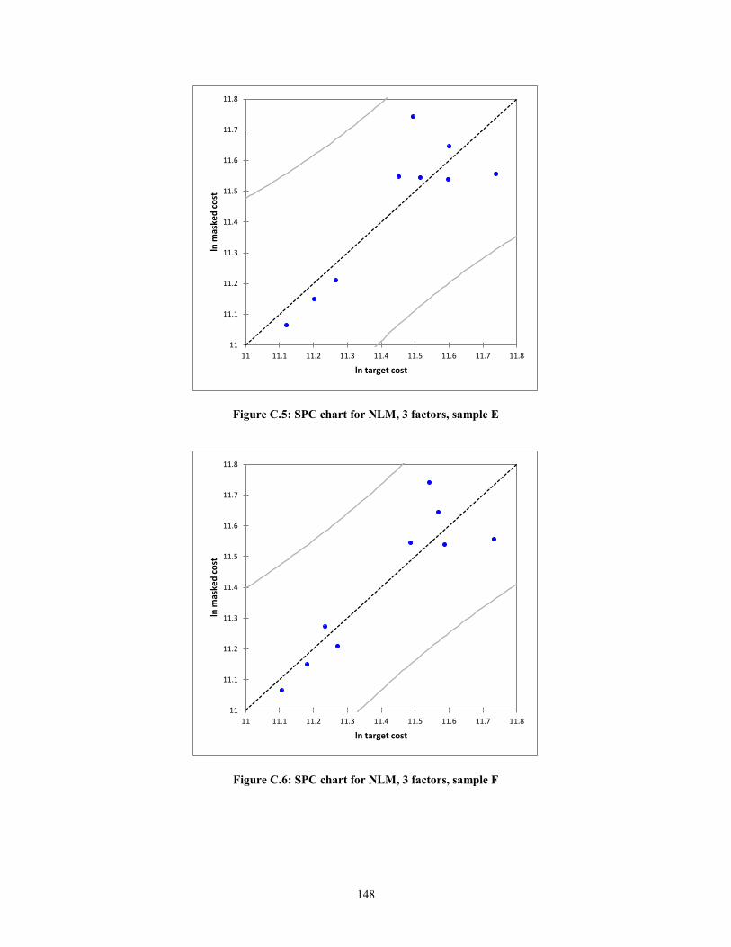
148
Figure C.5: SPC chart for NLM, 3 factors, sample E
Figure C.6: SPC chart for NLM, 3 factors, sample F
11
11.1
11.2
11.3
11.4
11.5
11.6
11.7
11.8
11 11.1 11.2 11.3 11.4 11.5 11.6 11.7 11.8
ln m
aske
d c
ost
ln target cost
11
11.1
11.2
11.3
11.4
11.5
11.6
11.7
11.8
11 11.1 11.2 11.3 11.4 11.5 11.6 11.7 11.8
ln m
aske
d c
ost
ln target cost
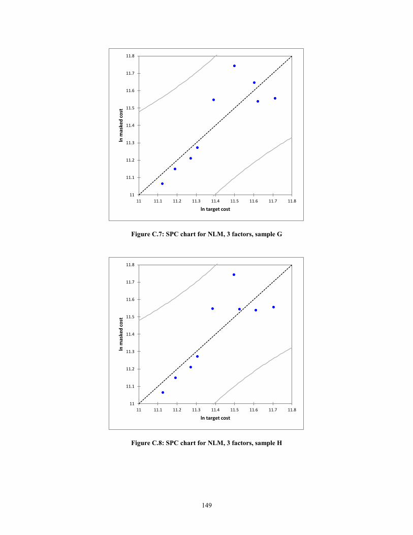
149
Figure C.7: SPC chart for NLM, 3 factors, sample G
Figure C.8: SPC chart for NLM, 3 factors, sample H
11
11.1
11.2
11.3
11.4
11.5
11.6
11.7
11.8
11 11.1 11.2 11.3 11.4 11.5 11.6 11.7 11.8
ln m
aske
d c
ost
ln target cost
11
11.1
11.2
11.3
11.4
11.5
11.6
11.7
11.8
11 11.1 11.2 11.3 11.4 11.5 11.6 11.7 11.8
ln m
aske
d c
ost
ln target cost
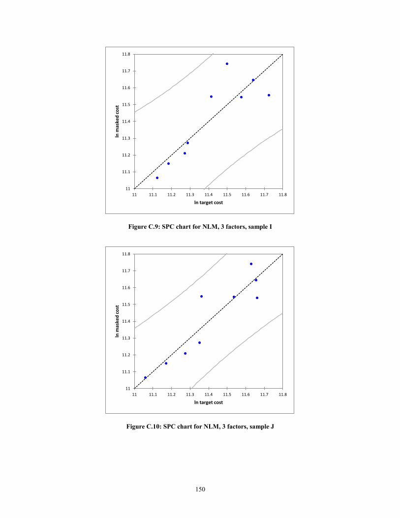
150
Figure C.9: SPC chart for NLM, 3 factors, sample I
Figure C.10: SPC chart for NLM, 3 factors, sample J
11
11.1
11.2
11.3
11.4
11.5
11.6
11.7
11.8
11 11.1 11.2 11.3 11.4 11.5 11.6 11.7 11.8
ln m
aske
d c
ost
ln target cost
11
11.1
11.2
11.3
11.4
11.5
11.6
11.7
11.8
11 11.1 11.2 11.3 11.4 11.5 11.6 11.7 11.8
ln m
aske
d c
ost
ln target cost

151
APPENDIX D
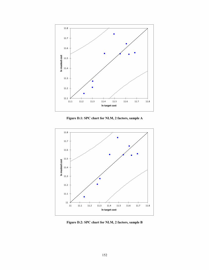
152
Figure D.1: SPC chart for NLM, 2 factors, sample A
Figure D.2: SPC chart for NLM, 2 factors, sample B
11.1
11.2
11.3
11.4
11.5
11.6
11.7
11.8
11.1 11.2 11.3 11.4 11.5 11.6 11.7 11.8
ln m
aske
d c
ost
ln target cost
11
11.1
11.2
11.3
11.4
11.5
11.6
11.7
11.8
11 11.1 11.2 11.3 11.4 11.5 11.6 11.7 11.8
ln m
aske
d c
ost
ln target cost

153
Figure D.3: SPC chart for NLM, 2 factors, sample C
Figure D.4: SPC chart for NLM, 2 factors, sample D
11
11.1
11.2
11.3
11.4
11.5
11.6
11.7
11.8
11 11.1 11.2 11.3 11.4 11.5 11.6 11.7 11.8
ln m
aske
d c
ost
ln target cost
11
11.1
11.2
11.3
11.4
11.5
11.6
11.7
11 11.1 11.2 11.3 11.4 11.5 11.6 11.7
ln m
aske
d c
ost
ln target cost

154
Figure D.5: SPC chart for NLM, 2 factors, sample E
Figure D.6: SPC chart for NLM, 2 factors, sample F
11
11.1
11.2
11.3
11.4
11.5
11.6
11.7
11.8
11 11.1 11.2 11.3 11.4 11.5 11.6 11.7 11.8
ln m
aske
d c
ost
ln target cost
11
11.1
11.2
11.3
11.4
11.5
11.6
11.7
11.8
11 11.1 11.2 11.3 11.4 11.5 11.6 11.7 11.8
ln m
aske
d c
ost
ln target cost
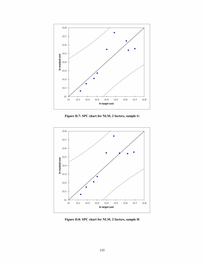
155
Figure D.7: SPC chart for NLM, 2 factors, sample G
Figure D.8: SPC chart for NLM, 2 factors, sample H
11
11.1
11.2
11.3
11.4
11.5
11.6
11.7
11.8
11 11.1 11.2 11.3 11.4 11.5 11.6 11.7 11.8
ln m
aske
d c
ost
ln target cost
11
11.1
11.2
11.3
11.4
11.5
11.6
11.7
11.8
11 11.1 11.2 11.3 11.4 11.5 11.6 11.7 11.8
ln m
aske
d c
ost
ln target cost
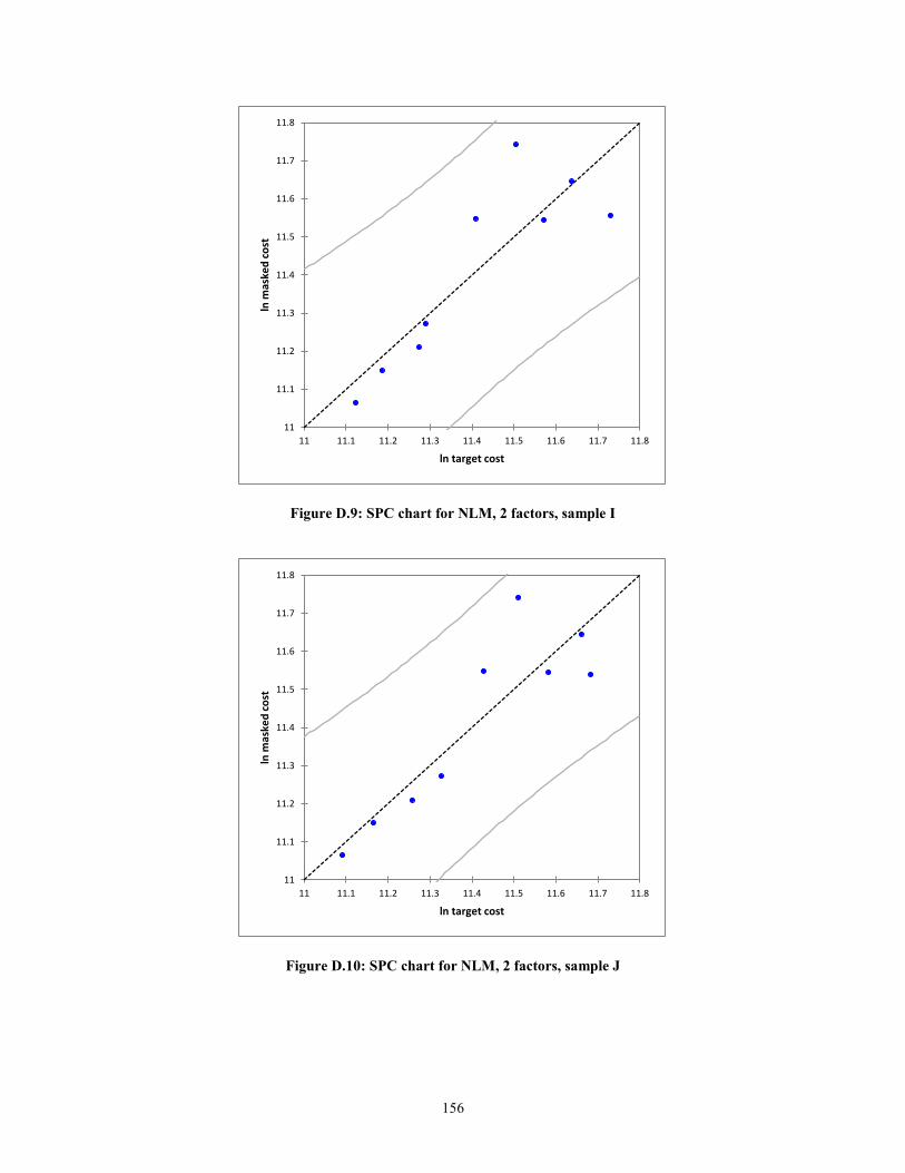
156
Figure D.9: SPC chart for NLM, 2 factors, sample I
Figure D.10: SPC chart for NLM, 2 factors, sample J
11
11.1
11.2
11.3
11.4
11.5
11.6
11.7
11.8
11 11.1 11.2 11.3 11.4 11.5 11.6 11.7 11.8
ln m
aske
d c
ost
ln target cost
11
11.1
11.2
11.3
11.4
11.5
11.6
11.7
11.8
11 11.1 11.2 11.3 11.4 11.5 11.6 11.7 11.8
ln m
aske
d c
ost
ln target cost

157
APPENDIX E
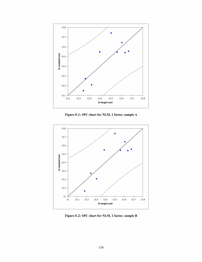
158
Figure E.1: SPC chart for NLM, 1 factor, sample A
Figure E.2: SPC chart for NLM, 1 factor, sample B
11.1
11.2
11.3
11.4
11.5
11.6
11.7
11.8
11.1 11.2 11.3 11.4 11.5 11.6 11.7 11.8
ln m
aske
d c
ost
ln target cost
11
11.1
11.2
11.3
11.4
11.5
11.6
11.7
11.8
11 11.1 11.2 11.3 11.4 11.5 11.6 11.7 11.8
ln m
aske
d c
ost
ln target cost
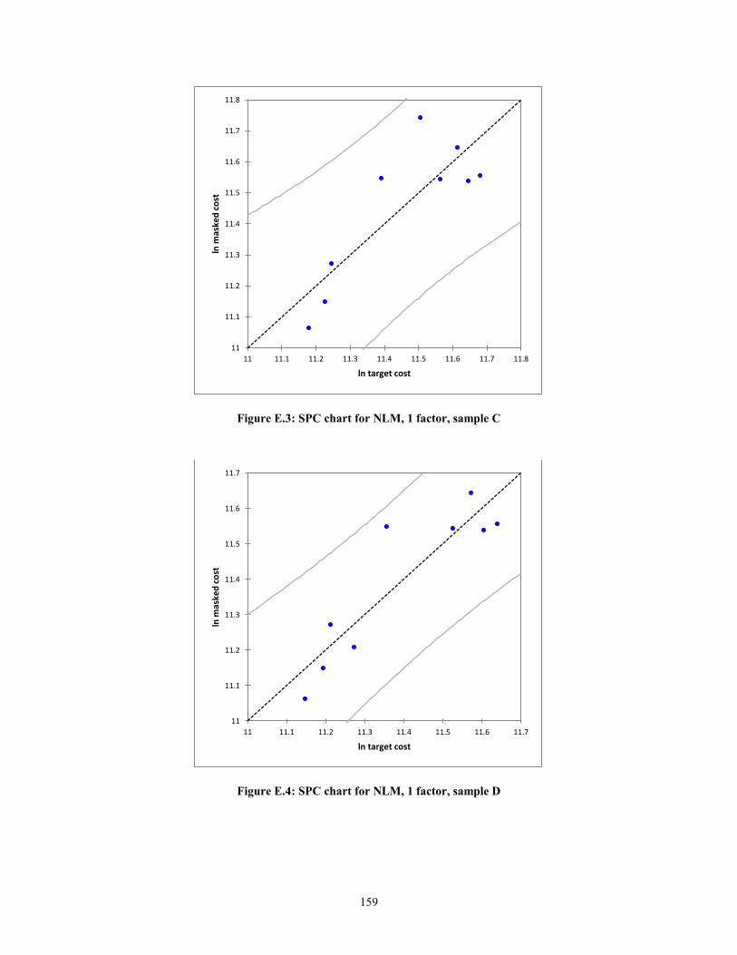
159
Figure E.3: SPC chart for NLM, 1 factor, sample C
Figure E.4: SPC chart for NLM, 1 factor, sample D
11
11.1
11.2
11.3
11.4
11.5
11.6
11.7
11.8
11 11.1 11.2 11.3 11.4 11.5 11.6 11.7 11.8
ln m
aske
d c
ost
ln target cost
11
11.1
11.2
11.3
11.4
11.5
11.6
11.7
11 11.1 11.2 11.3 11.4 11.5 11.6 11.7
ln m
aske
d c
ost
ln target cost

160
Figure E.5: SPC chart for NLM, 1 factor, sample E
Figure E.6: SPC chart for NLM, 1 factor, sample F
11
11.1
11.2
11.3
11.4
11.5
11.6
11.7
11.8
11 11.1 11.2 11.3 11.4 11.5 11.6 11.7 11.8
ln m
aske
d c
ost
ln target cost
11
11.1
11.2
11.3
11.4
11.5
11.6
11.7
11.8
11 11.1 11.2 11.3 11.4 11.5 11.6 11.7 11.8
ln m
aske
d c
ost
ln target cost
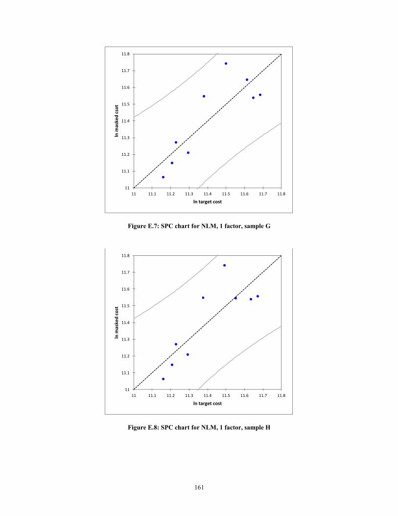
161
Figure E.7: SPC chart for NLM, 1 factor, sample G
Figure E.8: SPC chart for NLM, 1 factor, sample H
11
11.1
11.2
11.3
11.4
11.5
11.6
11.7
11.8
11 11.1 11.2 11.3 11.4 11.5 11.6 11.7 11.8
ln m
aske
d c
sot
ln target cost
11
11.1
11.2
11.3
11.4
11.5
11.6
11.7
11.8
11 11.1 11.2 11.3 11.4 11.5 11.6 11.7 11.8
ln m
aske
d c
ost
ln target cost

162
Figure E.9: SPC chart for NLM, 1 factor, sample I
Figure E.10: SPC chart for NLM, 1 factor, sample J
11
11.1
11.2
11.3
11.4
11.5
11.6
11.7
11.8
11 11.1 11.2 11.3 11.4 11.5 11.6 11.7 11.8
ln m
aske
d c
ost
ln target cost
11
11.1
11.2
11.3
11.4
11.5
11.6
11.7
11.8
11 11.1 11.2 11.3 11.4 11.5 11.6 11.7 11.8
ln m
aske
d c
ost
ln target cost