Learning an Optimization Algorithm through

Human Design Iterations

Thurston Sexton∗1 and Max Yi Ren†1

1Department of Mechanical Engineering, Arizona State University

April 28, 2017

Abstract

Solving optimal design problems through crowdsourcing faces adilemma: On one hand, human beings have been shown to be moreeffective than algorithms at searching for good solutions of certain real-world problems with high-dimensional or discrete solution spaces; onthe other hand, the cost of setting up crowdsourcing environments, theuncertainty in the crowd’s domain-specific competence, and the lackof commitment of the crowd, all contribute to the lack of real-worldapplication of design crowdsourcing. We are thus motivated to investi-gate a solution-searching mechanism where an optimization algorithmis tuned based on human demonstrations on solution searching, sothat the search can be continued after human participants abandonthe problem. To do so, we model the iterative search process as aBayesian Optimization (BO) algorithm, and propose an inverse BO(IBO) algorithm to find the maximum likelihood estimators of the BOparameters based on human solutions. We show through a vehicle de-sign and control problem that the search performance of BO can beimproved by recovering its parameters based on an effective humansearch. Thus, IBO has the potential to improve the success rate of de-sign crowdsourcing activities, by requiring only good search strategiesinstead of good solutions from the crowd.

∗tbsexton@asu.edu†yiren@asu.edu

1

arX

iv:1

608.

0698

4v4

[cs

.LG

] 2

6 A

pr 2

017

1 Introduction

1.1 Challenges and opportunities for design crowdsourcing

Optimal design problems often have large solution spaces and highly non-convex objectives and constraints, inhibiting effective solution searchingthrough existing optimization algorithms. Some of these problems, however,have been quite successfully (yet heuristically) solved by human beings. No-table examples include protein folding [1, 2], RNA synthesis [3, 4], genomesequence alignment [5], robot trajectory planning [6], and others [7–9].The superior performance of some human beings at solving these problemsdemonstrates the advantages of human intelligence, which are supported bycognitive science and neuroscience findings [10] (see discussion in Sec. 5.1).However, despite a handful of success stories, applications of crowdsourc-ing to real-world design problems have yet to overcome several practicalbarriers. The cost of setting up problem-dependent crowdsourcing environ-ments, the lack of commitment from crowd members, and uncertainty indomain-specific crowd competence have all contributed to its lack of adop-tion, while the growing availability of computation resources often makesstraight-forward optimization or brute-force search a more convenient ap-proach.

Our earlier study [8] highlighted these challenges for design crowdsourc-ing: We gamified a vehicle design and control problem (called the “ecoRacer”problem in what follows) where the objective is to complete a track withthe minimal energy consumption within a time limit, by finding the optimalfinal drive ratio of the vehicle and the control policy for acceleration andregenerative braking. The game was broadcast on social media and receivedmore than 2000 plays from 124 unique players within the first month. Re-sults showed that (1) the marginal improvement in average game score ofthe crowd over an algorithm does not necessarily justify the high cost fordeveloping crowdsourcing games, and (2) only a few players were committedto the search for more than 50 iterations, and still fewer can outperform thecomputer-found solution at all (see summary in Fig. 1).

Nonetheless, human search results displayed a significantly different searchpattern than that of the algorithm. In particular, quite a few players showedrapid early improvement in performance, beyond the average performanceof the computer, before they quit the game without reaching a solutionclose to the theoretical optimum. This observation is consistent with ex-isting research (see, for example, [2] on a human-designed protein foldingalgorithm having a short-term advantage over a standard algorithm), and

2

Figure 1: (a) Summary of player participation and performance (b) Resultsfrom the game showed while most players failed to outperform the BayesianOptimization algorithm, some of them can identify good solutions early on.Image is reproduced from [8,11].

3

suggests that while few people care to actually find the “best solution”,their early demonstrations on how they search for a better solution may stillbe valuable. Specifically, we hypothesize that if a computer algorithm canbe tuned to mimic these demonstrations, it can serve as a replacement tohuman solvers in their absence, to search in an effective way without everabandoning the problem.

1.2 Learning to search

This paper aims to test the above hypothesis. We model a human solver’ssearch behavior through a Bayesian Optimization algorithm (BO, also knownas Efficient Global Optimization) [12, 13]. The algorithm iterates betweentwo steps: (1) Estimating the shape of the problem space, based on previoussolutions and corresponding performances, using a Gaussian Process (GP)model [14], and (2) creating a new solution based on this estimate (detailsin Sec. 2). While BO is not provably the underlying mechanism humansuse, we hypothesize that the algorithm can be tuned to mimic the resultsof successful human search strategies, specifically in comparison with otherpopular gradient- and non-gradient-based optimization algorithms. The keyassumption in modeling human search behavior through BO is the use ofa GP to account for human beings’ learning of input-output relationships(or called “function learning” in psychology). This assumption is supportedby various findings: In a recent review of function-learning models, Christo-pher et al. [15] showed that the two major schools of models, i.e., rules- andsimilarity-based, can be unified through a Gaussian Process1. As discussedin Wilson et al. [16], the evidence that Occam’s Razor plays an importantrole in human prediction also suggests that GP is an appropriate modelfor function learning, as GP reduces model complexity by construction [17].Empirically, Borji et al. [18] showed that BO, with the use of GP, has theclosest convergence performance to human searches when applied to 1Doptimization problems. In fact, many higher-dimensional problems that hu-man beings naturally solve, such as locomotion planning, have also beensuccessfully solved through the use of GP [19–22].

Under this modeling assumption, we investigate how BO parameterscan be estimated for the algorithm to best match human solver’s searchtrajectory, i.e., the sequence of solution-performance pairs. To this end, we

1To be more accurate, the discussion in [15] is for function learning with continuousvariables. While our case study involves discrete variables (acceleration and braking sig-nals), the dimension reduction process converts these variables to continuous ones. SeeSec. 4.

4

introduce an Inverse BO (IBO) algorithm to derive the maximum likelihoodestimators for BO parameters, and discuss challenges in its implementation(see Sec. 3). Validation of the IBO algorithm takes two steps. We first use asimulation study to show that IBO can successfully estimate BO parametersused in generating a search trajectory (Sec. 3.2). We then show through theecoRacer problem that the search performance of BO can be improved whenits parameters are modified based on observing an effective human searchand implementing IBO (Sec. 4). The results provide evidence that IBOcan accelerate a search using only good search strategies without needing alarge number of good human solutions. Thus, incorporating IBO in designcrowdsourcing may lower the requirement on crowd commitment and soincrease its chance of success. Limitations and their potential relaxations ofthe current IBO implementation will be discussed in depth in Sec. 5.

1.3 Related work

It is important to note that the focus of this paper is on the design ofoptimization algorithms aided by human demonstrations, rather than thederivation of qualitative explanations of the strengths and limitations of hu-man design strategies. There have been numerous studies from the lattercategory in recent years (see [23–28] for example). This paper is also distin-guished from studies that propose human-inspired optimization algorithms(see [29–31] for example), in that the learning of the optimization algo-rithm in our case is conducted by another algorithm, rather than by humanresearchers. From this aspect, our study is related to studies in learning-to-learn [32] where algorithms (e.g., for gradient-based optimization [33] andoptimal control [34]) are tuned and controlled by a higher-level algorithm. Insuch work, however, the algorithms are often improved purely computation-ally through reinforcement learning by solving similar problems repeatedly.Due to the use of human demonstrations, our paper is also related to inversereinforcement learning (see discussion in Subsec. 5.2), where human controlstrategies are used for defining and finding optimal control strategies.

2 Preliminaries on Bayesian Optimization

This section provides some background knowledge on BO to facilitate thediscussion on IBO in Sec. 3.

5

2.1 Terminologies and notations

Let an optimization problem be minx∈X f(x) where X ⊆ Rp is the solutionspace. A search trajectory with K iterations can be represented by hK :=<XK , fK >, where XK and fK represent the collection of K samples in Xand their objective values, respectively. h0 :=< X0, f0 > represents aninitial exploration set with K0 samples. Human strategy is representedby algorithmic parameters λ that govern the search behavior: During thesearch, each new solution xk+1 (for k = 0, · · · ,K − 1) is determined byhk :=< Xk, fk > and λ through maximizing a merit function with respectto x: xk+1 = argmaxx∈XQ(x;hk,λ). The functional forms of the meritfunction Q(x) will be introduced in Subsecs. 2.2 and 3. We also defineΛ := diag(λ) and its estimator as Λ := diag(λ).

2.2 The BO algorithm

We briefly review the BO algorithm, to explain how each new sample x isdrawn based on the merit function Q(x), itself defined by previous sam-ples. Knowing this procedure is necessary for understanding the inverse BOalgorithm, where we estimate the most likely BO parameters for a giventrajectory of samples.

BO contains two major steps in each iteration: For a collection of sam-ples of a black-box function, a Gaussian Process (GP) model is updated;the merit function is then formulated based on the GP model, and the nextsample is chosen by maximizing the merit. Model update: It first up-dates a Gaussian Process (GP) model to predict objective values, based oncurrent observations hk and Gaussian parameters λ. Without consideringrandom noise in evaluating the objective, the GP model can be derived as

f(x;hk,λ) = b + rTR−1(fk − b), where b = 1T R−1fk1T R−11

, r is a column vector

with elements ri = exp(−(x− xi)

TΛ(x− xi))

for i = 1, · · · , k, R is a sym-metric matrix with Rij = exp

(−(xi − xj)

TΛ(xi − xj))

for i, j = 1, · · · , k,and 1 is a column vector with ones. Without prior knowledge, the Maxi-mum Likelihood Estimator (MLE) of λ for the GP model can be derived bysolving

λGP = argminλ log(σk|R|12 ), (1)

where σ2 = (fk − 1b)TR−1(fk − 1b)/n is the MLE of the GP variance.Sampling the solution space: The second step is to determine the nextsample using the GP model. A common sampling strategy is to pick the newsolution in X that maximizes the expected improvement from the currentbest objective value fmin := min fk (assuming a minimization problem):

6

QEI(x;hk,λ) = (fmin− f)Φ(fmin−f

σ

)+σφ

(fmin−f

σ

). Here Φ(·) and φ(·) are

the cumulative distribution function and probability density function of thestandard normal distribution, respectively. The new sample is thus obtainedby solving

xk+1 = argmaxx∈XQEI(x;hk,λ). (2)

Fig. 2 demonstrates four iterations of BO in optimizing a 1D function, withthe GP model and the expected improvement function updated in eachiteration. Note that similar to human searching behavior, BO is a stochasticprocess: First, the choice of the new design is stochastic, with better designsbeing more probable to be chosen2; and secondly, the initial exploration h0can be stochastic when it is modeled by a random sampling scheme, e.g.,Latin Hypercube sampling (LHS, see [12] for details).

3 Inverse BO

We consider human solution search to consist two stages: A few exploratorysearches are first conducted to acquire a preliminary understanding of theproblem, before the execution of BO follows. For example, a player mayspend a few trials to get familiar with a new game, before thinking aboutstrategies to improve his score. IBO minimizes the sum of two costs cor-responding to the exploration and BO stages, respectively. By doing so, itfinds the most likely explanation of the underlying search strategy.

Specifically, IBO estimates λ, along with the size of the initial explo-ration set K0, given the trajectory hK . To do so, we introduce and min-imize a cost function consisting of the exploration cost for h0, denoted asLINI , and the BO cost for the rest of hK , denoted as LBO. We defineLINI := − log (Dp(X0)) where p(X0) is the joint probability of the explo-ration set and D := |X | is the size of the solution space; and LBO :=− log (Dp(hK − h0|h0)) = −

∑K−1k=0 log (Dp(xk+1|hk)) where p(xk+1|hk) is

the density for choosing xk+1 conditioned on hk. Here log(·) stands fornatural logarithm.

The derivation of LINI and LBO are as follows: To calculate LINI ,we assume that each new sample during the exploration phase, xi for i =1, · · · ,K0, tends to maximize its minimum Euclidean distance d(xi,X<i) toprevious samples X<i, this is referred to as the max-min sampling scheme

2Numerically, this is because optimizing the non-convex function QEI requires a nestedglobal optimization routine, such as Genetic Algorithm (GA), CMA-ES [35], DIRECT [36],and BARON [37]. Some implementations of these, e.g., GA and CMA-ES, can be stochas-tic.

7

Figure 2: Four iterations of BO on a 1D function. Obj: The objective func-tion. GP: Gaussian Process model. EI: Expected Improvement function.Image is modified from [11].

8

in what follows. Let the joint probability of the exploration set be p(X0) =p(x1)p(x2|x1) · · · p(xK0 |X<K0) and each conditional probability follow a Boltz-mann distribution: p(xi|X<i) = exp (αINId(xi,X<i)) /ZINI(xi, αINI). Herethe scalar αINI represents how strictly each sample from X0 follows the max-min sampling scheme, and ZINI(xi, αINI) =

∫x∈X exp (αINId(x,X<i)) dx is

a partition function that ensures that∫X p(xi|X<i)dx = 1. Note that the

first sample in the exploration set is considered to be uniformly drawn, andthus its contribution to the cost (a constant) can be omitted.

To calculate LBO, the conditional probability density of sampling x ∈ Xbased on current hk can be similarly modeled as a Boltzmann distribution:

p(x|hk) = exp (αBOQEI(x;hk,λ)) /ZBO(hk,λ, αBO), (3)

where ZBO(hk,λ, αBO) =∫x∈X exp (αBOQEI(x;hk,λ)) dx is also a partition

function. The parameter αBO plays a similar role to αINI . For simplicity,we define li := − log (Dp(xi|X<i)) and lk := − log (Dp(xk+1|hk)), so thatLINI =

∑K0i=1 li and LBO =

∑K−1k=0 lk. A lower value of l or l represents

higher probability density of the current sample to be drawn by max-minsampling or BO, respectively, and a zero indicates that the sample can beconsidered as uniformly drawn.

IBO solves the following problem to derive λ.

minαINI ,αBO,λ,K0

L := LINI + LBO (4)

Note that to find the optimal K0 for any given αINI , αBO, and λ, onecan first calculate the optimal li and lk for i, k = 2, · · · ,K, with respect toαINI , αBO, and λ, and then scan K0 = 2, · · · ,K to find the lowest valueof LINI + LBO. The scan starts at K0 = 2 because it is not meaningful toinitialize BO with a single sample.

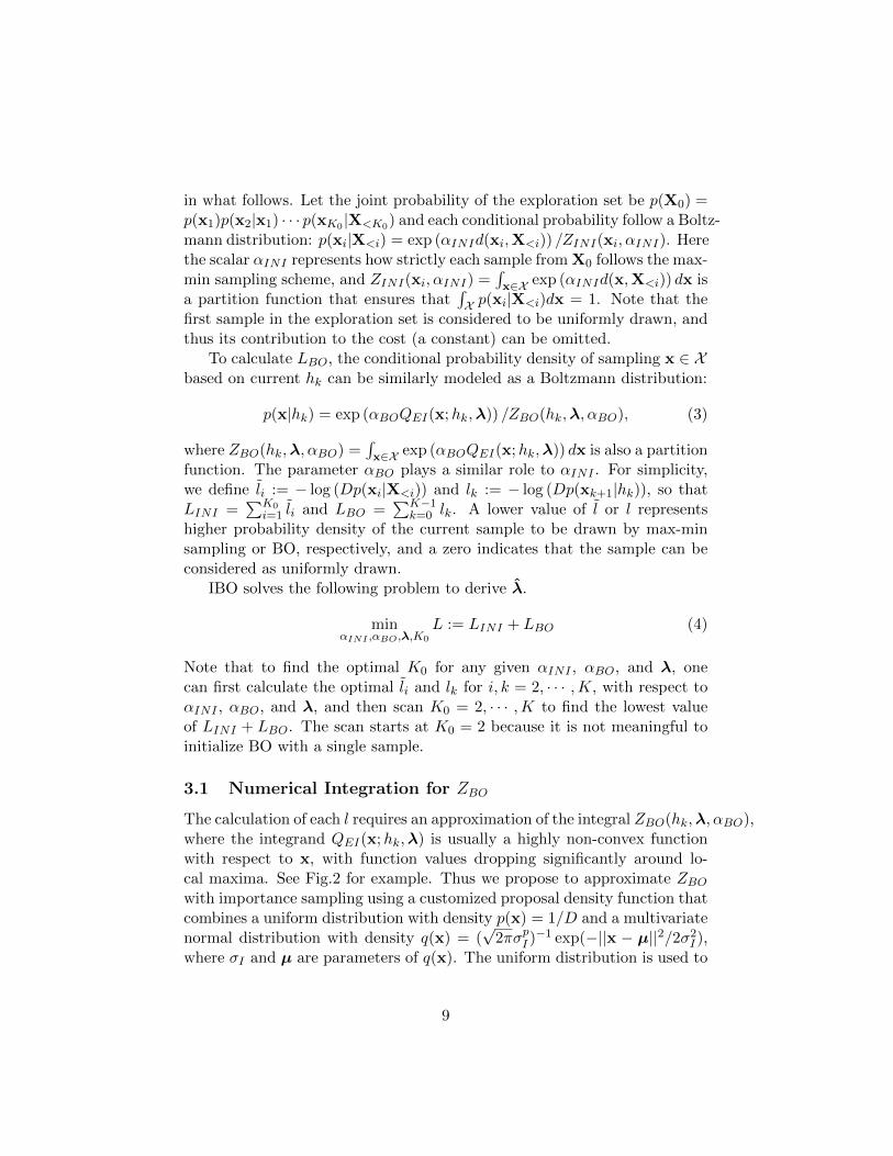
3.1 Numerical Integration for ZBO

The calculation of each l requires an approximation of the integral ZBO(hk,λ, αBO),where the integrand QEI(x;hk,λ) is usually a highly non-convex functionwith respect to x, with function values dropping significantly around lo-cal maxima. See Fig.2 for example. Thus we propose to approximate ZBOwith importance sampling using a customized proposal density function thatcombines a uniform distribution with density p(x) = 1/D and a multivariatenormal distribution with density q(x) = (

√2πσpI )

−1 exp(−||x − µ||2/2σ2I ),where σI and µ are parameters of q(x). The uniform distribution is used to

9

sample over X , while the normal distribution helps to improve the approx-imation by capturing the potential peak at the current sample xk+1. Thuswe set µ := xk+1. Let xui ∈ U for i = 1, ..., I and xnj ∈ N for j = 1, ..., J be

samples from p(x) and q(x), respectively. The approximation ZBO can becalculated by

ZBO :=∑U

DQEI(xui )

I (1 +Dq(xui ))+∑N

DQEI(xnj )

J(

1 +Dq(xnj )) , (5)

with arguments of QEI omitted for simplicity. The derivation of Eq. (5)is deferred to the appendix. Note that this approximation works underthe assumption that

∫x∈X q(x)dx ≈ 1, which is plausible as the normal

distribution is designed to have a narrow spread to match the local peak atxk+1. In this paper, the shape of this normal distribution is set by σI = 0.01universally. While the setting of σI affects the variance of the approximationof ZBO, we found this setting to perform well in practice. For ZINI , sincethe minimum Euclidean distance function in a high dimensional space withlimited samples is a relatively smooth function, we use Monte Carlo samplingfor its approximation.

3.2 Simulation studies

As a validation step, we show that IBO can recover the parameters of ageneral BO given only an observed search trajectory. If IBO can deter-mine the correct parameters (1) after a few number of iterations, (2) ina high-dimensional problem space, and (3) from a wide range of trajec-tory/parameter settings, then it could be used to recover parameters formatching a BO algorithm to an observed human search.

We use a simulation study to show that, for a given search trajectory,IBO can correctly identify the true λ provided the trajectory is sufficientlydifferent from a random search. In addition, the simulation indicates thatlearning from already-efficient search behavior (i.e., estimating λ throughIBO of an observed effective search trajectory) can lead to better BO con-vergence than the more common self-improvement methods (i.e., updatingλ by maximizing the likelihood of the observations according to the GPmodel).

3.2.1 Simulation settings and results

The simulation study is detailed as follows: We apply BO to a 30-dimensionalRosenbrock function constrained by X := [−2, 2]30. To initialize BO, we

10

use LHS to draw 10 samples from X . BO terminates when the expectedimprovement for the next iteration is less than 10−3. At each iteration,the expected improvement is maximized using a multi-start gradient de-scent algorithm [38] with 100 LHS initial guesses. A set of BO parameters,Λ = 0.01I, 0.1I, 1.0I, and 10.0I, are used to perform the search, where I isthe identity matrix. For each of the four settings, 30 independent trials arerecorded.

For each BO setting Λ, each candidate estimator Λ, and each trajectoryof length K = 5, ..., 20, we solve Eq. (4) using a grid search with GαBO :={0.01, 0.1, 1.0, 10.0} and GK0 := {2, · · · ,K}. We fix αINI to 1.0 and 10.0,and will discuss its influence to the estimation. Fig. 3 presents the resultingminimal L for all four cases and under all guesses. Each curve in eachsubplot shows how the minimal L (with respect to αBO and K0) changes asthe search continues. The means and standard deviations of L are calculatedusing the 30 trials. ZINI is approximated using a sample size of 10, 000. Inapproximating ZBO, samples from the normal and the uniform distributionsare of equal sizes (I = J = 5, 000).

3.2.2 Analysis of the results

Based on the results from this simulation, as summarized in Fig. 3, themajor finding from this simulation study is that IBO can successfully recoverthe BO parameters in cases where BO does not resemble uniform randomsampling of the design space. In the cases of Λ = 0.01I, 0.1I, 1.0I, we seethat the correct choices of Λ consistently lead to the lowest cost along thesearch process. After only one or two iterations, in nearly all cases, thecorrect parameter has the highest likelihood of all four propositions, andthis remains the case along the search. However, under large BO parameterssuch as Λ = 10.0I, the similarity between any two points in the designspace becomes close to zero, leading to (almost) uniform uncertainty andexpected improvement. Therefore this setting reduces BO to a uniformrandom sampling scheme. Fig. 3d shows that IBO does not perform wellin this situation. To better understand the behavior of IBO under near-random searches, a curious reader may find a discussion on the propertiesof the costs l and l in the Appendix.

3.2.3 Learning from others vs. self-adaptation

The above study showed that the correct BO setting λ can be learnedthrough IBO. This subsection further demonstrates the advantage of “learn-

11

Figure 3: The minimal cost L for search trajectory lengths N = 5, ..., 20with respect to GαBO and GK0 . αINI is fixed to 1.0 and 10.0. View in color.

12

ing from others” (i.e., updating λ through IBO), over “self-adaptation”(i.e., finding the MLE of λ using hk). The settings follow the above studyand results are shown in Fig. 4. First, to show the significant influenceof λ on search effectiveness, we show the convergence of two fixed searchstrategies with Λ = 0.01 and 10.0. Note that while neither converges tothe optimal solution within 50 iteration, the former is significantly moreeffective than the latter. For “self-adaptive BO”, we use a grid search(GΛ = {0.01I, 0.1I, 1.0I, 10.0I}) to find ΛGP that maximizes Eq. (1) at eachiteration, and use ΛGP to find the next sample. We show in Fig. 4b thepercentages of the four guesses being ΛGP along the search, using GΛ as theinitial guesses for BO. The “learning from others” case starts with Λ = 10.0Iand uses IBO to derive Λ from the trajectory produced by Λ = 0.01I.From Figs. 3 and 4b, we see that ΛGP does not converge to Λ = 0.01Ias quickly as IBO, which explains why “learning from others” outperforms“self-adaptation” in Fig.4a. It is worth noting that this difference in perfor-mance may be relatively dependant on the dimensionality of the problem,as the two strategies were found to have similar convergence performancewhen applied to 2D functions. One potential explanation for this is that, ina lower dimensional space, an effective ΛGP can be learned with a smallernumber of samples.

4 Case study

We now investigate how IBO may improve the performance of BO whenapplied to a vehicle design and control problem.

4.1 Dimension reduction for player’s control signals

The solution data from each game play consists of (1) the final gear ratio,(2) the recorded acceleration and braking signals, and (3) the correspond-ing game score. The length of a raw control signal matches that of thetrack, which has 18160 distance steps. Encoding control signals to a low di-mensional space is feasible since common acceleration and braking patternsexist across all plays. In [11], this was done by introducing manually definedstate-dependent basis functions (i.e., polynomials of the velocity of the car,slope of the track, distance to the terminal, remaining battery energy, andtime spent) to parameterize the control signals. The underlying assumptionthat human players are aware of all the state-dependent bases is untested.

In this paper, we perform dimension reduction based on evidence thathuman beings often solve high dimensional problem by performing problem

13

Figure 4: (a) Comparison on BO convergence using four algorithmic settings:(orange) Λ = 10.0I, (green) Λ = 0.01I, (grey) the MLE of Λ is used foreach new sample, and (red) the initial setting Λ = 10.0I is updated byIBO using the trajectory from Λ = 0.01I. (b) The percentages of estimatedΛMLE along the number of iterations, averaged over the cases with Λ ={0.01I, 0.1I, 1.0I, 10.0I} and 30 trials for each case. View in color.

14

abstraction and using a hierarchical search [39–43]. In the context of the ec-oRacer game, we hypothesize that players segment the track into m discretesections, and make separate control decisions in each segment. Mathemat-ically, this is equivalent to projecting observed signals onto m independentbasis, which can be elegantly addressed by ICA [44]. Compared with Prin-cipal Component Analysis, where the bases minimize the covariance of thedata, our ICA implementation maximizes the Kullback-Leibler divergencebetween all bases pairs, and is more suitable for non-Gaussian signals, suchas the control data from this game (i.e., the acceleration/braking signalsacross players at each step along the track are unlikely to follow a Gaussiandistribution).

Much like PCA, the choice of the number of ICA bases requires a balancebetween fidelity and practicality. While it is theoretically possible to find the“most likely” number of bases using information-theoretic criteria for modelselection [45]3, we chose to use 30 bases because (1) over 95% of the varianceis explained, and (2) the resultant solution space (30 control variables andone design variable) is small enough for BO to be effective.

4.2 Derivation of λ and λGP

We apply IBO to two players, referred to as “P2” and “P3”, who achievedthe second and third highest score within 31 and 73 plays, respectively,much less than the 150 plays from the achiever of the highest score. Todo so, we first encode all control solutions from the two players using thelearned ICA bases. Together with the final drive ratios, all solutions arethen normalized to be within [−1, 1]31. IBO is performed separately on P2and P3. We found that the probability for either player to have followedthe max-min sampling scheme is lower than that of following BO, as theminimal values of l(xk, αINI) for k = 2, ..., 31 (with respect to αINI) aredominated by those of l(xk, αBO). This means that the players were notlikely to have performed an exploration before they started trying to improvetheir performance. This finding is reasonable, as the scoring mechanism inecoRacer game, just like in other racer games with fairly predictable vehicle

3For completeness, we used 1000 PCA components as preprocessing to obtain the mostlikely number of ICA components under three suitable criteria: Minimum DescriptionLength, Akaike Information Criterion, and Kullback Information Criterion, as 187, 464,and 373, respectively, using the method from [45]. While these dimensionalities could makesense from a neurological perspective (e.g., given that the game takes 36 seconds, a decisioninterval of 36s/187 = 192ms is close to the range for the time-frame of attentional blink,which is 200-500 ms [46]), the resultant high-dimensional solution spaces are unfavorablefor BO.

15

Figure 5: ICA bases learned from all human plays and the ecoRacer track.Vertical lines on the track correspond to the peak locations of the bases.

16

dynamics, can be understood by the player early on. Therefore, the searchfor λ is performed by solving Eq. (4) with λ ∈ [0.01, 10.0]31, αBO ∈ GαBO ,and a minimal number of initial samples (K0 = 2) required for BO. Forcomparison purpose, we obtain λGP using plays from P2, which representsa case where BO parameters are fine-tuned by the observed game plays,without trying to explain why these solutions were searched by the player.

Due to the non-convexity of Eq. (4) and Eq. (1), gradient-based searchesusing a series of 10 initial guesses are conducted to avoid inferior local so-lutions. Finite difference is used for gradient approximation. Both λ andλGP are calculated offline, and fixed during the execution of BO.

4.3 Comparison of BO performance

Fig. 6 compares the BO performance under λ (for P2 and P3), λGP andΛ = I. In each case, we start with the first two plays from the players, andrun 180 BO iterations. Similar to the simulation study, results are reportedusing 20 trials due to the stochastic nature of BO. Due to the small trialnumber, bootstrap variance estimators are reported as the shades around theaverage in the figure. λ outperforms the other two settings consistently alongthe search with statistical significance. The BO performance by mimickingP2 is slightly better than that of P3.

The result shows that BO can be improved noticeably by learning fromP2 and P3. However, the players’ search are not fully mimicked by IBO, asthey improved much faster than the modified BO does, indicating that theproposed model still has room for improvement. Nevertheless, the IBO im-plementation still achieves the closest performance to the players’ among allBO instances, and it is the only algorithm that achieved better performancethan the players’ best play within 100 iterations. This result demonstratesthe potential of IBO to continue an effective human search after the playerquits, with an improved search performance from a standard BO.

For completeness, we also note that in all cases, the BO identifies the trueoptimal final drive ratio at the end of the search. We also qualitatively com-pare the best human solution with one BO solution with high score, alongwith the theoretically optimal solution in Fig. 7. The result indicates thatwhile these control strategies yield similar scores, they are quantitatively dif-ferent, although braking towards the end is observed as a common strategy.Human search data are documented at ecoracer.herokuapp.com/results,where the best players’ solution strategies are published.

17

Figure 6: The residual of current best score vs. the known best score, withsettings λ (IBO, red), λGP (MLE, blue), and the default λ = I (green).Results are shown as averages over 30 trials. One-sigma confidence intervalsare calculated via 5000 bootstrap samples. Red and black dots are scoresfrom P2 and P3, respectively.

Figure 7: Qualitative comparison on control strategies from the theoreticaloptimal solution (top), one of the BO solutions (middle), and the best playersolution (bottom).

18

5 Discussion

The above study provided a starting point for learning optimization algo-rithms based on human solution-search data. Yet, many pressing questionsremain unanswered. This section will address a few notable ones. Somepotential answers to these questions will rely on readers’ familiarity withInverse Reinforcement Learning [19, 47, 48] (IRL, also called apprenticeshiplearning [49, 50] and inverse optimal control [51]). To familiarize readerswith this topic, a discussion on the connection between IBO and IRL isprovided in Subsec. 5.2.

5.1 Limitations and potential values of IBO

From the case study, a strategy learning through IBO outperformed defaultalgorithms, but is yet to reach the performance of the best human solver.This indicates potential room to further improve the algorithm. In thefollowing, we discuss notable limitations of IBO. We shall also note thatthese also apply to the general problem of designing optimization algorithmsthrough human demonstrations (called DO in what follows).

Model of human search strategies: Studies in cognitive science haveput forth several core ingredients of human intelligence, including intuitivephysics [52–55], problem decomposition skills [42,56,57], ability in learning-to-learn [58], and others [10]. While evidence has shown the connection be-tween BO and human search [18], suitable models for human search strate-gies can be problem dependent. For example, for low-dimensional designproblems, Egan et al. [59] showed that people adopting univariate searchare more likely to achieve effective search. This result is supported by ear-lier psychological studies on how children perform scientific reasoning, andthus may be useful to explain how people identify unfamiliar systems. How-ever, univariate search may not reflect how people search for solutions ina familiar context (such as car driving) and with a large number of con-trol and design variables to tune, as is the situation of the ecoRacer game.For such high-dimensional and physics-based design and control problems, apotentially reasonable human search model could be to incorporate humanintuitive physics models into the evaluation of the expected improvement.Thus instead of estimating GP parameters, one could estimate a statisticalmodel of the state-space equations of the dynamical system, which influ-ences the expected improvement. At a more abstract level, the fundamentalchallenge in understanding how a human search strategy should be modeledis the lack of knowledge about the functional form of the local objective

19

(i.e., the Q-function) that governs the generation of new solutions duringthe search based on the current state (cumulative knowledge learned by thehuman solver). As we will discuss later in this section, this challenge is alsoa key topic in IRL. Not surprisingly, one notable solution from IRL to thisproblem is in fact to use non-parametric models such as GP [19,60].

Uncertainty in estimation: A limited amount of demonstrationscould be insufficient to provide a good estimation of the BO parameters,even though the underlying parameters are the effective ones. One potentialsolution to this could be to create a reward mechanism in the crowdsourcingsetting, where the reward is determined by both the observed search effec-tiveness of each human solver, and the uncertainty in the estimation of theirsearch strategy. In the context of BO, this uncertainty can be measuredby the covariance of the estimator, i.e., the Hessian of the cost function inEq. (4). For people with effective search yet high estimation uncertainty,we can solicit more solutions from them by offering rewards. It would alsobe interesting to understand the influence of the properties of the problem,e.g., the size of the solution space, on the convergence of the estimation.

Knowledge transferability: The third limitation concerns the trans-ferability of knowledge (search strategies) learned from one task (an opti-mization problem) to others. This limitation also leads to the question ofhow “effectiveness” of searches shall be measured, as we are not yet able totell in what condition a strategy that has high rate of improvement (such asP2 in ecoRacer) will continue to produce better solutions than other strate-gies in a long term. The same issue, however, exists in IRL: e.g., a controlpolicy learned for pancake flipping does not guarantee optimal egg flippingdue to the differences in physical properties between pancakes and eggs.One solution to this in IRL is to allow the policy to adjust to new prob-lem settings, by correcting the state transition model according to the newobservations. This solution may also be applied to IBO. In the context ofecoRacer, knowledge such as “starting acceleration at the beginning of thetrack” could be considered as a universal strategy and requires less explo-ration, while the actual duration for executing this strategy may differ acrossproblem settings. Therefore, it could be more effective for BO to adjust itsparameters based on the ones that are learned from human demonstrationson a similar problem, rather than learning from scratch.

To summarize, IBO could be a valuable tool for machines to mimichuman search behavior when (1) the underlying human search mechanismfollows BO; (2) the demonstration is sufficient for estimating the true BOparameters with low variances, and (3) the true optimal BO parameters fora long-term search can be estimated based on an effective short-term search.

20

5.2 The difference between learning to search and learninga solution

The proposed IBO approach can be considered as a way to design opti-mization algorithms with human guidance, and is mathematically similar toIRL. In order to explain the similarities and differences between the two, wefirst introduce Markov Decision Process (MDP) and Reinforcement Learning(RL), and make an analogy between MDP and an optimization algorithm.

5.2.1 Preliminaries on MDP and RL

A MDP is defined by a tuple < S,A, T ,R, γ, b0 > where: S is a set of states;A is a set of actions; the state transition function T (s,a, s′) determines theprobability of changing from state s to s′ when action a is taken; R(s,a)is the instantaneous reward of taking action a at state s; γ ∈ [0, 1) is thediscount factor of future reward; b0(s) specifies the probability of startingthe process at state s. In RL, a control policy π is a mapping from a stateto an action, i.e., π : S → A. The long-term value of π for a starting states can be calculated by V π(s) = R(s, π(s)) + γ

∑s′∈S T (s, π(s), s′)V π(s′),

and thus the value of π over all possible starting states is the expectationV π =

∑s∈S b0(s)V π(s). A common way to represent a control policy is to

introduce a Q-function Q(s,a;λ) with unknown control parameters λ, andlet the policy be a(s) = argmaxAQ(s,a;λ). RL identifies the optimal λ thatmaximizes V π.

5.2.2 MDP vs. optimization algorithm

An optimization algorithm defines a decision process: Its instantaneous re-ward is the improvement in the objective value achieved by each new sample,and the cumulative reward represents the total improvement in the objectivewithin a finite number of iterations; its state contains the current solution(in X ), the corresponding objective value, and potentially the gradient andhigher-order derivatives of the objective function at the current solution;its action is the next solution to evaluate; and its state transition is gov-erned by the optimization algorithm and its parameters. This is similarto MDP where the state transition is affected by the control parameters.The decision process defined by an optimization algorithm, however, is usu-ally non-Markovian, as the new solutions rely on the entire search trajectory.Note that it is still possible to consider the optimization process as an MDP,by redefining the state as the continuously growing search trajectory, i.e.,

21

elements in the state set S shall represent all possible search trajectories,rather than samples in X .

5.2.3 IRL vs. IBO

RL algorithms identify an optimal control policy for an MDP with a givenreward function. However, real-world applications hardly have explicit def-initions of rewards, e.g., the reward for “driving a car” cannot be explicitlydefined, although people form control policies based on their inherent re-ward (preference). Therefore, control policy for such applications can belearned more effectively through demonstrations of human beings, whichare assumed to be optimal according to the inherent reward of the demon-strator. IRL techniques have thus been developed to identify the reward(and consequently the Q-function and the optimal control policy) that ex-plains human demonstrations, either by estimating the reward parametersso that the demonstrated policy has a higher value than any other policiesby a margin [47, 49, 61, 62], or by finding the maximum likelihood controlparameters directly [48,63].

The IBO approach introduced in this paper is closely related to lattertype of IRLs, and more precisely, to the maximum entropy method of Ziebartet al. [48]. Briefly, the maximum entropy IRL proposes the following MLEof parameters λ based on a set of demonstrations h:

λ = argmaxλ logP (h|λ)

= argmaxλ logexp

(∑(si,ai)∈hR(si,ai,λ)

)∏

(si,ai)∈h Zi(λ),

(6)

where Zi(λ) is a partition function for the visited state si. One can no-tice the similarities between Eq. (6) and Eq. (4): (1) Both are maximumlikelihood parameter estimations related to an instantaneous cost, i.e., thereward in Eq. (6) and the expected improvement in IBO. (2) Both involvespartition functions that are computationally expensive, and dependent onthe parameters λ. Due to this dependency, a direct Markov-Chain MonteCarlo (MCMC) sampling in the space of λ (e.g., as in [63]) cannot be ap-plied to optimize the likelihood function since the partition values for twodifferent samples of λ do not cancel. Ziebart et al. discussed on alternativeapproach to address this computational challenge, by using the “ExpectedEdge Frequency Calculation” algorithm that has a complexity of O(N |S||A|)for each gradient calculation of the objective in Eq. (6), where N is a large

22

number [48]. However, this approach can be infeasible for the IBO estima-tion problem in Eq. (4) since (1) the space X is usually continuous, and (2)even with a discretization of X , the enormous size of S and A can easilymake the calculation intractable, based on the discussion in Sec. 5.2.2.

Further, one shall notice that IRL and IBO uses different assumptionsabout human demonstrations: Demonstrations in IRL are assumed to benear-optimal. Thus learning from them leads to an optimal control policyfor an MDP. Demonstrations in IBO, on the other hand, are assumed to befrom an effect search strategy, yet are not necessarily optimal. Thus learningfrom them leads to an optimization algorithm, rather than a solution. Thisdifference affects the application of the two: IRL can be used when themachine is told to mimic existing solutions, by understanding why thesesolutions are considered good, e.g., it answers the question “why do peopleflip pancakes this way?”; IBO can be used when the machine is meant tomimic the process of searching for good solutions, by understanding how toevaluate the expected improvement of solutions, e.g., it answers the question“how did people figure out this way of pancake flipping?”.

6 Conclusions

In this paper, we attempted to address a dilemma in design crowdsourcing:While human beings acquire more advanced intelligence than machines insolving certain types of optimal design problems, soliciting valuable solutionsthrough existing crowdsourcing mechanisms is not cost-effective due to thelack of control over crowd participation and the problem-specific qualifica-tion of the crowd. Based on the previous finding that more people acquiregood searching strategies than good solutions, we proposed in this paper tomimic human search demonstrations by inversely learn a Bayesian optimiza-tion algorithm, so that long-term search can be executed more effectivelyby the computer even when human solvers abandon the problem. Throughsimulation and case studies, we showed improved performance of BO whenit is equipped with parameters learned through an effective human search.However, the significant performance gap between a human demonstratorand the proposed algorithm in the case study suggested room for improve-ment of the algorithm. Future investigation will focus on closing this gapby exploring more suitable cognitive models of human solution searching forspecific types of optimal design problems.

23

Acknowledgement

This work has been supported by the National Science Foundation underGrant No. CMMI-1266184. This support is gratefully acknowledged.

References

[1] Cooper, S., Khatib, F., Treuille, A., Barbero, J., Lee, J., Beenen, M.,Leaver-Fay, A., Baker, D., Popovic, Z., et al., 2010. Foldit. http:

//fold.it.

[2] Khatib, F., Cooper, S., Tyka, M. D., Xu, K., Makedon, I., Popovic,Z., Baker, D., and Players, F., 2011. “Algorithm discovery by proteinfolding game players”. Proceedings of the National Academy of Sciences,108(47), pp. 18949–18953.

[3] Lee, J., Kladwang, W., Lee, M., Cantu, D., Azizyan, M., Kim, H.,Limpaecher, A., Yoon, S., Treuille, A., and Das, R., 2014. eterna.http://eterna.cmu.edu.

[4] Lee, J., Kladwang, W., Lee, M., Cantu, D., Azizyan, M., Kim, H.,Limpaecher, A., Yoon, S., Treuille, A., and Das, R., 2014. “Rna designrules from a massive open laboratory”. Proceedings of the NationalAcademy of Sciences, 111(6), pp. 2122–2127.

[5] Kawrykow, A., Roumanis, G., Kam, A., Kwak, D., Leung, C., Wu, C.,Zarour, E., Sarmenta, L., Blanchette, M., Waldispuhl, J., et al., 2012.“Phylo: a citizen science approach for improving multiple sequencealignment”. PloS one, 7(3), p. e31362.

[6] Sung, J., Jin, S. H., and Saxena, A., 2015. “Robobarista: Object partbased transfer of manipulation trajectories from crowd-sourcing in 3dpointclouds”. arXiv preprint arXiv:1504.03071.

[7] Le Bras, R., Bernstein, R., Gomes, C. P., Selman, B., and Van Dover,R. B., 2013. “Crowdsourcing backdoor identification for combinatorialoptimization”. In Proceedings of the Twenty-Third international jointconference on Artificial Intelligence, AAAI Press, pp. 2840–2847.

[8] Ren, Y., Bayrak, A. E., and Papalambros, P. Y., 2016. “ecoracer:Game-based optimal electric vehicle design and driver control usinghuman players”. Journal of Mechanical Design, 138(6), p. 061407.

24

[9] Schrope, M., 2013. “Solving tough problems with games”. Proceedingsof the National Academy of Sciences, 110(18), pp. 7104–7106.

[10] Lake, B. M., Ullman, T. D., Tenenbaum, J. B., and Gershman, S. J.,2016. “Building machines that learn and think like people”. arXivpreprint arXiv:1604.00289.

[11] Ren, Y., Bayrak, A. E., and Papalambros, P. Y., 2015. “ecoracer:Game-based optimal electric vehicle design and driver control usinghuman players”. In ASME 2015 International Design Engineering Tech-nical Conferences and Computers and Information in Engineering Con-ference, American Society of Mechanical Engineers, pp. V02AT03A009–V02AT03A009.

[12] Jones, D., Schonlau, M., and Welch, W., 1998. “Efficient global op-timization of expensive black-box functions”. Journal of Global Opti-mization, 13(4), pp. 455–492.

[13] Brochu, E., Cora, V. M., and De Freitas, N., 2010. “A tutorial onbayesian optimization of expensive cost functions, with application toactive user modeling and hierarchical reinforcement learning”. arXivpreprint arXiv:1012.2599.

[14] Rasmussen, C. E., 2006. “Gaussian processes for machine learning”.MIT Press.

[15] Lucas, C. G., Griffiths, T. L., Williams, J. J., and Kalish, M. L., 2015.“A rational model of function learning”. Psychonomic bulletin & review,22(5), pp. 1193–1215.

[16] Wilson, A. G., Dann, C., Lucas, C., and Xing, E. P., 2015. “Thehuman kernel”. In Advances in Neural Information Processing Systems,pp. 2854–2862.

[17] Rasmussen, C. E., and Ghahramani, Z., 2001. “Occam’s razor”. Ad-vances in neural information processing systems, pp. 294–300.

[18] Borji, A., and Itti, L., 2013. “Bayesian optimization explains humanactive search”. In Advances in neural information processing systems,pp. 55–63.

[19] Levine, S., Popovic, Z., and Koltun, V., 2011. “Nonlinear inverse re-inforcement learning with gaussian processes”. In Advances in NeuralInformation Processing Systems, pp. 19–27.

25

[20] Deisenroth, M. P., Neumann, G., Peters, J., et al., 2013. “A surveyon policy search for robotics.”. Foundations and Trends in Robotics,2(1-2), pp. 1–142.

[21] Calandra, R., Gopalan, N., Seyfarth, A., Peters, J., and Deisenroth,M. P., 2014. “Bayesian gait optimization for bipedal locomotion”.In International Conference on Learning and Intelligent Optimization,Springer, pp. 274–290.

[22] Cully, A., Clune, J., Tarapore, D., and Mouret, J.-B., 2015. “Robotsthat can adapt like animals”. Nature, 521(7553), pp. 503–507.

[23] Pretz, J. E., 2008. “Intuition versus analysis: Strategy and experiencein complex everyday problem solving”. Memory & cognition, 36(3),pp. 554–566.

[24] Linsey, J. S., Tseng, I., Fu, K., Cagan, J., Wood, K. L., and Schunn,C., 2010. “A study of design fixation, its mitigation and perception inengineering design faculty”. Journal of Mechanical Design, 132(4),p. 041003.

[25] Daly, S. R., Yilmaz, S., Christian, J. L., Seifert, C. M., and Gonzalez,R., 2012. “Design heuristics in engineering concept generation”. Journalof Engineering Education, 101(4), p. 601.

[26] Cagan, J., Dinar, M., Shah, J. J., Leifer, L., Linsey, J., Smith, S.,and Vargas-Hernandez, N., 2013. “Empirical studies of design think-ing: past, present, future”. In ASME 2013 International Design En-gineering Technical Conferences and Computers and Information inEngineering Conference, American Society of Mechanical Engineers,pp. V005T06A020–V005T06A020.

[27] Bjorklund, T. A., 2013. “Initial mental representations of design prob-lems: Differences between experts and novices”. Design Studies, 34(2),pp. 135–160.

[28] Egan, P., and Cagan, J., 2016. “Human and computational ap-proaches for design problem-solving”. In Experimental Design Research.Springer, pp. 187–205.

[29] Cagan, J., and Kotovsky, K., 1997. “Simulated annealing and the gen-eration of the objective function: a model of learning during problemsolving”. Computational Intelligence, 13(4), pp. 534–581.

26

[30] Landry, L. H., and Cagan, J., 2011. “Protocol-based multi-agent sys-tems: examining the effect of diversity, dynamism, and cooperationin heuristic optimization approaches”. Journal of Mechanical Design,133(2), p. 021001.

[31] McComb, C., Cagan, J., and Kotovsky, K., 2016. “Drawing inspira-tion from human design teams for better search and optimization: Theheterogeneous simulated annealing teams algorithm”. Journal of Me-chanical Design, 138(4), p. 044501.

[32] Thrun, S., and Pratt, L., 1998. “Learning to learn: Introduction andoverview”. In Learning to learn. Springer, pp. 3–17.

[33] Wang, J. X., Kurth-Nelson, Z., Tirumala, D., Soyer, H., Leibo, J. Z.,Munos, R., Blundell, C., Kumaran, D., and Botvinick, M., 2016.“Learning to reinforcement learn”. arXiv preprint arXiv:1611.05763.

[34] Andrychowicz, M., Denil, M., Gomez, S., Hoffman, M. W., Pfau, D.,Schaul, T., and de Freitas, N., 2016. “Learning to learn by gradientdescent by gradient descent”. In Advances in Neural Information Pro-cessing Systems, pp. 3981–3989.

[35] Hansen, N., Muller, S. D., and Koumoutsakos, P., 2003. “Reducing thetime complexity of the derandomized evolution strategy with covariancematrix adaptation (cma-es)”. Evolutionary computation, 11(1), pp. 1–18.

[36] Jones, D. R., Perttunen, C. D., and Stuckman, B. E., 1993. “Lips-chitzian optimization without the lipschitz constant”. Journal of Opti-mization Theory and Applications, 79(1), pp. 157–181.

[37] Sahinidis, N. V., 1996. “Baron: A general purpose global optimizationsoftware package”. Journal of global optimization, 8(2), pp. 201–205.

[38] Zhu, C., Byrd, R. H., Lu, P., and Nocedal, J., 1994. “L-bfgs-b: Fortransubroutines for large scale bound constrained optimization”. ReportNAM-11, EECS Department, Northwestern University.

[39] McGovern, A., Sutton, R. S., and Fagg, A. H., 1997. “Roles of macro-actions in accelerating reinforcement learning”. In Grace Hopper cele-bration of women in computing, Vol. 1317.

27

[40] McGovern, A., and Barto, A. G., 2001. “Automatic discovery of sub-goals in reinforcement learning using diverse density”. Computer Sci-ence Department Faculty Publication Series, p. 8.

[41] Dietterich, T. G., 1998. “The maxq method for hierarchical reinforce-ment learning.”. In ICML, Citeseer, pp. 118–126.

[42] Kulkarni, T. D., Narasimhan, K. R., Saeedi, A., and Tenenbaum, J. B.,2016. “Hierarchical deep reinforcement learning: Integrating temporalabstraction and intrinsic motivation”. arXiv preprint arXiv:1604.06057.

[43] Botvinick, M., and Weinstein, A., 2014. “Model-based hierarchicalreinforcement learning and human action control”. Phil. Trans. R.Soc. B, 369(1655), p. 20130480.

[44] Stone, J. V., 2004. Independent component analysis. Wiley OnlineLibrary.

[45] Hui, M., Li, J., Wen, X., Yao, L., and Long, Z., 2011. “An empiricalcomparison of information-theoretic criteria in estimating the numberof independent components of fmri data”. PloS one, 6(12), p. e29274.

[46] Tombu, M. N., Asplund, C. L., Dux, P. E., Godwin, D., Martin, J. W.,and Marois, R., 2011. “A unified attentional bottleneck in the humanbrain”. Proceedings of the National Academy of Sciences, 108(33),pp. 13426–13431.

[47] Ng, A. Y., Russell, S. J., et al., 2000. “Algorithms for inverse reinforce-ment learning.”. In Icml, pp. 663–670.

[48] Ziebart, B. D., Maas, A. L., Bagnell, J. A., and Dey, A. K., 2008. “Maxi-mum entropy inverse reinforcement learning.”. In AAAI, pp. 1433–1438.

[49] Abbeel, P., and Ng, A. Y., 2004. “Apprenticeship learning via inversereinforcement learning”. In Proceedings of the twenty-first internationalconference on Machine learning, ACM, p. 1.

[50] Abbeel, P., Coates, A., and Ng, A. Y., 2010. “Autonomous helicopteraerobatics through apprenticeship learning”. The International Journalof Robotics Research.

[51] Dvijotham, K., and Todorov, E., 2010. “Inverse optimal control withlinearly-solvable mdps”. In Proceedings of the 27th International Con-ference on Machine Learning (ICML-10), pp. 335–342.

28

[52] Spelke, E. S., Gutheil, G., and Van de Walle, G., 1995. “The develop-ment of object perception.”.

[53] Baillargeon, R., Li, J., Ng, W., and Yuan, S., 2009. “An account ofinfants’ physical reasoning”. Learning and the infant mind, pp. 66–116.

[54] Bates, C. J., Yildirim, I., Tenenbaum, J. B., and Battaglia, P. W.,2015. “Humans predict liquid dynamics using probabilistic simulation”.In Proceedings of the 37th annual conference of the cognitive sciencesociety.

[55] Gershman, S. J., Horvitz, E. J., and Tenenbaum, J. B., 2015. “Compu-tational rationality: A converging paradigm for intelligence in brains,minds, and machines”. Science, 349(6245), pp. 273–278.

[56] Fodor, J. A., 1975. The language of thought, Vol. 5. Harvard UniversityPress.

[57] Biederman, I., 1987. “Recognition-by-components: a theory of humanimage understanding.”. Psychological review, 94(2), p. 115.

[58] Harlow, H. F., 1949. “The formation of learning sets.”. Psychologicalreview, 56(1), p. 51.

[59] Egan, P., Cagan, J., Schunn, C., and LeDuc, P., 2015. “Synergistichuman-agent methods for deriving effective search strategies: the caseof nanoscale design”. Research in Engineering Design, 26(2), pp. 145–169.

[60] Choi, J., and Kim, K.-E., 2012. “Nonparametric bayesian inverse re-inforcement learning for multiple reward functions”. In Advances inNeural Information Processing Systems, pp. 305–313.

[61] Ratliff, N. D., Bagnell, J. A., and Zinkevich, M. A., 2006. “Maximummargin planning”. In Proceedings of the 23rd international conferenceon Machine learning, ACM, pp. 729–736.

[62] Syed, U., and Schapire, R. E., 2007. “A game-theoretic approach toapprenticeship learning”. In Advances in neural information processingsystems, pp. 1449–1456.

[63] Ramachandran, D., and Amir, E., 2007. “Bayesian inverse reinforce-ment learning”. Urbana, 51, p. 61801.

29

Appendix

Derivation of Eq. (5)

Let p(x) = 1/D and q(x) be a uniform and a normal density function,respectively, D be the size of X , and f(x) be the function to be integrated.Also let I and J be the sample sets drawn from these two distributions,with sizes I := |I| and J := |J |. We have∫

f(x)dx = D

∫f(x)p(x)dx

= D

(∫f(x)p(x)2

p(x) + q(x)dx+

∫f(x)q(x)p(x)

p(x) + q(x)dx

)≈ D

(1

I

∑I

f(x)p(x)

p(x) + q(x)+

1

J

∑J

f(x)p(x)

p(x) + q(x)

)

=∑I

f(x)D

I(1 +Dq(x))+∑J

f(x)D

J(1 +Dq(x))

IBO behavior under near-random search

Properties of l and l From Sec. 3.1, the unbiased estimation of l(x, αBO)through importance sampling is:

l(x, αBO) = − logexp(αBOQEI(x))

ZBO/D. (7)

l(x, αBO) has the following properties. Property 1: αBO = 0 leads tol(x, 0) = 0, indicating that x is uniformly sampled. One can see that the op-timal cost of LBO is non-positive, as one can always achieve LBO = 0 by con-sidering samples to be uniformly drawn. Property 2: When the expectedimprovement function is constant almost everywhere, i.e., Pr(QEI(x) =C) = 1, we have Pr(l(x, αBO) = 0) = 1. This is because a uniformlydrawn initial guess will almost surely satisfy the optimality condition formaximizing a constant function. Property 3: Notice that 1 + Dq(xi) ≈ 1

for xi ∈ U due to the small σI (see Sec. 3.1), and exp(αBOQEI(xi))1+Dq(xi)

≈ 0 for

large D and small αBO. The partial derivative of l(x, 0) with respect to αBOcan be approximated as:

∂l(x, 0)

∂αBO= c(αBO)

∑U

∆ai, (8)

30

where c(αBO) > 0 and ∆ai := QEI(xi)−QEI(x). Here we need to introducea conjecture: Let QEI :=

∫X QEI(x)dx/D be the average expected improve-

ment, and A :=∫X 1(QEI(x) > QEI)dx be the measure of a subspace where

the sampled expected improvement value is higher than QEI . A decreasesfrom above to below D/2 along the increase of the BO sample size. In otherwords, a uniformly drawn sample has more than 50% of chance to have anexpected improvement value higher than QEI at the early stage of BO, andless than 50% at the late stage.

One evidence of the conjecture is illustrated in Fig. 2: In the first itera-tion, QEI is slightly lower than 0.5 while the majority of X has QEI > QEI ;in the fourth iteration, however, only a small region around the peak hasQEI > QEI . Using this conjecture, we can show that

∑U ∆ai < 0 when the

sample size is small, thus ∂l(x,0)∂αBO

< 0. Together with Property 1, we have

l(x, αBO) < 0 for a small αBO and a small sample size.Property 4: We notice that in this experiment, the discrepancy be-

tween LHS and the modeled max-min sampling scheme leads to overall high(positive) l values, indicating that the samples are not likely follow thisscheme. This is consistent with the fact that LHS is not exactly the sameas max-min sampling, at least until all of h0 has been considered. We alsosee that negative l values can be observed when αINI is low, suggesting thatthe LHS samples can be better explained by a loosely executed max-minsampling scheme than a strict one.

Discussion on findings from Fig. 3 We now summarize a complete listof findings based on these properties. Finding 1: A comparison betweenαINI = 1.0 and 10.0 leads to a finding consistent with Property 4. Sincethe samples are not likely to be drawn from a strictly executed max-minsampling scheme, the entire search trajectory is considered to be createdfrom BO in the case of αINI = 10.0. While the early samples (less than 10)can be considered as from max-min sampling when αINI = 1.0 (l < 0), thelow magnitude of l causes this difference to be only visible in the case ofΛ = 10.0I, where the magnitude of l is also low. Finding 2: IBO correctlyidentifies the true Λ within a few iterations after the initial exploration,except for the case of Λ = 10.0I. To explain this exception, we first notethat Λ = 10.0I leads to an expected improvement function that is constantalmost everywhere (except for the sampled locations where QEI = 0) andthus BO reduces to uniform sampling. From Property 2, LBO = 0 almostsurely when we have the correct guess on Λ. Also recall from Property 4that LINI > 0 when αINI is high. The above two together explain why with

31

the correct guess of Λ = 10.0I, we have L close to zero when αINI = 10.0and slightly negative when αINI = 1.0.4

To explain the negative L values for the incorrect guesses of Λ, we useProperty 3 to show that when the sample size is small and the expectedimprovement function is not flat, LBO < 0 for a small αBO, and thus L < 0.To summarize, Finding 2 suggests that for a search trajectory with a lim-ited length that resembles a random search, the proposed IBO approach willconsider it being derived from a BO that loosely solves Eq. 4. However, thiscaveat is of little practical concern, since (1) a random search rarely outper-forms BO with non-trivial settings, and (2) a BO with low αBO (instead ofhigh Λ) can equally simulate a random search.

4But why does the guess of Λ = 10.0I lead to significantly decreasing L in the otherthree cases? This is because in those cases, BO does not resemble random sampling, i.e.,the sequences of samples are more clustered. When a new sample is among this cluster, itssimilarities to existing ones are non-zero even when a large Λ is assumed, due to the smallEuclidean distance among the pairs. And in turn, the expected improvement function haspeaks within the clusters, and remains constant far away from them, rather than being aconstant almost everywhere. As a result, the optimal value of l(x, αBO) with respect toαBO becomes negative, even when Λ is incorrectly guessed as 10.0I.

32