Learning-by-Doing in the Newsvendor Problem

A Laboratory Investigation of the Role of Experience and Feedback

Gary E Bolton & Elena Katok†

Smeal College of Business

Penn State University

September 15, 2004

We investigate learning-by-doing in the newsvendor inventory problem. An earlier study

observed that decision makers tend to anchor orders away from the expected profit

maximizing order. We study enhancements to the learning environment suggested by the

behavioral literature. Extended experience improves performance some but feedback

enhancements do little. A manipulation with a strong positive effect constrains inventory

policy to a standing order for multiple periods, precluding responses to short term

fluctuations in demand. With experience, our newsvendors collectively achieve over

90% of expected profit potential. It turns out that this kind of hands-on learning is more

effective than providing newsvendors with an upfront statistical analysis that includes the

expected profitability of orders. The results speak to the kinds of training and decision

support that might improve the performance of inventory decision makers.

Keywords: Newsvendor problem, feedback, behavioral operations management, supply

chain management, experimental economics.

† University Park, PA 16802. Bolton: 814-865-0611, gbolton@psu.edu; Katok: 814-863-2180, ekatok@psu.edu.

1. INTRODUCTION

This paper presents a laboratory investigation of learning-by-doing in the newsvendor

problem, a foundational paradigm for the study of inventory in the face of stochastic demand.1

While the solution to the newsvendor problem is well known to operations researchers, many

people make suboptimal choices even with repeated exposure (Schweitzer and Cachon 2000).

People are proficient at solving related stochastic choice problems, and this suggests that

modifications to the learning environment might help them here.2 The specific question we

address is: What enhancements to experience or feedback lead to better inventory decisions?

The answer speaks to both descriptive and prescriptive issues: To the conditions under which the

rational optimizing assumption is a satisfactory approximation of behavior, and to the training or

decision support that would benefit inventory decision makers. On the latter score, analytical

techniques and experienced judgment would ideally work in tandem; understanding learning-by-

doing is a step towards prescribing the most utilitarian analytical tools.3

Virtually all stochastic inventory theory relies in one way or another on the newsvendor

problem (Porteous 1990). Understanding inventory ordering behavior is critical to designing

effective supply chain incentive systems (ex., Cachon 2002). A common assumption behind the

prescriptions that flow from these various models is that the newsvendor will act optimally to

maximize expected profit. But the conditions under which one can expect or induce optimal

ordering are presently a missing link in the literature.

Understanding behavior in the standard newsvendor problem is a first step towards

understanding behavior in analytically more challenging environments. For example, a new and

growing research direction, in which the newsvendor model plays a prominent role, concerns the

link between pricing and inventory ordering decisions (Petruzzi and Dada 1999). The concurrent

setting of price substantially increases the complexity of the inventory decision.

1 In the newsvendor problem, the newsvendor faces a known stochastic demand distribution for his product. He must order his entire inventory prior to the selling season. If the newsvendor orders too much, he must dispose of the remaining stock at a loss. If he orders too little, he loses sales. 2 Consider, for example, the probability learning problem in which a person guesses which door a prize is behind, each door with a fixed but unknown probability. The optimal choice is the door with the highest probability. With experience – and material incentives – people solve the problem quite effectively (ex., Siegel 1964, Holt 1992, Shanks et al. 2002). The newsvendor problem differs in that the prize is stochastic and that the option that maximizes expected profit may not be the risk averse choice. Both potential culprits are examined below. 3 See Pfeifer et al. 2001 for a discussion of how analytical tools for solving the newsvendor problem might best serve experienced managers.

Practice studies highlight the potential gains from a better understanding of the

behavioral side of inventory control. Classic work by Holt, Modigliani, Muth and Simon (1960)

reports the analysis of the production and employment scheduling problem, using the Pittsburgh

Plate Glass Corporation (currently PPG industry, see Holt 2002) as a case study. The research

began with the observation gained from surveying 15 companies, that firms generally suffer from

widely fluctuating forecasts that in turn lead to widely fluctuating employment hours, and

proceeded to derive the optimal linear decision rule for aggregate planning. Bowman (1963)

showed that linear decision rules estimated from managers’ own past decisions can outperform

the estimated optimal linear rule as well as the managers themselves. He speculates that this is

because experienced managers make very good judgments on average but tend to over-react to

short-term fluctuations, something that foreshadows our own findings. More recently, firms

have been found to hold inventory of the wrong products in the wrong locations or to over-react

to random demand fluctuations (Lee, Padmanbhan and Whang 1997), to misunderstand delays

inherent in the system (Sterman 2000) and to systematically order too much (Katok, Lethrop,

Tarantino and Xu 2001). The firms in these studies include major corporations such as Hewlett-

Packard, Procter & Gamble and IBM.

The work most directly related to ours, and the first laboratory investigation of the

newsvendor problem, is Schweitzer and Cachon 2000. They examined both a high profit

condition in which the optimum inventory order was above average demand and a low profit one

in which the optimum order was below average demand. The game was repeated and subjects

were provided feedback on realized demand and profitability at the end of each period.

The investigators found that, “Subjects consistently ordered amounts lower than the

expected profit-maximizing quantity for high-profit products and higher than the expected profit-

maximizing quantity for low-profit products.” They go on to demonstrate that, This too low/too high pattern of choice cannot be explained by risk aversion, risk-seeking preferences, loss avoidance, waste aversion, or underestimating opportunity costs. Preferences consistent with Prospect Theory (risk aversion over gains and risk seeking over losses) can explain some, but not all, of the data in our experiments. P. 418

Hence Schweitzer and Cachon observed a pattern of behavior that is at odds with expected profit

maximization as well as with alternative risk profiles. The authors note that one explanation for

the data is anchoring and insufficient adjustment; that is, subjects “anchor” around average

2

demand in the early periods of the game and insufficiently adjust in subsequent periods towards

the expected profit-maximizing order quantity. In essence, they fail to learn.4

The point of departure for our study is the observation that anchoring and insufficient

adjustment are consistent with two robust findings from the behavioral decision literature, both

dating to the early days of the field; these are, first, that compared to the complexity of many

tasks, people have limited information processing capacity, and second, that people are adaptive

(ex., Hogarth 1987 and references therein). A major consequence of limited information

processing capacity, critical for the pattern of adaptation, is that information tends to be absorbed

selectively and sequentially.

We systematically enhance feedback and experience factors known to be important in

other decision-making contexts. We organize the investigation into three studies. In study 1, we

extend the experience of newsvendors and thin the set of ordering options to check whether the

rather flat expected profit function might obscure differences in the expected profitability of

order quantities. Study 2 introduces information that tracks the performance of forgone

decisions; in each period, newsvendors see not only how they did but how they would have done

if they had made substantially different decisions. Study 3 takes a more invasive approach, and

begins with the observation, consistent with observations from the first two studies, that people

tend to apply the law of large numbers to inappropriately small samples (an observation with

precedent in the behavioral literature). We then constrain newsvendors to making standing

orders for multiple periods. This has the most positive effect on performance of all our

manipulations. As a comparison, we give subjects, up front, a statistical analysis that includes

the expected profitability associated with each ordering option.

Boudreau, Hopp, McClain and Thomas 2003 make the broader case for pushing at

simplifying assumptions about human behavior in operations models. “Once a feature of human

behavior has been recognized, incorporating it into the analysis can lead to better OM models.”

(p. 185). Variance in ability, a propensity for mistakes, a preference for seeing the outcomes of

actions, peer pressure (Boudreau et al. 2003 and references therein), and a tendency to avoid or

sabotage systems one does not understand (Woolsey 2003) may all play a role in operations, and

are issues that existing decision support tools such as ERP systems do not address.

4 A second explanation they identify, ex-post inventory error minimization, tends to pull orders towards the average demand. We will see this behavior pattern in our data as well.

3

There is a small but growing laboratory literature in operations. In ground-breaking

work, Rapoport 1966 examines behavior in a stochastic multistage decision task and finds that

decision-makers generally under-control the system. Rapoport 1967 investigates a multi-stage

inventory ordering task and finds that ordering decisions, contrary to normative models, are

strongly correlated with past demand. More recently, Schultz, Juran, McClain and Thomas 1998

use a laboratory experiment to examine processing times in serial production systems. They find

that processing times depend on inventory levels, and the actual amount of idle time is less than

traditional theory suggests. Laboratory work originated by Forrester 1958 and furthered by

Sterman 1989 focuses on the “bullwhip effect”, the observation that order variability in the

supply chain increases as one moves closer to the source of production (see Croson and Donohue

2002 for a literature review). A key finding is that the misunderstanding of system delays causes

people to discount inventory ordered but not yet received when placing their orders. Croson et

al. 2004 and Wu and Katok 2004 study how the bullwhip effect might be mitigated.

Section 2 reviews the newsvendor problem and introduces the basic experimental design.

Sections 3 through 5 describe the three studies. Section 6 summarizes the main results. Section

7 draws conclusions and discusses managerial implications.

2. THE NEWSVENDOR PROBLEM AND LABORATORY IMPLEMENTATION

In this section, we briefly review the newsvendor problem and solution. We then lay out

the core experimental procedure that all our studies follow.

2.1 The newsvendor problem

In the standard newsvendor problem the newsvendor places an order q before knowing

the actual demand, D. Each unit is sold at a price p and costs c. If the amount ordered, q,

exceeds D, then exactly D units are sold, and q – D units are discarded. If D exceeds q then q

units are sold and potential profit from selling D – q units is foregone. Additionally, our setting

includes a fixed rent of R that is subtracted from the total period profit. If D is a random variable

with distribution function F and density function f, the profit when q is ordered and the demand

is D can be written as

( ) ( ), min ,q D p q D cq Rπ = − −

and expected profit is

4

( ) ( )( )( ) ( ) ( )0

, 1 ,q

E q D F q p c q f x q x dx Rπ = − − + −⎡ ⎤⎣ ⎦ ∫ π .

It is well-known that the order quantity q* that maximizes the expected profit must satisfy

( )* p cF qp−

= .

This ratio is known as the critical fractile. Intuitively, it corresponds to the order at which the

expected profit lost from being one unit short is equal to that from being one unit over. When

the newsvendor is concerned about performance over many periods, there is a strong argument

that the expected profit-maximizing order is the optimal order quantity independent of risk

profile. For example, for the 100 period, 3-option versions of the newsvendor problem that plays

a major role in our studies, ordering the expected profit-maximizing quantity every period yields

a higher actual profit than ordering any other quantity every period 99.8% of the time.5

2.2. Parameterization: All studies

Our experiment considers both a high and low safety stock condition. In the low safety

stock condition p = 12, c = 9, R = 50, and D ~U(51,150), implying an optimal order of 75. In the

high safety stock condition p = 12, c = 3, R = 200, and D ~U(1,100), implying an optimal order

of 75. All monetary quantities are in units of laboratory francs. For purposes of recruiting and

motivating subjects, the fixed cost, R, is varied so that expected monetary payments to subjects

are approximately sustained across conditions. The expected money earnings from placing the

optimal order of 75 are $13.60 in the low safety stock condition and $14.20 in the high safety

stock condition (figures do not include the subject participation fee). While the optimal order

quantity is the same in both conditions, the standard deviation of profit differs considerably: at

the optimal order it is 297 francs in the high condition and 81 francs in the low condition, a

difference that will allow us to check on risk aversion.

In all variations of the problem we consider, there are 100 consecutive inventory ordering

decisions. Each decision period, the newsvendor selects an order quantity. After placing the

order, actual demand and resulting profit are observed.

5 The probability was obtained from a simulation, 20,000 iterations.

5

2.3 Laboratory implementation: All studies

Here we describe the basic laboratory protocol; features specific to individual studies are

discussed below as the studies are introduced.

A total of 234 people participated in the experiments we report here. Each subject

participated in exactly one session. Cash was the only incentive offered. Subjects were students,

mostly undergraduates, from various fields of study, recruited through a computerized

recruitment system. The one exception, the 100-option high safety stock treatment in study 1,

was conducted as part of an executive MBA class. This treatment permits us to benchmark our

other results against a subject pool with management experience.

Sessions were conducted at the Laboratory for Economic Management and Auctions

(LEMA) at the Smeal College of Business, Penn State University with the exception of the

executive MBA session which was conducted in the classroom. Participants were given

instructions on the computer screen (sample in the Appendix). Each period began with the

participant specifying an order quantity, after which period demand and realized profit were

revealed. In all treatments, save for 100-option high safety stock, subjects faced the same

sequence of demand draws (randomly drawn prior to conducting the experiments).

A snapshot of a typical newsvendor computer screen appears in the Appendix. The

screens displayed information about p, c, R and the demand distribution, as well as historical

information about the outcomes in prior periods, including demand realization, the order they

placed, and the resulting profit, as well as the current total profit accumulated since the start of

the session. The experiment’s software was built from Microsoft™ Access with Visual Basic for

Applications (VBA), and mySQL database software.

At the end of the session participants were paid, in private, their total individual earnings

from 100 decisions at a rate of 1000 lab francs = $1. Sessions lasted between 30 and 45 minutes.

Actual average earnings, including a $5 participation fee, were about $17.

3. STUDY 1: EXTENDED EXPERIENCE AND PAYOFF SALIENCE

This study examines whether extended experience or order options with more sharply

delineated payoffs might improve newsvendor performance. The baseline treatments for the

study reproduce Schweitzer and Cachon’s main results.

6

-20

-15

-10

-5

0

5

10

15

20

50 55 60 65 70 75 80 85 90 95 100 105 110 115 120 125 130 135 140 145 150

Order

Exp

ecte

d P

rofit

($)

-20

-15

-10

-5

0

5

10

15

20

0 5 10 15 20 25 30 35 40 45 50 55 60 65 70 75 80 85 90 95 100

Order

Exp

ecte

d P

rofit

($)

Low safety stock High safety stock

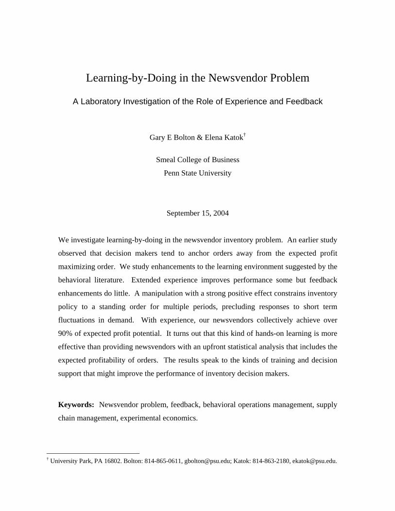
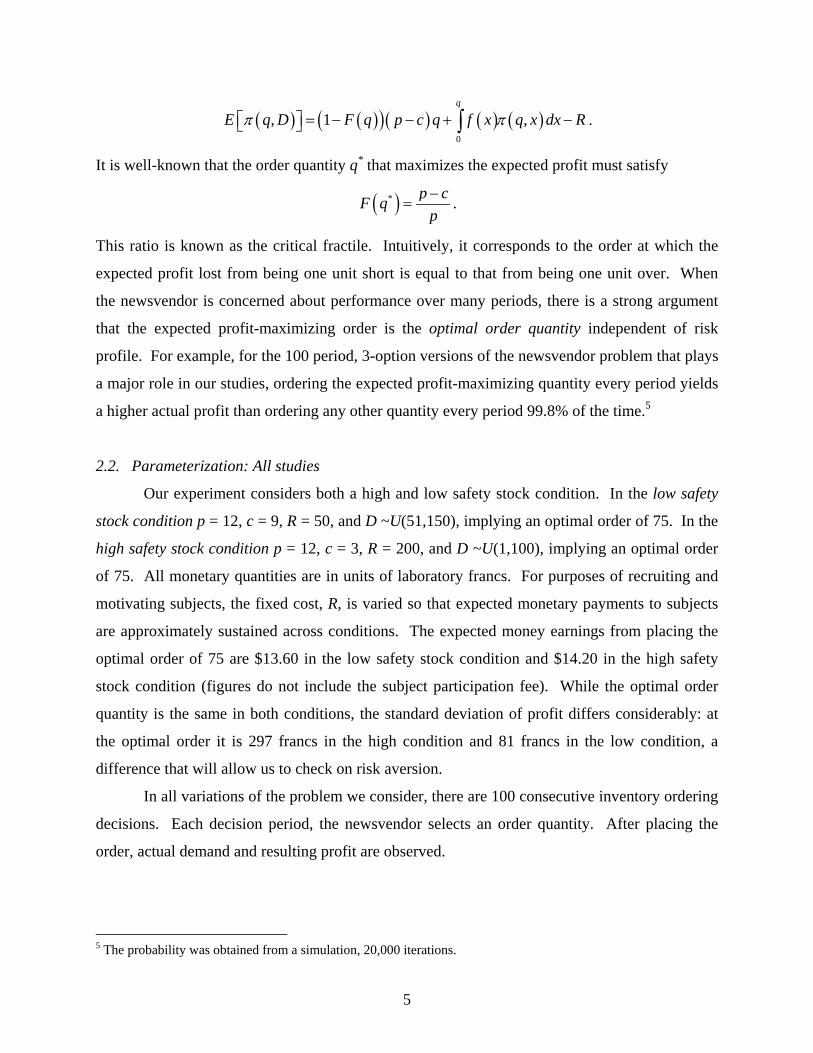
Figure 1 – Expected profit as a function of order quantity. The expected profit function flattens about the optimums at 75. The gray lines mark the three order options in the 3-option conditions (described below).

Schweitzer and Cachon gave their subjects 30 periods of experience and found little

improvement in performance. A straightforward hypothesis is that newsvendors need extended

experience to learn the optimal solution. We extend experience for our subjects to 100 periods.

Experience hypothesis. With extended experience, newsvendors move away from average

demand and towards the optimal order quantity.

Extended experience provides newsvendors with greater opportunity to experiment with

ordering policy. There are, however, reasons to wonder whether this extra experience will be

useful. Observe from Figure 1 that the expected profit curve for the newsvendor problem is non-

linear and flattens substantially as the order quantity approaches the optimal order. To see the

problem this flattening might cause, suppose that a newsvendor in the low condition initially

orders the average demand but then experiments by incrementally ordering less, moving towards

the optimum. As the newsvendor climbs the expected profit function, incremental gains to

expected profit become smaller and at some point perhaps no longer salient. The newsvendor

stops experimenting under the false impression that the optimum has been reached.

The importance of salience is established in the experimental economics literature.

Harrison (1989) demonstrates that first-price auction bidders’ failure to adjust their bids to the

optimum could be attributed to an expected payoff function that is relatively flat about the

optimum bid. Erev and Roth’s (1998) reinforcement learning model provides some theoretical

foundation. In their model, agents learn more quickly when the higher the gains to doing so.

7

Returning to Figure 1, observe that the expected amount to be gained from moving from

ordering average demand all the way to ordering the optimum is quite substantial – the many

small increments add up. A simple way of testing the salience conjecture would be to thin the

ordering space, making the step increments larger. Fewer choices also make it easier to organize

feedback and detect differences in performance.

3.1 Study 1 treatments and laboratory implementation

In study 1, we compare the 100-options games to 9-options games and to 3-option games.

We conduct each of these three treatments for both high and low safety stock parameterizations,

for a 3 x 2 design. Procedures are as given in sections 2.2 and 2.3.

For the low safety stock condition, the 100-options were the integers from 51 to 150, and

the 9-options were 75, 80, 85, 90, 95, 100, 105, 110, and 115. In the 3-option case, newsvendors

choose between 75, 100 and 115; the latter because 125, the midway between 100 and 150,

yields an easily detected negative expected profit, making for what is effectively a 2-option

game.6 Treatments for the high safety stock condition are analogous: the 100-options were the

integers from 1 to 100, the 9-options were 35, 40, 45, 50, 55, 60, 65, 70, and 75, and the 3-

options were 35, 50 and 75.

Each treatment had 20 subjects save 100-option, high safety stock which had 18.

50

60

70

80

90

100

110

120

130

140

150

1 2 3 4 5 6 7 8 9 10

10-decision block

Uni

ts

Avg. Order +- St dev Optimal Avg. Demand

0

10

20

30

40

50

60

70

80

90

100

1 2 3 4 5 6 7 8 9 10

10-decision block

Uni

ts

Avg. Order +- St dev Optimal Avg. Demand

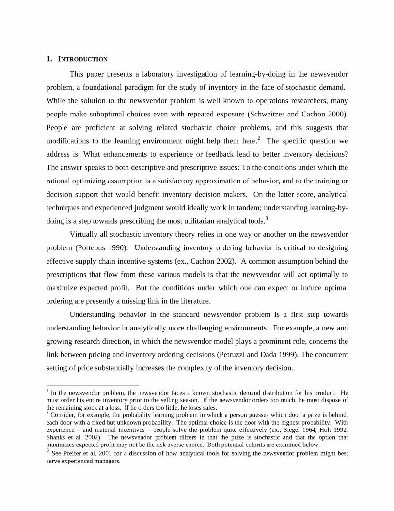
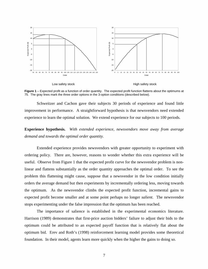
Low safety stock High safety stock Figure 2 – Actual average orders, optimal orders and average demand in the 100-option treatments. Average orders are, in both treatments, between the optimal order quantity and the average demand.

6 Three is the minimum number of options that satisfy criteria important to distinguishing behavioral hypotheses: For example, distinguishing between average demand matching and a preference for minimizing variability requires a third option. Also, the optimal order is an extreme choice in the 3 and 9-option conditions but not in the 100-option condition, and this allows a check whether subjects are averse to selecting an extreme option; the interested reader can verify, from the data displays below, that this does not seem to be the case.

8

3.2 Study 1 results

For the purpose of exposition, we take as baselines the 100-option treatments. These

treatments are the most similar to those in Schweitzer and Cachon’s and serve to benchmark our

experimental apparatus with theirs. Also, the 100-option, high safety stock treatment uses

executive MBAs, providing a benchmark for results obtained with undergraduates against a

subject pool with managerial experience.

For the 100-option conditions, we observe the same pattern of anchoring and insufficient

adjustment that Schweitzer and Cachon observed. From Figure 2, for both low and high safety

stock conditions, the average order stays between average demand and the optimal order

quantity. The average order across individuals and periods in the low condition is 88 and for the

high condition it is 61, both significantly different than 75 (both Wilcoxon, two-tailed p < 0.001).

Risk aversion would pull orders below 75, contrary to what we see in the low profit condition.

Figure 2 also exhibits trends towards the optimal order (OLS, two-sided p < 0.001 in both

cases), confirming the extended experience hypothesis. But the trend emerges slowly; like

Schweitzer and Cachon, little trend is apparent in the first 30 periods. The average for the final

10-period decision block is weakly significantly different from the optimum order (Wilcoxon,

two-tailed p = 0.089), and strongly so for the low condition (p = 0.002). The trend is somewhat

more pronounced in the high condition (two-tailed p = 0.0605). This is plausibly due to the

executive MBAs in the high condition (some other differences may also play a role7). But even

with executives, the improvement is gradual. Also, the standard deviations of orders are quite

high for both conditions, indicating a good deal of variation in between subject ordering even

with extended experience (Figure 2). So while extended experience helps, there is room for

improvement.

We move now to a comparison of performance as the option set thins and the salience of

the remaining options increases. Here we measure performance by the expected profit associated

with each choice; the metric gives answers that are comparable to those obtained by looking

directly at order quantities (Figure 2) with the advantage that it provides a comparison to the

7 Executive MBAs played in a classroom where information may have been shared in spite of requests that it not be, prizes were paid to only the best performer although all performances were open to ex post classroom discussion, and executive MBAs each received a different random demand draw (although the demand draw used for the other treatments shows no apparent anomaly). Schweitzer and Cachon observe better performance in their high treatment with a uniform subject pool, and posit that holding high safety stock is more intuitive than a low safety stock.

9

0.5

0.6

0.7

0.8

0.9

1.0

100-option 9-option 3-option

Pro

porti

on o

f Max

Exp

ecte

d P

rofit

Low safety stock High safety stock

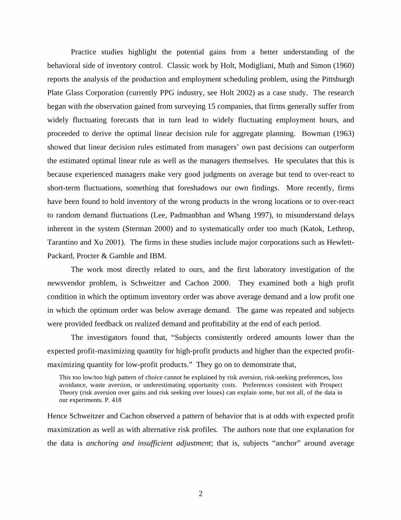
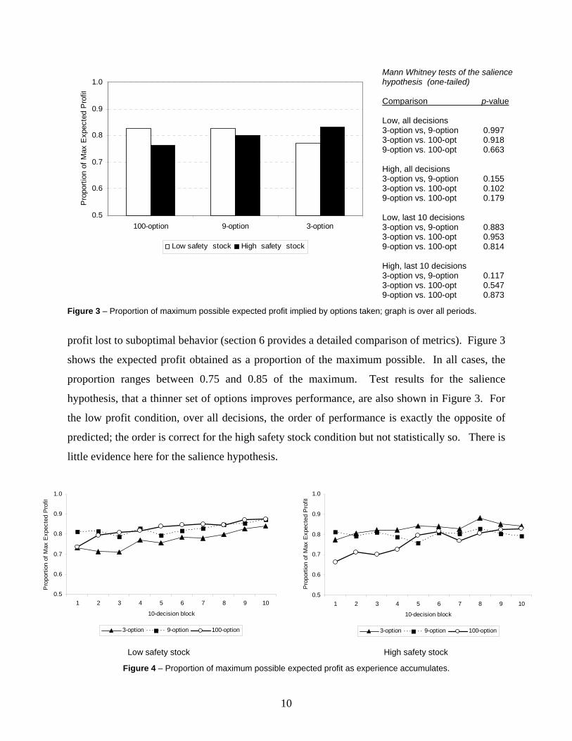
Mann Whitney tests of the salience hypothesis (one-tailed) Comparison p-value Low, all decisions 3-option vs, 9-option 0.997 3-option vs. 100-opt 0.918 9-option vs. 100-opt 0.663 High, all decisions 3-option vs, 9-option 0.155 3-option vs. 100-opt 0.102 9-option vs. 100-opt 0.179 Low, last 10 decisions 3-option vs, 9-option 0.883 3-option vs. 100-opt 0.953 9-option vs. 100-opt 0.814 High, last 10 decisions 3-option vs, 9-option 0.117 3-option vs. 100-opt 0.547 9-option vs. 100-opt 0.873

Figure 3 – Proportion of maximum possible expected profit implied by options taken; graph is over all periods.

profit lost to suboptimal behavior (section 6 provides a detailed comparison of metrics). Figure 3

shows the expected profit obtained as a proportion of the maximum possible. In all cases, the

proportion ranges between 0.75 and 0.85 of the maximum. Test results for the salience

hypothesis, that a thinner set of options improves performance, are also shown in Figure 3. For

the low profit condition, over all decisions, the order of performance is exactly the opposite of

predicted; the order is correct for the high safety stock condition but not statistically so. There is

little evidence here for the salience hypothesis.

0.5

0.6

0.7

0.8

0.9

1.0

1 2 3 4 5 6 7 8 9 10

10-decision block

Pro

porti

on o

f Max

Exp

ecte

d P

rofit

3-option 9-option 100-option

0.5

0.6

0.7

0.8

0.9

1.0

1 2 3 4 5 6 7 8 9 10

10-decision block

Pro

porti

on o

f Max

Exp

ecte

d P

rofit

3-option 9-option 100-option

Low safety stock High safety stock

Figure 4 – Proportion of maximum possible expected profit as experience accumulates.

10

Still, we might expect a salience effect to become evident with experience. Figure 4

shows how expected profit evolves across 10-period blocks for each of the three treatments.

Observe a positive experience effect on performance in all cases save 9-option high safety stock;

formal statistical tests bear this out.8 By the last 10-decision blocks, there are some differences

in expected profit across treatments but most go in the opposite direction of the salience

hypothesis (Figure 3). Hence, salience has no systematic effect even with experience.

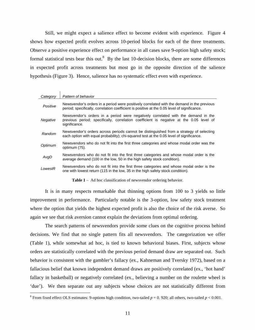
Category Pattern of behavior

Positive Newsvendor’s orders in a period were positively correlated with the demand in the previous period; specifically, correlation coefficient is positive at the 0.05 level of significance.

Negative Newsvendor’s orders in a period were negatively correlated with the demand in the previous period; specifically, correlation coefficient is negative at the 0.05 level of significance.

Random Newsvendor’s orders across periods cannot be distinguished from a strategy of selecting each option with equal probability); chi-squared test at the 0.05 level of significance.

Optimum Newsvendors who do not fit into the first three categories and whose modal order was the optimum (75).

AvgD Newsvendors who do not fit into the first three categories and whose modal order is the average demand (100 in the low, 50 in the high safety stock condition).

LowestR Newsvendors who do not fit into the first three categories and whose modal order is the one with lowest return (115 in the low, 35 in the high safety stock condition).

Table 1 – Ad hoc classification of newsvendor ordering behavior.

It is in many respects remarkable that thinning options from 100 to 3 yields so little

improvement in performance. Particularly notable is the 3-option, low safety stock treatment

where the option that yields the highest expected profit is also the choice of the risk averse. So

again we see that risk aversion cannot explain the deviations from optimal ordering.

The search patterns of newsvendors provide some clues on the cognitive process behind

decisions. We find that no single pattern fits all newsvendors. The categorization we offer

(Table 1), while somewhat ad hoc, is tied to known behavioral biases. First, subjects whose

orders are statistically correlated with the previous period demand draw are separated out. Such

behavior is consistent with the gambler’s fallacy (ex., Kahneman and Tversky 1972), based on a

fallacious belief that known independent demand draws are positively correlated (ex., ‘hot hand’

fallacy in basketball) or negatively correlated (ex., believing a number on the roulette wheel is

‘due’). We then separate out any subjects whose choices are not statistically different from 8 From fixed effect OLS estimates: 9-options high condition, two-tailed p = 0. 920; all others, two-tailed p < 0.001.

11

arbitrary random. Remaining subjects are classified by modal behavior: Optimum, if the most

prevalent action was the optimum order; AvgD if it was average demand; and LowestR if the

modal choice was the strategy with lowest expected return.

0.0

0.1

0.2

0.3

0.4

0.5

0.6

0.7

0.8

0.9

1.0

Positive Negative Random Optimum AvgD Low estR

Classif ication

Prop

ortio

n of

sub

ject

s

Low safety stock High safety stock

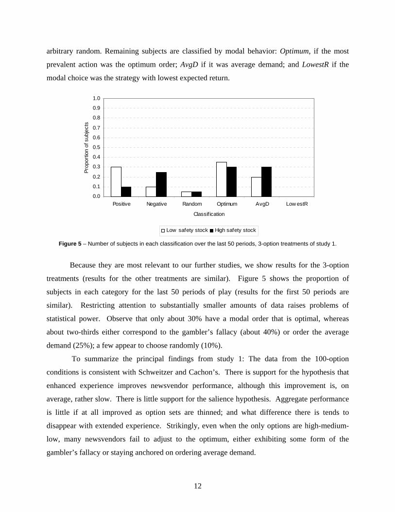
Figure 5 – Number of subjects in each classification over the last 50 periods, 3-option treatments of study 1.

Because they are most relevant to our further studies, we show results for the 3-option

treatments (results for the other treatments are similar). Figure 5 shows the proportion of

subjects in each category for the last 50 periods of play (results for the first 50 periods are

similar). Restricting attention to substantially smaller amounts of data raises problems of

statistical power. Observe that only about 30% have a modal order that is optimal, whereas

about two-thirds either correspond to the gambler’s fallacy (about 40%) or order the average

demand (25%); a few appear to choose randomly (10%).

To summarize the principal findings from study 1: The data from the 100-option

conditions is consistent with Schweitzer and Cachon’s. There is support for the hypothesis that

enhanced experience improves newsvendor performance, although this improvement is, on

average, rather slow. There is little support for the salience hypothesis. Aggregate performance

is little if at all improved as option sets are thinned; and what difference there is tends to

disappear with extended experience. Strikingly, even when the only options are high-medium-

low, many newsvendors fail to adjust to the optimum, either exhibiting some form of the

gambler’s fallacy or staying anchored on ordering average demand.

12

4. STUDY 2: TRACKING PERFORMANCE The patterns of behavior evident in Figure 5 suggest two potential remedies. In study 2,

we investigate giving people feedback about the payoffs associated with options not taken as

well as taken. Doing so might speed the experience effect and might also make it easier for

people to see the futility of demand chasing. We work with the 3-option game, the thinned

option space making it easier to process the option information we will introduce. 9 The other,

more invasive approach would be to constrain inventory policy away from misguided behavior

such as the gambler’s fallacy, the subject of study 3, section 5.

There is both theory and data to suggest that feedback on foregone options can help

learning, at least for certain decision tasks. Learning from foregone options is the basis of

fictitious play learning models (Brown 1951). Models that combine this sort of learning with

reinforcement learning fit observed behavior from a variety of games such as coordination games

(ex., Camerer and Ho 1999).

Tracking hypothesis. Profitability information for options that have not been chosen should

improve performance through faster learning.

We will see that, for the newsvendor problem, the tracking hypothesis has but limited validity.

As a consequence, we also explore giving subjects feedback that has been massaged, in the form

of a 10-period moving average. The idea is that the moving average smoothes much of the

variability in single period feedback. It also moves us in the direction of introducing analysis

tools to be used in tangent with experience and feedback. 4.1 Study 2 treatments and laboratory implementation

Procedures are given in sections 2.2 and 2.3. The only changes made to the 3-option

games described in section 3.1 concern displays for the additional information. Information

concerning the payoff to foregone option for the most recent decision was added to the blue pop-

up box (shown in Appendix), while for older decisions this information was displayed in the

history box (also shown in the appendix). The necessary additional information for the moving

average treatment was added in an analogous way. 9 Schweitzer and Cachon gave their subjects extensive tables showing all possible profit outcomes for each possible inventory order (but not expected values or other statistical analysis). So in principle, subjects had access for foregone payoff information. However, subjects’ had to actively access this information. Also, this information might arguably be more effective when attention is restricted to 3 options.

13

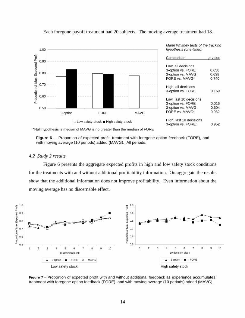
Each foregone payoff treatment had 20 subjects. The moving average treatment had 18.

0.50

0.60

0.70

0.80

0.90

1.00

3-option FORE MAVG

Pro

porti

on o

f Max

Exp

ecte

d P

rofit

Low safety stock High safety stock

Mann Whitney tests of the tracking hypothesis (one-tailed) Comparison p-value Low, all decisions 3-option vs. FORE 0.658 3-option vs. MAVG 0.638 FORE vs. MAVG* 0.740 High, all decisions 3-option vs. FORE 0.169 Low, last 10 decisions 3-option vs. FORE 0.016 3-option vs. MAVG 0.604 FORE vs. MAVG* 0.932 High, last 10 decisions 3-option vs. FORE: 0.952

*Null hypothesis is median of MAVG is no greater than the median of FORE Figure 6 – Proportion of expected profit, treatment with foregone option feedback (FORE), and with moving average (10 periods) added (MAVG). All periods.

4.2 Study 2 results

Figure 6 presents the aggregate expected profits in high and low safety stock conditions

for the treatments with and without additional profitability information. On aggregate the results

show that the additional information does not improve profitability. Even information about the

moving average has no discernable effect.

0.5

0.6

0.7

0.8

0.9

1.0

1 2 3 4 5 6 7 8 9 10

10-decision block

Pro

porti

on o

f Max

Exp

ecte

d P

rofit

3-option FORE MAVG

0.5

0.6

0.7

0.8

0.9

1.0

1 2 3 4 5 6 7 8 9 10

10-decision block

Pro

porti

on o

f Max

Exp

ecte

d P

rofit

3-option FORE

Low safety stock High safety stock

Figure 7 – Proportion of expected profit with and without additional feedback as experience accumulates, treatment with foregone option feedback (FORE), and with moving average (10 periods) added (MAVG).

14

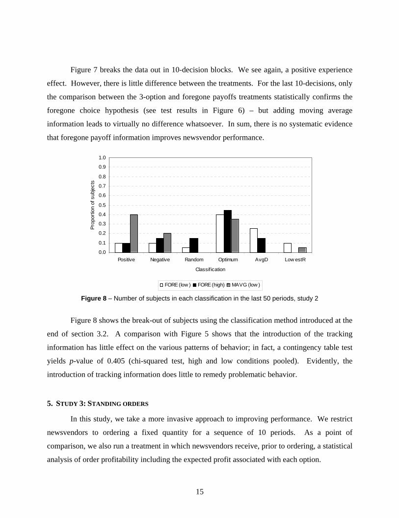
Figure 7 breaks the data out in 10-decision blocks. We see again, a positive experience

effect. However, there is little difference between the treatments. For the last 10-decisions, only

the comparison between the 3-option and foregone payoffs treatments statistically confirms the

foregone choice hypothesis (see test results in Figure 6) – but adding moving average

information leads to virtually no difference whatsoever. In sum, there is no systematic evidence

that foregone payoff information improves newsvendor performance.

0.0

0.1

0.2

0.3

0.4

0.5

0.6

0.7

0.8

0.9

1.0

Positive Negative Random Optimum AvgD Low estR

Classification

Prop

ortio

n of

sub

ject

s

FORE (low ) FORE (high) MAVG (low )

Figure 8 – Number of subjects in each classification in the last 50 periods, study 2

Figure 8 shows the break-out of subjects using the classification method introduced at the

end of section 3.2. A comparison with Figure 5 shows that the introduction of the tracking

information has little effect on the various patterns of behavior; in fact, a contingency table test

yields p-value of 0.405 (chi-squared test, high and low conditions pooled). Evidently, the

introduction of tracking information does little to remedy problematic behavior.

5. STUDY 3: STANDING ORDERS

In this study, we take a more invasive approach to improving performance. We restrict

newsvendors to ordering a fixed quantity for a sequence of 10 periods. As a point of

comparison, we also run a treatment in which newsvendors receive, prior to ordering, a statistical

analysis of order profitability including the expected profit associated with each option.

15

0

0.5

1

1.5

2

2.5

3

3.5

4

4.5

5

-500 -400 -300 -200 -100 0 100 200 300 400 500

average

freq.

, 10^

-3

0

0.5

1

1.5

2

2.5

3

3.5

4

4.5

5

-500 -400 -300 -200 -100 0 100 200 300 400 500

average

freq.

, 10^

-3

n = 3 n = 10

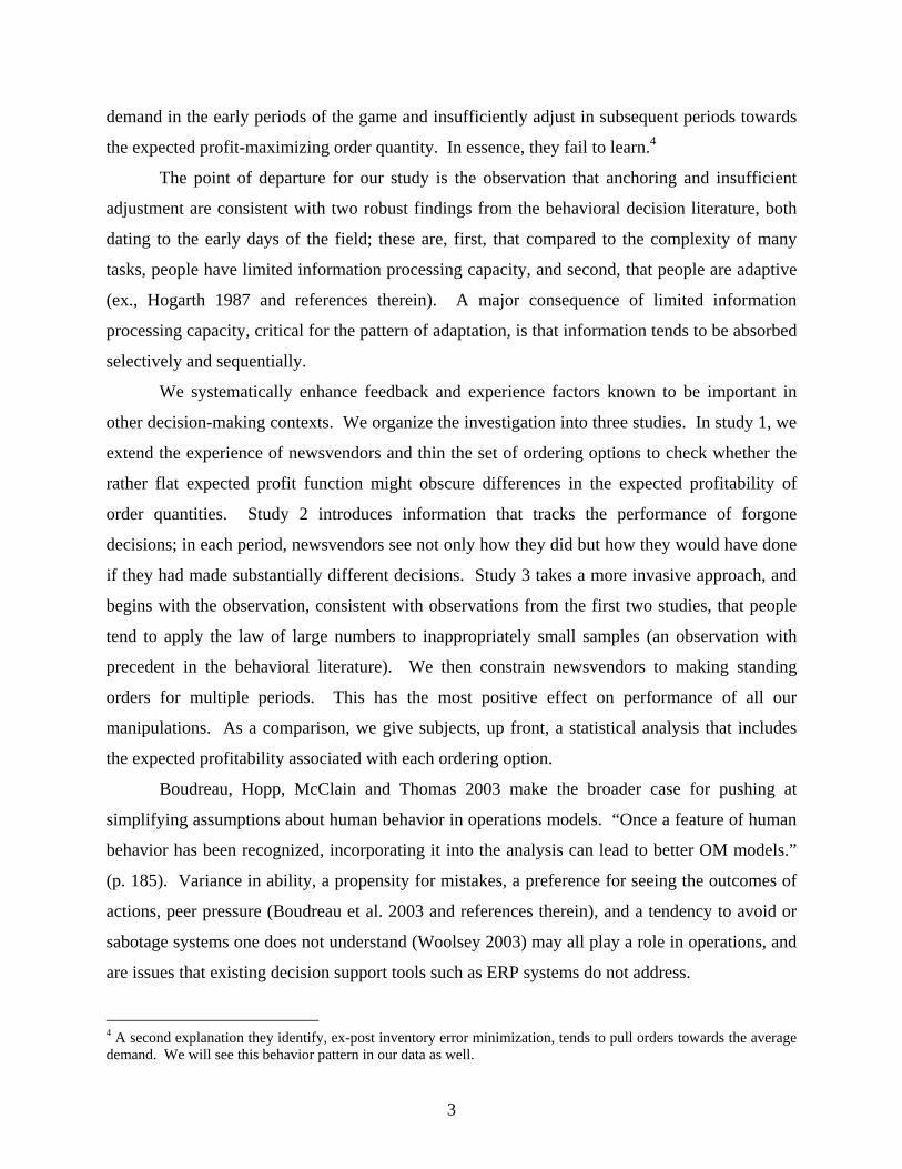
Figure 9 – High safety stock, 3-options. Simulations of sampling distributions for ordering 75 for sample size n, simulation iterations = 20,000. Both distributions have a mean of 93. For n=3, the standard deviation is 169.5; for n=10 it falls to 93.3.

Learning-by-doing in the newsvendor problem involves sampling and exploiting the law

of large numbers. Kahneman and Tversky 1971 show that many people seem to believe in a

‘law of small numbers’, that small samples are representative as well as large. Consistent with

this, many newsvendors in our sample jump too quickly to draw accurate conclusions about the

optimum order’s expected profitability; for example, for newsvendors not classified as Optimum

in Figure 8, the average sample run for the optimum order is 2.4 consecutive orders, with a

median and mode of 1. This might explain why some tend to stick to the expected demand

anchor for so long (cursory sampling of other orders turns up little that is positive) as well as

why others’ orders are correlated with demand (a small number of demand observations leads

them to believe another order is more profitable). Through this lens, the correlated behavior is

likened to ‘day trading’, the short-term trading of stocks on the fallacy that one can predict future

market fluctuations.

Day trading hypothesis. Restricting newsvendors to longer term policy induces more

representative sampling, and impedes short term market chasing. The basic manipulation in study 3 restricts newsvendors to ordering a fixed amount for a

run of 10 periods, thereby forcing newsvendors to draw a sample of size 10 each time they

choose to sample an order. To get a sense of how much more informative this is than what

people typically do, Figure 9 compares the sampling distributions of 3-consecutive orders with

10-consecutive orders. The standard error for a sample of 10 is about half that for a sample of 3.

16

5.1 Study 3 treatments and laboratory implementation

Procedures are given in sections 2.2 and 2.3. In study 3, newsvendors order for 10

periods at a time. We collect data for 100 orders, so newsvendors participate in 1000 demand

draws (the first 100 draws were the same as in the comparable low and high safety stock

treatments). After ordering, newsvendors observed the average performance over the 10 periods

of both the option chosen as well as those not chosen; this information was presented in an

analogous way to information in study 2 (section 4.1). We also conducted a low safety stock

treatment in which subjects were given, at the beginning of the session, a sheet with the expected

profit associated with each option, as well as the range of profit. This full accounting of

profitability (as opposed to simply stating the expected profit) was intended to avoid leading the

subjects ( “demand effects” in laboratory parlance) and makes the variability of profit associated

with each option clear (sample chart in Appendix). We also gave subjects foregone payoff

feedback (but not the moving average). For baselines we use the foregone payoff treatments of

study 2, although our conclusions are robust to other choices (see section 6).

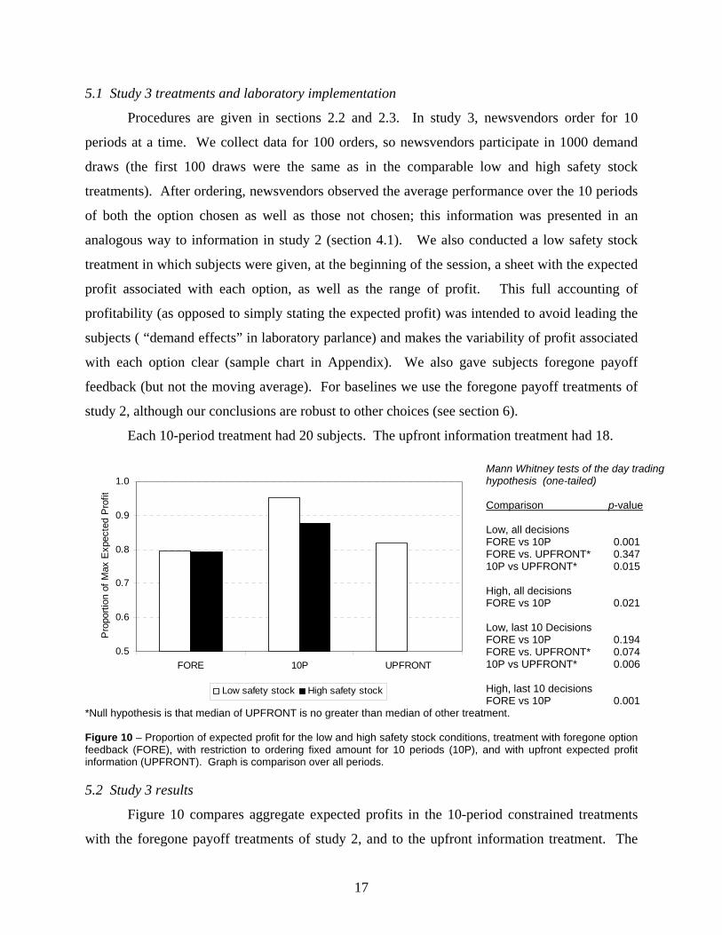
Each 10-period treatment had 20 subjects. The upfront information treatment had 18.

0.5

0.6

0.7

0.8

0.9

1.0

FORE 10P UPFRONT

Pro

porti

on o

f Max

Exp

ecte

d P

rofit

Low safety stock High safety stock

Mann Whitney tests of the day tradinghypothesis (one-tailed) Comparison p-value Low, all decisions FORE vs 10P 0.001 FORE vs. UPFRONT* 0.347 10P vs UPFRONT* 0.015 High, all decisions FORE vs 10P 0.021 Low, last 10 Decisions FORE vs 10P 0.194 FORE vs. UPFRONT* 0.074 10P vs UPFRONT* 0.006 High, last 10 decisions FORE vs 10P 0.001

*Null hypothesis is that median of UPFRONT is no greater than median of other treatment. Figure 10 – Proportion of expected profit for the low and high safety stock conditions, treatment with foregone option feedback (FORE), with restriction to ordering fixed amount for 10 periods (10P), and with upfront expected profit information (UPFRONT). Graph is comparison over all periods. 5.2 Study 3 results

Figure 10 compares aggregate expected profits in the 10-period constrained treatments

with the foregone payoff treatments of study 2, and to the upfront information treatment. The

17

10-period constrained treatments have a clear effect at all standard levels of significance.

Upfront information, while improving performance a bit, has no statistically significant effect.

0.5

0.6

0.7

0.8

0.9

1.0

1 2 3 4 5 6 7 8 9 10

10-decision block

Pro

porti

on o

f Max

Exp

ecte

d P

rofit

FORE 10P UPFRONT

0.5

0.6

0.7

0.8

0.9

1.0

1 2 3 4 5 6 7 8 9 10

10-decision block

Pro

porti

on o

f Max

Exp

ecte

d P

rofit

FORE 10P

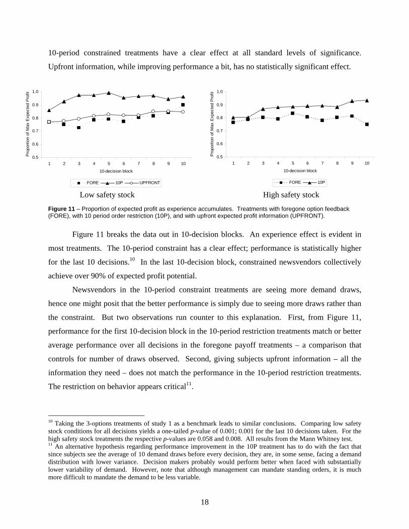
Low safety stock High safety stock Figure 11 – Proportion of expected profit as experience accumulates. Treatments with foregone option feedback (FORE), with 10 period order restriction (10P), and with upfront expected profit information (UPFRONT).

Figure 11 breaks the data out in 10-decision blocks. An experience effect is evident in

most treatments. The 10-period constraint has a clear effect; performance is statistically higher

for the last 10 decisions.10 In the last 10-decision block, constrained newsvendors collectively

achieve over 90% of expected profit potential.

Newsvendors in the 10-period constraint treatments are seeing more demand draws,

hence one might posit that the better performance is simply due to seeing more draws rather than

the constraint. But two observations run counter to this explanation. First, from Figure 11,

performance for the first 10-decision block in the 10-period restriction treatments match or better

average performance over all decisions in the foregone payoff treatments – a comparison that

controls for number of draws observed. Second, giving subjects upfront information – all the

information they need – does not match the performance in the 10-period restriction treatments.

The restriction on behavior appears critical11.

10 Taking the 3-options treatments of study 1 as a benchmark leads to similar conclusions. Comparing low safety stock conditions for all decisions yields a one-tailed p-value of 0.001; 0.001 for the last 10 decisions taken. For the high safety stock treatments the respective p-values are 0.058 and 0.008. All results from the Mann Whitney test. 11 An alternative hypothesis regarding performance improvement in the 10P treatment has to do with the fact that since subjects see the average of 10 demand draws before every decision, they are, in some sense, facing a demand distribution with lower variance. Decision makers probably would perform better when faced with substantially lower variability of demand. However, note that although management can mandate standing orders, it is much more difficult to mandate the demand to be less variable.

18

0.0

0.1

0.2

0.3

0.4

0.5

0.6

0.7

0.8

0.9

1.0

Positive Negative Random Optimum AvgD Low estR

Classif ication

Prop

ortio

n of

sub

ject

s

10P (low ) UPFRONT (low ) 10P (high)

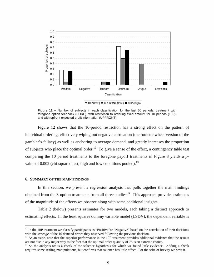
Figure 12 – Number of subjects in each classification for the last 50 periods, treatment with foregone option feedback (FORE), with restriction to ordering fixed amount for 10 periods (10P), and with upfront expected profit information (UPFRONT).

Figure 12 shows that the 10-period restriction has a strong effect on the pattern of

individual ordering, effectively wiping out negative correlation (the roulette wheel version of the

gambler’s fallacy) as well as anchoring to average demand, and greatly increases the proportion

of subjects who place the optimal order.12 To give a sense of the effect, a contingency table test

comparing the 10 period treatments to the foregone payoff treatments in Figure 8 yields a p-

value of 0.002 (chi-squared test, high and low conditions pooled).13

6. SUMMARY OF THE MAIN FINDINGS

In this section, we present a regression analysis that pulls together the main findings

obtained from the 3-option treatments from all three studies.14 This approach provides estimates

of the magnitude of the effects we observe along with some additional insights.

Table 2 (below) presents estimates for two models, each taking a distinct approach to

estimating effects. In the least squares dummy variable model (LSDV), the dependent variable is

12 In the 10P treatment we classify participants as “Positive”or “Negative” based on the correlation of their decisions with the average of the 10 demand draws they observed following the previous decision. 13 As an aside, note that the superior performance in the 10P treatment provides additional evidence that the results are not due in any major way to the fact that the optimal order quantity of 75 is an extreme choice. 14 So the analysis omits a check of the salience hypothesis for which we found little evidence. Adding a check requires some scaling manipulations, but confirms that salience has little effect. For the sake of brevity we omit it.

19

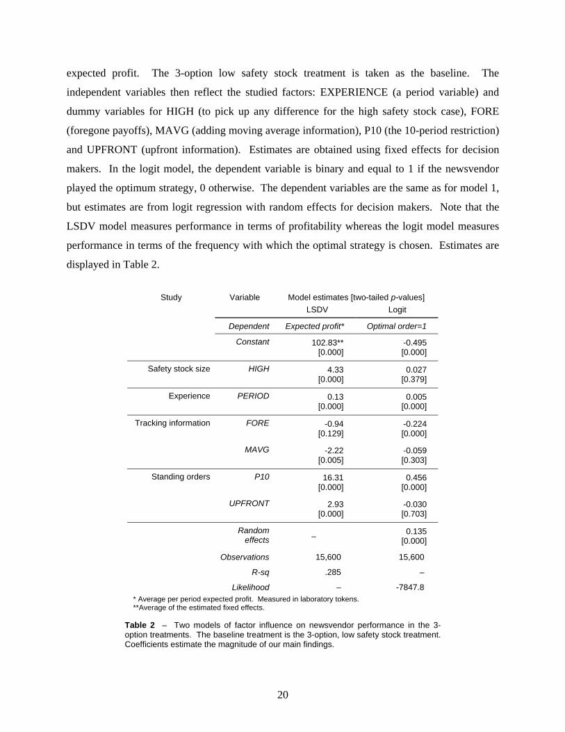
expected profit. The 3-option low safety stock treatment is taken as the baseline. The

independent variables then reflect the studied factors: EXPERIENCE (a period variable) and

dummy variables for HIGH (to pick up any difference for the high safety stock case), FORE

(foregone payoffs), MAVG (adding moving average information), P10 (the 10-period restriction)

and UPFRONT (upfront information). Estimates are obtained using fixed effects for decision

makers. In the logit model, the dependent variable is binary and equal to 1 if the newsvendor

played the optimum strategy, 0 otherwise. The dependent variables are the same as for model 1,

but estimates are from logit regression with random effects for decision makers. Note that the

LSDV model measures performance in terms of profitability whereas the logit model measures

performance in terms of the frequency with which the optimal strategy is chosen. Estimates are

displayed in Table 2.

Study Variable Model estimates [two-tailed p-values]

LSDV Logit

Dependent Expected profit* Optimal order=1

Constant 102.83** [0.000]

-0.495 [0.000]

Safety stock size HIGH 4.33 [0.000]

0.027 [0.379]

Experience PERIOD 0.13 [0.000]

0.005 [0.000]

Tracking information FORE -0.94 [0.129]

-0.224 [0.000]

MAVG -2.22 [0.005]

-0.059 [0.303]

Standing orders P10 16.31 [0.000]

0.456 [0.000]

UPFRONT 2.93 [0.000]

-0.030 [0.703]

Random effects – 0.135

[0.000]

Observations 15,600 15,600

R-sq .285 –

Likelihood – -7847.8 * Average per period expected profit. Measured in laboratory tokens. **Average of the estimated fixed effects.

Table 2 – Two models of factor influence on newsvendor performance in the 3-option treatments. The baseline treatment is the 3-option, low safety stock treatment. Coefficients estimate the magnitude of our main findings.

20

The major observations in Table 2 are these:

All other things equal, newsvendors do better in the high safety stock condition than in

the low safety stock condition. We see from the LSDV model that, on average, newsvendors

capture more of the expected profit potential. Interestingly, the logit model shows that this is not

because they, in any meaningful way, order the optimal amount more often. Schweitzer and

Cachon also found that newsvendor do better in the high condition. They speculated that this

might be because the optimal order in the low condition (holding less than average demand) is

less intuitive to newsvendors than the optimal order in the high condition. This explanation is

consistent with our logit finding: It turns out that newsvendors in the high condition do better

because newsvendors in the low condition more often order the poorest expected profit option.15

Experience improves performance. Holding all other factors fixed, experience improves

profit performance and increases the probability that newsvendors will make the optimal order.

Performance tracking information alone does not improve performance. The regressions

confirm our finding that there is no detectable effect from adding information about foregone

options, including showing the moving averages.

Restricting ordering to standing orders for 10 periods improves performance both in

terms of expected profit potential exploited and in terms of making the optimal order. We can

see in the regressions that this constraint easily has the biggest impact of any factor studied.

Also, newsvendors who learn by doing in this way do better than those given the statistical

analysis upfront.

7. CONCLUSIONS AND MANAGERIAL IMPLICATIONS

The newsvendor problem is difficult for most people to solve even with the simple

demand structure featured in our experiment. Learning-by-doing in the field is likely to be at

least as difficult since information about demand distributions in actual business environments is

often sketchy with the distribution changing over time in ways that can be difficult to assess.

Experiential judgments are bound to be important because analytical techniques, as helpful as

they are, are also limited in capability.

15 Tabulating the data, newsvendors in the low, 3-option treatment are 50% more likely to place the lowest expected profit order than are newsvendors in the high, 3-option treatment. Introducing foregone payoff information reduces the gap to a still substantial 20%

21

Our findings imply three managerial insights for learning by doing inventory ordering:

Procedures and incentives for inventory decision makers should focus on long-term

trends, restraining responses to short-term fluctuations. Tools for supply chain coordination and

information sharing, such as ERP, have the potential for generating a great deal of data, but what

information is likely to be useful for improving performance? Our results imply that

constraining decision-makers from responding to short-term trends can improve performance.

Decision-makers over-react to short-term fluctuations, losing track of the long term picture.

Knowledge gained from hands-on experience is more readily utilized than knowledge

gained from a third party source. The idea that experience can overwrite pre-conceived biases

more effectively than knowledge gained from third party sources has implications for designing

training programs. Our results suggest that the most effective type of employee training would

contain an experiential component to make its points. The idea of a “management flight

simulator” proposed by Sterman (1989) (the “beer distribution game” is an example) is

consistent with this view. Information delivered without an experiential context, like the

expected profit distribution information in Study 3, is more likely to be ignored or disregarded

than the same information gained by personal experience.

Sensible restriction of the options before the decision maker enables more targeted

feedback and hence more effective learning-by-doing. Just as information overload can degrade

performance, so can too many options. While we found that limiting the number of options

available to the decision-maker by itself did little, the limitation provided the canvas for more

targeted learning-by-doing, gathering and organizing a more manageable amount of information.

Of course the question of how to limit options in a way that does not eliminate good decisions is

an important and potentially difficult one. But one implication of our study is that careful

consideration of what options can be safely eliminated a priori can be a worthwhile investment.

The simplicity of the stochastic demand structure of the present experiment is also

arguably its greatest limitation. It may be that the uniform distribution, with its high variance,

actually over-states the problem relative to what we would expect to observe in practice. On the

other hand, demand distributions in practice are never known with certainty. It would be

interesting to see how experience and restricting to standing orders do in an environment where

the demand distribution is more complex or its character less certain. On this we hope to have

something to say soon.

22

APPENDIX. SAMPLE MATERIALS FOR THE EXPERIMENT Written instructions given to subjects for the 3-option, high safety stock treatment. General. The purpose of this session is to study how people make decisions in a particular situation. If you have any questions, feel free to raise your hand and a monitor will assist you. From now until the end of the session, unauthorized communication of any nature with other participants is prohibited. During the session you will play a game from which you can earn ‘francs.’ The francs you earn will be converted into U.S. dollars at a rate of 1000 francs per $1. Upon completion of the game, you will be paid your total earnings in U.S. cash plus a $5 show-up fee. Description of the game. You are a retailer who sells a single (fictional) item, the widget. In each round of the game, you order widgets from a supplier at a cost of 3 francs per unit, and sell widgets to your customers at a price of 12 francs per unit. In each round, you also pay a fixed overhead cost (‘rent’) of 200 francs. Your goal is to maximize the profit you make totaled over all the rounds of the game.

In each round, widgets must be ordered from the supplier before you know for certain what quantity your customers will demand. You may order widgets in one of just three quantities: 35, 50 or 75 widgets.

Once you place your order, the computer randomly selects the demand quantity from a range of 1 to 100 units, with each number in the range equally likely. That is, there is a 1/100 chance that demand will be 1, a 1/100 chance that demand will be 2, and so on.

The demand drawn for any one round is independent of the demand from earlier rounds. So a small or large demand in earlier rounds has no influence on whether demand is small or large in later rounds.

Calculating profit. If the number of widgets ordered, W, is the same or less than the quantity demanded, D, then your profit for the round is

Profit = 12W – 3W – 200

For example, if you order 35 widgets and the demand is 60, then your profit for the round is 12(35) – 3(35) - 200 = 115 francs. Note that when the number of widgets ordered is less than demand, you lose opportunities for sales.

If the number of widgets ordered, W, is greater than the quantity demanded, D, then your profit for the round is

Profit = 12D – 3W – 200

For example, if you order 75 widgets and demand is 60, then your profit for the round is 12(45) – 3(75) – 200 = 115 francs. When the number of widgets ordered is greater than demand, you must dispose of the unsold units (widgets go stale after a round, and cannot be carried as inventory into future rounds). Information to help you in your decision. You have been given a sheet that displays the profit you will make for each quantity you could order, and every demand level that might subsequently result. The sheet also provides some summary statistics. A pen and blank sheet of paper have been provided for any calculations of notes you might wish to make. After placing an inventory order, you will receive the demand and profit results for the round. You will also be shown the results that would have occurred if you had ordered either of the other order quantities. The computer will display the history of play (how much you ordered, how much you made) to date. Number of rounds. The game lasts for 100 rounds. Consent Forms. If you wish to participate in this study, please read and sign the accompanying consent form prior to beginning the game.

23

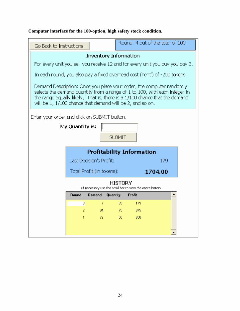
Computer interface for the 100-option, high safety stock condition.

24

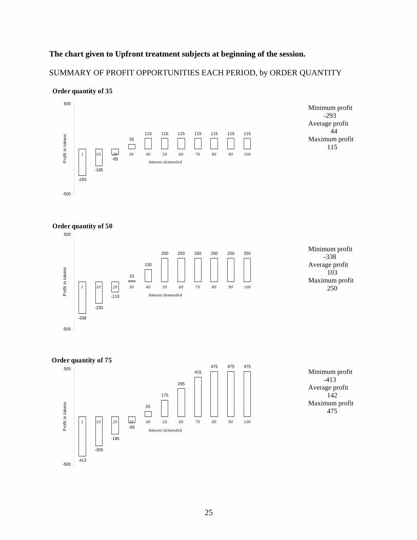
The chart given to Upfront treatment subjects at beginning of the session. SUMMARY OF PROFIT OPPORTUNITIES EACH PERIOD, by ORDER QUANTITY

Order quantity of 35

-293

-185

-65

55115 115 115 115 115 115 115

-500

500

1 10 20 30 40 50 60 70 80 90 100

Amount demandedPro

fit in

toke

ns

Minimum profit -293 Average profit 44 Maximum profit 115

Order quantity of 50

-338

-230

-110

10

130

250 250 250 250 250 250

-500

500

1 10 20 30 40 50 60 70 80 90 100

Amount demandedPro

fit in

toke

ns

Minimum profit -338 Average profit 103 Maximum profit 250

Order quantity of 75

-413

-305

-185

-65

55

175

295

415475 475 475

-500

500

1 10 20 30 40 50 60 70 80 90 100

Amount demandedPro

fit in

toke

ns

Minimum profit -413 Average profit 142 Maximum profit 475

25

ACKNOWLEDGEMENTS

Katok gratefully acknowledges the support of the National Science Foundation, award number SES 0214337. Bolton gratefully acknowledges the support of the National Science Foundation, award number SES 0351408. We thank Gérard Cachon and Maurice Schweitzer for sharing information and materials about their study, and seminar participants at Cornell, the University of Illinois at Urbana-Champaign, and Penn State for insightful comments. REFERENCES

Boudreau, J.W, Hopp, W., McClain, J.O., and Thomas, L.J. (2003), Commissioned paper on the interface between operations and human resources management. Manufacturing & Service Operations Management, Vol 5, No. 3, pp. 179-202.

Bowman, E.H. (1963), Consistency and optimality in managerial decision making. Management

Science, Vol. 9, No. 2, pp. 310-321. Brown, G. (1951), Iterative solution to games by fictitious play, in T. Koopsmans (ed.) Activity

analysis of production and allocation, Wiley: New York. Cachon, G.P. (2002), Supply chain coordination with contracts. S. Graves and Ton de Kok

(Eds.). Handbook in OR & MS, Supply Chain Management. Elsevier, North-Holland. Camerer, C.F. and Teck-Hua Ho. (1999), Experience-weighted Attraction Learning in Normal

Form Games, Econometrica, Vol. 67 (4) pp. 827-874. Croson, R and Karen Donohue. (2002). Experimental economics and supply chain management.

Interfaces Vol. 32, pp.74-82. Croson, R., Donohue, K., Katok, E. and Sterman, J. (2004), Order stability in supply chains: a

behavioral approach. Working Paper, Penn State University. Erev, I. and Roth A.E. (1998), Predicting how people play games: Reinforcement learning in

experimental games with unique mixed strategy equilibria," American Economic Review, 88, 848-881.

Forrester, J., (1958) Industrial dynamics: A major breakthrough for decision makers. Harvard

Business Review, 36, 37-66. Harrison, G.W. (1989), Theory and misbehavior in first-price auctions, American Economic

Review, 79, 749-762. Hogarth, Robin (1987), Judgement and Choice, John Wiley and Sons: New York, 2nd edition. Holt, C.A. (1992), ISO Probability matching. University of Virginia Working Paper.

26

Holt, C.C. (2002), Learning how to plan production, inventories and work force, Operations Research, Vol. 50, No. 1, pp. 96-99.

Holt, C.C., Modigliani, F., Muth, J.F. and Simon, H.A. (1960), Planning Production,

Inventories, and Work Force, Prentice-Hall, Inc., Englewood Cliffs, NJ. Kahneman, D. and Tversky, A. (1972), Subjective probability: A judgment of representativeness,

Cognitive Psychology, 3, 430-454. Kahneman, D. and Tversky, A. (1971), The belief in the law of small numbers, Psychological

Bulletin, 76, 105-110. Katok, E., Lethrop, A., Tarantino, W. and Xu, S.H. (2001), Using dynamic programming-based

DSS to manage inventory at Jeppesen. Interfaces , Vol. 31, No. 6, 54-68. Lee, H., P. Padmanabhan and S. Whang, (1997) Information distortion in a supply chain: the

bullwhip effect. Management Science, 43, 546-558. Petruzzi, N.C. and Dada, M. (1999), Pricing and the newsvendor problem: a review with

extensions. Operations Research Vol. 47, No. 2, pp. 183-194. Pfeifer, Phillip E., Bodily, Samuel E., Carraway, Robert L. Clyman, Dana R. and Frey, Jr.,

Sherwood C. (2001), Preparing out students to be newsvendors, Interfaces. Porteous, E.L. (1990). Stochastic inventory theory. D.P. Heyman and M.J. Sobel (Eds.).

Handbook in OR & MS, Vol 2. Elsevier, North-Holland, 605-652. Rapoport, A. (1966), A study of human control in a stochastic multistage decision task.

Behavioral Sciences, Vol. 11, pp. 18-32. Rapoport, A. (1967), Variables affecting decisions in a multistage inventory task. Behavioral

Sciences, Vol. 12, pp. 194-204. Schultz, K.L., Juran, D.C., Boudreau, J.W., McClain, J.O., and Thomas, L.J. (1998), Modeling

and worker motivation in JIT production systems. Management Science, Vol 44, No. 12, pp. 1595-1607.

Schweitzer, M.E. and Cachon, G.P (2000), Decision bias in the newsvendor problem with known

demand distribution: experimental evidence. Management Science, Vol. 46, pp. 404-420. Shanks, D.R., Tunney, R.J, and McCarthy, J.D. (2002), A re-examination of probability

matching and rational choice. Journal of Behavioral Decision Making, Vol 15, pp. 233-250. Siegel, Sidney (1964), Choice, Strategy, and Utility, McGraw-Hill: New York. Sterman, J., (2000) Business dynamics: systems thinking and modeling for a complex world.

Irwin McGraw-Hill.

27

Sterman, J., (1989), Modeling managerial behavior: misperceptions of feedback in a dynamic

decision making experiment. Management Science, 35, 321-339. Woolsey, R.E.D. (2003), Real world operations research: the Woolsey papers, Hewitt, R.L.

(Ed.), Lionheart Publishing, Inc., Marietta, GA. Wu, Y. and Katok, E. (2004), Can efficient learning mitigate the bullwhip effect? Working

Paper, Penn State University.

28