selling to the ‘‘newsvendor’’ with a forecast...

European Journal of Operational Research 182 (2007) 1150–1176

www.elsevier.com/locate/ejor

Production, Manufacturing and Logistics

Selling to the ‘‘Newsvendor’’ with a forecast update:Analysis of a dual purchase contract q,qq

Ozalp Ozer a,*, Onur Uncu a, Wei Wei b

a Department of Management Science and Engineering, Stanford University, 314 Terman Engineering, Stanford, CA 94305, United Statesb Morgan Stanley, 20 Cabot Square, Canary Warf, London, United Kingdom

Received 5 March 2005; accepted 13 September 2006Available online 13 December 2006

Abstract

We consider a supply chain in which a manufacturer sells to a procure-to-stock retailer facing a newsvendor problemwith a forecast update. Under a wholesale price contract, the retailer waits as long as she can and optimally places herorder after observing the forecast update. We show that the retailer’s wait-and-decide strategy, induced by the wholesaleprice contract, hinders the manufacturer’s ability to (1) set the wholesale price and maximize his profit, (2) hedge againstexcess inventory risk, and (3) reduce his profit uncertainty. To mitigate the adverse effect of wholesale price contract, wepropose the dual purchase contract, through which the manufacturer provides a discount for orders placed before the fore-cast update. We characterize how and when a dual purchase contract creates strict Pareto improvement over a wholesaleprice contract. To do so, we establish the retailer’s optimal ordering policy and the manufacturer’s optimal pricing andproduction policies. We show how the dual purchase contract reduces profit variability and how it can be used as a riskhedging tool for a risk averse manufacturer. Through a numerical study, we provide additional managerial insights andshow, for example, that market uncertainty is a key factor that defines when the dual purchase contract provides strictPareto improvement over the wholesale price contract.� 2006 Elsevier B.V. All rights reserved.

Keywords: Supply chain; Contracting; Advance purchase; Newsvendor model; Forecast updating; Procurement

1. Introduction

In many supply chains, the upstream firm (the manufacturer) must adjust to the downstream firm’s (theretailer’s) demand through continuous refinement of production processes and delivery systems. A well-knownexample from the apparel industry is quick response, a series of process improvement initiatives that enable

0377-2217/$ - see front matter � 2006 Elsevier B.V. All rights reserved.

doi:10.1016/j.ejor.2006.09.057

q The article was previously titled as ‘‘Analysis of a Dual Purchase Contract’’.qq The paper was presented during the 2003 INFORMS Annual Meeting in Atlanta session SD 40, the seminars at Cornell Universityand Stanford University. The authors are grateful for the stimulating discussions.

* Corresponding author. Tel.: +1 650 725 1746.E-mail addresses: [email protected] (O. Ozer), [email protected] (O. Uncu), [email protected] (W. Wei).

mailto:[email protected]



O. Ozer et al. / European Journal of Operational Research 182 (2007) 1150–1176 1151

faster response to retailer orders. Such initiatives allow the retailer to wait until the last possible minute, plac-ing her order after a better forecast becomes available. The practice of last minute ordering is not unique to theapparel industry. A 2002 survey shows that 57% of industrial buyers from automative to electronics increased‘‘just-in-time’’ purchases and reduced buying based on long term forecasts (Ansberry, 2002).

In this paper, we show that last minute ordering and its adverse effect on manufacturers are the resultof a wholesale price contract, which is widely used due to it’s simplicity. Often the procurement con-tract between a manufacturer and a retailer is negotiated well in advance of the sales season, actual ordersand product delivery. Last minute ordering coupled with early commitment to a wholesale price furthersqueezes the manufacturer’s profit. Ansberry (2002, Wall Street Journal) reports anecdotal evidence to con-clude that

‘‘. . . [retailers] are holding onto their cash as long as they can . . . waiting until the last possible moment toensure that every order they place will lead to profits . . . [those] manufacturers receiving last minute ordershave difficulty in justifying equipment purchases. many manufacturers invest in expensive equipment . . . tojustify the cost is to run [the equipment] constantly . . . the system works best when [retailer] places bigorders well in advance . . .’’

The above observations suggest that the consequence of last minute ordering (due to the wholesale pricecontract) to the manufacturer is threefold. First, the manufacturer may not be able to charge the wholesale pricethat maximizes his profit. The negotiation to set the wholesale price often takes place well in advance of the salesseason. Hence, the market potential for the product is uncertain during this negotiation. This uncertaintyhinders the manufacturer’s ability to enforce the optimal wholesale price. Second, last minute orderingnegatively affects the manufacturer’s ability to invest in new technology or justify equipment purchases. Undera wholesale price contract, the retailer delays her ordering decision as much as she can and does not commit tobuying any product prior to obtaining a final forecast update, hence better demand information. The retailerallows just enough time to the manufacturer to produce her orders. The retailer’s wait-and-see strategy,however, requires the manufacturer to invest in production equipment in the face of uncertain profits. Third,the manufacturer often initiates part of his production prior to receiving the retailer’s order when his costs aredecreasing in production lead time. In this case, the manufacturer also faces excess inventory risk.

In this paper, we provide a new contract form with which the manufacturer can (1) push inventory to theretailer, known also as channel stuffing, (2) create a strict Pareto improvement over the wholesale price con-tract while inheriting the wholesale price contract’s simplicity, and (3) reduce the manufacturer’s profit vari-ability. To do so, we propose a dual purchase contract that induces a retailer to place two consecutive orders;before and after obtaining the final forecast update. A dual purchase contract specifies two prices: a per unitadvance purchase price wa for orders placed prior to the forecast update and the per unit wholesale price w fororders placed after the forecast update (and hence closer to the sales season). The retailer often obtains theforecast update after a major trade show conducted close to the sales season as in the apparel industry(see, for example, Zara case study1). In this case, the advance purchase price can be charged for each unitordered prior to this trade show.

First, we study the wholesale price contract with which a procure-to-stock retailer pays a manufacturer w

per unit ordered. The manufacturer produces to satisfy the retailer’s order in full. The short production leadtime enables the retailer to wait and improve her forecast before finalizing her ordering decision. The manu-facturer has the capability to produce at a cheaper cost if the time pressure to build products is low. In otherwords, the manufacturer can build at a cheaper cost prior to receiving final orders from the retailer. We char-acterize this manufacturer’s optimal advance production quantity and the wholesale price. We show that themanufacturer optimally produces in two batches. We characterize the optimal quantity for the first batch thatis built to stock prior to receiving an order from the retailer. After obtaining the forecast update, the retailerplaces an order and the manufacturer produces the second batch if needed. We also show that the manufac-turer charges a higher wholesale price when the product’s market potential is high and when production iscostly.

1 Fraiman, N, Singh, M., 2002. Zara. Teaching case, Columbia Business School.

1152 O. Ozer et al. / European Journal of Operational Research 182 (2007) 1150–1176

Second, we study the dual purchase contract that induces the retailer to place an order before observing theforecast update and an additional order after the forecast update. We show that a discount for advance orders;i.e., wa < w, induces the retailer to place an order prior to obtaining the forecast update (or before the trade-show). In particular, the retailer optimally follows an order-up-to policy. In addition, we show that a loweradvance purchase price or a higher wholesale price induces the retailer to place a larger order before the fore-cast update and a smaller order after the forecast update. Given the retailer’s best response, we characterizethe manufacturer’s optimal advance production policy. We also show how a dual purchase contract enablesthe manufacturer to push inventory to the retailer and increase his expected profit.

Third, we investigate scenarios through which the manufacturer sets the dual purchase contract parameters.In the first scenario, the manufacturer sets only the advance purchase price while the wholesale price is exog-enous. For example, the global computer memory prices for DRAMs are set by a spot market. Large retailersand DRAM manufacturer agree on a wholesale price based on the prevailing market price (Billington, 2002).Note, however, that the manufacturer can decide whether to provide a discount and the size of the discountfor an advance purchase at his own discretion. In the present paper, we establish the manufacturer’s optimalcontract pricing strategy. We also characterize the conditions under which the manufacturer creates strict Par-eto improvement over the wholesale price contract by using the dual purchase contract. In the second sce-nario, the manufacturer sets the wholesale price in addition to the advance purchase price. This case isobserved when the manufacturer is the dominant party who dictates the contract terms. For example, PS2game consoles are manufactured by Sony and the wholesale price is set exclusively by Sony.2 For this case,we show that the manufacturer always prefers the dual purchase contract over the wholesale price contract.Our analytical results together with a numerical study show that market uncertainty is a key factor that defineswhen the dual purchase contract provides strict Pareto improvement over the wholesale price contract.

Next we show that the dual purchase contract improves a manufacturer’s profit even when he does not haveadvance production capability. Note that when the manufacturer cannot produce at a cheaper cost for earlyorders, he has no reason to (hence he does not) build any inventory to stock. Surprisingly, the dual purchasecontract improves even a build-to-order manufacturer’s profit.

Finally, we study the impact of the dual purchase contract on a risk averse manufacturer. With a wholesaleprice contract, the manufacturer’s profit is uncertain before the retailer commits to purchase any quantity.Reducing the resulting profit volatility is often more important than increasing the expected profit for a man-ufacturer when the manufacturer cannot diversify his financial risk. This is often the case when he invests inspecialized equipment to build a single product or when he relies heavily on a single retailer to sell his product.We show that the manufacturer’s profit volatility can be lowered with a dual purchase contract. We charac-terize the threshold risk aversion level above which any risk averse manufacturer would prefer a dual purchasecontract over a wholesale price contract. We also show that the optimal advance purchase discount increaseswith the manufacturer’s risk aversion factor.

Our results determine when a dual purchase contract, a simple price only contract, creates strict Paretoimprovement over a wholesale price contract. Given the number of suppliers, customers, and products a firmhas to manage, price-only contracts will continue to be the most common contracts in practice because of theirsimplicity. Hence, the dual purchase contract is a simple yet a powerful mechanism that increases profits whilestill being amenable to real applications.

2. Literature review

Supply chain literature studying the interaction between two firms often focuses on channel coordinatingcontracts, such as buy-back contracts, quantity flexibility contracts and revenue sharing contracts (Cachon,2003). All these contracts involve terms other than the price. As Arrow (1985) and Lariviere and Porteus(2001) point out, such contracts incur administrative costs that are not explicitly included in their correspond-ing models. Many practitioners also point out the difficulties associated with administering complex contracts

2 Kleindorfer and Wu, 2003 provides several other examples of custom and commodity products from various industries. Amanufacturer of a highly specialized or customized product is likely to set the wholesale price.


(Billington and Kuper, 2003). Hence, we focus on a price-only contract, the dual purchase contract, because ofits implementability and study whether it achieves strict Pareto improvement over a wholesale price contractwhen the supply chain obtains a forecast update. To do so, in Section 4 we extend the results of Lariviere andPorteus (2001) to account for a forecast update and advance production capability at the manufacturer. Nextin Section 5, we fully develop the dual purchase contract and characterize the manufacturer’s and retailer’soptimal decisions.

A number of papers examine the impact of order timing on profit improvements in a supply chain estab-lished by a wholesale price contract. Cachon (2004) addresses inventory risk sharing with a newsvendor model.The retailer can order after the demand realization (in which case the manufacturer faces inventory risk) orbefore demand realization (in which case the retailer faces inventory risk). Iyer and Bergen (1997) and Fergu-son et al. (2005) consider the impact of forecast updating on the order timing. Taylor (2006) addresses similarissues without a forecast update. However, unlike the above papers, the retailer sets the selling price. Theauthor also investigates the affect of retailer sales effort and information asymmetry. None of the aboveauthors consider the possibility of sequential decisions, two production modes, and the impact of forecaston production and ordering decisions both before and after the forecast update. Donohue (2000) considerstwo production modes and focuses on return option to achieve channel coordination. The present papersfocus is on price-only contracts, the optimal prices, and strict Pareto improvement over the wholesale pricecontract.

Another stream of literature focuses on forecast information asymmetry. Cachon and Lariviere (2001) andOzer and Wei (2006) structure contracts that enable credible forecast information sharing between a manufac-turer and a retailer. Note, however, that the manufacturer in the present paper does not need to observe theforecast update for his decisions. Hence, the firms in the present paper do not face an incentive problem due toforecast update information. For a discussion on asymmetric information models in supply chains, we referthe reader to Chen (2003). A final group of researchers study the effect of advance ordering where supply chaincoordination is not an issue; i.e., either the retailer or the manufacturer is the only decision maker (Wheng andParlar, 1999; Brown and Lee, 1998; Gallego and Ozer, 2001; Tang et al., 2003; Erhun et al., 2003).

None of the above papers consider the effect of risk aversion. Eeckhoudt et al. (1995) study the comparativestatic of changes in price and cost parameters for a single risk averse newsvendor. Chen and Federgruen (2001)conduct a mean-variance analysis of basic inventory models and extend this analysis to include infinite horizoninventory models. Neither Eeckhoudt et al. nor Chen and Federgruen consider the effect of risk aversion in thesupply chain context. We study the effect of risk aversion in the supply chain context, and show the value of adual purchase contract for a risk averse manufacturer.

We organize the rest of the paper as follows. In Section 3, we present the demand model. In Section 4, westudy the wholesale price contract and characterize the retailer’s optimal ordering policy, the manufacturer’soptimal production policy and his optimal wholesale price. In Section 5, we characterize optimal policiesunder the dual purchase contract. In Section 6, we show why the dual purchase contract improves supplychain efficiency. In Sections 7 and 8, we characterize the effect of a dual purchase contract when the manufac-turer has only one production mode and when he is risk averse, respectively. In Section 9, we provide addi-tional managerial insights through a numerical study. In Section 10, we conclude with possible future researchdirections.

3. The demand model

Consider a supply chain with a manufacturer and a retailer. The retailer buys a product from the manu-facturer prior to a sales season. The manufacturer produces and satisfies all orders placed by the retailer inexchange for a payment based on the contract terms. Next, the market demand D is realized and the retailersatisfies as much customer demand as possible from available inventory on hand. The retailer’s sales price is afixed unit price r > 0.

Demand is of the form D = X + � where X and � are both uncertain. Before the selling season starts, theretailer learns X, which can be interpreted as a forecast update and is possibly obtained after a major tradeshow or market research. Prior to this market research, X is a continuous random variable with a cdf anda pdf of F(Æ) and f(Æ), respectively. We assume that the support of f(Æ) is [lL,lH] where lH > lL P 0. We

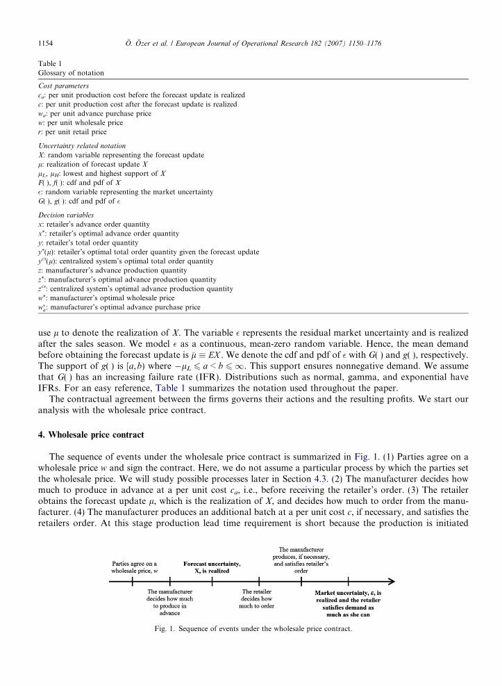
Table 1Glossary of notation

Cost parameters

ca: per unit production cost before the forecast update is realizedc: per unit production cost after the forecast update is realizedwa: per unit advance purchase pricew: per unit wholesale pricer: per unit retail price

Uncertainty related notation

X: random variable representing the forecast updatel: realization of forecast update X

lL, lH: lowest and highest support of X

F(Æ), f(Æ): cdf and pdf of X

�: random variable representing the market uncertaintyG(Æ), g(Æ): cdf and pdf of �

Decision variables

x: retailer’s advance order quantityx*: retailer’s optimal advance order quantityy: retailer’s total order quantityy*(l): retailer’s optimal total order quantity given the forecast updateycs(l): centralized system’s optimal total order quantityz: manufacturer’s advance production quantityz*: manufacturer’s optimal advance production quantityzcs: centralized system’s optimal advance production quantityw*: manufacturer’s optimal wholesale pricew�a: manufacturer’s optimal advance purchase price


use l to denote the realization of X. The variable � represents the residual market uncertainty and is realizedafter the sales season. We model � as a continuous, mean-zero random variable. Hence, the mean demandbefore obtaining the forecast update is �l � EX . We denote the cdf and pdf of � with G(Æ) and g(Æ), respectively.The support of g(Æ) is [a,b) where �lL 6 a < b 61. This support ensures nonnegative demand. We assumethat G(Æ) has an increasing failure rate (IFR). Distributions such as normal, gamma, and exponential haveIFRs. For an easy reference, Table 1 summarizes the notation used throughout the paper.

The contractual agreement between the firms governs their actions and the resulting profits. We start ouranalysis with the wholesale price contract.

4. Wholesale price contract

The sequence of events under the wholesale price contract is summarized in Fig. 1. (1) Parties agree on awholesale price w and sign the contract. Here, we do not assume a particular process by which the parties setthe wholesale price. We will study possible processes later in Section 4.3. (2) The manufacturer decides howmuch to produce in advance at a per unit cost ca, i.e., before receiving the retailer’s order. (3) The retailerobtains the forecast update l, which is the realization of X, and decides how much to order from the manu-facturer. (4) The manufacturer produces an additional batch at a per unit cost c, if necessary, and satisfies theretailers order. At this stage production lead time requirement is short because the production is initiated

Fig. 1. Sequence of events under the wholesale price contract.


closer to the sales season. Hence, the manufacturer per unit production cost is higher than his cost in the ear-lier production stage; i.e., ca < c. Finally, (5) market uncertainty � is realized and the retailer satisfies demandfrom on-hand inventory at a fixed price r. We assume that w 2 [c, r]; otherwise it is never profitable for themanufacturer to produce or the retailer to place any order.

Note that three decisions are made in a sequel: the wholesale price, the manufacturer’s advance productionquantity and the retailer’s order quantity. We characterize the optimal decisions by using a backward induc-tion algorithm; i.e., solve for the last decision first. The manufacturer’s production decision does not affect theretailer’s ordering policy. Hence, the retailer’s order decision depends only on the wholesale price. Therefore,first we solve the retailer’s ordering decision for a given wholesale price. The manufacturer’s advance produc-tion decision depends closely on the retailer’s order decision and the wholesale price. Hence, next we solve themanufacturer’s production problem. The pricing decision affects all other decisions. Therefore, we solve forthe optimal wholesale price last.

4.1. The retailer’s problem

Given an order quantity y and the forecast update l, the retailer’s expected profit is

Prðy; lÞ ¼ rE�½minðy; lþ �Þ� � wy: ð1Þ
The retailer maximizes this newsvendor problem and determines her optimal order quantity
y�ðlÞ � lþ G�1 r � wr

� �: ð2Þ

4.2. The manufacturer’s problem

The manufacturer can save from production cost by initiating part of his production before the forecastupdate. At the time of the advance production decision, however, the retailer’s total order is unknown. Hence,the manufacturer trades off between excess inventory and lower production cost. Let z P 0 units be the man-ufacturer’s advance production quantity. Since the retailer orders only after the forecast update, the manufac-turer builds all z units to stock. Given the advance production quantity and the retailer’s optimal orderquantity, manufacturer’s expected profit under a wholesale price contract is

Pmðw; zÞ � wEX y�ðX Þ � caz� cEX ðy�ðX Þ � zÞþ: ð3Þ
Next we characterize the manufacturer’s advance production policy. We defer all the proofs and some of thetechnical lemmas to Appendix A.
Theorem 1

1. The manufacturer optimally produces z� ¼ F �1 c�cac

� �þ G�1 r�w

r

� �units in advance.

2. z* is decreasing in ca and z* 2 (y*(lL), y*(lH)).

This theorem characterizes the manufacturer’s advance production policy. Part 1 characterizes the optimaladvance production quantity. From Eq. (2), the manufacturer knows that the retailer will order at least y*(lL)units. Part 2 shows that the optimal production quantity is increasing in the cost saving from advance produc-tion. When the advance production cost is lower than c, the manufacturer optimally produces more than theminimum possible retailer order. Hence, he faces excess inventory risk. In particular, when ca < c, the manu-facturer optimally stocks more than y*(lL).

4.3. Contract pricing decision

So far we have characterized the retailer’s optimal order size and the manufacturer’s optimal advance pro-duction quantity for a given wholesale price w. This scenario is possible when the product is a commodity andthe firms take the wholesale price as given. Next, we study the scenario in which the manufacturer sets the


wholesale price as a Stackelberg leader. The retailer responds by setting her order size. This scenario is pos-sible, for example, when the manufacturer builds a custom product and is the only producer of this product.

To solve for the manufacturer’s optimal wholesale price, we substitute the optimal advance productionquantity z* characterized in Theorem 1 Part 1 to Eq. (3) and solve for

3 We

w� � arg maxw

Pmðw; z�Þ:

The next theorem characterizes the manufacturer’s optimal wholesale price.

Theorem 2

1. The manufacturer’s expected profit in Eq. (3) is unimodal in w. Hence, the manufacturer’s optimal wholesale

price is

w� ¼ rð1� Gðv�ÞÞ; where v�is the solution to

rð1� GðvÞÞ 1� gðvÞð�lþ vÞ1� GðvÞ

� �� ca ¼ 0:

2. w* is increasing3 in �l.

3. w* is increasing in ca.

Part 1 characterizes the manufacturer’s optimal wholesale price. Part 2 shows that the manufacturer’s opti-mal wholesale price is higher when expected demand is high. Part 3 reveals that reducing the advance produc-tion cost enables the manufacturer to reduce his optimal wholesale price. These results show that themanufacturer would be charging a higher wholesale price when the market potential for the product is highand when it is costly to produce the product. The manufacturer, for example, can use a new technology or aprocess such as quick response initiatives to reduce the cost of production. The above theorem shows that thebenefit of such improvements would be shared with the retailer through reduced wholesale prices.

5. Dual purchase contract

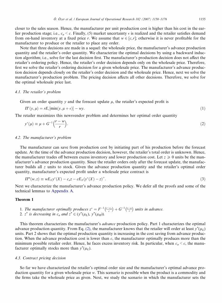
This contract specifies two prices, an advance purchase price wa and the regular wholesale price w. Theretailer pays wa for each unit that she orders before observing the forecast update and w after the forecastupdate. The sequence of events under the dual purchase contract is summarized in Fig. 2. (1) Parties agreeon w and wa. Here, we do not assume a particular process by which contract parameters are set. Later, in Sec-tion 5.3, we address how the contract terms are set. (2) The retailer decides how much to order in advance ofobtaining the forecast update and pays wa per unit of advance order. (3) The manufacturer decides how muchto produce in advance at a per unit production cost ca. (4) The retailer obtains the forecast update l and deci-des how much more to order and pays w per unit. (5) The manufacturer produces an additional batch at a perunit price c, if necessary, and satisfies the retailer’s total order. (6) Market uncertainty � is realized and theretailer satisfies demand from on-hand inventory as much as possible at a per unit price r.

Note that under this contract four decisions are made in a sequel: the dual purchase contract prices, theretailer’s advance purchase quantity, the manufacturer’s advance production quantity, and the retailer’s reg-ular order quantity. We solve for the optimal decisions by using a backward induction algorithm. The man-ufacturer’s production decision does not affect the retailer’s order quantity. Hence, first we solve for theretailer’s problem. The manufacturer’s advance production decision depends closely on the retailer’s orderdecision. Hence, second we solve the manufacturer’s problem. The pricing decision affects all other decisions.Hence, we solve for the contract-pricing problem last.

use the terms ‘‘increasing’’ and ‘‘decreasing’’ in the strong sense; i.e., increasing means strictly increasing.

Fig. 2. Sequence of events under the dual purchase contract.


5.1. The retailer’s problem

Given a dual purchase contract, the retailer has two opportunities to place orders: before and after the fore-cast update. While the retailer saves on procurement cost by placing an advance order, she obtains betterinformation by placing an order after the forecast update. Thus, the retailer faces a tradeoff between lowercost and better information. Let x be the retailer’s order quantity before the forecast update and y be the retai-ler’s total order quantity after the forecast update. To maximize her profit, the retailer solves the followingdynamic optimization problem:

maxxP0

PrðxÞ ¼ EX prðx;X Þ � wax; ð4Þ

where prðx; lÞ ¼ maxyPx

rE�½minðy; lþ �Þ� � wðy � xÞ: ð5Þ

When wa > w, the optimal advance purchase quantity is zero because the retailer can purchase at a cheaperprice after obtaining the forecast update. This case is equivalent to the wholesale price contract. Hence, in thissection we consider wa 6 w. The following theorem summarizes the retailer’s optimal policy.

Theorem 3

1. The solution to Eq. (5) is max(y*(l),x), where y�ðlÞ � lþ G�1 r�wr

� �, and it is decreasing in w.

2. Pr(x) is concave in x and limjxj!1Pr(x) = �1. Hence, the objective function in Eq. (4) has a maximizer x*,which is the retailer’s optimal advance purchase quantity.

This theorem shows that the retailer’s optimal order policy is an order-up-to policy. Before observing theforecast update, the retailer orders up to x* units. After the forecast update, if x* 6 y*(l), she orders up toy*(l). Therefore, the retailer’s additional order quantity after the forecast update is (y*(l) � x*)+. Notice thatorder-up-to level y*(l) is the same as the optimal order quantity under the wholesale price contract given inEq. (2). Hence, when the manufacturer offers a dual purchase contract, the retailer orders at least as much aswhat she would order under a wholesale price contract. This result implies that the dual purchase contract is amechanism that induces the retailer to place additional orders. Next we further characterize the retailer’sadvance purchase quantity.

Theorem 4

1. When wa 2 [ca,s(w)] where sðwÞ � r 1�R lH

lLGðy�ðlH Þ � lÞf ðlÞdl

h i< w, the retailer orders only before

the forecast update. In this case, x* is the solution to the first order condition:

r½1�Z lH

lL

Gðx� lÞf ðlÞdl� � wa ¼ 0: ð6Þ

x* is decreasing in wa and x* P y*(lH). When wa = s(w), we have x* = y*(lH).

2. When wa 2 (s(w),w), the optimal advance purchase quantity x* is the solution to the following first order

condition:


w 1� F x� G�1 r � wr

� �� þ r

Z x�G�1 r�wrð Þ

lL

ð1� Gðx� lÞÞf ðlÞdl

" #� wa ¼ 0: ð7Þ

x* is decreasing in wa, increasing in w and x* 2 (y*(lL),y*(lH)).
3. When wa = w, x* can take any value between [0,y*(lL)]. The retailer’s total purchase quantity and her
expected profit under the dual purchase contract and under the wholesale price contract are equal. Hence,

without loss of generality, x* = 0.

4. x* > y*(lL) if and only if wa < w.

Part 1 shows that when the advance purchase price wa is below the threshold s(w), the advance purchasequantity is larger than y*(lH). This result, together with Theorem 3 Part 1, implies the following. The retailerorders only before observing the forecast update. Intuitively, the discount is deep enough to offset the retailer’sgain from waiting and observing the forecast update before placing his order. Part 2 shows that when theadvance purchase price wa 2 (s(w), w), the optimal advance purchase quantity x* 2 (y*(lL),y*(lH)). Thus,given a discount, the retailer orders more than y*(lL) units in advance and exactly (y*(l) � x*)+ units afterobserving the forecast update. A higher wholesale price induces a larger advance purchase quantity. Part 3shows that when wa = w, the retailer orders nothing in advance. Part 4 states that a discount induces anadvance purchase of x* > y*(lL).

5.2. The manufacturer’s problem

Given the retailer’s optimal response as characterized by Theorems 3 and 4, the retailer places part of herorder before the forecast update. Hence, the manufacturer’s expected profit under a dual purchase contractcan be written as

PmdpðzÞ ¼

wax� � caz� cðx� � zÞþ; wa 2 ½ca; sðwÞ�;wax� þ wEX ðy�ðX Þ � x�Þþ � caz� cEX ðmaxfx�; y�ðX Þg � zÞþ; wa 2 ðsðwÞ;w�:

(ð8Þ

To decide on the advance production quantity, the manufacturer solves

maxzP0

PmdpðzÞ:

Next we characterize the advance production quantity z�dp.

Theorem 5

1. The profit function PmdpðzÞ is strictly concave in z.

2. When wa 2 [ca,s(w)], the optimal advance production quantity is z�dp ¼ x�. When wa 2 (s(w), w], we havez�dp ¼ max x�; F �1 c�ca

c

� �þ G�1 r�w

r

� �� . For all wa, we have z�dp P F �1 c�ca

c

� �þ G�1 r�w

r

� �.

This theorem fully characterizes the manufacturer’s production policy. Part 2 shows that the manufac-turer’s optimal advance production is at least as much as the retailer’s advance order quantity. This makesintuitive sense because the manufacturer’s advance production cost is ca < c. Part 2 also characterizes the man-ufacturer’s minimum advance production quantity; i.e., he optimally produces at least F �1 c�ca

c

� �þ G�1 r�w

r

� �units in advance.

5.3. Contract pricing decision

Here we solve for the optimal contract parameters wa and w. We consider two possible scenarios. In the firstscenario, the manufacturer and the retailer take the wholesale price w as given. However, the manufacturerdecides whether to offer the advance purchase price wa. If he does, he maximizes his profit by deciding onwa. In most supply chains, the firms establish a relationship, hence a supply chain, for the product by agreeing


on a wholesale price long before the actual production is initiated or any forecast update is obtained. Thisprice could also be set by the market. Neither the manufacturer nor the retailer may be able to enforce thewholesale price that maximizes their own profit. However, the manufacturer can offer an advance purchaseprice on his own discretion. In the second scenario, the manufacturer as the Stackelberg leader sets bothwa and w.

To obtain the optimal advance purchase price, the manufacturer solves the following problem:

w�a � argmaxwa2½ca;w�Pmdpðwa; z�dpÞ; ð9Þ

where Pmdp is defined in Eq. (8). Next we characterize the solution.

Theorem 6. Let w‘ � r(1 � G(v‘)) where v‘ satisfies rð1� Gðv‘ÞÞ 1� gðv‘ÞðlLþv‘Þ1�Gðv‘Þ

h i¼ 0.

1. When w 6 w‘, the optimal advance purchase price is w�a ¼ w.

2. When w > w‘, the optimal advance purchase price is w�a < w.

The first part states that if the wholesale price is low; i.e., w < w‘, then the manufacturer should not offer anadvance purchase discount and hence revert back to the wholesale price contract (simply by setting wa = w). Inthis case, the retailer has no incentive to order in advance (recall from Theorem 4 Part 3). However, when thewholesale price is larger than the threshold w‘, it is optimal for the manufacturer to provide a discount fororders placed prior to the forecast update.

Theorem 7. The dual purchase contract with ðw�a;wÞ increases the manufacturer’s profit over the wholesale price

contract if and only if w > w‘.

The retailer always has the option not to place any order before the forecast update. Therefore, the retaileris always better off with a dual purchase contract over a wholesale price contract when wa < w. Hence, thistheorem states that the manufacturer can strictly improve his expected profit as well as the retailer’s expectedprofit when he sets and offers the advance purchase price.

Now consider the scenario in which the manufacturer sets both wa and w. To do so, he solves

P�dp � maxwa;w½Pm

dpðwa;w; z�dpÞ�; ð10Þ

where Pmdpðwa;w; z�dpÞ is as defined in Eq. (8). We have the following result.

Theorem 8. When the manufacturer sets the wholesale price, the optimal dual purchase contract always increases

his profit over the optimal wholesale price contract.

Hence, the manufacturer always prefers the dual purchase contract when he sets both prices. Whether thedual purchase contract also improves retailer’s profit over the wholesale price contract is not analytically con-clusive when the manufacturer sets both prices. However, in most of our numerical experiments in Section 9,the retailer’s profit was also higher under dual purchase contract.

In brief, Theorem 7 states that when the manufacturer sets the advance purchase price, the dual purchasecontract improves both the manufacturer’s and the retailer’s profits over the wholesale price contract, henceenabling strict Pareto improvement. Theorem 8 states that when the manufacturer sets the advance purchaseprice and the wholesale price, the dual purchase contract always improves the manufacturer’s profit over theoptimal wholesale price contract.

6. Supply chain efficiency

This section provides the reason why the manufacturer can achieve higher profits with the dual purchasecontract. To do so, we consider the centralized supply chain, for which no internal payment needs to beexchanged. In particular, we compare the resulting optimal profit of the centralized supply chain with the totalsupply chain profit of the decentralized system; i.e., the sum of the manufacturer’s and the retailer’s optimal


expected profits. When the centralized supply chain profit and decentralized total profit are equal, we say thesystem is coordinated. The difference in profits is a measure of decentralized supply chain’s efficiency.

The centralized system determines first the advance production quantity and the additional productionquantity after obtaining the forecast update. Let z be the centralized system’s advance production quantityand y be the total production quantity after the forecast update. The centralized system solves the followingdynamic program:

maxzP0

PcsðzÞ ¼ EX pcsðz;X Þ � caz; ð11Þ

where pcsðz;lÞ ¼ maxyPz

rE�½minðy; lþ �Þ� � cðy � zÞ: ð12Þ

The following theorem characterizes the centralized system’s production policy.

Theorem 9

1. The solution to (12) is max(z,ycs(l)) where ycsðlÞ ¼ lþ G�1 r�cr

� �for all l 2 [lL,lH].

2. Pcs(z) is concave in z and limjzj!1Pcs(z) = �1. Hence, the objective function in Eq. (11) has a maximizer

zcs, which is the centralized system’s optimal advance production quantity.

This theorem characterizes the centralized system’s production policy to be a produce-up-to policy. The cen-tralized system produces zcs before the forecast update. After the forecast update, if zcs

6 ycs(l), the centralizedsystem produces up to ycs(l). Next we characterize zcs.

Theorem 10

1. When ca 2 [0,scs(c)] where scsðcÞ � r 1�R lH

lLGðycsðlH Þ � lÞf ðlÞdl

h i< c, the centralized system produces

only before the forecast update. In this case, zcs is the solution to the first order condition:

r 1�Z lH

lL

Gðz� lÞf ðlÞdl

�� ca ¼ 0: ð13Þ

zcs is decreasing in ca and zcs P ycs(lH). When ca = scs(c), we have zcs = ycs(lH).

2. When ca 2 (scs(c), c), optimal advance production quantity zcs is the solution to the following first order

condition:

c 1� F z� G�1 r � cr

� �� þ r

Z z�G�1ðr�cr Þ

lL

ð1� Gðz� lÞÞf ðlÞdl

" #� ca ¼ 0: ð14Þ

zcs is decreasing in ca, increasing in c and zcs 2 (ycs(lL),ycs(lH)).

3. When ca = c, zcs can take any value between [0,ycs(lL)]. Hence, without loss of generality, zcs = 0.

4. zcs > ycs(lL) if and only if ca < c.5. zcs > F �1 c�ca

c

� �þ G�1 r�w

r

� �for all ca < c.

The advance production and the total production quantity determine supply chain profit. Therefore, toachieve channel coordination in a decentralized system, the advance production quantity must be equal tozcs and the total production quantity must be equal to max(zcs,ycs(l)) for all l 2 [lL,lH].

First consider the wholesale price contract. It is well known that the wholesale price contract does not coor-dinate even the supply chain without a forecast update, resulting in supply chain inefficiency (Pasternack,1985). This contract also does not coordinate the supply chain discussed here. To observe this, note thatthe manufacturer’s advance production quantity under this contract is less than the centralized system’sadvance production quantity (compare Theorem 1 Part 1 with Theorem 10 Part 5). Next consider the dualpurchase contract. Can a dual purchase contract coordinate, if not, improve the efficiency of the supply chain?

Theorem 11. There always exists a dual purchase contract under which supply chain profit is greater than the

profit under a given wholesale price contract. In other words, for any w, there exists wa such that


EX Prðy�ðX Þ;X Þ þPmðw; z�Þ < Prðx�Þ þPmdpðz�dpÞ, where each profit function is defined in (1), (3),(4), and (8),

respectively.

This result shows that a dual purchase contract mitigates the inefficiency caused by a wholesale price con-tract. The wholesale price contract causes double marginalization when w > c (Pasternack, 1985). The dualpurchase contract mitigates the adverse effect of double marginalization by providing an additional opportu-nity to order at a discounted advance purchase price wa < w. Therefore, by offering an advance purchase pricethe manufacturer can increase the supply chain efficiency, retain part of the savings and leave the remaining tothe retailer.

7. Without advance production

Next we investigate whether the strict Pareto improvement over the wholesale price contract is due to theadvance production capability. In other words, can the manufacturer and the retailer be better off with a dualpurchase contract than with a wholesale price contract even when ca > c? To answer this question, first notethat when ca > c, the optimal advance production amount is zero under both contracts because the manufac-turer can produce at a cheaper cost after obtaining retailer’s total order. Hence, the manufacturer produces infull after the retailer places her order. Note that the retailer’s order policy remains the same as before. Shefollows the optimal ordering policy characterized in the previous sections for both contracts. Hence, the onlydecision we need to analyze is the manufacturer’s pricing decision. We start with the wholesale price contract.

The manufacturer’s expected profit under the wholesale price contract can be written as

PmðwÞ ¼ ðw� cÞEX y�ðX Þ: ð15Þ
The next theorem characterizes the manufacturer’s optimal.
Theorem 12

1. The manufacturer’s profit in Eq. (15) is unimodal in w. Hence, if he can, the manufacturer sets the wholesale

price to

w� ¼ rð1� Gðv�ÞÞ;where v�is the solution to

rð1� GðvÞÞ 1� gðvÞð�lþ vÞ1� GðvÞ

� �� c ¼ 0:

We denote the solutions of the above equations with w�L and v�L when the probability of facing the worst pos-sible forecast realization is one (Prob{X = lL} = 1), and hence �l ¼ lL.

2. w* is increasing in �l and w� P w�L.

3. w* is increasing in c.

From Part 1, if the manufacturer knows with certainty that the retailer will face the worst possible salesseason; i.e., if X = lL with probability one, then he optimally sets the wholesale price equal to w�L. This whole-sale price is the lowest price that the manufacturer would offer. Part 2 shows that the manufacturer optimallyoffers a higher wholesale price when the forecast update is expected to be high. Part 3 shows that the manu-facturer optimally chooses a higher wholesale price if his regular production cost increases.

Without advance production, the manufacturer’s expected profit under the dual purchase contract simpli-fies to the following:

PmdpðwaÞ ¼

ðwa � cÞx�; wa 2 ½c; sðwÞ�;ðwa � cÞx� þ ðw� cÞEX ðy�ðX Þ � x�Þþ; wa 2 ðsðwÞ;w�:

�ð16Þ

Theorem 13. When ca > c, the dual purchase contract with w�a increases the manufacturer’s profit over the

wholesale price contract if and only if w > w�L.

This theorem shows that strict Pareto improvement under the dual purchase contract is achievable even fora manufacturer that does not have advance production capability. In particular, if the manufacturer can set


the advance purchase price, he can create a strict Pareto improvement over any wholesale price contract byoffering the advance purchase price as long as w > w�L. The strict Pareto improvement in this case is alsodue to having two order opportunities. The discounted advance purchase price reduces the adverse affect ofdouble marginalization.

8. Manufacturer’s risk attitude

So far, we have shown how a dual purchase contract increases expected profits. Our next aim is to charac-terize how the dual purchase contract also reduces the manufacturer’s profit volatility and how it affects a riskaverse manufacturer.

Under a wholesale price contract, the manufacturer’s profit is uncertain prior to the forecast update. Thisuncertainty in profit projection often discourages capital investment. The manufacturer can, however, reducethis uncertainty by using a dual purchase contract.

Theorem 14. Under a dual purchase contract where ca > c, the variance of the manufacturer’s profit is

Vardp(wa) � (w � c)2Var(y*(X) � x*)+, which is less than or equal to the variance of the manufacturer’s profit

under the wholesale price contract. This variance equals zero when wa 2 [c,s(w)] and it is increasing in wa whenwa 2 (s(w), w].

Note that the variance depends on wa through the retailer’s optimal advance purchase quantity x*. A dualpurchase contract reduces the manufacturer’s profit volatility and, hence, enables risk hedging. If a manufac-turer is risk averse, then he can determine the optimal advance purchase price by trading off expected profitand profit variance. The mean-variance tradeoff is widely used in portfolio theory and can be reconciled withthe expected utility approach by using a quadratic utility function. Consider utility function uðxÞ ¼ ax� 1

2bx2

(a > 0,b P 0,x 6 a/b). When x is random, let �x � EðxÞ. The expected utility is E½uðxÞ� ¼ a�x� 12b�x2 � 1

2bVarðxÞ.

Clearly, for all feasible x’s with the same expected value, the optimal one must have minimum variance. Alter-natively, note that maximizing expected utility is equivalent to maximizing the certainty equivalent, which canbe approximated as c � �xþ 1

2u00ð�xÞu0ð�xÞ VarðxÞ (Luenberger, 1998, p. 256). For utility functions with constant abso-

lute risk aversion k, we have u00ð�xÞu0ð�xÞ ¼ �k.

Specifically, the manufacturer solves the following optimization problem:

maxwa

PmraðwaÞ � Pm

dpðwaÞ � kVardpðwaÞ: ð17Þ

Note that, given the retailer’s response, the manufacturer’s objective function is

PmraðwaÞ ¼

ðwa � cÞx�; wa 2 ½c; sðwÞ�;ðwa � cÞx� þ ðw� cÞEX ðy�ðX Þ � x�Þþ � kðw� cÞ2VarX ðy�ðX Þ � x�Þþ; wa 2 ðsðwÞ;w�:

(

ð18Þ
The coefficient k reflects the manufacturer’s risk attitude. When k = 0, the manufacturer is risk neutral as in
the previous section. When k > 0, the manufacturer is risk averse and a larger k implies that the manufactureris more risk averse. When k < 0, the manufacturer is risk seeking.

Theorem 15. Let k � � w�c�ry�ðlLÞgðy�ðlLÞ�lLÞ2ðw�cÞ2ð�l�lLÞ

.

1. When k > k, the manufacturer prefers the dual purchase contract with ðw�a;wÞ to a wholesale price contract

with w. The optimal advance purchase price w�a is decreasing in k.

2. When k 6 k, the manufacturer prefers the wholesale price contract with w to a dual purchase contract with

(wa,w).

The theorem states that when the manufacturer’s risk aversion factor is above the threshold k, he always

prefers a dual purchase contract. The theorem also characterizes the risk aversion threshold above whichany manufacturer would prefer the dual purchase contract over the wholesale price contract. Furthermore,


to increase the advance purchase quantity and hence reduce his profit volatility, a manufacturer with higherrisk aversion offers a greater discount.

9. Numerical examples

The purpose of this section is to illustrate some of our results and numerically compare the profits under thedual purchase contract to the profits under the wholesale price contract. Our base case is ca = 2.5, c = 3 andr = 10. The forecast update X follows the truncated normal distribution on [8, 24] with mean 16 and standarddeviation rX. The market uncertainty � also follows the truncated normal distribution on [�8,8] with mean 0and standard deviation r�. The truncated normal distribution has IFR.

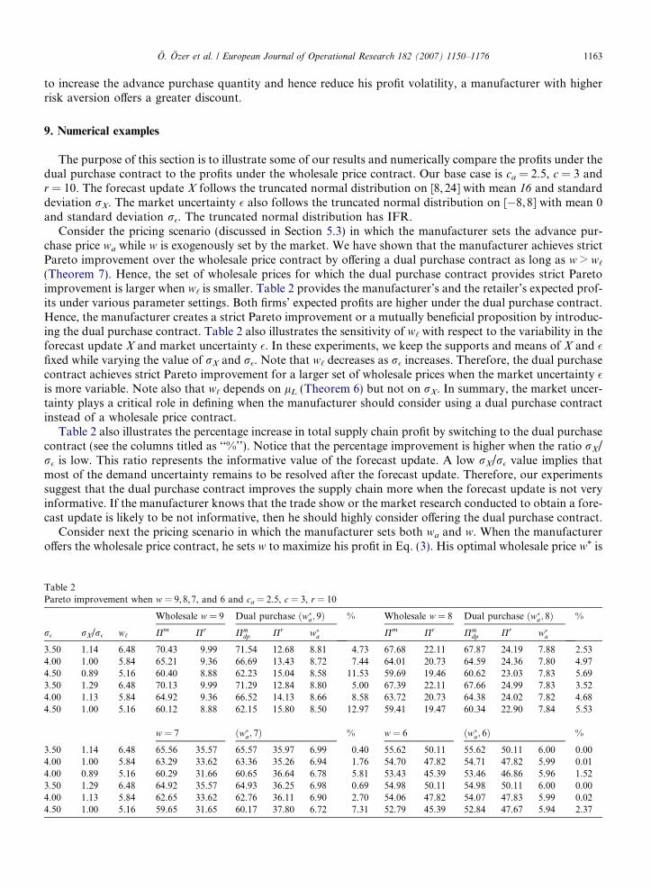
Consider the pricing scenario (discussed in Section 5.3) in which the manufacturer sets the advance pur-chase price wa while w is exogenously set by the market. We have shown that the manufacturer achieves strictPareto improvement over the wholesale price contract by offering a dual purchase contract as long as w > w‘

(Theorem 7). Hence, the set of wholesale prices for which the dual purchase contract provides strict Paretoimprovement is larger when w‘ is smaller. Table 2 provides the manufacturer’s and the retailer’s expected prof-its under various parameter settings. Both firms’ expected profits are higher under the dual purchase contract.Hence, the manufacturer creates a strict Pareto improvement or a mutually beneficial proposition by introduc-ing the dual purchase contract. Table 2 also illustrates the sensitivity of w‘ with respect to the variability in theforecast update X and market uncertainty �. In these experiments, we keep the supports and means of X and �fixed while varying the value of rX and r�. Note that w‘ decreases as r� increases. Therefore, the dual purchasecontract achieves strict Pareto improvement for a larger set of wholesale prices when the market uncertainty �is more variable. Note also that w‘ depends on lL (Theorem 6) but not on rX. In summary, the market uncer-tainty plays a critical role in defining when the manufacturer should consider using a dual purchase contractinstead of a wholesale price contract.

Table 2 also illustrates the percentage increase in total supply chain profit by switching to the dual purchasecontract (see the columns titled as ‘‘%’’). Notice that the percentage improvement is higher when the ratio rX/r� is low. This ratio represents the informative value of the forecast update. A low rX/r� value implies thatmost of the demand uncertainty remains to be resolved after the forecast update. Therefore, our experimentssuggest that the dual purchase contract improves the supply chain more when the forecast update is not veryinformative. If the manufacturer knows that the trade show or the market research conducted to obtain a fore-cast update is likely to be not informative, then he should highly consider offering the dual purchase contract.

Consider next the pricing scenario in which the manufacturer sets both wa and w. When the manufactureroffers the wholesale price contract, he sets w to maximize his profit in Eq. (3). His optimal wholesale price w* is

Table 2Pareto improvement when w = 9,8,7, and 6 and ca = 2.5, c = 3, r = 10

Wholesale w = 9 Dual purchase ðw�a; 9Þ % Wholesale w = 8 Dual purchase ðw�a; 8Þ %

r� rX/r� w‘ Pm Pr Pmdp Pr w�a Pm Pr Pm

dp Pr w�a

3.50 1.14 6.48 70.43 9.99 71.54 12.68 8.81 4.73 67.68 22.11 67.87 24.19 7.88 2.534.00 1.00 5.84 65.21 9.36 66.69 13.43 8.72 7.44 64.01 20.73 64.59 24.36 7.80 4.974.50 0.89 5.16 60.40 8.88 62.23 15.04 8.58 11.53 59.69 19.46 60.62 23.03 7.83 5.693.50 1.29 6.48 70.13 9.99 71.29 12.84 8.80 5.00 67.39 22.11 67.66 24.99 7.83 3.524.00 1.13 5.84 64.92 9.36 66.52 14.13 8.66 8.58 63.72 20.73 64.38 24.02 7.82 4.684.50 1.00 5.16 60.12 8.88 62.15 15.80 8.50 12.97 59.41 19.47 60.34 22.90 7.84 5.53

w = 7 ðw�a; 7Þ % w = 6 ðw�a; 6Þ %

3.50 1.14 6.48 65.56 35.57 65.57 35.97 6.99 0.40 55.62 50.11 55.62 50.11 6.00 0.004.00 1.00 5.84 63.29 33.62 63.36 35.26 6.94 1.76 54.70 47.82 54.71 47.82 5.99 0.014.00 0.89 5.16 60.29 31.66 60.65 36.64 6.78 5.81 53.43 45.39 53.46 46.86 5.96 1.523.50 1.29 6.48 64.92 35.57 64.93 36.25 6.98 0.69 54.98 50.11 54.98 50.11 6.00 0.004.00 1.13 5.84 62.65 33.62 62.76 36.11 6.90 2.70 54.06 47.82 54.07 47.83 5.99 0.024.50 1.00 5.16 59.65 31.65 60.17 37.80 6.72 7.31 52.79 45.39 52.84 47.67 5.94 2.37

Table 3Pareto improvement when manufacturer sets w

rX r� rX/r� Wholesale Dual purchase %

Pm Pr w* Pmdp Pr (wa,w)*

ca = 2, c = 3, r = 64.00 3.50 1.14 33.86 5.77 5.42 35.30 7.65 (5.29, 5.62) 8.384.00 4.00 1.00 31.14 6.04 5.36 33.03 7.73 (5.28, 5.58) 9.634.00 4.50 0.89 28.62 5.14 5.42 31.02 6.28 (5.40, 5.72) 10.494.50 3.50 1.29 33.22 5.77 5.42 34.94 7.72 (5.27, 5.62) 9.414.50 4.00 1.13 30.50 6.04 5.36 32.69 7.79 (5.26, 5.58) 10.784.50 4.50 1.00 27.98 5.14 5.42 30.69 6.31 (5.38, 5.72) 11.71

ca = 2.5, c = 3, r = 64.00 3.50 1.14 29.89 4.67 5.52 30.73 5.35 (5.48, 5.58) 4.404.00 4.00 1.00 27.49 4.79 5.48 28.44 5.55 (5.45, 5.54) 5.304.00 4.50 0.89 25.49 3.07 5.64 26.64 3.87 (5.61, 5.82) 6.834.50 3.50 1.29 29.60 4.67 5.52 30.42 5.41 (5.48, 5.56) 4.554.50 4.00 1.13 27.20 4.79 5.48 28.10 5.54 (5.45, 5.56) 5.164.50 4.50 1.00 25.20 3.07 5.64 26.40 3.86 (5.60, 5.88) 7.04

ca = 2, c = 3, r = 104.00 3.50 1.14 74.73 12.52 8.78 76.17 15.89 (8.56, 9.16) 5.514.00 4.00 1.00 69.51 13.93 8.58 71.71 17.19 (8.43, 8.98) 6.544.00 4.50 0.89 64.26 14.18 8.48 67.23 17.00 (8.43, 8.98) 7.384.50 3.50 1.29 74.09 12.52 8.78 75.97 15.72 (8.54, 9.18) 5.874.50 4.00 1.13 68.87 13.93 8.58 71.52 17.03 (8.42, 9.00) 6.944.50 4.50 1.00 63.62 14.18 8.48 67.05 16.82 (8.42, 9.00) 7.80

ca = 2.5, c = 3, r = 104.00 3.50 1.14 70.50 11.36 8.88 71.54 12.70 (8.81, 9.00) 2.914.00 4.00 1.00 65.51 12.37 8.72 66.73 14.20 (8.65, 8.88) 3.924.00 4.50 0.89 60.61 12.09 8.68 62.27 14.42 (8.64, 9.12) 5.494.50 3.50 1.29 70.20 11.36 8.88 71.29 12.86 (8.80, 9.00) 3.184.50 4.00 1.13 65.22 12.37 8.72 66.53 14.62 (8.62, 8.94) 4.594.50 4.50 1.00 60.31 12.09 8.68 62.22 14.38 (8.63, 9.24) 5.80


characterized in Theorem 2 Part 1. When he offers the dual purchase contract, he sets both wa and w to max-imize his profit. He solves the optimization problem in Eq. (10). In Table 3, we compare the profits resultingfrom the manufacturer’s optimal choices. As Theorem 8 proves, the manufacturer’s profit is always higherunder the dual purchase contract. In all the experiments, the retailer’s profit is also higher under the dual pur-chase contract. The percentage improvement in supply chain profit tends to increase when rX/r� is low. Com-paring the ca = 2.5, c = 3 and the ca = 2, c = 3 cases, we note that the percentage improvement is higher whenthe cost difference between the advance production and normal production is high. Intuitively, the dual pur-chase contract allows the supply chain to enjoy low production costs by providing the retailer incentive toplace most of her need through advance orders.

10. Conclusion

We study a supply chain in which the retailer observes a forecast update and the manufacturer produces tosatisfy the retailer’s order. Under a wholesale price contract, the retailer places orders only after observing theforecast update. Preserving the simplicity, we study another price-only contract, the dual purchase contract,which provides the retailer with incentive and flexibility to order both before and after the forecast update. Weshow that the dual purchase contract increases supply chain profit as well as the retailer’s profit, and identifyconditions under which it also increases the manufacturer’s profit and hence creates a strict Pareto improve-ment. The analytical results together with the numerical examples suggest that the dual purchase contract is


likely to achieve strict Pareto improvement over the wholesale price contract when (1) low cost advance pro-duction is available, (2) the manufacturer is risk averse, (3) the market uncertainty is high, or (4) the worstpossible forecast update value is low.

We have also investigated other supply chain scenarios (Wei, 2003). For example, results similar to those inTheorem 7 are shown when the manufacturer faces excess inventory risk due to an exogenous minimum pro-duction quantity requirement. Manufacturers must often keep labor force utilization at a production facilityabove a certain percentage due to long term labor contracts (see Fisher and Raman, 1996, for examples). Theimposed minimum production quantity generates excess inventory risk similar to the case of advance produc-tion. Theorem 7 continues to hold in this case. Practitioners often characterize the forecast update X with sim-ple distributions such as low and high forecast update with a Bernoulli distribution. For such cases, thethresholds and the decision variables, such as the optimal advance purchase price w�a are characterized inclosed-form solutions.

Price-only contracts are the most prevalent contracts used in practice. Hence, additional research on suchcontracts is needed and will likely to have real impact in practice. There are several fertile avenues for futureresearch. For example, here we studied per unit payments that are independent of the order size. An extensionis to consider a quantity discount scheme. Quantity discounts can induce even larger orders from the retailerfor situations when the forecast realization is low. Note, however, that quantity discount also reduces the man-ufacturer’s profit. Based on the results in this paper, we conjecture that such a contract will also achieve Paretoimprovement over the wholesale price contract. However, the net effect is not quantitatively apparent. Ana-lyzing a dual purchase contract with a quantity discount scheme is an interesting future research question.

Appendix A. Proofs

A.1. Proofs of theorems in Section 4 and required technical lemmas

Proof of Theorem 1. To prove Part 1, we define v � G�1 r�wr

� �and rewrite the manufacturer’s profit in Eq. (3)

as

Pmðw; zÞ ¼ wð�lþ vÞ � caz� cZ lH

z�vðlþ v� zÞf ðlÞdl: ð19Þ

Then, we have dPmðw;zÞdz ¼ �ca þ cð1� F ðz� vÞÞ. Since F(Æ) is increasing on [lL,lH], we conclude that Pm(w,z) is

strictly concave in z on [lL + v,lH + v] and z* is the solution to the first order condition. Hence,z� ¼ F �1 c�ca

c

� �þ v.

Part 2 follows from Part 1 because the forecast update, X, is distributed on [lL,lH]. h

Proof of Theorem 2. First we provide the following lemma as an auxiliary proposition to simplify the proof ofthis theorem.

Lemma 1

Let k(v) be any differentiable function. If

dkðvÞdv¼ a rð1� GðvÞÞ 1� gðvÞðlþ vÞ

1� GðvÞ

� �� cðvÞ

�;

where a > 0; l P 0; r > c(v) P 0; c(v) nondecreasing, then k(v) is unimodal on R.

Proof of Lemma 1. Let �vo be the supremum of the set of points such that gðvÞv1�GðvÞ 6 1. First, we prove that �vo is

finite. Lariviere and Porteus (2001, Lemma 2(c)) proves that �vo is finite when the lowest possible support for �is a = 0. We use a similar argument as in their proof but consider the case where a can take a finite negativevalue. Let t 2 (0, b) and define the truncated random variable �t on [t,b), whose cdf is GtðvÞ ¼ GðvÞ�GðtÞ

1�GðtÞ for allv 2 [t,b). Note that �t has a finite mean since � has a finite mean (in particular, zero mean). Note also thatthe failure rate of �t is equal to the failure rate of � for all v 2 [t,b). Denote the failure rate of �t with ht(Æ).Assume for a contradiction argument that �vo ¼ 1. Then, htðvÞ 6 1

v for all v 2 [t,b). This implies that �t is


stochastically larger than a random variable g with a failure rate hgðvÞ ¼ 1v for v P t (Ross, 1983). We have

1� GgðvÞ ¼ 1v for all v P t since 1� GgðvÞ ¼ exp½�

R vt hgðvÞdv� (Ross, 1983). Then, g has an infinite mean

implying that �t has an infinite mean, too. This contradicts with the fact that �t has a finite mean. Therefore,�vo must be finite. This result implies that �v, the supremum of the set of points such that gðvÞðlþvÞ

1�GðvÞ 6 1, is also finitebecause l P 0.

The second derivative of k(v) is

d2kðvÞdv2

¼ �argðvÞ 1� gðvÞðlþ vÞ1� GðvÞ

� �� arð1� GðvÞÞ d

dvgðvÞðlþ vÞ

1� GðvÞ

� �� a

dcðvÞdv

:

For v 2 (�1,a), we have dkðvÞdv ¼ r � cðvÞ > 0 and hence k(v) is increasing. Since G(Æ) has IFR, we have

ddv

gðvÞðlþvÞ1�GðvÞ

� �> 0 for all v 2 [a,b). Then for v 2 ½a;�v�, we have d2kðvÞ

dv2 < 0 and hence k(v) is strictly concave. For

v 2 ð�v;1Þ, we have dkðvÞdv < 0 and hence k(v) is decreasing. Therefore, k(v) is unimodal on R and it’s maximizer

lies on ½a;�v�. h

Next we prove the theorem. To prove Part 1, we define v � G�1 r�wr

� �. Then, we have w = r(1 � G(v)). Using

this and substituting z* from Theorem 1 Part 1 into Eq. (3) we rewrite the manufacturer’s profit asZ lH

Pmðv; z�Þ ¼ ðrð1� GðvÞÞ � caÞð�lþ vÞ þ ca�l� cF�1 c�ca

cð Þlf ðlÞdl: ð20Þ

Hence, dPmðv;z�Þdv ¼ rð1� GðvÞÞ 1� gðvÞð�lþvÞ

1�GðvÞ

� �� ca. From Lemma 1, Pm(v,z*) is unimodal in v, and the optimal v

is the solution to the first order condition as stated in the theorem. Since v is monotone in w, the profit functionis also unimodal in w.

To prove Part 2, let Pmðv; z�; lÞ � ðrð1� GðvÞÞ � caÞðlþ vÞ þ cal� cR lH

F�1 c�cacð Þ lf ðlÞdl, and v1 and v2 be

the profit maximizing quantity for l1 < l2, respectively. For any v > 0, we have

oPmðv; z�; l2Þov

¼ rð1� GðvÞÞ 1� gðvÞðl2 þ vÞ1� GðvÞ

� �� ca < rð1� GðvÞÞ 1� gðvÞðl1 þ vÞ

1� GðvÞ

� �� ca

¼ oPmðv; z�; l1Þov

:
Hence, oPmðv;z�;l2Þ
ov v¼v1

< oPmðv;z�l1Þov

v¼v1

¼ 0. Since Pm(v,z*,l2) is unimodal in v, we have v2 < v1, and hence

w*(l2) = r(1 � G(v2)) > r(1 � G(v1)) = w*(l1). Therefore, w* is increasing in �l.

To prove Part 3, let Pmðv; z�; caÞ � ½rð1� GðvÞÞ � ca�ð�lþ vÞ þ ca�l� cR lH

F �1 c�cacð Þ lf ðlÞdl, and v1 and v2 be

the profit maximizing quantity for ca1 < ca2, respectively. We have

oPmðv; z�; ca2Þov

¼ rð1� GðvÞÞ 1� gðvÞð�lþ vÞ1� GðvÞ

� �� ca2 < rð1� GðvÞÞ 1� gðvÞð�lþ vÞ

1� GðvÞ

� �� ca1

¼ oPmðv; z�; ca1Þov

:

Hence oPmðv;z�;ca2Þov

v¼v1

< oPmðv;z�;ca1Þov

v¼v1

¼ 0. Since Pm(v,z*,ca2) is unimodal in v, we have v2 < v1, and hence

w*(ca2) = r(1 � G(v2)) > r(1 � G(v1)) = w*(ca1). Therefore, w* is increasing in ca. h


Proof of Theorem 3. To prove Part 1, note that the objective function in Eq. (5) is concave in y becausemin(y,l + �) is concave and expectation preserves concavity. Therefore, its maximizer is y�ðlÞ ¼ lþ G�1 r�w

r

� �,

which is decreasing in w. The maximizer for the constrained problem is max(y*(l),x).To prove Part 2, note from Part 1 that we have

prðx; lÞ ¼rE½minðy�ðlÞ; lþ �Þ� � wðy�ðlÞ � xÞ; x < y�ðlÞ;rE½minðx; lþ �Þ�; x P y�ðlÞ;

�


which is concave in x. Since expectation preserves concavity and the sum of two concave functions is concave,the objective function in Eq. (4) is also concave in x. We also have limjxj!1Pr(x) = �1. Hence, x*, the max-imizer of the objective function, is finite. h

Proof of Theorem 4. To prove Parts 1 and 2, we define v � G r�wr

� �and rewrite the objective function in Eq. (4)

using Theorem 3 Parts 1 and 2:

PrðxÞ ¼

rE minðy�ðX Þ;X þ �Þ � wEðy�ðX Þ � xÞ � wax; x < y�ðlLÞ;R x�vlL

rE minðx; lþ �Þf ðlÞdlþR lH

x�v½rE minðy�ðlÞ; lþ �Þ

�wðy�ðlÞ � xÞ�f ðlÞdl� wax; x 2 ½y�ðlLÞ; y�ðlH Þ�

rE minðx;X þ �Þ � wax; x > y�ðlH Þ:

8>>>>><>>>>>:

To prove Part 1, we first show that s(w) < w. Note that, sðwÞ ¼ r½1�R lH

lLGðlH þ v� lÞf ðlÞdl� <

r½1�R lH

lL

r�wr f ðlÞdl� ¼ w because GðlH þ v� lÞ > GðvÞ ¼ r�w

r for all l 2 [lL,lH).Next for wa 2 [ca,s(w)], we prove that x* satisfies the first order condition in Eq. (6). Note from above that

wa < w for all wa 2 [ca,s(w)]. When x < y*(lL), the objective function is increasing in x and maximized at y*(lL)because dPrðxÞ

dx ¼ w� wa > 0.When x 2 [y*(lL), y*(lH)], we have

dPrðxÞdx

¼ wð1� F ðx� vÞÞ þ rZ x�v

lL

ð1� Gðx� lÞÞf ðlÞdl

�� wa: ð21Þ

Notice that dPrðxÞdx is decreasing in x from dPrðxÞ

dx

x¼y�ðlLÞ

¼ w� wa > 0 down to dPrðxÞdx

x¼y�ðlH Þ

¼ sðwÞ � wa P 0.

Hence, in this region, the objective function is still increasing and hence, maximized at y*(lH).

When x > y�H we have

dPrðxÞdx

¼ r 1�Z lH

lL

Gðx� lÞf ðlÞdl

�� wa: ð22Þ

Notice that dPrðxÞdx is decreasing in x from s(w) � wa P 0. Hence, x that satisfies dPrðxÞ

dx ¼ 0 is larger than or equalto y*(lH) and satisfies the first order condition in Eq. (6). These three cases imply that the optimal advancepurchase quantity x* satisfies Eq. (6). Note that when wa = s(w), we have x* = y*(lH).

To prove that x* is decreasing in wa, let w1a < w2

a and x�1; x�2 be the corresponding optimum advancepurchase quantities. Then, by Eq. (6), we have

R lHlL

Gðx�1 � lÞf ðlÞdl >R lH

lLGðx�2 � lÞf ðlÞdl. This implies that

x�1 > x�2 and concludes the proof of Part 1.To prove Part 2, for wa 2 (s(w),w), we show that x* satisfies the first order condition in Eq. (7). When

x < y*(lL), the objective function is increasing in x and maximized at y*(lL) because dPrðxÞdx ¼ w� wa > 0.

When x 2 [y*(lL),y*(lH)], dPrðxÞdx , as defined in (21), is decreasing in x from dPrðxÞ

dx

x¼y�ðlLÞ

¼ w� wa > 0 down

to dPrðxÞdx

x¼y�ðlH Þ

¼ sðwÞ � wa < 0. Hence, in this region, the maximizer satisfies the first order condition in Eq.(7).

When x > y*(lH), the objective function is decreasing in x because dPrðxÞdx , as defined in (22), is decreasing in x

from s(w) � wa < 0. These three cases imply that the optimal advance purchase quantity x* satisfies Eq. (7).To prove that x* is decreasing in wa, let w1

a > w2a and x�1; x�2 be the corresponding optimal advance purchase

quantities. Note that Eq. (7) implies x�1 6¼ x�2. Now, assume for a contradiction argument that x�1 > x�2. Then,from Eq. (7), we have

0 < w1a � w2

a ¼ rZ x�

2�v

lL

ðGðx�2 � lÞ � Gðx�1 � lÞÞf ðlÞdlþZ x�

1�v

x�2�vðrð1� Gðx�1 � lÞÞ � wÞf ðlÞdl:

The first term above is nonpositive since x�2 < x�1 from our assumption. To observe that second term is alsononpositive, note that for all l < x�1 � v, we have rð1� Gðx�1 � lÞÞ < w. Therefore, the total is nonpositivewhich leads to a contradiction.


To prove that x* is increasing in w, let w1 > w2 and x�1, x�2 be the corresponding optimal advance purchasequantities. Define v1 � G�1 r�w1

r

� �, v2 � G�1 r�w2

r

� �and note that v1 < v2. We hold wa constant while changing

w. Therefore, Eq. (7) implies that x�1 6¼ x�2. Now, assume for a contradiction argument that x�1 < x�2. There aretwo cases to consider:

Case 1: x�1 � v1 < x�2 � v2. We find the value of wa from Eq. (7) and check that it remains constant as wechange the value of w. From Eq. (7), the difference between the value of wa when w = w1 and w = w2 is
Z x�
1�v1

lL

rðGðx�2 � lÞ �Gðx�1 � lÞÞf ðlÞdlþZ x�

2�v2

x�1�v1

ðw1 � rð1�Gðx�2 � lÞÞÞf ðlÞdlþZ lH

x�2�v2

ðw1 � w2Þf ðlÞdl:

The first term is nonnegative since x�1 < x�2 from our assumption. The second term is also nonnegative becauseG(Æ) is increasing and ðw1 � rð1� Gðx�2 � lÞÞÞ

l¼x�

2�v2¼ w1 � w2 > 0. The last term is positive since w1 > w2.

But this result contradicts wa held constant.Case 2: x�1 � v1 P x�2 � v2. From Eq. (7), the difference between the value of wa when w = w1 and w = w2 is
Z x�
2�v2

lL

rðGðx�2 � lÞ �Gðx�1 � lÞÞf ðlÞdlþZ x�

1�v1

x�2�v2

ðrð1�Gðx�1 � lÞÞ � w2Þf ðlÞdlþZ lH

x�1�v1

ðw1 � w2Þf ðlÞdl:

The first term is nonnegative since x�1 < x�2 from our assumption. The second term is also nonnegative becauseG(Æ) is increasing and ðrð1� Gðx�1 � lÞÞ � w2Þ

l¼x�

2�v2

P 0. The last term is positive since w1 > w2. But this re-

sult contradicts wa held constant. Hence, x* must be increasing in w, concluding the proof of Part 2.

To prove Part 3, note that when wa = w, dPrðxÞdx ¼ w� wa ¼ 0 for x 2 [0,y*(lL)] and dPrðxÞ

dx < 0 for x > y*(lL).This implies that the retailer is indifferent in ordering any quantity on the [0, y*(lL)] interval before theforecast update. The retailer’s total purchase quantity under a dual purchase contract is x* + (y*(X) � x*)+,where y*(lL) is the highest advance purchase quantity when wa = w. Hence, x* + (y*(X) � x*)+ = y*(X), whichis also the retailer’s total purchase quantity under a wholesale price contract. This result implies that theretailer’s profit is the same under the two contracts when wa = w.

Part 4 is an immediate consequence of Parts 1 and 2. h

Proof of Theorem 5. First, we convert the manufacturer’s optimization problem in Eq. (8) into an equivalentformulation where the manufacturer sets the quantities. To do so, first note from Theorem 4 Parts 1 and 2 thatthere is a one-to-one correspondence between the advance purchase price and advance purchase quantitybecause x* is decreasing in wa. Second, note from Theorem 4 Parts 1 and 2 that x* P y*(lH) whenwa 2 [ca,s(w)] and x* 2 (y*(lL),y*(lH)) when wa 2 (s(w), w). Finally, note from Theorem 4 Part 3 that the man-ufacturer’s profit is constant for x* 2 [0,y*(lL)] when wa = w. Therefore, we consider x* = y*(lL) for wa = w.Defining v � G�1 r�w

r

� �and substituting for wa using Eqs. (6) and (7), the manufacturer’s expected profit in Eq.

(8) can equivalently be written as

PmdpðzÞ ¼

R x��vlLðrð1� Gðx� � lÞÞx� � cðx� � zÞþÞf ðlÞdl

þR lH

x��vðwðlþ vÞ � cðlþ v� zÞþÞf ðlÞdl� caz; x� 2 ½y�ðlLÞ; y�ðlH ÞÞ;R lH

lLrð1� Gðx� � lÞÞx�f ðlÞdl� caz� cðx� � zÞþ; x� P y�ðlH Þ:

8>><>>: ð23Þ

To prove Part 1 for wa 2 [ca,s(w)], we show that PmdpðzÞ is strictly concave in z for any x* P y*(lH). When

z < x*, the objective function is linearly increasing in z becausedPm

dpðzÞdz ¼ c� ca > 0. Pm

dpðzÞ is continuous at

z = x*. When z > x*, the objective function is linearly decreasing in z becausedPm

dpðzÞdz ¼ �ca < 0. Hence, strict

concavity in z holds.To prove Part 1 for wa 2 (s(w),w], we show that Pm

dpðzÞ is strictly concave in z for any x* 2 [y*(lL),y*(lH)).

When z < x*, the objective function is linearly increasing in z becausedPm

dpðzÞdz ¼ c� ca > 0. Pm

dpðzÞ is continuous

at z = x*. When z > x*, we havedPm

dpðzÞdz ¼ cð1� F ðz� vÞÞ � ca. Hence,

dPmdpðx�;w;zÞ

dz 6 c� ca andd2Pm

dpðzÞdz2 ¼

�cf ðz� vÞ < 0 proving the strict concavity in z.To prove Part 2, we first show that z�dp ¼ x� when wa 2 [ca,s(w)]. Note from the proof of Part 1 that when

x*Py*(lH), PmdpðzÞ is increasing in z for z < x* and decreasing in z for z > x*. Hence, z�dp ¼ x�.


Next we show that z�dp ¼ maxfx�; F �1 c�cac

� �þ G�1 r�w

r

� �g for wa 2 (s(w),w]. Note from the proof of Part 1

that when x* 2 [y*(lL),y*(lH)), Pmdpðx�;w; zÞ is increasing in z for z < x*. Hence, z�dp P x�. When z > x*, we

havedPm

dpðzÞdz ¼ cð1� F ðz� vÞÞ � ca. When z < F �1 c�ca

c

� �þ v, the objective function is increasing and when

z > F �1 c�cac

� �þ v, the objective function is decreasing. Hence, z�dp ¼ max x�; F �1 c�ca

c

� �þ v

� .

Next we show that z�dp P F �1 c�cac

� �þ G�1 r�w

r

� �for all wa. Note first that F �1 c�ca

c

� �þ v 6 lH þ v ¼ y�ðlH Þ

since the forecast update X is distributed over [lL,lH]. When wa 2 [ca,s(w)], we have from Part 2 thatz�dp ¼ x� P y�ðlH ÞP F �1 c�ca

c

� �þ v. When wa 2 (s(w), w], we have z�dp P F �1 c�ca

c

� �þ v from closed form

solution of z�dp in Part 2. h

Next, we provide the following lemma as an auxiliary proposition to simplify the proofs of Theorems 6–8.

Lemma 2. Let w‘ � r(1 � G(v‘)) where v‘ satisfies rð1� Gðv‘ÞÞ 1� gðv‘ÞðlLþv‘Þ1�Gðv‘Þ

h i¼ 0.

1. When w 6 w‘, Pmdpðwa; z�dpÞ is increasing in wa in the interval [ca,s(w)].

2. When w 6 w‘, Pmdpðwa; z�dpÞ is increasing in wa in the interval (s(w), w]. When w > w‘, Pm

dpðwa; z�dpÞ is decreasing

in wa in the interval ½w1a;w� where w1

a 2 ðsðwÞ;wÞ and defined in the proof.

3. w* > w‘.

Proof of Lemma 2. Before we prove the lemma we convert the manufacturer’s optimization problem in Eq. (8)into an equivalent formulation where the manufacturer sets the quantities. It is shown in the beginning of theproof of Theorem 5 that the conversion leads to Eq. (23). Next we substitute z�dp found in Theorem 5 into Eq.(23). We have

Pmdpðx�; z�dpÞ ¼

R x��vlL

Aðx�; lÞf ðlÞdlþR lH

x��vðwðlþ vÞ � cax�Þf ðlÞdl

�R lH

F�1 c�cacð Þ cðlþ v� x�Þf ðlÞdl; x� 2 ½y�ðlLÞ; F �1 c�ca

c

� �þ v�;R x��v

lLAðx�; lÞf ðlÞdl

þR lH

x��vððw� cÞðlþ vÞ þ ðc� caÞx�Þf ðlÞdl; x� 2 ðF �1 c�cac

� �þ v; y�ðlHÞÞ;R lH

lLAðx�;lÞf ðlÞdl; x� P y�ðlH Þ;

8>>>>>>>>><>>>>>>>>>:

ð24Þ� �
where A(x*,l) � (r(1 � G(x* � l)) � ca)x* and dAðx�;lÞ
dx� ¼ rð1� Gðx� � lÞÞ 1� gðx��lÞx�1�Gðx��lÞ � ca. Note that

Pmdpðx�; z�dpÞ is continuous in x* everywhere.To prove Part 1, we show that Pm

dpðx�; z�dpÞ is decreasing in x* for x* P y*(lH). To do so, we show thatdPm

dpðx�;z�dpÞdx� < 0 for all x* > y*(lH). Note that x� > y�ðlH Þ ¼ lH þ G�1 r�w

r

� �P lH þ G�1 r�w‘

r

� �¼ lH þ v‘. The

second inequality is from w 6 w‘ and G(Æ) is increasing. The last equality is from the definition of v‘ stated inthe Lemma. Hence, x* � lH > v‘ for all x* > y*(lH). This result combined with G(Æ) having IFR implies thatdAðx�;lH Þ

dx� < rð1� Gðv‘ÞÞ 1� gðv‘ÞðlHþv‘Þ1�Gðv‘Þ

� �6 0, where the last inequality is from the definition of v‘ and lH > lL.

Note that dAðx�;lÞdx� < 0 for all l 2 [lL,lH] because it is nondecreasing in l. This completes the proof of Part 1.

To prove Part 2, we first show that Pmdpðwa; z�dpÞ is increasing in wa in the interval (s(w), w] when w 6 w‘. We

equivalently show that Pmdpðx�; z�dpÞ is decreasing in x* for x* 2 [y*(lL),y*(lH)). We have

dPmdpðx�; z�dpÞ

dx�¼

R x��vlL

rð1� Gðx� � lÞÞ 1� gðx��lÞx�1�Gðx��lÞ

� �f ðlÞdl; x� 2 ½y�ðlLÞ; F �1 c�ca

c

� �þ v�;R x��v

lLrð1� Gðx� � lÞÞ 1� gðx��lÞx�

1�Gðx��lÞ

� �f ðlÞdl

þ cð1� F ðx� � vÞÞ � ca; x� 2 ðF �1 c�cac

� �þ v; y�ðlH ÞÞ:

8>>><>>>: ð25Þ

We have c(1 � F(x* � v)) � ca < 0, when x� 2 ðF �1 c�cac

� �þ v; y�ðlHÞÞ. Hence,

Pmdpðx�; z�dpÞ

dx�6

Z x��v

lL

rð1� Gðx� � lÞÞ 1� gðx� � lÞx�1� Gðx� � lÞ

� �f ðlÞdl


for x* 2 [y*(lL), y*(lH)). Notice that x* � l > v P v‘ for all l 2 [lL,x* � v), where the second inequality fol-lows from w 6 w‘. This result combined with G(Æ) having IFR implies

rð1� Gðx� � lÞÞ 1� x�gðx� � lÞ1� Gðx� � lÞ

� �< rð1� Gðv‘Þ 1� ðlL þ v‘Þgðv‘Þ

1� Gðv‘Þ

�¼ 0

for all l 2 [lL,x* � v). HencedPm

dpðx�;z�dpÞ

dx� < 0 when x* 2 (y*(lL),y*(lH)).Next we show that when w > w‘, Pm

dpðwa; z�dpÞ is decreasing wa in the interval ½w1a;w� for some w1

a 2 ðsðwÞ;wÞ.We equivalently prove that Pm

dpðx�; z�dpÞ is increasing in x* on ½y�ðlLÞ; x�1� for some x�1 2 ðy�ðlLÞ; y�ðlH ÞÞ. Let

x�1 ¼ minflL þ v‘; F �1 c�cac

� �þ vg. Note that x�1 2 ðy�ðlLÞ; y�ðlH ÞÞ since lL + v‘ > y*(lL) for w > w‘ and

F�1 c�cac

� �2 ðlL; lH Þ for ca 2 (0, c). Since x�1 6 F �1 c�ca

c

� �þ v, from Eq. (25),

dPmdpðx�; z�dpÞ

dx�¼Z x��v

lL


� �f ðlÞdl for all x� 2 ðy�ðlLÞ; x�1�: ð26Þ

Note that x� 6 x�1 6 lL þ v‘ for all x� 2 ðy�ðlLÞ; x�1�, where the second inequality is from the definition of x�1.This implies that x* � lL 6 v‘ for all x� 2 ðy�ðlLÞ; x�1�. Hence, for all x� 2 ðy�ðlLÞ; x�1�, we have x* � l < v‘for all l 2 (lL,x* � v]. This result combined with G(Æ) having IFR implies that for all x� 2 ðy�ðlLÞ; x�1�,


� �> rð1� Gðv‘ÞÞ 1� gðv‘ÞðlL þ v‘Þ

1� Gðv‘Þ

�¼ 0

for all l 2 (lL,x* � v]. Hence, from Eq. (26),dPm

dpðx�;z�dpÞ

dx� > 0 for all x� 2 ðy�ðlLÞ; x�1�.To prove Part 3, recall that �l > lL and compare the definition of w‘ in Theorem 6 with the definition of w*

in Theorem 2. This leads to w‘ < w*. h

Proof of Theorem 6. To prove Part 1, we solve maxwa2½ca;w�Pmdpðwa; z�dpÞ. Since w 6 w‘, Lemma 2 Part 1 implies

that Pmdpðwa; z�dpÞ is increasing in the interval [ca,s(w)] and maximized at s(w). Pm

dpðwa; z�dpÞ is continuous every-where. From Lemma 2 Part 2, Pm

dpðwa; z�dpÞ is increasing on (s(w), w] and maximized at wa = w. Hence, w�a ¼ wwhen w 6 w‘.

To prove Part 2, note from Lemma 2 Part 2 that when w > w‘, there exists a w1a 2 ðsðwÞ;wÞ such that

Pmdpðwa; z�dpÞ is decreasing in ½w1

a;w�. Therefore, w�a < w. This concludes our proof. h

Proof of Theorem 7. When w 6 w‘, from Theorem 6 Part 1, we have w�a ¼ w. Because the two contracts areequivalent in this case, the manufacturer’s profits under the two contracts are equal. When w > w‘, note thatPm

dpðw�a; z�dpÞP Pmdpðw1

a; z�dpÞ > Pm

dpðw; z�dpÞ ¼ Pmðw; z�Þ, where w1a is as defined in Lemma 2 Part 2. The first

inequality is from the definition of w�a. The second inequality is from Lemma 2 Part 2. The equality is fromabove. Hence, Pm

dpðw�a;w; z�dpÞ > Pmðw; z�Þ. h

Proof of Theorem 8. Note from Lemma 2 Part 3 that w* > w‘. This result combined with the result of Theorem7 implies that Pmðw�; z�Þ < Pm

dpðw�a;w�; z�dpÞ 6 P�dp. The second inequality holds because ðw�a;w�Þ is a feasiblesolution to (10). This completes the proof. h

A.3. Proofs of theorems in Section 6

Proof of Theorem 9. The proof is analogous to the proof of Theorem 3. To verify, it suffices to replace x* withzcs, y*(l) with ycs(l), w with c and wa with ca in the proof of Theorem 3. h

Proof of Theorem 10. The proofs of Parts 1, 2, 3 and 4 of this theorem are analogous to the proofs of samenumbered Parts of Theorem 4. To verify, it suffices to replace x* with zcs, y*(l) with ycs(l), w with c and wa

with ca in the proof of Theorem 4.To prove Part 5, we consider two cases.


Case 1: ca 2 [0,scs(c)]. We have, zcs P ycsðlH Þ ¼ lH þ G�1 r�cr

� �> lH þ G�1 r�w

r

� �> F�1 c�ca

c

� �þ G�1 r�w

r

� �.

The first inequality is from Part 1. The equality is from the definition of ycs(lH) in Theorem 9 Part 1. Thesecond inequality is from w < r. The third inequality holds because X is distributed on [lL,lH] and ca < c.

Case 2: ca 2 (scs(c),c). From Eq. (14) in Part 2, we have,

c 1� F zcs � G�1 r � cr

� �� ca ¼ �r

Z zcs�G�1 r�crð Þ

lL

ð1� Gðzcs � lÞÞf ðlÞdl

" #: ð27Þ

Note that the right-hand side of (27) is strictly negative since zcs > ycsðlLÞ ¼ lL þ G�1 r�cr

� �when ca 2 (s(c),c)

(Part 2). Note also that z ¼ F �1 ca�cc

� �þ G�1 r�c

r

� �satisfies

c 1� F z� G�1 r � cr

� �� ca ¼ 0: ð28Þ

Hence, the right-hand side of (27) is strictly smaller than the right-hand side of (28). This is enough to concludethat zcs > F �1 ca�c

c

� �þ G�1 r�c

r

� �since F(Æ) is increasing. Therefore, we have zcs > F �1 ca�c

c

� �þ G�1 r�c

r

� �>

F �1 ca�cc

� �þ G�1 r�w

r

� �, where the second inequality is from c < w and G(Æ) is increasing. h

Proof of Theorem 11. We first find expressions for total supply chain profit under each contract. Recall fromEq. (2) that given a wholesale price contract, the retailer orders y*(l) units after the forecast update. Hence,her optimal expected profit before the forecast update, as defined in Eq. (1), is EPr(y*(X), X). The manufac-turer’s optimal advance production quantity, as characterized in Theorem 1 Part 1, is z*. Therefore, the man-ufacturer’s expected profit, as defined in Eq. (3), is Pm(w,z*). Hence, the supply chain profit under a wholesaleprice contract is equal to

EPrðy�ðX Þ;X Þ þPmðw; z�Þ ¼Z lH

lL

½rEðminðy�ðlÞ; lþ �ÞÞ � caz� � cðy�ðlÞ � z�Þþ�f ðlÞdl: ð29Þ

Next we find the total supply chain profit under the dual purchase contract. We consider only the casewhere wa 2 (s(w), w). We define v � G�1 r�w

r

� �and write the retailer’s expected profit before the forecast update:R x��v

lLðrEðminðx�; lþ �ÞÞ � wax�Þf ðlÞdlþ

R lH

x��v½rEðminðy�ðlÞ; lþ �ÞÞ � wax� � wðy�ðlÞ � x�Þ�f ðlÞdl. FromEq. (8), the manufacturer’s expected profit is wax� þ wEðy�ðX Þ � x�Þþ � caz�dp � cEðmaxfx�; y�ðX Þg � z�dpÞ

þ.Hence, the supply chain profit under the dual purchase contract is
Z x��v
lL

ðrEðminðx�; lþ �ÞÞ � caz�dp � cðx� � z�dpÞþÞf ðlÞdl

þZ lH

x��vðrEðminðy�ðlÞ; lþ �ÞÞ � caz�dp � cðy�ðlÞ � z�dpÞ

þÞf ðlÞdl: ð30Þ

Recall from Theorem 4 Part 2 that when wa 2 (s(w),w), we have x* 2 (y*(lL),y*(lH)). We show that thereexists an x�o 2 ðy�ðlLÞ; y�ðlH ÞÞ such that the supply chain profit under the dual purchase contract that imple-ments x�o is higher than the supply chain profit under the wholesale price contract. For anyx* 2 (y*(lL), y*(lH)), the difference between the supply chain profit under the dual purchase contract andthe wholesale price contract is found by subtracting (29) from (30) and is equal to

Z lH

x��vcaðz� � z�dpÞþ cððy�ðlÞ� z�Þþ � ðy�ðlÞ� z�dpÞ

þÞ|fflfflfflfflfflfflfflfflfflfflfflfflfflfflfflfflfflfflfflfflfflfflfflfflfflfflfflfflfflfflfflfflfflfflfflfflfflfflfflfflffl{zfflfflfflfflfflfflfflfflfflfflfflfflfflfflfflfflfflfflfflfflfflfflfflfflfflfflfflfflfflfflfflfflfflfflfflfflfflfflfflfflffl}Mðl;x�Þ

8><>:

9>=>;f ðlÞdlþ

Z x��v

lL

rZ x��l

y�ðlÞ�lðlþ �� y�ðlÞÞgð�Þd�

!|fflfflfflfflfflfflfflfflfflfflfflfflfflfflfflfflfflfflfflfflfflfflfflfflfflfflfflfflffl{zfflfflfflfflfflfflfflfflfflfflfflfflfflfflfflfflfflfflfflfflfflfflfflfflfflfflfflfflffl}

Nðl;x�Þ

8>>>><>>>>:

þðx� � y�ðlÞÞrð1�Gðx� �lÞÞ� caðz�dp� z�Þ� cððx� � z�dpÞþ � ðy�ðlÞ� z�ÞþÞ|fflfflfflfflfflfflfflfflfflfflfflfflfflfflfflfflfflfflfflfflfflfflfflfflfflfflfflfflfflfflfflfflfflfflfflfflfflfflfflfflfflfflfflfflfflfflfflfflfflfflfflfflfflfflfflfflfflfflfflfflfflfflfflfflfflfflfflfflffl{zfflfflfflfflfflfflfflfflfflfflfflfflfflfflfflfflfflfflfflfflfflfflfflfflfflfflfflfflfflfflfflfflfflfflfflfflfflfflfflfflfflfflfflfflfflfflfflfflfflfflfflfflfflfflfflfflfflfflfflfflfflfflfflfflfflfflfflfflffl}

Oðl;x�Þ

9>>>>=>>>>;

f ðlÞdl: ð31Þ


We first show that M(l,x*) P 0 for all l 2 [x* � v,lH] for any x* 2 (y*(lL),y*(lH)). Recall from Theorem 5Part 2 that z�dp ¼ maxfx�; F �1 c�ca

c

� �þ G�1 r�w

r

� �g. Noting from Theorem 1 Part 1 that

z� ¼ F �1 c�cac

� �þ G�1 r�w

r

� �, we have z�dp ¼ maxfx�; z�g. If z�dp ¼ z�, then we have M(l,x*) = 0. Otherwise, we re-

call that y*(l) P x* for all l 2 [x* � v,lH] to conclude that y�ðlÞP x� ¼ z�dp > z�. This givesMðl; x�Þ ¼ ðc� caÞðz�dp � z�Þ > 0. Hence, we have

R lH

x��v Mðl; x�Þf ðlÞdl P 0. Next we prove that the rest ofEq. (31) is positive for some x�o 2 ðy�ðlLÞ; y�ðlH ÞÞ. If lL þ G�1 r�c

r

� �< y�ðlH Þ, then let x�o � lL þ G�1 r�c

r

� �; other-

wise, let x�o � y�ðlHÞ � d for some small d > 0. Observe that Nðl; x�oÞ > 0 for all l 2 ½lL; x�o � vÞ because

y�ðlÞ ¼ lþ v < x�o in this interval. To prove that Oðl; x�oÞ > 0 for all l 2 ðlL; x�o � v�, we first show that the first

multiplier in Oðl; x�oÞ is positive. That is, x�o � y�ðlÞ > 0 for all l 2 ½lL; x�o � vÞ. This follows from the definition

of y*(l) in Eq. (2) because y�ðlÞ ¼ lþ v < x�o for all l 2 ½lL; x�o � vÞ. Next we show that the second multiplier

of Oðl; x�oÞ is positive for all l 2 ðlL; x�o � v�. To do so, we first show that

cðx�o � y�ðlÞÞP caðz�dp � z�Þ þ c ðx�o � z�dpÞþ � ðy�ðlÞ � z�Þþ

� �ð32Þ

for all l 2 ðlL; x�o � v�. To do so, recall from the proof of M(l,x*) P 0 that z�dp ¼ maxfx�; z�g. First consider

z�dp ¼ z� and recall that x�o P y�ðlÞ for all ðlL; x�o � v�. Using this and z�dp ¼ maxfx�o; z�g, we have

z� ¼ z�dp P x�o P y�ðlÞ. This gives that the right-hand side of (32) is zero. The left-hand side is non-negativesince x�o P y�ðlÞ for all ðlL; x

�o � v�. Hence, (32) holds when z�dp ¼ z�. When z�dp ¼ x�o > z�, the right-hand side

can be written as caðx�o � z�Þ � cðy�ðlÞ � z�Þþ. From this and c > ca, we conclude that (32) holds. Next weuse (32) to conclude that

Oðl; x�oÞ > ðx�o � y�ðlÞÞrð1� Gðx�o � lÞÞ � cðx�o � y�ðlÞÞ ¼ ðx�o � y�ðlÞÞrð1� Gðx�o � lÞ � cÞ:

Hence, it is enough to show that ðrð1� Gðx�o � lÞÞ � cÞ > 0 for all l 2 ðlL; x�o � v�. This is equivalent to prov-

ing that Gðx�o � lÞ < r�cr for all l 2 ðlL; x

�o � v�, which is equivalent to x�o < lþ G�1 r�c

r

� �for all l 2 ðlL; x

�o � v�.

The latter holds by choice of x�o. h


Proof of Theorem 12. The proof that w* satisfies the first order condition in the theorem is analogous to theproof of Theorem 2 Part 1. Note that when F(Æ) is a degenerate distribution such that Prob{X = lL} = 1, then�l ¼ lL, the lowest possible forecast update. In this case, the optimal wholesale price is w�L.

The proof of Part 2 is analogous to the proof of Theorem 2 Part 2. Note that w� P w�L since w� ¼ w�L when�l ¼ lL. The proof of Part 3 is analogous to the proof of Theorem 2 Part 3. This concludes the proof. h

Proof of Theorem 13. First we provide the following lemma as an auxiliary proposition to simplify the proofof Theorem 13.

Lemma 3

When ca > c,

1. PmdpðwaÞ in Eq. (16) is increasing in wa in the interval [c,s(w)] for any w 6 w�L.

2. When w 6 w�L, PmdpðwaÞ is increasing in wa in the interval (s(w),w]. When w > w�L, Pm

dpðwaÞ is decreasing in wa

in the interval ½w2a;w� for some w2

a 2 ðsðwÞ;wÞ.3. w�L > w‘.

Proof of Lemma 3. First, we convert the manufacturer’s optimization problem in Eq. (16) into an equivalentformulation where the manufacturer sets the quantities. To do so, first note from Theorem 4 Parts 1 and 2 thatthere is a one-to-one correspondence between the advance purchase price and advance purchase quantitywhen wa 2 [c,w) because x* is decreasing in wa. Second, note from Theorem 4 Parts 1 and 2 that x* P y*(lH)when wa 2 [c,s(w)] and x* 2 (y*(lL), y*(lH)) when wa 2 (s(w), w). Finally, note from Theorem 4 Part 2 thatmanufacturer’s profit is constant for x* 2 [0, y*(lL)] when wa = w. Therefore, we consider x* = y*(lL) for


wa = w. Defining v � G�1 r�wr

� �and substituting for wa using Eqs. (6) and (7), the manufacturer’s expected

profit in Eq. (16) can equivalently be written as

Pmdpðx�Þ ¼

ðw� cÞR lH

x��vðlþ vÞf ðlÞdl

þR x��v

lLAðx�; lÞf ðlÞdl; x� 2 ½y�ðlLÞ; y�ðlH ÞÞ;R lH

lLAðx�; lÞf ðlÞdl; x� P y�ðlH Þ;

8>><>>: ð33Þ

where A(x*,l) � (r(1 � G(x* � l)) � c)x* and dAðx�;lÞdx� ¼ rð1� Gðx� � lÞÞ 1� gðx��lÞx�

1�Gðx��lÞ

� �� c.

To prove Part 1, we show that Pmdpðx�Þ is decreasing in x* for x* P y*(lH). To do so, we show

dPmdpðx�Þdx� < 0 for

all x* > y*(lH). Note that x� > y�ðlH Þ ¼ lH þ G�1 r�wr

� �P lH þ G�1 r�w�L

r

� �¼ lH þ v�L. The second inequality

is from w 6 w�L and G(Æ) is increasing. The last equality is from the definition of v�L in Theorem 12 Part 1.

Hence, x� � lH > v�L for all x* > y*(lH). This result combined with G(Æ) having IFR implies thatdAðx�;lH Þ

dx� < rð1� Gðv�LÞÞ 1� gðv�LÞðlHþv�LÞ1�Gðv�LÞ

� �� c < 0, where the last inequality is from the definition of v�L in

Theorem 12 Part 1 and lL < lH. Note that dAðx�;lÞdx� < 0 for all l 2 [lL,lH] because it is nondecreasing in l. This

completes the proof of Part 1.To prove Part 2, we equivalently show that Pm

dpðx�Þ is decreasing in x* for x* 2 [y*(lL),y*(lH)) whenw 6 w�L. We have,

dPmdpðx�Þdx�

¼Z x��v

lL

dAðx�; lÞdx�

f ðlÞdl: ð34Þ

Hence, Pmdpðx�Þ is decreasing if dAðx�;lÞ

dx� < 0 for all l 2 [lL,x* � v). To prove this, note that x� � l > G�1 r�wr

� �P

G�1 r�w�Lr

� �¼ v�L for all l 2 [lL,x* � v). The first inequality is from the set l belongs to. The second inequality is

from w 6 w�L. The equality is from the definition of v�L in Theorem 2 Part 1. This result combined with G(Æ)

having IFR implies that dAðx�;lÞdx� < rð1� Gðv�LÞÞ 1� gðv�LÞðlLþv�LÞ

1�Gðv�LÞ

� �� c ¼ 0 for all l 2 [lL,x* � v), where the last

equality is by the definition of v�L. Hence,dPm

dpðx�Þ

dx� < 0 for all x* 2 (y*(lL), y*(lH)).

Next we prove that when w > w�L, PmdpðwaÞ is decreasing in wa on ½w2

a;w� for some w2a 2 ðsðwÞ;wÞ. To do so,

we equivalently prove that Pmdpðx�Þ is increasing in x* on ½y�ðlLÞ; x�2� for some x�2 2 ðy�ðlLÞ; y�ðlH ÞÞ. Let

x�2 � lL þ G�1 r�w�Lr

� �if lL þ G�1 r�w�L

r

� �< y�ðlH Þ; otherwise let x�2 � y�ðlH Þ � d for some small d > 0. We first

show thatdPm

dpðx�Þdx�

x�¼x�

2

> 0. From Eq. (34), it is sufficient to show that dAðx�;lÞdx�

x�¼x�

2

> 0 for all l 2 ðlL; x�2 � v�.

Note that x�2 � l < G�1 r�w�Lr

� �for all l 2 ðlL; x

�2 � v�. This result combined with G(Æ) having IFR implies that

dAðx�; lÞdx�

x�¼x�

2

> rð1� Gðv�LÞÞ 1� gðv�LÞðlL þ v�LÞ1� Gðv�LÞ

� �� c ¼ 0

for all l 2 ðlL; x�2 � v�. Note that dAðx�;lÞ

dx� is decreasing in x*. Therefore, Eq. (34) implies thatdPm

dpðx�Þ

dx� > 0 for allx� 2 ðy�ðlLÞ; x�2�.

To prove Part 3, we compare the definition of w‘ in Theorem 6 with the definition of w�L in Theorem 12,which leads to w‘ < w�L. h

Next we prove the theorem. Note that when wa = w, the dual purchase contract and the wholesale price con-tract are equivalent. We first show that when w 6 w�L, we have w�a ¼ w. Since w 6 w�L, Lemma 3 Part 1 (inAppendix A) implies that Pm

dpðwaÞ is increasing in the interval [c,s(w)] and maximized at s(w). PmdpðwaÞ is con-

tinuous everywhere. From Lemma 3 Part 2, PmdpðwaÞ is increasing on (s(w),w] and maximized at wa = w. We

have, w�a ¼ w. Therefore, the dual purchase contract and wholesale price contract are equivalent whenw 6 w�L. When w > w�L, note that Pm

dpðw�aÞP Pmdpðw2

aÞ > PmdpðwÞ ¼ PmðwÞ, where w2

a is as defined in Lemma3 Part 2. The first inequality is from the definition of w�a. The second inequality is from Lemma 3 Part 2. Theequality is from the equivalence of these contracts when wa = w. h



Proof of Theorem 14. The manufacturer’s profit is defined in Eq. (16). The variance of this profit isVardp(wa) = (w � c)2Var[(y*(X) � x*)+].

When wa 2 [c,s(w)], variance under the dual purchase contract is zero because x* P y*(lL) by Theorem 4Part 1. When wa 2 (s(w),w), Theorem 4 Part 2 states that x* 2 (y*(lL),y*(lH)). By recalling the definition ofy*(l) from Eq. (2), we can write x* as the sum of two constants; i.e., x� ¼ lo þ G�1 r�w

r

� �where lo 2 (lL,lH).

Then, variance under the dual purchase contract can be written as (w � c)2Var[(y*(X) � x*)+] = (w � c)2

Var(X � lo)+. The variance under a wholesale price contract is Var((w � c)y*(X)) = (w � c)2Var(X) =(w � c)2Var(X � lo) P (w � c)2Var(X � lo)+. When wa = w, the manufacturer’s profit under the dualpurchase contract is (w � c)x* + (w � c)(y*(X) � x*)+ = (w � c)y*(X). The equality is from Theorem 4 Part 3.

To prove the monotonicity result, note that when wa 2 (s(w),w], we have

dVardpðwaÞdx�

¼ �2F ðx� � vÞZ lH

x��vðlþ v� x�Þf ðlÞdl < 0 for all x� 2 ðy�ðlLÞ; y�ðlH ÞÞ;

where v � G�1 r�wr

� �. Since x* is decreasing in wa by Theorem 4 Part 2, Vardp(wa) is increasing in wa. h

Proof of Theorem 15. First we provide the following lemma as an auxiliary proposition to simplify the proofof Theorem 15.

Lemma 4

When ca > c,

1. PmraðwaÞ is increasing in wa in the interval [c,s(w)] for any w 6 w�L.

2. When k 6 k, PmraðwaÞ is increasing in wa in the interval (s(w), w]. When k > k, Pm

raðwaÞ is decreasing in wa in

the interval ½w3a;w� for some w3

a 2 ðsðwÞ;wÞ.3. Under a dual purchase contract with wa = w, the manufacturer’s objective function value is the same as his

objective function value under a wholesale price contract regardless of his risk attitude.

Proof of Lemma 4. To prove Part 1, note from Eqs. (16) and (18) that PmraðwaÞ ¼ Pm

dpðwaÞ when wa 2 [c,s(w)].Hence, from Lemma 3 Part 1 (in Appendix A), Pm

raðwaÞ is increasing in wa on [c,s(w)].To prove Part 2, we convert Pm

raðwaÞ in Eq. (18) (when wa 2 (s(w),w]) into an equivalent formulation wherethe manufacturer sets the quantity. To do so, first note from Theorem 4 Parts 1 and 2 that there is a one-to-one correspondence between the advance purchase price and advance purchase quantity since x* is decreasingin wa. Also note from Theorem 4 Part 2 that x* 2 (y*(lL),y*(lH)) when wa 2 (s(w),w). Finally, note fromTheorem 4 Part 3 that manufacturer’s profit is constant for x* 2 [0,y*(lL)] when wa = w. Therefore, weconsider x* = y*(lL) for wa = w. Defining v � G�1 r�w

r

� �and substituting for wa using Eq. (7), Pm

raðx�Þ can bewritten as

ðw� cÞZ lH

x��vðlþ vÞf ðlÞdlþ

Z x��v

lL

½rð1� Gðx� � lÞÞ � c�x�f ðlÞdl� kðw� cÞ2Var½ðX þ v� x�Þþ�;

where x* 2 [y*(lL),y*(lH)). We have,

dPmraðx�Þ

dx�

¼Z x��v

lL


� �� cþ 2kðw� cÞ2

Z lH

x��vðs� ðx� � vÞÞf ðsÞds

� �|fflfflfflfflfflfflfflfflfflfflfflfflfflfflfflfflfflfflfflfflfflfflfflfflfflfflfflfflfflfflfflfflfflfflfflfflfflfflfflfflfflfflfflfflfflfflfflfflfflfflfflfflfflfflfflfflfflfflfflfflfflfflfflfflfflfflfflfflfflfflfflfflfflfflfflfflfflfflfflfflffl{zfflfflfflfflfflfflfflfflfflfflfflfflfflfflfflfflfflfflfflfflfflfflfflfflfflfflfflfflfflfflfflfflfflfflfflfflfflfflfflfflfflfflfflfflfflfflfflfflfflfflfflfflfflfflfflfflfflfflfflfflfflfflfflfflfflfflfflfflfflfflfflfflfflfflfflfflfflfflfflfflffl}

Bðx�;l;kÞ

f ðlÞdl:

ð35Þ

Recall from Eq. (2) that y*(lL) = lL + v. Hence,

Bðy�ðlLÞ; lL; kÞ ¼ w� c� ry�ðlLÞgðvÞ þ 2kðw� cÞ2ð�l� lLÞ: ð36Þ


Similarly, for x* > y*(lL), we have,

Bðx�; x� � v; kÞ ¼ w� c� rx�gðvÞ þ 2kðw� cÞ2Z lH

x��vðs� ðx� � vÞÞÞf ðsÞds: ð37Þ

The definition of k in Theorem 15 and Eq. (36) imply that B(y*(lL),lL,k) = 0. B(y*(lL),lL,k) 6 0 for k 6 k

since B(y*(lL),lL,k) is increasing in k from Eq. (36). Note from Eqs. (36) and (37) thatB(x*,x* � v,k) < B(y*(lL),lL,k) for all x* 2 (y*(lL),y*(lH)). Hence, B(x*,x* � v,k) < 0 for allx* 2 (y*(lL), y*(lH)). Note that B(x*,l,k) is nondecreasing in l since G(Æ) has IFR. Hence, B(x*,l,k) < 0for all l 2 [lL,x* � v] and for all x* 2 (y*(lL),y*(lH)). Therefore, dPm

raðx�Þdx� < 0 for all x* 2 (y*(lL),y*(lH)), which

implies that Pmraðx�Þ is decreasing on [y*(lL), y*(lH)).

Next we prove that when k > k, PmraðwaÞ is decreasing in wa on ½w3

a;w� for some w3a 2 ðsðwÞ;wÞ. To do so, we

equivalently prove that Pmraðx�Þ is increasing on ½y�ðlLÞ; x�3� for some x�3 2 ðy�ðlLÞ; y�ðlH ÞÞ. The definition of k

implies that B(y*(lL),lL,k) = 0. B(y*(lL),lL,k) > 0 for k > k since B(y*(lL),lL,k) is increasing in k from Eq.(36). Since B(x*,lL,k) is continuous in x*, there exists an x�3 2 ðy�ðlLÞ; y�ðlH ÞÞ such that Bðx�3; lL; kÞ > 0. Notethat Bðx�3; l; kÞ is nondecreasing in l since G(Æ) has IFR. Hence, Bðx�3; l; kÞ > 0 for all l. Therefore,

dPmraðx�Þdx�

x�¼x�

3

> 0. Note from Eq. (35) that B(x*,l,k) is decreasing in x*. Therefore, dPmraðx�Þdx� > 0 for all

x� 2 ðy�ðlLÞ; x�3�, which implies that Pmraðx�Þ is increasing in x* on ½y�ðlLÞ; x�3�.

To prove Part 3, note from Theorem 4 Part 3 that when wa = w, retailer’s total purchase quantity under thedual purchase contract is equal to her total purchase quantity under the wholesale price contract for anyrealization of X. Hence, the manufacturer’s profit and its variance are the same too. h

Next we prove the theorem. To do so, note that the manufacturer’s profit under the wholesale price contractwhen ca > c and the forecast update is lL: (w � c)y*(lL). From Theorem 12 and ca > c, we know that this prof-it function is unimodal in w, with the optimal price w�L. Also note that the derivative of (w � c)y*(lL) with re-spect to w is w�c

�rgðy�ðlLÞ�lLÞþ y�ðlLÞ ¼ � ðw�cÞ�ry�ðlLÞgðy�ðlLÞ�lLÞ

rgðy�ðlLÞ�lLÞ. To prove Part 1, note that when k > k,

Pmdpðw�aÞP Pm

dpðw3aÞ > Pm

dpðwÞ ¼ PmðwÞ, where w3a is as defined in Lemma 4 Part 2 (in Appendix A). The first

inequality is from the definition of w�a. The second inequality is from Lemma 3 Part 2. The equality is fromLemma 3 Part 3.

To prove the monotonicity result, let k2 > k1 and w�a1, w�a2 be the corresponding optimal advance purchaseprices. Recall from Lemma 3 Part 1 that w�a1;w

�a2 2 ½sðwÞ;w�. Assume for a contradiction argument w�a1 < w�a2.

From Eq. (17), we have Pmraðw�a2Þ ¼ Pm

dpðw�a2Þ � k2Vardpðw�a2ÞP Pmdpðw�a1Þ � k2Vardpðw�a1Þ by the optimality of

w�a2 for k2. Hence,

Pmdpðw�a2Þ �Pm

dpðw�a1ÞP k2½Vardpðw�a2Þ � Vardpðw�a1Þ� > k1½Vardpðw�a2Þ � Vardpðw�a1Þ�:

The last inequality is from Theorem 14 and k2 > k1. This implies Pmdpðw�a2Þ � k1Vardpðw�a2Þ >

Pmdpðw�a1Þ � k1Vardpðw�a1Þ, which contradicts the optimality of w�a1 for k1.To prove Part 2, note Lemma 3 Part 1 states that Pm

raðwaÞ is increasing on [c,s(w)] and maximized at s(w).Pm

raðwaÞ is continuous everywhere. Lemma 3 Part 2 states that PmraðwaÞ is increasing on (s(w), w] and

maximized at w when k 6 k. Therefore, PmraðwaÞ is maximized at w. h

References

Ansberry, C., 2002. Deadline scramble – A new hazard for recovery. Wall Street Journal, June 25.Arrow, K.J., 1985. The economics of agency. In: Pratt, J.P., Zeckhauser, R.J. (Eds.), Principals and Agents. Harvard Business School

Press, Cambridge, MA.Billington, C., 2002. HP cuts risk with a portfolio approach. Puchasing.com, February 21.Billington, C., Kuper, A., 2003. Trends in procurement: A perspective. Ascet 5.Brown, A., Lee, H., 1998. Optimal ‘‘pay to delay’’ capacity reservation with application to the semiconductor Industry. Working paper,

Stanford University.Cachon, G., 2003. Supply chain coordination with Contracts. In Graves and de Kok (2003).Cachon, G., 2004. The allocation of inventory risk in a supply chain: Push, pull, and advance-purchase discount contracts. Management

Science 50, 222–238.

http://Puchasing.com


Cachon, G., Lariviere, M., 2001. Contracting to assure supply: How to share demand forecasts in a supply chain. Management Science 47,629–646.

Chen, F. 2003. Information sharing and supply chain coordination. In Graves and de Kok (2003).Chen, F., Federgruen, A., 2001. Mean-variance analysis of basic inventory models. Working paper, Columbia Business School.Donohue, K., 2000. Efficient supply contracts for fashion goods with forecast updating and two production modes. Management Science

46, 1397–1411.Eeckhoudt, L., Gollier, C., Schlesinger, H., 1995. The risk-averse (and prudent) newsboy. Management Science 41, 786–794.Erhun, F., Keskinocak, P., Tayur, S., 2003. Sequential procurement in a capacitated supply chain facing uncertain demand. Working

paper, Stanford University.Ferguson, M., DeCroix, G., Zipkin, P., 2005. Commitment decisions with partial information updating. Naval Research Logistics 52, 780–

795.Fisher, M., Raman, A., 1996. Reducing the cost of demand uncertainty through accurate response to early sales. Operations Research 44,

87–99.Gallego, G., Ozer, O., 2001. Integrating replenishment decisions with advance demand information. Management Science 47, 1344–1360.Graves, S., de Kok, A., 2003. Handbooks in Operations Research and Management Science. Supply chain management: Design,

coordination and operation. Elsevier, Amsterdam.Iyer, A., Bergen, M., 1997. Quick response in manufacturer–retailer channels. Management Science 43, 559–570.Kleindorfer, P.R., Wu, D.J., 2003. Integrating long-term and short-term contracting via business-to-business exchanges for capital-

intensive industries. Management Science 49, 1597–1615.Lariviere, M., Porteus, E., 2001. Selling to the newsvendor: An analysis of price-only contract. Manufacturing & Service Operations

Management 3, 293–305.Luenberger, D., 1998. Investment Science. Oxford University Press, Oxford.Ozer, O., Wei, W., 2006. Strategic commitment for an optimal capacity decision under asymmetric forecast information. Management

Science 52, 1238–1257.Pasternack, B., 1985. Optimal pricing and return policies for perishable commodities. Marketing Science 4, 166–176.Ross, S.M., 1983. Stochastic Processes. Wiley, New York.Tang, C.S., Kumar, R., Alptekinoglu, A., Ou, J., 2003. The benefits of advance booking discount programs: Model and analysis.

Management Science 50, 465–478.Taylor, T., 2006. Sale timing in a supply chain: When to sell to the retailer? Manufacturing & Service Operational Management 8 23–42.Wei, W., 2003. Capacity management under forecast updates in decentralized supply chains. Unpublished Ph.D. dissertation, Stanford

University.Wheng, K., Parlar, M., 1999. Integrating early sales with production decisions: Analysis and insights. IIE Transactions on Scheduling and

Logistics 31, 1051–1060.

selling to the ‘‘newsvendor’’ with a forecast...

Documents