Learning theory from first principles

Lecture 4: Optimization for machine learning

Francis Bach

October 16, 2020

Class summary

-Gradient descent-Stochastic gradient descent-Generalization bounds through stochastic gradient descent-Variance reduction

In this lecture, we present optimization algorithms based on gradient descent and analyze their performance,mostly on convex functions. See [1, 2] for further details.

1 Optimization in machine learning

• In supervised machine learning, we are given n i.i.d. samples (xi, yi), i = 1, ,n of a couple of randomvariables (x, y) on X× Y and the goal is to find a predictor f : X → R with a small risk

R(f) := E[ℓ(y, f(x))]

where ℓ : Y × R → R is a loss function. This loss is typically convex in the second argument (seeLecture 3), which is thus considered as a weak assumption.

• In the empirical risk minimization approach, we choose the predictor by minimizing the empiricalrisk over a parameterized set of predictors, potentially with regularization. For a parameterizationfθθ∈Rd and a regularizer Ω : Rd → R (e.g., Ω(θ) = ‖θ‖22 or Ω(θ) = ‖θ‖1), this requires to minimize

F (θ) :=1

n

n∑

i=1

ℓ(yi, fθ(xi)) + Ω(θ).

In optimization, the function F : Rd → R is called the objective function.

• In general, the minimizer has no closed form. Even when it has one (e.g., linear predictor and squareloss), it could be expensive to compute for large problems. We thus resort to iterative algorithms.

1

• Solving optimization problems to high accuracy is computationally expensive, and the goal is not tominimize the training objective, but the error on unseen data.

Then, which accuracy is satisfying in machine learning? If the algorithm returns θ and θ∗ ∈argminθ R(fθ), we have the risk decomposition (where the approximation error due to the use ofa specific set of models fθ, θ ∈ Θ is ignored):

R(fθ)− inf

θ∈Rd

R(fθ) =

R(fθ)− R(f

θ)

︸ ︷︷ ︸

6 estimation error

+

R(fθ)− R(fθ∗)

︸ ︷︷ ︸

6 optimization error

+

R(fθ∗)− R(fθ∗)

︸ ︷︷ ︸

6 estimation error

.

It is thus sufficient to reach an optimization accuracy of the order of the estimation error (usually ofthe order O(1/

√n) or O(1/n), see Lectures 2 and 3).

In this lecture, we will first look at the minimization without focusing on machine learning problems(Section 2), with both smooth and non-smooth optimization. We will then look at stochastic gradientdescent in Section 4, which can be used to obtain bounds on both the training risk and the testing risk.We then briefly present variance reduction.

!θ∗ may mean different things in optimization and machine learning: minimizer of the regular-ized empirical risk, or minimizer of the expected risk. For the sake of clarity, we will use thenotation η∗ for the minimizer of empirical (potential regularized risk), that is, when we look atoptimization problems, and θ∗ for the minimizer of the expected risk, that is, when we look atstatistical problems.

! Sometimes, we mention solving a problem with high precision. This corresponds to a lowoptimization error.

2

2 Gradient descent

Suppose we want to solve, for a function F : Rd → R, the optimization problem

minθ∈Rd

F (θ).

We assume that we are given access to certain “oracles”: the k-th-order oracle corresponds to the accessto: θ 7→ (F (θ), F ′(θ), . . . , F (k)(θ)). All algorithms will call these oracles and thus their computationalcomplexity will depend directly on the complexity of this oracle. For example, for least-squares with adesign matrix in R

n×d, computing a single gradient of the empirical risk costs O(nd). In this section, forthe algorithms and proofs, we do not assume that the function F is the regularized empirical risk, but thissituation will be our motivating example throughout.

In this section, we study the following first-order algorithm.

Algorithm 1 (Gradient descent (GD)) Pick θ0 ∈ Rd and for t > 1, let

θt = θt−1 − γtF′(θt−1),

for a well (potentially adaptively) chosen step-size sequence (γt)t>1.

There are many ways to choose the step-size γt, either constant, either decaying, either through a linesearch (see, e.g., https://en.wikipedia.org/wiki/Line_search). In practice, using some form of linesearch is strongly advantageous and is implemented in most applications. In this lecture, since we want tofocus on the simplest algorithms and proofs, we will focus on step-sizes that depend explicitly on problemconstants, and sometimes on the iteration number.

We first start with the simplest example, namely quadratic convex functions.

2.1 Simplest analysis: ordinary least-squares

We start with a case where the analysis is explicit: ordinary least squares (see Lecture 2 for the statisticalanalysis). Let Φ ∈ R

n×d be the design matrix and y ∈ Rn the vector of responses. Least-squares estimation

amounts to finding a minimizer η∗ of

F (θ) =1

2n‖Φθ − y‖22.

! A factor of 12 has been added compared to Lecture 2 to get nicer looking gradients.

The gradient of F is F ′(θ) = 1nΦ⊤(Φθ − y) = 1

nΦ⊤Φθ − 1

nΦ⊤y. Thus, denoting H = 1

nΦ⊤Φ ∈ R

d×d,minimizers η∗ are characterized by

Hη∗ =1

nΦ⊤y.

Since 1nΦ⊤y ∈ R

d is in the column space of H, there is always a minimizer, but unless H is invertible, theminimizer if not unique. But all minimizers η∗ have the same function value F (η∗), and we have, from asimple exact Taylor expansion (and using F ′(η∗) = 0:

F (θ)− F (η∗) = F ′(η∗)⊤(θ − η∗) +

1

2(θ − η∗)

⊤H(θ − η∗) =1

2(θ − η∗)

⊤H(θ − η∗).

3

Two quantities will be important in the following developments, the largest eigenvalue L and the smallesteigenvalue µ of the Hessian matrix H. As a consequence of convexity of the objective, we have 0 6 µ 6 L.We denote by κ = L

µ> 1 the condition number.

Note that for least-squares, µ is the lowest eigenvalue of the non-centered empirical covariance matrix andthat it is zero as soon as d > n, and, in most cases, very small. When adding a regularizer λ

2‖θ‖22 (like inridge regression), then µ > λ (but then λ typically decreases with n, often between 1√

nand 1

n, see Lecture

6 for more details).

Closed-form expression. Gradient descent iterates with fixed step-size γt = γ can be computed inclosed form:

θt = θt−1 − γF ′(θt−1) = θt−1 − γ[ 1

nΦ⊤(Φθt−1 − y)

]= θt−1 − γH(θt−1 − η∗),

leading toθt − η∗ = θt−1 − η∗ − γH(θt−1 − η∗) = (I − γH)(θt−1 − η∗),

that is, we have a linear recursion, and we can unroll the recursion, and now write

θt − η∗ = (I − γH)t(θ0 − η∗).

We can now look at various measures of performance:

‖θt − η∗‖22 = (θ0 − η∗)⊤(I − γH)2t(θ0 − η∗)

F (θt)− F (η∗) = (θ0 − η∗)⊤(I − γH)2tH(θ0 − η∗).

The two optimization performance measures differ by the presence of the Hessian matrix H in the measurebased on function values.

Convergence in distance to minimizer. If we hope to have ‖θt− η∗‖22 going to zero, we need to havea single minimizer η∗, and thus H has to be invertible, that is µ > 0. Given the form of ‖θt − η∗‖22, wesimply need to bound the eigenvalues of (I − γH)2t.

The eigenvalues of (I − γH)2t are exactly (1− γλ)2t for λ an eigenvalue of H (which are all in the interval[µ,L]).

Thus all eigenvalues of (I − γH)2t have magnitude less than

maxλ∈[µ,L]

|1− γλ|.

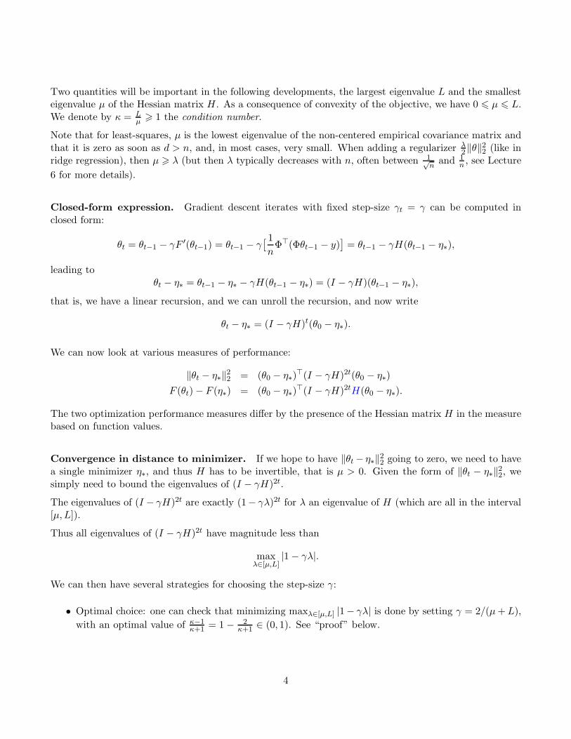
We can then have several strategies for choosing the step-size γ:

• Optimal choice: one can check that minimizing maxλ∈[µ,L] |1− γλ| is done by setting γ = 2/(µ+L),

with an optimal value of κ−1κ+1 = 1− 2

κ+1 ∈ (0, 1). See “proof” below.

4

γ1/L 1/µ

max|1− γL|, |1− γµ|

|1− γµ|

|1− γL|

2/(L+ µ)

• Choice independent of µ: with the simpler (slightly smaller) choice γ = 1/L, we get maxλ∈[µ,L] |1 −γλ| = (1− µ

L) = (1− 1

κ), which is only sligthly larger than the value for the optimal choice.

With the weaker choice γ = 1/L, we get:

‖θt − η∗‖22 6(

1− 1

κ

)2t‖θ0 − η∗‖22,

which is often referred to as exponential, geometric, or also linear convergence.

! The denomination “linear” is sometimes confusing and corresponds to a number of significant digitsthat grows linearly with the number of iterations.

We can further bound(

1− 1κ

)2t6 exp(−1/κ)2t = exp(−2t/κ), and thus the characteristic time of conver-

gence is of order κ. We will often make the calculation ε = exp(−2t/κ) ⇔ t = κ2 log

1ε. Thus, for a relative

reduction of squared distance to optimum of ε, we need at most t = κ2 log

1εiterations.

For κ = +∞, then the result remains true, but simply say that for all minimizers ‖θt − η∗‖22 6 ‖θ0 − η∗‖22,which is a good sign (the algorithm does not move away from minimizers) but not indicative of any formof convergence. We will need to use a different criterion.

Convergence in function values. Using the same step-size as above, and using the upper-bound oneigenvalues of (I − γH)2t, we get

F (θt)− F (η∗) 6(

1− 1

κ

)2t[F (θ0)− F (η∗)].

When κ < ∞ (that is, µ > 0), then we also obtain linear convergence for this criterion, but when κ = ∞,this is non-informative.

In order to obtain a convergence rate, we will need to bound the eigenvalues of (I − γH)2tH instead of(I − γH)2t. The key difference is that for eigenvalues λ of H which are close to zero (1 − γλ)2t does nothave a strong contracting effect, but they count less as they are multiplied by λ in the bound.

We can now make this trade-off precise, for γ 6 1/L, as∣∣λ(1− γλ)2t

∣∣ 6 λ exp(−γλ)2t = λ exp(−2tγλ)

=1

2tγ2tγλ exp(−2tγλ) 6

1

2tγsupα>0

α exp(−α) =1

2etγ6

1

4tγ,

5

where we used that αe−α is maximized over R+ at α = 1 (as the derivative e−α(1− α)).

This leads to

F (θt)− F (η∗) 61

4tγ‖θ0 − η∗‖22.

We can make the following observations:

• ! The convergence results in exp(−t/κ) for invertible Hessians or 1/t in general are only upper-bounds! It is good to understand the gap between the bounds and the actual performance, as this ispossible for quadratic objective functions.

For the exponentially convergent case, the lowest eigenvalue µ dictates the rate for all eigenvalues.So if the eigenvalues are well-spread (or if only one eigenvalue is very small), there can be quite astrong discrepancy between the bound and the actual behavior.

For the rate in 1/t, the bound in eigenvalues is tight when tγλ is of order 1, namely when λ is of order1/(tγ). Thus, in order to see an O(1/t) convergence rate in practice, we need to have sufficientlymany small eigenvalues, and as t grows, we often go to a local linear convergence phase where thesmallest non zero eigenvalue of H kicks in. See simulations and exercice below.

– Exercice: Let µ+ be the smallest non-zero eigenvalue of H. Show that gradient descent islinearly convergence with the contracting rate (1− µ+/L).

• Can an algorithm having the same access to oracles of F do better?

If we have access to matrix-vector products with the matrix Φ, then conjugate gradient can be usedwith convergence rates in exp(−t/

√κ) and 1/t2 (see [3]). With only access to gradients of F (which

is a bit weaker) Nesterov acceleration (see below) will also lead to the same convergence rates, whichare then optimal (for a sense to be defined later).

• Can we extend beyond least-squares? The convergence results above will generalize to convex func-tions (see Section 2.2), but with less direct proofs. Non-convex objectives are discussed in Section 2.6

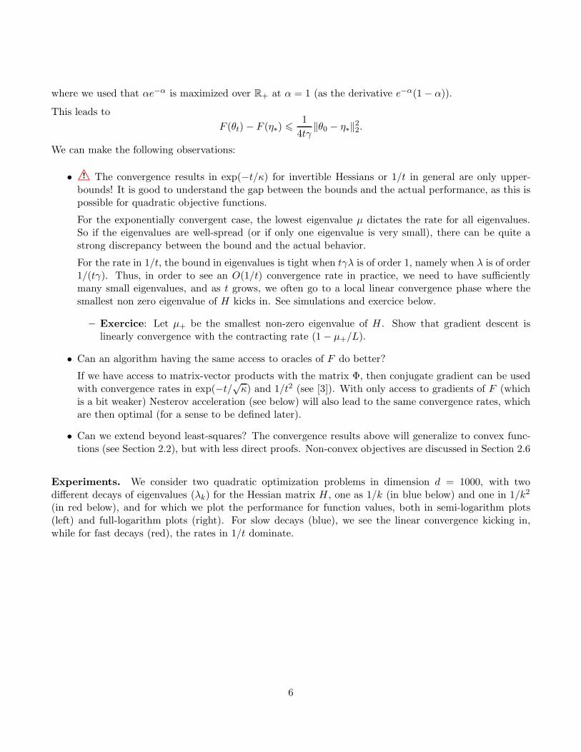
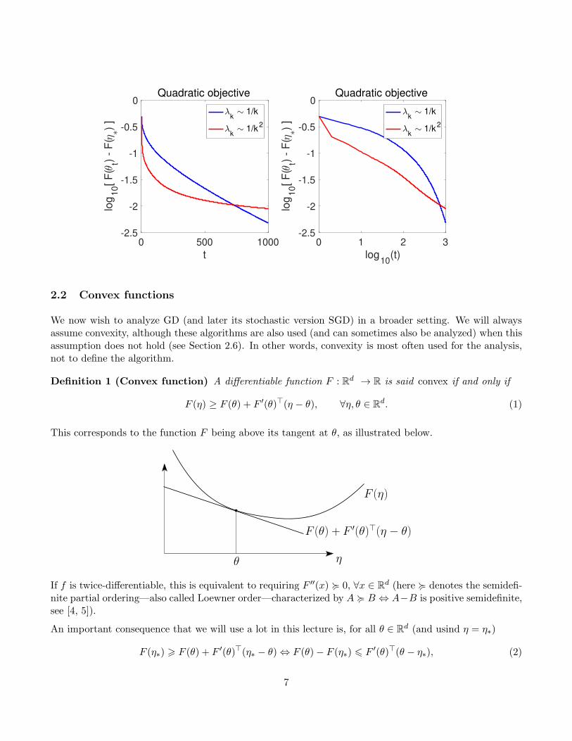
Experiments. We consider two quadratic optimization problems in dimension d = 1000, with twodifferent decays of eigenvalues (λk) for the Hessian matrix H, one as 1/k (in blue below) and one in 1/k2

(in red below), and for which we plot the performance for function values, both in semi-logarithm plots(left) and full-logarithm plots (right). For slow decays (blue), we see the linear convergence kicking in,while for fast decays (red), the rates in 1/t dominate.

6

0 500 1000

t

-2.5

-2

-1.5

-1

-0.5

0lo

g1

0[

F(

t) -

F(

) ]

Quadratic objective

k 1/k

k 1/k

2

0 1 2 3

log10

(t)

-2.5

-2

-1.5

-1

-0.5

0

log

10[

F(

t) -

F(

) ]

Quadratic objective

k 1/k

k 1/k

2

2.2 Convex functions

We now wish to analyze GD (and later its stochastic version SGD) in a broader setting. We will alwaysassume convexity, although these algorithms are also used (and can sometimes also be analyzed) when thisassumption does not hold (see Section 2.6). In other words, convexity is most often used for the analysis,not to define the algorithm.

Definition 1 (Convex function) A differentiable function F : Rd → R is said convex if and only if

F (η) ≥ F (θ) + F ′(θ)⊤(η − θ), ∀η, θ ∈ Rd. (1)

This corresponds to the function F being above its tangent at θ, as illustrated below.

η

F (η)

θ

F (θ) + F′(θ)⊤(η − θ)

If f is twice-differentiable, this is equivalent to requiring F ′′(x) < 0, ∀x ∈ Rd (here < denotes the semidefi-

nite partial ordering—also called Loewner order—characterized by A < B ⇔ A−B is positive semidefinite,see [4, 5]).

An important consequence that we will use a lot in this lecture is, for all θ ∈ Rd (and usind η = η∗)

F (η∗) > F (θ) + F ′(θ)⊤(η∗ − θ) ⇔ F (θ)− F (η∗) 6 F ′(θ)⊤(θ − η∗), (2)

7

that is the distance to optimum in function values is upperbounded by a function of the gradient.

A more general definition of convexity is that ∀x, y ∈ Rd and α ∈ [0, 1],

F (αη + (1− α)θ) 6 αF (η) + (1− α)F (θ).

• Exercise: show that if F is differentiable, this is equivalent to our definition. The following inequalityappears frequently in the proofs involving convexity.

Proposition 1 (Jensen’s inequality) If F : Rd → R is convex and µ is a probability measure on Rd,

then

F( ∫

θdµ(θ))

6

∫

F (θ)dµ(θ).

In words: “the image of the average is smaller than the average of the images”.

The class of convex functions satisfies the following stability properties (proofs left as an exercise):

• If (Fj)j∈[m] are convex and (αj)j∈[m] are nonnegative, then∑m

j=1 αjFj is convex.

• If F : Rd → R is convex and A : Rd′ → Rd is linear then F A : Rd′ → R is convex.

Example. Problems of the form in Eq. (1) are convex if the loss ℓ is convex in the second variable, fθ(x)is linear in θ, and Ω is convex.

It is also worth emphasizing on the following property (immediate from the definition).

Proposition 2 Assume that F : Rd → R is convex and differentiable. Then η∗ ∈ Rd is a global minimizer

of F if and only ifF ′(η∗) = 0.

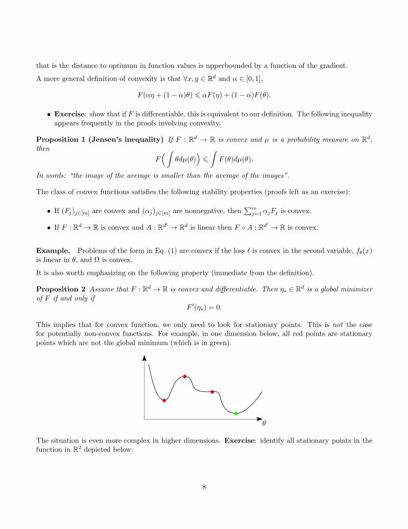
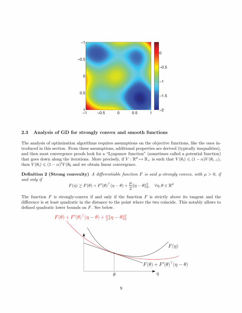
This implies that for convex function, we only need to look for stationary points. This is not the casefor potentially non-convex functions. For example, in one dimension below, all red points are stationarypoints which are not the global minimum (which is in green).

θ

The situation is even more complex in higher dimensions. Exercise: identify all stationary points in thefunction in R

2 depicted below.

8

1 0.5 0 0.5 1

1

0.5

0

0.5

1 2

1.5

1

0.5

0

2.3 Analysis of GD for strongly convex and smooth functions

The analysis of optimization algorithms requires assumptions on the objective functions, like the ones in-troduced in this section. From these assumptions, additional properties are derived (typically inequalities),and then most convergence proofs look for a “Lyapunov function” (sometimes called a potential function)that goes down along the iterations. More precisely, if V : Rd 7→ R+ is such that V (θt) 6 (1− α)V (θt−1),then V (θt) 6 (1− α)tV (θ0 and we obtain linear convergence.

Definition 2 (Strong convexity) A differentiable function F is said µ-strongly convex, with µ > 0, ifand only if

F (η) ≥ F (θ) + F ′(θ)⊤(η − θ) +µ

2‖η − θ‖22, ∀η, θ ∈ R

d

The function F is strongly-convex if and only if the function F is strictly above its tangent and thedifference is at least quadratic in the distance to the point where the two coincide. This notably allows todefined quadratic lower bounds on F . See below.

η

F (η)

θ

F (θ) + F ′(θ)⊤(η − θ)

F (θ) + F ′(θ)⊤(η − θ) + µ2‖η − θ‖2

2

9

For twice differentiable functions, this is equivalent to F ′′ < µI (see [1]).

• Exercise: show that if F is convex, then F + µ2 ‖ · ‖22 is µ-strongly convex.

• In machine learning problems, with linear models, so that the empirical risk is convex, strong convex-ity most often comes from the regularizer (and thus µ decays with n), leading to condition numbersthat grow with n.

This property implies that F admits a unique minimizer η∗, which is characterized by F ′(η∗) = 0. Moreover,this guarantees that the gradient is large when a point is far from optimality:

Lemma 1 (Lojasiewicz inequality) If F is differentiable and µ-strongly convex with minimizer η∗, thenit holds

‖F ′(θ)‖22 ≥ 2µ(F (θ)− F (η∗)), ∀θ ∈ Rd.

Proof The right-hand side in Definition 2 is strongly convex in η and minimized with η = θ − 1µF ′(θ).

Plugging this value into the bound and taking η = η∗ in the left-hand side we get

F (η∗) ≥ F (θ)− 1

µ‖F ′(θ)‖22 +

1

2µ‖F ′(θ)‖22 = F (θ)− 1

2µ‖F ′(θ)‖22.

The conclusion follows by rearranging.

Definition 3 (Smoothness) A differentiable function F is said L-smooth if and only if

|F (η) − F (θ)− F ′(θ)⊤(η − θ)| 6 L

2‖θ − η‖2, ∀θ, η ∈ R

d

This is equivalent to F having a L-Lipschitz gradient, i.e., ‖F ′(θ) − F ′(η)‖22 6 ‖θ − η‖22, ∀θ, η ∈ Rd. For

twice differentiable functions, this is equivalent to −LI 4 F ′′(θ) 4 LI (see [1]).

Note that when F is convex and L-smooth, we have a quadratic upper-bound which is tight at any givenpoint (strong convexity implies the corresponding lower bound). See below.

η

F (η)

θ

F (θ) + F′(θ)⊤(η − θ)

F (θ) + F′(θ)⊤(η − θ) + L

2‖η − θ‖2

2

10

When a function is both smooth and strongly convex, we denote by κ = L/µ > 1 its condition number.See examples below: the condition number impacts the shapes of the level sets).

(small κ = L/µ) (large κ = L/µ)

The performance of gradient descent will depend on this condition number (see steepest descent below, thatis, gradient descent with exact line search): with small condition number (left), we get fast convergence,while for a large condition number (right), we get oscillations.

(small κ = L/µ) (large κ = L/µ)

• For machine learning problems, for linear predictions and smooth losses (square or logistic), then wehave smooth problems. If we use a squared ℓ2-regularizer

µ2 regularizer, we get at µ-strongly convex

problem. Note that when using regularization, as explained in Lectures 2 and 3, the value of µ decayswith n, typically between 1/n and 1/

√n, leading to condition numbers between

√n and n.

In this context, gradient descent on the empirical risk, is often called a “batch” technique.

In the next theorem, we show that gradient descent converges exponentially for such problems.

Theorem 1 (Convergence of GD for strongly convex functions) Assume that F is L-smooth andµ-strongly convex. Choosing γt = 1/L, the iterates (θt)t≥0 of GD on F satisfy

F (θt)− F (η∗) ≤ exp(−tµ/L)(F (θ0)− F (η∗)).

11

Proof By smoothness, we have the following descent property, with γt = 1/L,

F (θt) = F (θt−1−F ′(θt−1/L) 6 F (θt−1) + F ′(θt−1)⊤(−F ′(θt−1)/L) +

L

2‖−F ′(θt−1)/L‖22

= F (θt−1)− ‖F ′(θt−1)‖22/L+1

2L‖F ′(θt−1)‖22.

Rearranging, we get

F (θt)− F (η∗) 6 (F (θt−1)− F (η∗))−1

2L‖F ′(θt−1)‖22.

Using Lemma 1, it follows

F (θt)− F (η∗) 6 (1− µ/L)(F (θt−1)− F (η∗)) 6 exp(−µ/L)(F (θt−1)− F (η∗)).

We conclude by a recursion.

• We necessarily have µ 6 L. The ratio κ := L/µ is called the condition number.

• If we only assume that the function is smooth and convex (not strongly convex), then GD withconstant step-size γ = 1/L also converges when a minimizer exists, but at a slower rate in O(1/t).See proof below.

• Choosing the step-size only requires an upper bound L on the smoothness constant (in case it isover-estimated, the convergence rate only degrades slightly).

• Note that gradient descent is adaptive to strong convexity: the exact same algorithm applies toboth strongly convex and convex cases, and the two bounds apply. This adaptivity is important inpractice, as often, locally around the global optimum, the strong convexity constant converges tothe minimal eigenvalue of the Hessian at η∗, which can very significantly larger than µ (the globalconstant).

• Exercise: compute all constants for ℓ2-regularized logistic regression.

• Fenchel conjugate: given some convex function F : Rd → R, an important tool is the Fenchelconjugate F ∗ defined as F ∗(α) = supθ∈Rd α⊤θ − F (θ). This is crucial when dealing with convexduality (which we will not cover in this lecture); see [4] for details.

2.4 Analysis of GD for convex and smooth functions ()

In order to obtain the 1/t convergence rate without strong-convexity, we will need an extra property ofconvex smooth functions, sometimes called “co-coercivity”. This is an instance of inequalities that we needto use to circumvent the lack of closed form for iterations.

Proposition 3 If F is a convex L-smooth function on Rd, then for all θ, η ∈ R

d, we have:

1

L‖F ′(θ)− F ′(η)‖22 6

[F ′(θ)− F ′(η)

]⊤(θ − η).

Moreover, we have: F (θ) > F (η) + F ′(η)⊤(θ − η) + 12L‖F ′(θ)− F ′(η)‖2.

12

Proof We wil show the second inequality, which implies the first one by applying it twice with η and θswapped, and summing them.

• Define H(θ) = F (θ)− θ⊤F ′(η). The function H : Rd → R is convex with global minimum at η, sinceH ′(θ) = F ′(θ)− F ′(η), which is equal to zero for θ = η. The function H is also L-smooth.

• We can apply the definition of smoothness: H(η) 6 H(θ− 1LH ′(θ)) 6 H(θ) + H ′(θ)⊤(− 1

LH ′(θ)) +

L2 ‖− 1

LH ′(θ)‖22, which is thus less than H(θ)− 1

2L‖H ′(θ)‖22• This leads to F (η) − η⊤F ′(η) 6 F (θ) − θ⊤F ′(η) − 1

2L‖F ′(θ) − F ′(η)‖22, which leads to the desiredinequality by shuffling terms.

Following [6], the Lyapunov function that we will choose is

Vt(θt) = t[F (θt)− F (η∗)] +L

2‖θt − η∗‖22,

and our goal is to show that it decays along iterations. We get:

Vt(θt)− Vt−1(θt−1) = t[F (θt)− F (θt−1)] + F (θt)− F (η∗) +L

2‖θt − η∗‖22 −

L

2‖θt−1 − η∗‖22

In order to bound it, we use:

• We use F (θt)− F (θt−1) 6 − 12L‖F ′(θt−1‖22 like in the proof of Theorem 1

• We use F (θt)− F (η∗) 6 F ′(θt−1)⊤(θt−1 − η∗), as a consequence of convexity (function above the

tangent at θt−1), as in Eq. (2).

• We get L2 ‖θt − η∗‖22 − L

2 ‖θt−1 − η∗‖22 = −Lγ(θt−1 − η∗)⊤F ′(θt−1) +Lγ2

2 ‖F ′(θt−1)‖22 by expanding thesquare.

This leads to, with γ = 1/L:

Vt(θt)− Vt−1(θt−1) 6 t[− 1

2L‖F ′(θt−1‖22

]+ F ′(θt−1)

⊤(θt−1 − η∗)−Lγ(θt−1 − η∗)⊤F ′(θt−1) +

Lγ2

2‖F ′(θt−1)‖22

= − t− 1

2L‖F ′(θt−1‖22 6 0,

which leads to

t[F (θt)− F (η∗)] 6 Vt(θt) 6 V0(θ0) =L

2‖θ0 − η∗‖22,

and thus F (θt)− F (η∗) 6L2t‖θ0 − η∗‖22.

The proof above is on purpose mysterious: the choice of Lyapunov function seems arbitrary at first, but allinequalities lead to nice cancellations. These proofs are sometimes hard to design. For a very interesting lineof work trying to automate these proofs, see https://francisbach.com/computer-aided-analyses/.

13

2.5 Beyond gradient descent ()

While gradient descent is the simplest algorithm with a simple analysis, there are multiple extensions thatwe will only briefly mention (see more details in [7, 8]):

• Nesterov acceleration: For convex functions, a simple modification of gradient descent allows toobtain better convergence rates. The algorithm is as follows, and is based on updating iterates:

θt = ηt−1 −1

LF ′(ηt−1)

ηt = θt +t− 1

t+ 2(θt − θt−1).

This simple modification dates back to Nesterov in 1983, and leads to the following convergence rate

F (θt)− F (η∗) 62L‖θ0−η∗‖2

(t+1)2.

For strongly convex functions, the algorithm has a similar form as for convex functions, but with allcoefficients which are independent from t:

θt = ηt−1 −1

Lg′(ηt−1)

ηt = θt +1−

√

µ/L

1 +√

µ/L(θt − θt−1),

and the convergence rate is F (θt)−F (η∗) 6 L‖θ0 − η∗‖2(1−√

µ/L)t, that is the characteristic timeto convergence goes from κ to κ. If κ is large (typically of order

√n or n for machine learning), the

gains are substantial. In practice, this leads to significant improvements.

Moreover, the last two rates are known to be optimal for the considered problems: for algorithmsthat access gradient and combine them linearly to select a new query point, it is not possible to havebetter dimension-independent rates. See [8] for more details.

• Newton methods: Given θt−1, the Newton method minimizes the second-order Taylor expansionaround θt−1

F (θt−1) + F ′(θt−1)⊤(θ − θt−1) +

1

2(θ − θt−1)

⊤F ′′(θt−1)⊤(θ − θt−1),

which leads to θt = θt−1 − F ′′(θt−1)−1F ′(θt−1), which is an expansive iteration, as the running-time

complexity is O(d3) in general to solve the linear system. It leads to local quadratic convergence: If‖θt−1 − θ∗‖ small enough, for some constant C, we have (C‖θt − θ∗‖) = (C‖θt−1 − θ∗‖)2. See [4] formore details, and for conditions for global convergence.

Note that for machine learning problems, quadratic convergence may be an overkill compared to thecomputational complexity of each iteration, since cost functions are averages of n terms and naturallyhave some uncertainty of order O(1/

√n).

• Proximal gradient descent (): Many optimization problems are said “composite”, that is, theobjective function F is the sum of a smooth function G and a non-smooth function H (such as anorm). It turns out that a simple modification of gradient descent allows to benefit from the fastconvergence rates of smooth optimization.

14

For this, we need to first see gradient descent as a proximal method. Indeed, one may see the iterationθt = θt−1 − 1

LG′(θt−1), as

θt = arg minθ∈Rd

G(θt−1) + (θ − θt−1)⊤G′(θt−1) +

L

2‖θ − θt−1‖22,

where, for a L-smooth function G, the objective function above is an upper-bound of G(θ) which istight at θt−1.

While this reformulation does not bring much for gradient descent, we can extend this to the com-posite problem, and consider the iteration

θt = arg minθ∈Rd

G(θt−1) + (θ − θt−1)⊤G′(θt−1) +

L

2‖θ − θt−1‖22 +H(θ),

where H is left as is. It turns out that the convergence rates for G + H are the same as smoothoptimization, with potential acceleration [8, 9].

The crux is to be able to compute the step above, that is minimize with respect to θ functions ofthe form L

2 ‖θ − η‖22 +H(θ). When H is the indicator function of a convex set (which is equal to 0inside the set, and +∞ otherwise), we get projected gradient descent. When H is the ℓ1-norm, that isH = λ‖·‖2, this can be shown to be soft-thresholding step, as for each coordinate θi = (|ηi|−λ/L)+

ηi|ηi|

(proof left as an exercise).

2.6 Non-convex objective functions ()

For smooth potentially non convex objective functions, the best one can hope for is to converge to astationary point θ such that F ′(θ) = 0. The proof below provides the weaker result that at least oneiterate has a small gradient. Indeed, using the same Taylor expansion as the convex case (which is stillvalid), we get

F (θt) 6 F (θt−1)−1

2L‖F ′(θt−1)‖22,

leading to, summing the inequalities above for all iterations between 1 and t, we get:

1

t

t∑

s=1

‖F ′(θs−1)‖22 6F (θ0)− F (η∗)

t.

Thus there has to be one s in 0, . . . , t− 1 for which ‖F ′(θs)‖22 6 O(1/t).

3 Gradient methods on non-smooth problems

We now relax our assumptions and only require Lipschitz continuity, in addition to convexity. The rateswill be slower, but the extension to stochastic gradients easier.

Definition 4 (Lipschitz function) A function F : Rd → R is said B-Lipschitz-continuous if and onlyif

|F (η) − F (θ)| 6 B‖η − θ‖2, ∀θ, η ∈ Rd.

15

• Exercise: show that if F is differentiable, this is equivalent to the assumption ‖F ′(θ)‖2 6 B, ∀θ ∈ Rd.

Without additional assumptions, this setting is usually referred to as non-smooth optimization.

• We can apply non-smooth optimization to objective functions which are not differentiable. For convexLipschitz-continuous objectives, the function is almost everywhere differentiable. In points where itis not, then one can define the set of slopes of lower-bounding tangents as the subdifferential, and anyelement of it as a subgradient. The gradient descent iteration is then meant as using any subgradientinstead of F ′(θt−1). The method is then referred to as the subgradient method (it is not a descentmethod anymore, that is, the function values may go up once in a while).

The method can be in particular applied to the hinge loss.

3.1 Convergence rate of the subgradient method

Theorem 2 (Convergence of the subgradient method) Assume that F is convex, B-Lipschitz andadmits a minimizer η∗ that satisfies ‖η∗ − θ0‖2 6 D. By chosing γt =

D

B√tthen the iterates (θt)t≥0 of GD

on G satisfy

min06s6t−1

F (θs)− F (η∗) 6 DB2 + log(t)√

t.

Proof We look at how θt approaches η∗, that is, we try to use ‖θt − η∗‖22 as a Lyapunov function. Wehave:

‖θt − η∗‖22 = ‖θt−1 − γtF′(θt−1)− η∗‖22 = ‖θt−1 − η∗‖22 − 2γtF

′(θt−1)⊤(θt−1 − η∗) + γ2t ‖F ′(θt−1)‖22.

Combining this with the convexity inequality F (θt−1) − F (η∗) 6 F ′(θt−1)⊤(θt−1 − η∗) from Eq. (2), it

follows (also using the boundedness of gradients):

‖θt − η∗‖22 6 ‖θt−1 − η∗‖22 − 2γt[F (θt−1)− F (η∗)] + γ2tB2.

and thus, by isolating the distance to optimum in function values:

γt(F (θt−1)− F (η∗)) 61

2

(

‖θt−1 − η∗‖22 − ‖θt − η∗‖22)

+1

2γ2tB

2. (3)

It is sufficient to sum these inequalities to get, for any η∗ ∈ Rd,

1∑t

s=1 γs

t∑

s=1

γs (F (θs−1)− F (η∗)) 6‖θ0 − η∗‖222∑t

s=1 γs+B2

∑ts=1 γ

2s

2∑t

s=1 γs.

The left-hand side is larger than min06s6t−1(F (θs) − F (η∗)) (trivially) and than F (θt) − F (η∗) whereθt = (

∑ts=1 γsθs−1)/(

∑ts=1 γs) by Jensen’s inequality.

The upper bound goes to 0 if∑t

s=1 γs goes to ∞ (to forget the initial condition, sometimes called the“bias”) and γt → 0 (to decrease the “variance” term). Let us choose γs = τ/

√s for some τ > 0. By using

the series-integral comparisons below, we get the bound

min06s6t−1

(F (θs)− F (η∗)) 61√t

(

D2/τ + τB2(1 + log(t)))

.

16

We choose τ = D/B (which is suggested by optimizing the previous bound when log(t) = 0) which leadsto the result.

In the proof, we used the following series-integral comparisons for decreasing functions:

t∑

s=1

1√s≥

∫ t

0

ds√s+ 1

=[

2√s+ 1

]t

0= 2

√t+ 1− 2 >

1

2

√t

andt∑

s=1

1

s6 1 +

t∑

s=2

1

s6 1 +

∫ t

0

ds

s= 1 + log(t).

• The previous proof scheme is very flexible. It can be extended in the following directions

– No need to know in advance an upper-bound D on the distance to optimum, we then get with

the same step-size γt =D

B√ta rate of the form BD√

t

(‖θ0−η∗‖22

D2 + (1 + log(t)))

.

– Constrained minimization over a convex set (we then insert a projection step at each iteration);

– Non-differentiable convex and Lipschitz objective functions (using sub-gradients, i.e. any vectorsatisfying Eq. (1) in place of F ′(θt));

– Non-Euclidean geometry (for instance multiplicative instead of additive updates), using “mirrordescent”.

– Often the uniformly averaged iterate is used, as 1t

∑t−1s=0 θs. Convergence rates (without the

log t factor) can be obtained using Abel summation formula (see https://francisbach.com/

integration-by-parts-abel-transformation/).

– Stochastic gradients, as seen below.

• Exercise: compute all constants for ℓ2-regularized logistic regression.

4 Convergence rate of SGD

For machine learning problems, at each iteration, the gradient descent algorithm requires to compute a“full” gradient F ′(θt−1) which could be costly. An alternative is to instead only compute unbiased stochasticestimations of the gradient gt(θt−1), i.e., such that E[gt(θt−1)|θt−1] = F ′(θt−1), which could be much fasterto compute.

Note that we need to condition over θt−1 because θt−1 encapsulates all the randomness due to past itera-tions, and we only require “fresh” randomness at time t.

Somewhat surprisingly, this unbiasedness does not need to be coupled with a vanishing variance: whilethere are always errors in the gradient, the use of a decreasing step-size will ensure convergence.

This leads to the following algorithm.

Algorithm 2 (Stochastic gradient descent (SDG)) Choose step-size sequence (γt)t≥0, pick θ0 ∈ Rd

and for t ≥ 0, letθt+1 = θt − γtgt(θt).

17

SGD in machine learning. There are two ways to use SGD for supervised machine learning:

• Empirical risk minimization: If F (θ) = 1n

∑ni=1 ℓ(yi, fθ(xi)) then at iteration t we can choose uni-

formly at random i(t) ∈ 1, . . . , n and define gt as the gradient of θ 7→ ℓ(yi(t), fθ(xi(t))). There exists“mini-batch” variants where at each iteration, the gradient is averaged over a random subset of theindices. We then converge to a minimizer η∗ of the empirical risk.

Note here that since we sample with replacement, a given function will be selected several times.

• Population risk minimization: If F (θ) = E[ℓ(y, fθ(x))] then at iteration t we can take a fresh sample(xt, yt) and define gt as the gradient of θ 7→ ℓ(yt, fθ(xt)), for which, if we swap the orders of expectationand differentiation, we get the unbiasedness. Note here that to preserve the unbiasedness, only asingle pass is allowed (otherwise, this would create dependencies that would break it).

Here, we directly minimize the (generalization) risk. The counterpart is that if we only have nsamples, then we can only run n SGD iterations, and when n grows, the iterates will converge to aminimizer θ∗ of the expected risk.

We can study the two situations above using the latter one, by considering the empirical risk as theexpectation with respect to the empirical distribution of the data.

! SGD is not a descent method

Under the same assumptions on the objective, we now study SGD . We assume the following:

• (H1) unbiased gradient: E[gt(θt−1)|θt−1] = F ′(θt−1), ∀t,

• (H2) bounded gradient: ‖gt(θt−1)‖22 6 B2, ∀t almost surely

Theorem 3 (Convergence of SGD) Assume that F is convex, B-Lipschitz and admits a minimizerθ∗ that satisfies ‖θ∗ − θ0‖2 6 D. Assume that the stochastic gradients satisfy (H1-2). Then, choosingγt = (D/B)/

√t, the iterates (θt)t≥0 of SGD on F satisfy

E

[

F (θt)− F (θ∗)]

6 DB2 + log(t)√

t.

where θt = (∑t

s=1 γsθs−1)/(∑t

s=1 γs).

Proof We follow essentially the same proof as in the deterministic case, adding some expectations at wellchosen places.

E

[

‖θt − θ∗‖22]

= E

[

‖θt−1 − γtgt(θt−1)− θ∗‖22]

= E

[

‖θt−1 − θ∗‖22]

− 2γtE[

gt(θt−1)⊤(θt−1 − θ∗)

]

+ γ2t E[

‖gt(θt−1)‖22]

6 E

[

‖θt−1 − θ∗‖22]

− 2γtE[

F ′(θt−1)⊤(θt−1 − θ∗)

]

+ γ2tB2.

18

Above, the subtle part is the expectation

E

[

gt(θt−1)⊤(θt−1 − θ∗)

]

= E

[

E

[

gt(θt−1)⊤(θt−1 − θ∗)

∣∣∣θt−1

]]

= E

[

E

[

gt(θt−1)∣∣∣θt−1

]⊤(θt−1 − θ∗)

]

= E

[

F ′(θt−1)⊤(θt−1 − θ∗)

]

.

Thus, combining with the convexity inequality F (θt−1) − F (θ∗) 6 F ′(θt−1)⊤(θt−1 − θ∗) from Eq. (2), it

follows

γtE[F (θt−1)− F (θ∗)] 61

2

(

E[‖θt−1 − θ∗‖22

]− E

[‖θt − θ∗‖22

])

+1

2γ2tB

2. (4)

Except for the expectations, this is the same bound that Eq. (3) so we can conclude as in the proof ofTheorem 2, mutatis mutandis. We state our bound in terms of the average iterates because the cost offinding the best iterate could be high in comparison to that of evaluating a stochastic gradient.

• Many authors consider the projected version of the algorithm where after the gradient step, weorthogonally project onto the ball of radius D and center θ0. The bound is then exactly the same.

• The result that we obtain, when applied to single pass SGD, is a generalization bound that is, after then iterations, we have an excess risk proportion to 1/

√n, corresponding to the excess risk compared

to the best predictor fθ.

This is to be compared to using results from Lecture 3 (uniform deviation bounds) and non-stochasticgradient descent. It turns out that the estimation error due to having n observation is exactly thesame as the generalization bound obtained by SGD, but we need to add on top the optimizationerror proportional to 1/

√t (with the same constants). The bounds match if t = n, that is, we run

n iterations of gradient descent on the empirical risk. This leads to a running time complexity ofO(tnd) = O(n2d) instead of O(nd) using SGD, hence the strong gains in using SGD.

• The bound in O(BD/√t) is optimal for this class of problem. That is, as shown for example in [10],

among all algorithms that can query stochastic gradients, having a better convergence rate (up tosome constants) is impossible.

• As opposed to the deterministic case, the use of smoothness does not lead to significantly betterresults.

4.1 Strongly convex problems ()

We consider the regularized problem G(θ) = F (θ)+ µ2 ‖θ‖22, with the same assumption as above, and started

at θ0 = 0. The SGD iteration is then:

θt = θt−1 − γt[gt(θt−1) + µθt−1

]. (5)

We then have

19

Theorem 4 (Convergence of SGD for strongly-convex problems) Assume that F is convex, B-Lipschitz and that G + µ

2‖ · ‖22 admits a (necesary unique) minimizer θ∗. Assume that the stochasticgradient g satisfies (H1-2). Then, choosing γt = 1/(µt), the iterates (θt)t≥0 of SGD from Eq. (5) satisfy

E

[

F (θt)− F (θ∗)]

62B2(1 + log t)

µt

where θt = (∑t

s=1 γsθs−1)/(∑t

s=1 γs).

Proof The beginning of the proof is essentially the same as for convex problems, leading to (with the newterms in blue):

E

[

‖θt − θ∗‖22]

= E

[

‖θt−1 − γt(gt(θt−1)+µθt−1)− θ∗‖22]

= E

[

‖θt−1 − θ∗‖22]

− 2γtE[

(gt(θt−1)+µθt−1)⊤(θt−1 − θ∗)

]

+ γ2t E[

‖gt(θt−1)+µθt−1‖22]

.

From the iterations, we see that θt = (1−γtµ)θt−1+γtµ[− 1

µgt(θt−1)

]is a convex combination of gradients

divided by −µ, and thus ‖gt(θt−1) + µθt−1‖22 is always less than 4B2. Thus

E

[

‖θt − θ∗‖22]

6 E

[

‖θt−1 − θ∗‖22]

− 2γtE[

G′(θt−1)⊤(θt−1 − θ∗)

]

+ 4γ2tB2.

Therefore, combining with the strong convexity inequalityG(θt−1)−G(η∗)+µ2 ‖θt−1 − θ∗‖22 6 G′(θt−1)

⊤(θt−1−θ∗) it follows

γtE[F (θt−1)− F (θ∗)] 61

2

(

(1−γtµ)E‖θt−1 − θ∗‖2 − E‖θt − θ∗‖2)

+ 2γ2tB2,

and thus, now using the specific step-size choice:

E[F (θt−1)− F (θ∗)] 61

2

(

(γ−1t − µ)E‖θt−1 − θ∗‖2 − γ−1

t E‖θt − θ∗‖2)

+ 2γtB2,

=1

2

(

µ(t− 1)E‖θt−1 − θ∗‖2 − µtE‖θt − θ∗‖2)

+2B2

µt.

Thus, summing between all indices between 1 and t, and using the bound∑t

s=11s6 1 + log t.

• For smooth problems, we can show a similar bound of the form O(κ/t). For quadratic problems,constant step-sizes can be used with averaging, leading to improved convergence rates [11].

• The bound in O(B2/µt) is optimal for this class of problem. That is, as shown for example in [10],among all algorithms that can query stochastic gradients, having a better convergence rate (up tosome constants) is impossible.

• We note that for the same regularized problem, we could use a step size proportion to DB/√t and

obtain a bound proportional to DB/√t, which looks worse thatn B2/(µt), but can in fact be better.

Note also the loss of adaptivity: the step-size now depends on the difficulty of the problem (this wasnot the case for deterministic gradient descent).

See experiments below for illustrations.

20

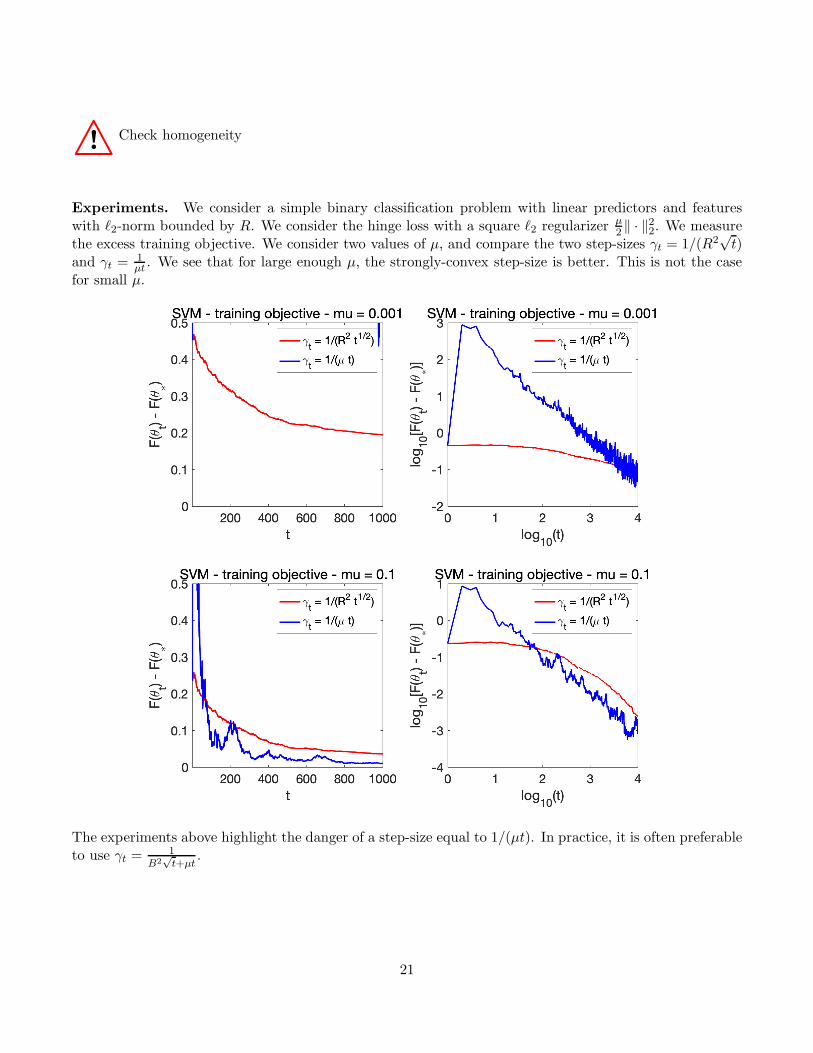
! Check homogeneity

Experiments. We consider a simple binary classification problem with linear predictors and featureswith ℓ2-norm bounded by R. We consider the hinge loss with a square ℓ2 regularizer µ

2 ‖ · ‖22. We measurethe excess training objective. We consider two values of µ, and compare the two step-sizes γt = 1/(R2

√t)

and γt =1µt. We see that for large enough µ, the strongly-convex step-size is better. This is not the case

for small µ.

The experiments above highlight the danger of a step-size equal to 1/(µt). In practice, it is often preferableto use γt =

1B2

√t+µt

.

21

4.2 Variance reduction ()

We consider a finite sum F (θ) = 1n

∑ni=1 fi(θ), where each fi is R

2-smooth (for example logistic regressionwith features bounded by R in ℓ2-norm), and which is such that F is µ-strongly convex.

Using SGD, the convergence rate can be shown to to O(κ/t), with iterations of complexity O(d), while forGD, the convergence rates is O(exp(−t/κ)), but each iteration has complexity O(nd). We now present aresult allowing to get exponential convergence with an iteration cost which is O(d).

The idea is to use a form of variance reduction, which is made possible by keeping in memory past gradients.

We denote by z(t)i ∈ R

d the version of gradient i stored at time t.

The SAGA algorithm [12] is as follows.

• At every iteration, an index i(t) is selected uniformly at random in 1, . . . , n, and we perform the

iteration θt = θt−1 − γ[

f ′i(t)(θt−1) +

1

n

n∑

i=1

z(t−1)i − z

(t−1)i(t)

]with z

(t)i(t) = f ′

i(t)(θt−1) and all others zti left

unchanged (i.e., the same as z(t−1)i ).

The idea behind variance reduction is that if the random variable z(t−1)i(t) (only considering the source

of randomness coming from i(t) is positively correlated with f ′i(t)(θt−1), then the variance is reduced,

and larger step-sizes can be used.

As the algorithm converges, then z(t)i converges to f ′

i(η∗), and then the update tends to have zerovariance, and thus a constant step-size allows to obtain convergence. The key is then to show

simultaneously that θt converges to η∗ and that all z(t)i converge to f ′

i(η∗), all at the same speed.

Theorem 5 (Convergence of SAGA) If initializing with z(0)i = f ′

i(θ0), we have

E[‖θt − η∗‖22

]6

(

1−min 1

3n,3µ

4R2)t(

1 +n

4

)‖θ0 − η∗‖22.

Proof The proof consists in finding a Lyapunov function that decays along iterations.

Step 1. We first try our “usual” Lyapunov function, making the differences ‖z(t)i − f ′i(θ∗)‖2 appear, with

the update θt = θt−1 − γt, with t =[f ′i(t)(θt−1) +

1n

∑ni=1 z

(t−1)i − z

(t−1)i(t)

],

‖θt − η∗‖22 = ‖θt−1 − η∗‖22 − 2γ(θt−1 − η∗)⊤t + γ2

∥∥t

∥∥2

2by expanding the square,

Ei(t)‖θt − η∗‖22 = ‖θt−1 − η∗‖22 − 2γ(θt−1 − η∗)⊤F ′(θt−1) + γ2Ei(t)

∥∥f ′

i(t)(θt−1) +1

n

n∑

i=1

z(t−1)i − z

(t−1)i(t)

∥∥2

2

using the unbiasedness of the stochastic gradient,

6 ‖θt−1 − η∗‖22 − 2γ(θt−1 − η∗)⊤F ′(θt−1) + 2γ2Ei(t)

∥∥f ′

i(t)(θt−1)− f ′i(t)(η∗)

∥∥2

2

+2γ2Ei(t)

∥∥f ′

i(t)(η∗)− z(t−1)i(t) +

1

n

n∑

i=1

z(t−1)i

∥∥2

2using ‖a+ b‖22 6 2‖a‖22 + 2‖b‖22.

22

In order to bound Ei(t)

∥∥f ′

i(t)(θt−1)− f ′i(t)(η∗)

∥∥2

2, we use co-coercivity to get:

Ei(t)

∥∥f ′

i(t)(θt−1)− f ′i(t)(η∗)

∥∥2

2=

1

n

n∑

i=1

∥∥f ′

i(θt−1)− f ′i(η∗)

∥∥2

26

1

n

n∑

i=1

R2[f ′i(θt−1)− f ′

i(η∗)]⊤(θt−1 − θ∗)

6 R2F ′(θt−1)⊤(θt−1 − η∗). (6)

In order to bound Ei(t)

∥∥f ′

i(t)(η∗)− z(t−1)i(t) + 1

n

∑ni=1 z

(t−1)i

∥∥2

2, we can simply use the identity Ei(t)‖Z −

Ei(t)Z‖22 6 Ei(t)‖Z‖22. We thus get

Ei(t)‖θt − η∗‖22 6 ‖θt−1 − η∗‖22 − 2γ(θt−1 − η∗)⊤F ′(θt−1) + 2γ2R2(θt−1 − η∗)

⊤F ′(θt−1)

+2γ21

n

n∑

i=1

∥∥f ′

i(η∗)− z(t−1)i

∥∥2

2,

6 ‖θt−1 − η∗‖22 − 2γ(1 − γR2)(θt−1 − η∗)⊤F ′(θt−1) + 2

γ2

n

n∑

i=1

∥∥f ′

i(η∗)− z(t−1)i

∥∥2

2.

Step 2. We see the term∑n

i=1

∥∥f ′

i(η∗) − z(t−1)i

∥∥2

2appearing, so we try to study how it varies across

iterations. We have:

n∑

i=1

∥∥f ′

i(η∗)− z(t)i

∥∥2

2=

n∑

i=1

∥∥f ′

i(η∗)− z(t−1)i

∥∥2

2+

∥∥f ′

i(t)(η∗)− f ′i(t)(θt−1)

∥∥2

2−

∥∥f ′

i(t)(η∗)− z(t−1)i(t)

∥∥2

2

Taking expectations with respect to i(t), we get

Ei(t)

[ n∑

i=1

∥∥f ′

i(η∗)− z(t)i

∥∥2

2

]

=(1− 1

n

)n∑

i=1

∥∥f ′

i(η∗)− z(t−1)i

∥∥2

2+

1

n

n∑

i=1

∥∥f ′

i(η∗)− f ′i(θt−1)

∥∥2

2

6(1− 1

n

)n∑

i=1

∥∥f ′

i(η∗)− z(t−1)i

∥∥2

2+R2(θt−1 − η∗)

⊤F ′(θt−1),

where we use the bound in Eq. (6). Thus, for a positive number ∆ to be chosen later,

Ei(t)

[

‖θt − η∗‖22 +∆

n∑

i=1

∥∥f ′

i(η∗)− z(t)i

∥∥2

2

]

6 ‖θt−1 − η∗‖22 − 2γ(1 − γR2 − R2∆

2γ)(θt−1 − η∗)

⊤F ′(θt−1)

+[2γ2

n∆+ (1− 1/n)

]∆

n∑

i=1

∥∥f ′

i(η∗)− z(t−1)i

∥∥2

2.

With ∆ = 3γ2 and γ = 14R2 , we get:

Ei(t)

[

‖θt − η∗‖22 +∆

n∑

i=1

∥∥f ′

i(η∗)− z(t)i

∥∥2

2

]

6

(

1−min 1

3n,3µ

4R2)[

‖θt−1 − η∗‖22 +∆

n∑

i=1

∥∥f ′

i(η∗)− z(t−1)i

∥∥2

2

]

.

Thus

E[‖θt − η∗‖22

]6

(

1−min 1

3n,3µ

4R2)t[

‖θ0 − η∗‖22 +3

16R4

n∑

i=1

∥∥f ′

i(η∗)− z(0)i

∥∥2

2

]

.

23

If initializing with z(0)i = f ′

i(θ0), we get the desired bound by using the Lipschitz-continuity of each f ′i .

We can make the following observations:

• The contraction rate after one iteration is(

1−min 1

3n,3µ

4R2)

6 exp(

min− 1

3n,3µ

4R2)

. Thus, after

an “effective pass” over the data, that is, n iterations, the contracting rate is exp(

min−13 ,

3µn4R2

)

.

It is only an effective pass, because after we sample n indices with replacement, we will not see allfunctions.

In order to have a contracting effect of ε, that is, having ‖θt − η∗‖22 6 ε‖θ0 − η∗‖22, we need to have

exp(

tmin− 13n ,

3µ4R2

)

n 6 ε, which is equivalent to

t > max3n, 4R2

3µ log n

ε.

It just suffices to have t >(

3n+ 4R2

3µ

)

log nε, and thus the running time complexity is equal to d times

the minimal number, that is

d(

3n+4R2

3µ

)

logn

ε.

This to be contrasted with batch gradient descent with step-size γ = 1/R2 (which is the simplest

step-size that can be computed easily), whose complexity is dnR2

µlog

n

ε. We replace the product of

n and condition number R2

µby a sum, which is significant where κ is large.

• Multiple extensions of this result are available, such as a rate for non-strongly-convex functions,adaptivity to strong-convexity, proximal extensions, acceleration. It is also worth mentioning thatthe need to store past gradients can be alleviated (see [13] for more details).

• Note that these fast algorithms allow to get very small optimization errors, and that the best testingrisks will typically obtained after a few (10 to 100) passes.

Experiments. We consider ℓ2-regularized logistic regression and we compare GD, SGD and SAGA, allwith their corresponding step-sizes coming from the theoretical analysis, with two values of n (left: small,right: large). We see that for early iterations, SGD dominates GS, while for larger numbers of iterations,GD is faster. This last effect is not seen for large numbers of observations (right). In the two cases, SAGAgets to machine precision after 50 effective passes over the data.

24

0 10 20 30 40 50

effective passes

-10

-8

-6

-4

-2

log

10[F

(t)

- F

()]

Logistic reg. - n = 1000

SGD

SAGA

GD

0 10 20 30 40 50

effective passes

-10

-8

-6

-4

-2

log

10[F

(t)

- F

()]

Logistic reg. - n = 10000

SGD

SAGA

GD

5 Conclusion

• We can now provide a summary of convergence rates below, with the main rates that we have seen inthis lecture (and some that we have not seen). We separate between convex and strongly convex, andbetween smooth and non-smooth, as well as between deterministic and stochastic methods. Below,L is the smoothness constant, µ the strong convexity constant, B the Lipschitz constant and D thedistance to optimum at the initialization.

convex strongly convex

nonsmooth deterministic: BD/√t deterministic: B2/(tµ)

stochastic: BD/√t stochastic: B2/(tµ)

smooth deterministic: LD2/t2 deterministic: exp(−t√

µ/L)

stochastic: LD2/√t stochastic: L/(tµ)

finite sum: n/t finite sum: exp(−min1/n, µ/Lt)

• Note that many important themes in optimization have been ignored, such as Frank-Wolfe methods,coordinate descent, duality. See [1, 2] for further details. See also Lectures 6 and 8 for optimizationmethods for kernel methods and neural networks.

Acknowledgements

These class notes have been adapted from the notes of many colleagues I have the pleasure to work with,in particular Lenaıc Chizat, Pierre Gaillard, Alessandro Rudi and Simon Lacoste-Julien.

References

[1] Yurii Nesterov. Lectures on convex optimization, volume 137. Springer, 2018.

25

[2] Sebastien Bubeck. Convex optimization: Algorithms and complexity. Foundations and Trends® inMachine Learning, 8(3-4):231–357, 2015.

[3] G. H. Golub and C. F. Van Loan. Matrix Computations. Johns Hopkins University Press, 1996.

[4] S. Boyd and L. Vandenberghe. Convex Optimization. Cambridge University Press, New York, NY,USA, 2004.

[5] Rajendra Bhatia. Positive Definite Matrices, volume 24. Princeton University Press, 2009.

[6] Nikhil Bansal and Anupam Gupta. Potential-function proofs for gradient methods. Theory of Com-puting, 15(1):1–32, 2019.

[7] Yurii Nesterov. Introductory Lectures on Convex Optimization: a Basic Course. Kluwer, 2004.

[8] Y. Nesterov. Gradient methods for minimizing composite objective function. Center for OperationsResearch and Econometrics (CORE), Catholic University of Louvain, Tech. Rep, 76, 2007.

[9] A. Beck and M. Teboulle. A fast iterative shrinkage-thresholding algorithm for linear inverse problems.SIAM Journal on Imaging Sciences, 2(1):183–202, 2009.

[10] Alekh Agarwal, Martin J. Wainwright, Peter L. Bartlett, and Pradeep K. Ravikumar. Information-theoretic lower bounds on the oracle complexity of convex optimization. In Advances in NeuralInformation Processing Systems, 2009.

[11] F. Bach and E. Moulines. Non-strongly-convex smooth stochastic approximation with convergencerate O(1/n). In Advances in Neural Information Processing Systems, 2013.

[12] Aaron Defazio, Francis Bach, and Simon Lacoste-Julien. Saga: A fast incremental gradient methodwith support for non-strongly convex composite objectives. In Advances in Neural Information Pro-cessing Systems, 2014.

[13] Robert M. Gower, Mark Schmidt, Francis Bach, and Peter Richtarik. Variance-reduced methods formachine learning. Technical Report 2010.00892, arXiv, 2020.

26