learning to count with cnn boosting - ביה"ס למדעי...

Learning to Count with CNN Boosting

Elad Walach and Lior Wolf

The Blavatnik School of Computer ScienceTel Aviv University

Abstract. In this paper, we address the task of object counting in im-ages. We follow modern learning approaches in which a density map isestimated directly from the input image. We employ CNNs and incor-porate two significant improvements to the state of the art methods:layered boosting and selective sampling. As a result, we manage both toincrease the counting accuracy and to reduce processing time. Moreover,we show that the proposed method is effective, even in the presence oflabeling errors. Extensive experiments on five different datasets demon-strate the efficacy and robustness of our approach. Mean Absolute errorwas reduced by 20% to 35%. At the same time, the training time of eachCNN has been reduced by 50%.

Keywords: Counting, Convolutional Neural Networks, Gradient boost-ing, Sample selection

1 Introduction

Counting objects in still images and video is a well-defined cognitive task in whichhumans greatly outperform machines. In addition, automatic counting has manyimportant real-world applications, including medical microscopy, environmentalsurveying, automated manufacturing, and surveillance.

Traditional approaches to visual object counting were based on object detec-tion and segmentation. This direct approach assumes the existence of adequateobject localization algorithms. However, in many practical applications, objectdelineation is limited by significant inter-object occlusions or by cluttered back-ground. Due to these limitations, in many cases, direct approaches can lead togross under- or over-counting.

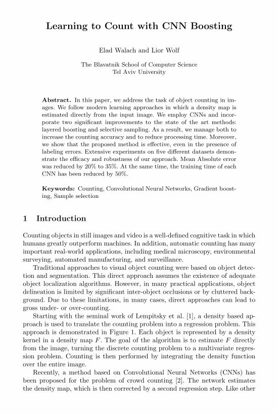
Starting with the seminal work of Lempitsky et al. [1], a density based ap-proach is used to translate the counting problem into a regression problem. Thisapproach is demonstrated in Figure 1. Each object is represented by a densitykernel in a density map F . The goal of the algorithm is to estimate F directlyfrom the image, turning the discrete counting problem to a multivariate regres-sion problem. Counting is then performed by integrating the density functionover the entire image.

Recently, a method based on Convolutional Neural Networks (CNNs) hasbeen proposed for the problem of crowd counting [2]. The network estimatesthe density map, which is then corrected by a second regression step. Like other

2 Walach and Wolf

Fig. 1. Examples of density maps. (a) A synthetic fluorescence-light microscopy im-age [1] (left) and corresponding label density map (right). (b) A perspective normalizedcrowd image from the UCSD dataset [3] (left) and corresponding label density map(right). In both applications, machine learning techniques are used to estimate theappropriate density map values for each pixel. (c) The kernel used to create the mi-croscopy density map. (d) The kernel used to create the crowd density map.

CNN based methods, this approach allows end-to-end training without the needto design any hand crafted image features and yields state of the art results asdemonstrated on current object counting benchmarks: USCD [3] and UCF [4].

In this work, we adopt the CNN approach and introduce several novel mod-ifications, which yield a significant improvement both in accuracy and perfor-mance. One such modification is in the boosting process. We propose a layeredapproach, where training is done in stages. We iteratively add CNNs, so thatevery new CNN is trained to estimate the residual error of the earlier prediction.After the first CNN is trained, the second CNN is trained on the difference be-tween the estimation and the ground truth. The process then continues to thethird CNN and so on.

Our second contribution is an intuitive yet powerful sample selection algo-rithm that yields both higher accuracy and faster training times. The idea is tostreamline the training process by reducing the impact of the low quality sam-ples, such as trivial cases or outliers. We propose to use the error of each sampleas a measure of its quality. Our assumption is that very low errors indicate trivialcases. Conversely, very high errors indicate outliers. Accordingly, for a number oftraining epochs, we mute both low and high error samples. Reducing the impactof outliers is instrumental in increasing the overall accuracy of the method. Atthe same time, an effective decrease in the overall number of training samplesreduces the training time of each CNN in the boosted ensemble.

It should be noted that layered boosting and selective sampling complementeach other. Boosting increases the overall number of trained network layers,which drives up the training time. Boosting also leads to an over emphasis ofmisclassified samples such as outliers. Selective sampling mitigates both theseundesirable effects.

Learning to Count with CNN Boosting 3

2 Previous work

The straightforward approach to counting is based on counting objects detectedby an image segmentation process, see, for example, [5, 6]. However, such meth-ods are limited by the accuracy of the underlying detection methods. Accord-ingly, direct approaches tend to have difficulties in handling severe occlusionsand cluttered backgrounds.

A direct machine learning approach was suggested in [7–9], which estimatesthe number of objects based on a predetermined set of image features such as im-age histograms. Naturally, the use of 1D statistics leads to a great computationalefficiency. However, these global approaches tend to disregard 2D information onthe object location. As a result, in some complex counting applications, accuracymay be affected.

Lempitsky et al. [1] introduced an object counting method that is based onpixel-level object density map regression. The method was shown to performwell, even in the face of a high number of objects that occlude each other.Following this work, Fiaschi et al. [10] used random forest regression in orderto estimate the object density and improve training efficiency. Pham et al. [11]suggested additional improvements using modified random forests.

Deep learning is often used for tasks that are related to crowd countingsuch as pedestrian detection [12, 13] and crowd segmentation [14]. Two recentcontributions [2, 15] have used deep models specifically for the application ofcrowd counting. In [2], a dual-loss function was suggested for the estimation ofboth the density function and the crowd count simultaneously. In [15], a methodwas proposed for counting extremely dense crowds using a CNN. In this work,the step of estimating the density function was not performed. Instead, the CNNdirectly estimated the number of people in the crowd. In addition, the utility ofaugmenting the training data with negative samples (no people) was explored.

In contrast to other methods, our approach proposes to estimate the den-sity map directly with a single loss function. In order to mitigate the difficultyof training deep regression networks, we propose the use of relatively shallownetworks augmented by the boosting framework.

Boosting deep networks Boosting is a well-known greedy technique for ensemblelearning. The basic idea is to literately train a new classifier that learns tofix the errors of the previous classifiers. In general, boosting is most powerfulwhen used to combine weak models, and boosting stronger models is often notbeneficial [16]. Specifically, only a few attempts have been made for boostingdeep neural networks.

In [17], a hybrid method based on boosting is proposed. First, object can-didates are determined based on low-level features extracted from the bottomlayers of a trained CNN. AdaBoost [18] is then used to build a final classifier.

In this paper, we employ boosting in a straightforward manner, workingiteratively with the same network. The method is general and the same networkarchitecture is used for all the applications. Despite the simplicity of the proposedapproach, it yields excellent results.

4 Walach and Wolf

Sample Selection: Training deep networks is often done by utilizing very largedatasets. Many methods have been proposed for data augmentation in order toincrease the training set size even further. However, not all training samples arecreated equal. For instance, [19] proposed a sample selection scheme to choosethe best samples within a sample augmentation framework. For each trainingsample, a continuous stream of augmented samples is created. Then, in betweenepochs, the network evaluates the error of each of the synthesized samples. Onlyhigh error samples are retained to form the final training set.

Sample selection is often used as a part of cascaded architectures. Cascadeshave been used, e.g., for face detection using either hand crafted features [20], ordeep learning [21]. When constructing the next level of the cascade, the samplesthat did not pass the previous classifiers are filtered out.

Another commonly used method is the one of harvesting hard negative sam-ples, which is used for face detection and for object detection in general, e.g.see [22]. Recently, in the domain of face recognition [23], it has been proposed toconstruct a dataset of individuals that are similar to each other and are thereforeharder to identify. The face recognition network is then fine-tuned on this morechallenging sample set.

3 Density counting with CNNs

Following previous work, we define the density function as a real-valued functionover the pixel grid, such that its integral over the image domain matches theobject counts. The input to our method is a single image I, and, during training,a set S of image locations that correspond to the centers of the objects to becounted. The density map F is the image obtained by placing a 2D kernel P ateach location p ∈ S:

F (x) =∑p∈S

P (x− p) , (1)

where x denotes 2D image coordinates. For the microscopy dataset, we follow [1]and employ P that is a normalized 2D Gaussian kernel. For the crowd-countingexperiment, we follow [2] and use a specific smoothing kernel designed for thistask. This filter is a human-shaped structure composed as a superposition of twoGaussians, one for the head and one for the body. In Figure 1, examples of groundtruth density maps are presented for both microscopy and crowd counting, aswell as the kernels used.

Counting in the density map domain is done by spatial integration. It isimportant to note, however, that using the definition above, the sum of theground truth density F over the entire image will not match the object countexactly. This effect is caused by objects that lie very close to the image boundaryso that part of the associated probability mass is located outside of the image.However, for most applications, this effect can be neglected.

Any regression algorithm can be used for counting within such a framework.The objective of the regression model is to learn the mapping from the imagepixels to the density map of the image. In our deep learning method, similar


(a)

(b)

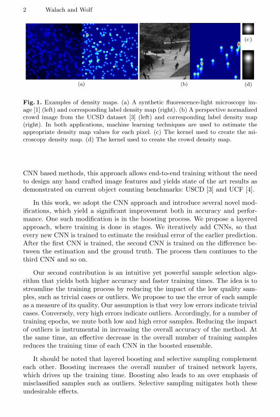
Fig. 2. The proposed CNN architecture. The basic network architecture is composedof 3 blocks. The first two blocks contain convolutional layers followed by max-pooling.The final block is composed of a single convolutional layer (for crowd) and a seriesof fully connected layers without pooling. (a) The cell counting problem. We use 2convolutional blocks. Each block consists of 3x3 convolution layers, ending with 2x2pooling and dropout. After the two convolutional blocks, we add a fully connected layerwith 100 neurons. (b) The crowd counting problem. There are two 7x7 convolutions,each followed by 2x2 pooling. Finally, a 5x5 convolution layer followed by two fullyconnected layers are added.

to [2], a CNN is used in order to map an image patch to the correspondingpatch of the density image.

Patches randomly selected from the training images are treated as trainingsamples, and the corresponding patches of the density map form the labels.As with other density based methods, counting is performed by summing theestimated density map. Note that unlike [2], we do not use the density map asa feature for a second regression model. Instead, we directly integrate over thedensity map. We have used two slightly different CNN architectures to addressthe two counting problems. In both cases, the input consists of patches of theinput image I, and the output is an estimated density map for each patch.The CNN architecture for microscopy counting can be seen in Figure 2(a), andthe one used for crowd counting is depicted in Figure 2(b). The differences aremainly in the size of the input patch, which, in turn, is determined by the size ofthe objects to be counted. In both cases, the architecture is built out of severalconvolutional blocks, which contain interleaving 2x2 pooling layers. After eachconvolutional block, we add a dropout layer [24], with a parameter 0.5. Thefinal block is composed of a single convolutional layer (for crowd) and a series of

6 Walach and Wolf

fully connected layers without pooling. After each layer, except for the topmosthidden layer, we employ a ReLU activation function [25].

Since we use two 2x2 pooling layers, the output density patch is 1/4 the sizeof the original patch, in each dimension. We use the Euclidean (L2) distance asthe loss function. This is in contrast to [2], which employs a dual regression lossfunction in order to overcome the relatively more challenging training of regres-sion problems. In our case, we train using RMSProp [26] instead of StochasticGradient Descent and are able to train even without modifying the loss function.Weights were initialized using the Xavier-improved method [27].

At test time, patches are extracted from the test image using a sliding windowapproach. We adjust the stride such that there is a 50% overlap. The densityestimation of each pixel in the output image is obtained by averaging all thepredictions of the overlapping patches that contain the given pixel. The finalobject count in the image is then obtained by summing all values of the recovereddensity map.

4 Gradient boosting of CNNs

Gradient boosting machines belong to a family of powerful machine-learningensemble techniques that have shown considerable success in a wide range ofpractical applications. Common ensemble techniques, such as random forests,rely on simple averaging of models in the ensemble. Boosting methods, includinggradient boosting, are based on a different, constructive strategy for the ensembleformation. There, new models are added to the ensemble sequentially. At eachiteration, a new base-learner model fn is trained to fix the errors of the previousensemble Fn−1

fn(x) = arg minfn(x)

Ex[

expected loss for one sample︷︸︸︷Ey(Ψ [y, fn + Fn−1(x)]) |x]︸︷︷︸

expectation over the entire dataset

, (2)

where fn(x) is the n-th base-learner, Ψ is the loss function and Fn−1 =∑n−1

1 fi.One can consider several different strategies for boosting, i.e. different ways

to find the error-minimizing function. A well-known formulation is that of thegradient-descent method, which is called gradient boosting machines or GBMs [28,29]. The principle idea is to construct the next learner fn to be maximally cor-related with the negative gradient of the loss function of the current ensembleFn−1. Therefore, this method follows gradient descent in the function space.

For the Euclidean loss, this amounts to a simple strategy of fitting a model tothe current error. In our case, in each step, we fit a new CNN model fn = CNNn

to the error of the last round F (x)−Fn−1 and update the ensemble accordingly

Fn ← Fn−1 + CNNn(θ) (3)

An overview of our boosting mechanism is presented in Figure 3. The validation


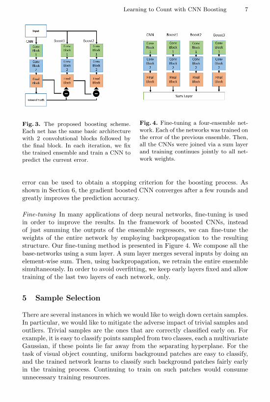
Fig. 3. The proposed boosting scheme.Each net has the same basic architecturewith 2 convolutional blocks followed bythe final block. In each iteration, we fixthe trained ensemble and train a CNN topredict the current error.

Fig. 4. Fine-tuning a four-ensemble net-work. Each of the networks was trained onthe error of the previous ensemble. Then,all the CNNs were joined via a sum layerand training continues jointly to all net-work weights.

error can be used to obtain a stopping criterion for the boosting process. Asshown in Section 6, the gradient boosted CNN converges after a few rounds andgreatly improves the prediction accuracy.

Fine-tuning In many applications of deep neural networks, fine-tuning is usedin order to improve the results. In the framework of boosted CNNs, insteadof just summing the outputs of the ensemble regressors, we can fine-tune theweights of the entire network by employing backpropagation to the resultingstructure. Our fine-tuning method is presented in Figure 4. We compose all thebase-networks using a sum layer. A sum layer merges several inputs by doing anelement-wise sum. Then, using backpropagation, we retrain the entire ensemblesimultaneously. In order to avoid overfitting, we keep early layers fixed and allowtraining of the last two layers of each network, only.

5 Sample Selection

There are several instances in which we would like to weigh down certain samples.In particular, we would like to mitigate the adverse impact of trivial samples andoutliers. Trivial samples are the ones that are correctly classified early on. Forexample, it is easy to classify points sampled from two classes, each a multivariateGaussian, if these points lie far away from the separating hyperplane. For thetask of visual object counting, uniform background patches are easy to classify,and the trained network learns to classify such background patches fairly earlyin the training process. Continuing to train on such patches would consumeunnecessary training resources.

8 Walach and Wolf

Algorithm 1 The sample selection scheme.

∀s ∈ allSamples:Sleep[s]← 0

for each training epoch doactiveSamples← {s|sampleSleep[s] = 0}∀s ∈ allSamples , Sleep[s]← max(0, Sleep[s]− 1)net← processEpoch(net, activeSamples)∀s ∈ activeSamples , Err(s)← loss (net, s)Θlow ← percentile(Err, activeSamples, 30)Θhigh ← percentile(Err, activeSamples, 97)badSamples← {s ∈ activeSamples|Err[s] < Θlow ∨ Err[s] > Θhigh}∀s ∈ badSamples , Sleep[s]← 4

end for

Another source of training inefficiency is due to the presence of outliers. Inmany practical applications, outliers are caused by the mislabeled samples. Sucherrors in the input data are clearly detrimental to the classifier’s efficacy. Indeed,it was shown that some boosting algorithms including AdaBoost are extremelysensitive to outliers [30].

Accordingly, we propose to reduce the impact of low quality training samplesby decreasing their participation in the training process. This raises the questionof identifying the low quality samples described above. In our method, we employthe current error of each individual training sample as a measure of the sample’squality. A very low L2 distance between the estimated and true target, indicatesa trivial sample, while a high error indicates an outlier. Therefore, samples witheither high or low errors are deemed to be of low quality.

After each epoch, we continue to train only on the samples with an errorrate between Θlow and Θhigh, where Θlow and Θhigh are thresholds chosen as acertain percentiles of the errors of the entire training set. Based on initial crossvalidation tests performed on 20% of the training data of the UCSD dataset, weset Θhigh to be the 97 percentile and Θlow as the 30 percentile throughout ourexperiments. The examples that did not meet the threshold criteria are removedfrom the training process for several epochs. Specifically, in our experiments, alow quality sample “sleeps” for four epochs. Algorithm 1 shows our proposedsample selection scheme.

One can think of other sample selection schemes. For instance, anotherscheme could be weighting each sample’s gradients according to its error. How-ever, a temporal elimination of a sample has clear advantages in terms of thetraining time, since irrelevant training samples are completely removed and notjust weighted down.

Note that for the above mentioned parameters, at each epoch, 33% of theactive samples are removed. Viewed as a timed process in which the numberof active samples converge, we obtain that at each round the same number ofsamples are removed. Let N be the total number of training samples. At thesteady state, the following equation holds: N = x + 4 × 0.33 × x, where x is


the number of active samples. Therefore, the number of active training samplesconverges to x ≈ 0.43N . In other words, at any given epoch, after an initialnumber of epochs, only about 43% of all the samples actively participate in thetraining process.

Our sample selection approach is simple and straightforward. Nevertheless,as demonstrated in the experiments below, it yields a significant improvementboth in terms of training time and, especially for noisy labeled data, also interms of accuracy.

6 Experiments

We compare our algorithm to the state of the art in two domains: Bacterial cellimages and crowd counting. Overall, our experiments are more extensive thanany previous counting paper. The only dataset that seems to be missing is theExpo crowd dataset [2], which is not publicly available. Additional experimentsholding out 5% of the tagging are done in order to demonstrate the method’srobustness to outliers. Finally, we present surprising results for depth estimationfrom a single image, which are obtained using the same network we propose forthe completely different task of crowd counting.

6.1 Bacterial cells microscopy images

The dataset presented in [1] is composed out of 200 simulated fluorescence mi-croscopy images of cell cultures, each containing 171 ± 64 cells on average. 100images are reserved for training and validation, and the remaining 100 for test-ing. Each image has a labeled equivalent with dots marked at the center of eachcell. The label density map was calculated by smoothing this point density mapusing a Gaussian kernel with σ = 3 pixels.

Following [10], we discard the green and red channels of the raw images anduse only the blue channel. From each training image, we take 1600 random 32×32patches. Our CNN architecture is the one presented in Figure 2(a).

The results are summarized in Table 1. As in other counting benchmarks, themean absolute error (MAE) is used for evaluating the accuracy of each method.As can be seen, for the given data set, without boosting, the single networkdoes not achieve good results. However, with the increase in the number ofboosting stages, MAE is reduced yielding a significant (more than 30 percent)improvement over the state of the art results. While the improvement in accuracyfollowing the booting rounds is significant, it seems that more than four rounds(five networks) are not necessary and even detrimental. This is probably due tooverfitting the remaining error. On this very small dataset of 100 images, wecould not improve results using fine-tuning.

The boosted classifier, which consists of multiple networks, has increasedcapacity. Therefore, we perform additional experiments in order to rule out thepossibility that the increased performance is simply due to the increase in thecapacity. For this purpose, we have added more convolutional layers creating

10 Walach and Wolf

MAEMethod Test

Detection+correction [1] 4.9Density+MESA [1] 3.5Regression trees [10] 3.2

Ensemble of 2 CNNs 6.71Ensemble of 3 CNNs 6.54Ensemble of 4 CNNs 6.42Ensemble of 5 CNNs 6.45Ensemble of 6 CNNs 6.44Ensemble of 7 CNNs 6.43

MAE MAE NoMethod Test Validation Selection

Our model (no boosting) 6.82 8.59 6.93Boosted CNN (1 boost) 3.20 3.46 3.42Boosted CNN (2 boosts) 2.81 3.00 2.71Boosted CNN (3 boosts) 2.42 2.50 2.39Boosted CNN (4 boosts) 2.19 2.16 2.21Boosted CNN (5 boosts) 2.33 2.18 2.41Fine-tuned (4 boosts) 2.19 2.16 2.22

CNN twice as deep 5.40 5.62 5.22CNN three times as deep 16.42 17.39 14.68

Table 1. MAE on the microscopy dataset. We present literature results as well asresults for our boosted network, following 1–6 rounds of boosting. Deeper networks(without boosting) and ensemble of multiple CNNs are also shown. In our terminology,1 boost means two networks. For completeness, we also present (rightmost column)MAE on the test set without sample selection.

networks twice and three times as deep. The results show that a network twiceas deep is better than the shallow network we use for boosting. However, boostingsignificantly outperforms increase in the network depth. The network three timesas deep is much worse than even the shallow network, probably due to overfittingand the difficulty of training very deep networks.

It is well known that one can improve results by creating an ensemble ofCNNs trained from different random starting points. Hence, we have performeda second experiment applying this technique. The same CNN, as the one uti-lized for boosting, is used for the ensemble experiments. Clearly, the boostingapproach outperforms that of ensemble averaging.

6.2 Crowd counting benchmarks

The UCSD dataset [3] is comprised of a 2000-frame video chosen from onesurveillance camera on the UCSD campus. The video in this dataset was recordedat 10 fps with a frame size of 158×238. The labeled ground truth is at the centerof every pedestrian. The ROI and perspective map are provided in the dataset.We follow the setup of [2], and perform perspective normalization such that aground area of 3-meters by 3-meters is mapped to a 48 pixel by 48 pixel region.

The benchmark sets aside frames 601-1400 as the training data and the re-maining 1200 frames as the test set. For training, we extract 800 48×48 randompatches from each training image.

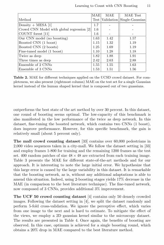
Unlike some density map models that use regression on the density map [2] asa post-processing step, our estimated count is the direct integral over the densitymap. Comparison with other methods performing crowd counting on the UCSDdataset is presented in the Table 2. Once again, the MAE metric is employedfor the accuracy evaluation. As can be seen, the proposed boosted CNN model


MAE MAE MAE TestMethod Test Validation Single-Gaussian

Density + MESA [1] 1.7 - -Crowd CNN Model with global regression [2] 1.6 - -COUNT forest [11] 1.6 - -

Our CNN model (no boosting) 1.63 1.42 1.57Boosted CNN (1 boost) 1.15 1.32 1.19Boosted CNN (2 boosts) 1.25 1.69 1.19Fine-tuned model (1 boost) 1.10 1.28 1.18

Twice as deep 1.82 1.88 1.91Three times as deep 2.42 2.63 2.88

Ensemble of 2 CNNs 1.55 1.55 1.63Ensemble of 3 CNNs 1.53 1.51 1.56

Table 2. MAE for different techniques applied on the UCSD crowd dataset. For com-pleteness, we also present (rightmost column) MAE on the test set for a single Gaussiankernel instead of the human shaped kernel that is composed out of two guassians.

outperforms the best state of the art method by over 30 percent. In this dataset,one round of boosting seems optimal. The low-capacity of this benchmark isalso manifested in the low performance of the twice as deep network. In thisdataset, fine-tuning the boosted network, which contains two CNNs (1 boost),does improve performance. However, for this specific benchmark, the gain isrelatively small (about 5 percent only).

The mall crowd counting dataset [33] contains over 60,000 pedestrians in2,000 video sequences taken in a city-mall. We follow the dataset setting in [33]and employ frames 1-800 for training and the remaining 1200 frames as the testset. 400 random patches of size 48× 48 are extracted from each training image.Table 3 presents the MAE for different state-of-the-art methods and for ourapproach. It is interesting to note the large initial error. We hypothesize thatthis large error is caused by the large variability in this dataset. It is remarkablethat the boosting network, as is, without any additional adaptations is able toamend this situation. Indeed, using 2-boosting stages yields 17% decrease in theMAE (in comparison to the best literature technique). The fine-tuned network,now composed of 3 CNNs, provides additional 3% improvement.

The UCF 50 crowd counting dataset [4] contains only 50 densely crowdedimages. Following the dataset setting in [4], we split the dataset randomly andperform 5-fold cross-validation. We ignore the perceptive effect, which variesfrom one image to the next and is hard to estimate. To mitigate the effect ofthe views, we employ a 2D gaussian kernel similar to the microscopy dataset.The results are presented in Table 4. Once again, the benefits of boosting areobserved. In this case, optimum is achieved for a single boosting round, whichobtains a 20% drop in MAE compared to the best literature method.

12 Walach and Wolf

MAE MAE va-Method Test lidation

CA-RR [31] 3.43 -COUNT forest [11] 2.50 -

One CNN 9.54 8.51Boosted CNN (1 boost) 2.43 3.19Boosted CNN (2 boosts) 2.08 2.31Boosted CNN (3 boosts) 2.13 2.78Fine-tuned (2 boosts) 2.01 2.25

Twice as deep 10.41 11.24Three times as deep 15.37 14.42

Ensemble of 2 CNNs 6.52 7.21Ensemble of 3 CNNs 6.67 7.19

Table 3. MAE for different techniquesapplied on the mall crowd-countingdataset.

MAE MAE va-Method Test lidation

Density+MESA [1] 493.4 -Idrees et al. [4] 468.0 -Zhang et al. [2] 467.0 -

One CNN (no boost) 434.4 452.4Boosted (1 boost) 376.2 425.2Boosted (2 boosts) 382.2 560.3Find-tuned (1 boost) 364.4 341.4

Twice as deep 539.2 500.3Three times as deep 914.2 712.8

Ensemble of 2 CNNs 414.2 553.2Ensemble of 3 CNNs 474.0 680.5

Table 4. MAE for different techniquesapplied on the UCF crowd-countingdataset.

BoostNo

selectionWith

selectionThe selection

proposed in [32]

none 18.80 14.55 15.721 10.09 7.88 8.182 8.12 6.25 6.323 8.49 4.94 5.124 9.12 4.96 5.42

Table 5. Impact of the sample selectionon the MAE when 5% of the cells arerandomly untagged in the cell microscopybenchmark.

BoostNo

selectionWith

selectionThe selection

proposed in [32]

none 9.03 7.82 11.391 6.92 2.97 4.442 5.49 2.52 2.463 3.76 2.25 2.484 4.01 2.64 2.81

Table 6. Impact of the sample selectionprocess on the MAE when a random subsetcontaining 5% of the people in the malldataset are untagged.

6.3 Robustness to outliers

The sample selection process has a dramatic effect on the training time, since, atthe steady state, only 43% of samples are used at each epoch, while the amountof epochs stays the same. However, its effect on accuracy is more limited. Table 1shows MAE, for the cell counting dataset, with and without sample selection.Asone can see, the effect on accuracy is small. For example, with four boostingsteps, sample selection reduces MAE from 2.21 to 2.19.

However, as shown below, in more ambiguous tagging situations, or in caseswhere tagging is inaccurate, sample selection becomes crucial. In order to sim-ulate this effect, we randomly removed 5% of points from the set S of the trueobject locations for the training samples.

The results are summarized in Table 5 for the cell counting benchmark andTable 6 for the mall crowd counting dataset. It is interesting to see that even


(a) (b) (c) (d)

Fig. 5. Examples of Make3D [34] depth maps. (a) a test image. (b) estimation with asingle CNN. (c) estimation after 1 additional round of boosting. (d) ground truth.

RMS(m) RMS(m)Method Test Validation

Depth MRF [34] 16.7 -Feedback Cascades [35] 15.2 -Depth Transfer [36] 15.10 -DCNF [37] 12.89 -Discrete-continuous CRF [38] 12.60 -

Our CNN model (no boosting) 14.36 13.69Boosted CNN (1 boost) 13.69 13.31Boosted CNN (2 boosts) 13.61 12.57Boosted CNN (3 boosts) 13.89 13.12Fine-tuned model (2 boosts) 13.28 12.52

Table 7. Results on thedepth estimation Make3Ddataset [34]. We presentliterature results as wellas results for our boostednetwork.

a very limited 5% corruption in the ground truth causes a very significant (upto 3-fold ) increase in the MAE. However, introduction of the selective samplingmethod allows over 40 percent error rate reduction (4.94 instead of 8.49 for threeboosting steps in the cell dataset).

It is interesting to note that, in the mall dataset, our method applied on thenoisy ground truth data achieves better accuracy than the best literature resultobtained on the uncorrupted truth set (2.25 compared to 2.50).

In addition, we evaluated the sample selection scheme proposed in [32], whichemploys a robust loss function based on Tukeys biweight function that weighsthe training samples based on the residual magnitude. As can be seen in tables5 and 6, our method yields lower error than state of the art.

6.4 Depth estimation

Since the proposed boosting method, at the core of our method, is general, it canbe applied outside the realm of object counting. There are many image to imageregression problems with a similar structure to the density estimation task. Wearbitrarily select the problem of depth estimation from a single image.

The Make3D range image dataset [34, 39] is used in the following depth es-timation experiments. Each image in this dataset is of size 2272x1704 and issupplied with a 55x305 depth map. We adhere to the benchmark splits providedin [37], which consist of 400 training images and 134 test images.

14 Walach and Wolf

For training, we resize the images by half and sample 800 112× 112 patches.We use the same CNN architecture as the crowd counting(!). The only differenceis the number of neurons in the final fully-connected layers. Since the last layerrepresents the estimated depth for a patch of size 28× 28 pixels the final fully-connected layers contain 1000 and then 784 neurons instead of the original sizesof 400 and 200. The ground truth depth data of Make3D is inaccurate for depthsgreater than 80m. Therefore, we follow the commonly applied post-processingdescribed in [38] that classifies sky pixels and sets their depth to 80m.

The results on the Make3D benchmark are evaluated using the RMS (rootmean-squared) measure. Tab. 7 presents our boosting results in comparison tothe literature, and Fig. 5 shows an example. The only literature methods, weare aware of, that outperform us are the Discrete-continuous CRF [38] and Deepconvolutional neural fields [37]. Note that our method is local and does not useCRF models as the other leading methods do. The application of our method isdirect, and does not include the common practice of working with superpixels.Nevertheless, our simplified approach is within 5.5% of the state of the art.

7 Conclusions and future work

In this work, we propose two contributions that improve the effectiveness ofCNNs: gradient boosting and selective sampling. The efficacy of these techniqueswas evaluated in the domain of visual object counting. We applied the techniqueson four public benchmarks and showed that our approach yields a 20%-30%reduction in the counting error rate. When training the CNNs, we are able toobtain more than 50% reduction in training time of each CNN.

An additional advantage of the proposed approach is its simplicity. We areusing the same basic architecture for three different counting applications (mi-croscopy, indoor and outdoor crowd) and achieve improved results in comparisonto the state-of-the-art methods tuned to each specific application. Interestingly,in all the cases we had a similar degree of accuracy improvement over the liter-ature, even though each benchmark has its own leading method.

In this paper, we explored the basic premise of the above methods. However,there are several improvements that we would like to explore in the future. Theseinclude an adaptive parameterization for the sample selection parameters: highand low thresholds and number of muted epochs. This can be based, for example,on the relative contribution of each sample to the weight updates.

Finally, it is our intention to extend the proposed techniques to more CNNregression applications. Such problems exist in a variety of domains includingtasks that differ significantly from the task of counting such as age estimationin face images and human pose estimation.

Acknowledgments

This research is supported by the Intel Collaborative Research Institute for Com-putational Intelligence (ICRI-CI).


References

1. Lempitsky, V., Zisserman, A.: Learning to count objects in images. In Lafferty,J.D., Williams, C.K.I., Shawe-Taylor, J., Zemel, R.S., Culotta, A., eds.: Advancesin Neural Information Processing Systems 23. Curran Associates, Inc. (2010) 1324–1332

2. Zhang, C., Li, H., Wang, X., Yang, X.: Cross-scene crowd counting via deepconvolutional neural networks. In: The IEEE Conference on Computer Vision andPattern Recognition (CVPR). (June 2015)

3. Chan, A.B., sheng John, Z., Vasconcelos, L.N.: Privacy preserving crowd monitor-ing: Counting people without people models or tracking. CVPR (2008) 1–7

4. Idrees, H., Saleemi, I., Seibert, C., Shah, M.: Multi-source multi-scale countingin extremely dense crowd images. In: Proceedings of the 2013 IEEE Conferenceon Computer Vision and Pattern Recognition. CVPR ’13, Washington, DC, USA,IEEE Computer Society (2013) 2547–2554

5. Dong, L., Parameswaran, V., Ramesh, V., Zoghlami, I.: Fast crowd segmenta-tion using shape indexing. In: Computer Vision, 2007. ICCV 2007. IEEE 11thInternational Conference on. (Oct 2007) 1–8

6. An, S., Peursum, P., Liu, W., Venkatesh, S.: Efficient algorithms for subwindowsearch in object detection and localization. In: Computer Vision and PatternRecognition, 2009. CVPR 2009. IEEE Conference on. (June 2009) 264–271

7. Ryan, D., Denman, S., Fookes, C., Sridharan, S.: Crowd counting using multiplelocal features. In: Digital Image Computing: Techniques and Applications, 2009.DICTA ’09. (Dec 2009) 81–88

8. Idrees, H., Saleemi, I., Seibert, C., Shah, M.: Multi-source multi-scale countingin extremely dense crowd images. In: Proceedings of the 2013 IEEE Conferenceon Computer Vision and Pattern Recognition. CVPR ’13, Washington, DC, USA,IEEE Computer Society (2013) 2547–2554

9. Chan, A.B., Liang, Z.S.J., Vasconcelos, N.: Privacy preserving crowd monitoring:Counting people without people models or tracking. In: Computer Vision andPattern Recognition, 2008. CVPR 2008. IEEE Conference on. (June 2008) 1–7

10. Fiaschi, L., Koethe, U., Nair, R., Hamprecht, F.A.: Learning to count with re-gression forest and structured labels. In: Pattern Recognition (ICPR), 2012 21stInternational Conference on. (Nov 2012) 2685–2688

11. Pham, V.Q., Kozakaya, T., Yamaguchi, O., Okada, R.: Count forest: Co-votinguncertain number of targets using random forest for crowd density estimation. In:The IEEE International Conference on Computer Vision (ICCV). (December 2015)

12. Zeng, X., Ouyang, W., Wang, M., Wang, X.: Deep Learning of Scene-SpecificClassifier for Pedestrian Detection. In: Computer Vision – ECCV 2014: 13th Eu-ropean Conference, Zurich, Switzerland, September 6-12, 2014, Proceedings, PartIII. Springer International Publishing, Cham (2014) 472–487

13. Zeng, X., Ouyang, W., Wang, X.: Multi-stage contextual deep learning for pedes-trian detection. In: Computer Vision (ICCV), 2013 IEEE International Conferenceon. (Dec 2013) 121–128

14. Kang, K., Wang, X.: Fully convolutional neural networks for crowd segmentation.CoRR abs/1411.4464 (2014)

15. Wang, C., Zhang, H., Yang, L., Liu, S., Cao, X.: Deep people counting in ex-tremely dense crowds. In: Proceedings of the 23rd ACM International Conferenceon Multimedia. MM ’15, New York, NY, USA, ACM (2015) 1299–1302

16 Walach and Wolf

16. Li, X., Wang, L., Sung, E.: A study of adaboost with svm based weak learners. In:Neural Networks, 2005. IJCNN ’05. Proceedings. 2005 IEEE International JointConference on. Volume 1. (July 2005) 196–201 vol. 1

17. Karianakis, N., Fuchs, T.J., Soatto, S.: Boosting convolutional features for robustobject proposals. CoRR abs/1503.06350 (2015)

18. Freund, Y., Schapire, R.E.: A decision-theoretic generalization of on-line learningand an application to boosting (1997)

19. Takayoshi Yamashita1, Taro Watasue, Y.Y., Fujiyoshi, H.: Improving quality oftraining samples through exhaustless generation and effective selection for deepconvolutional neural networks. (ICPR (2012)

20. Viola, P., Jones, M.: Rapid object detection using a boosted cascade of simplefeatures. In: Computer Vision and Pattern Recognition, 2001. CVPR 2001. Pro-ceedings of the 2001 IEEE Computer Society Conference on. Volume 1., IEEE(2001) I–511

21. Li, H., Lin, Z., Shen, X., Brandt, J., Hua, G.: A convolutional neural networkcascade for face detection. In: Proceedings of the IEEE Conference on ComputerVision and Pattern Recognition. (2015) 5325–5334

22. Sung, K.K., Poggio, T.: Example-based learning for view-based human face detec-tion. IEEE Trans. Pattern Anal. Mach. Intell. 20(1) (January 1998) 39–51

23. Taigman, Y., Yang, M., Ranzato, M., Wolf, L.: Web-scale training for face identi-fication. CoRR abs/1406.5266 (2014)

24. Srivastava, N., Hinton, G., Krizhevsky, A., Sutskever, I., Salakhutdinov, R.:Dropout: A simple way to prevent neural networks from overfitting. Journal ofMachine Learning Research 15 (2014) 1929–1958

25. Glorot, X., Bordes, A., Bengio, Y.: Deep sparse rectifier neural networks. InGordon, G.J., Dunson, D.B., eds.: Proceedings of the Fourteenth InternationalConference on Artificial Intelligence and Statistics (AISTATS-11). Volume 15.,Journal of Machine Learning Research - Workshop and Conference Proceedings(2011) 315–323

26. Tieleman, T., Hinton, G.: Lecture 6.5—RmsProp: Divide the gradient by a run-ning average of its recent magnitude. COURSERA: Neural Networks for MachineLearning (2012)

27. He, K., Zhang, X., Ren, S., Sun, J.: Delving deep into rectifiers: Surpassing human-level performance on imagenet classification. CoRR abs/1502.01852 (2015)

28. Friedman, J.H.: Greedy function approximation: A gradient boosting machine.Annals of Statistics 29 (2000) 1189–1232

29. Friedman, J.H.: Stochastic gradient boosting. Comput. Stat. Data Anal. 38(4)(February 2002) 367–378

30. Long, P.M., Servedio, R.A.: Random classification noise defeats all convex potentialboosters. Machine Learning 78(3) (2009) 287–304

31. Chen, K., Gong, S., Xiang, T., Loy, C.C.: Cumulative attribute space for age andcrowd density estimation. In: Computer Vision and Pattern Recognition (CVPR),2013 IEEE Conference on. (June 2013) 2467–2474

32. Belagiannis, V., Rupprecht, C., Carneiro, G., Navab, N.: Robust optimization fordeep regression. CoRR abs/1505.06606 (2015)

33. Chen, K., Loy, C.C., Gong, S., Xiang, T.: Feature mining for localised crowdcounting. In: In BMVC

34. Saxena, A., Chung, S.H., Ng, A.Y.: Learning depth from single monocular images.In: In NIPS 18, MIT Press (2005)


35. Li, C., Kowdle, A., Saxena, A., Chen, T.: Towards holistic scene understand-ing: Feedback enabled cascaded classification models. In Lafferty, J.D., Williams,C.K.I., Shawe-Taylor, J., Zemel, R.S., Culotta, A., eds.: Advances in Neural Infor-mation Processing Systems 23. Curran Associates, Inc. (2010) 1351–1359

36. Karsch, K., Liu, C., Kang, S.B.: Depth extraction from video using non-parametricsampling. In: Proceedings of the 12th European Conference on Computer Vision- Volume Part V. ECCV’12, Berlin, Heidelberg, Springer-Verlag (2012) 775–788

37. Liu, F., Shen, C., Lin, G., Reid, I.D.: Learning depth from single monocular imagesusing deep convolutional neural fields. CoRR abs/1502.07411 (2015)

38. Liu, M., Salzmann, M., He, X.: Discrete-continuous depth estimation from a singleimage. In: The IEEE Conference on Computer Vision and Pattern Recognition(CVPR). (June 2014)

39. Saxena, A., Sun, M., Ng, A.Y.: Make3d: Learning 3d scene structure from a singlestill image. IEEE Trans. Pattern Anal. Mach. Intell. 31(5) (May 2009) 824–840

learning to count with cnn boosting - ביה"ס למדעי...

Documents