least-squares regressiondewan.buet.ac.bd/eee423/coursematerials/curve-fitting.pdf · are met,...

17C H A P T E R 17

454

Least-Squares Regression

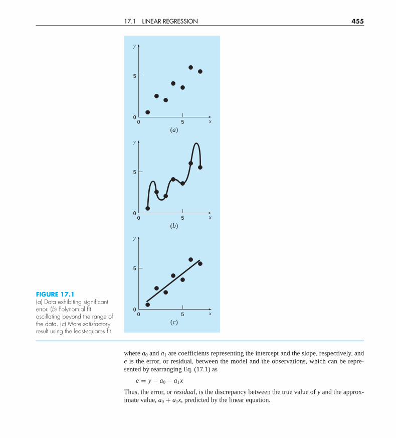
Where substantial error is associated with data, polynomial interpolation is inappropriateand may yield unsatisfactory results when used to predict intermediate values. Experimen-tal data is often of this type. For example, Fig. 17.1a shows seven experimentally deriveddata points exhibiting significant variability. Visual inspection of the data suggests a posi-tive relationship between y and x. That is, the overall trend indicates that higher values of yare associated with higher values of x. Now, if a sixth-order interpolating polynomial is fit-ted to this data (Fig. 17.1b), it will pass exactly through all of the points. However, becauseof the variability in the data, the curve oscillates widely in the interval between the points.In particular, the interpolated values at x = 1.5 and x = 6.5 appear to be well beyond therange suggested by the data.

A more appropriate strategy for such cases is to derive an approximating function thatfits the shape or general trend of the data without necessarily matching the individualpoints. Figure 17.1c illustrates how a straight line can be used to generally characterize thetrend of the data without passing through any particular point.

One way to determine the line in Fig. 17.1c is to visually inspect the plotted data andthen sketch a “best” line through the points. Although such “eyeball” approaches havecommonsense appeal and are valid for “back-of-the-envelope” calculations, they are de-ficient because they are arbitrary. That is, unless the points define a perfect straight line(in which case, interpolation would be appropriate), different analysts would draw differ-ent lines.

To remove this subjectivity, some criterion must be devised to establish a basis for thefit. One way to do this is to derive a curve that minimizes the discrepancy between the datapoints and the curve. A technique for accomplishing this objective, called least-squares re-gression, will be discussed in the present chapter.

17.1 LINEAR REGRESSION

The simplest example of a least-squares approximation is fitting a straight line to a set ofpaired observations: (x1, y1), (x2, y2), . . . , (xn, yn). The mathematical expression for thestraight line is

y = a0 + a1x + e (17.1)

cha01064_ch17.qxd 3/20/09 12:43 PM Page 454

17.1 LINEAR REGRESSION 455

where a0 and a1 are coefficients representing the intercept and the slope, respectively, ande is the error, or residual, between the model and the observations, which can be repre-sented by rearranging Eq. (17.1) as

e = y − a0 − a1x

Thus, the error, or residual, is the discrepancy between the true value of y and the approx-imate value, a0 + a1x, predicted by the linear equation.

y

x

(a)

5

500

y

x

(b)

5

500

y

x

(c)

5

500

FIGURE 17.1(a) Data exhibiting significanterror. (b) Polynomial fitoscillating beyond the range ofthe data. (c) More satisfactoryresult using the least-squares fit.

cha01064_ch17.qxd 3/20/09 12:43 PM Page 455

17.1.1 Criteria for a “Best” Fit

One strategy for fitting a “best” line through the data would be to minimize the sum of theresidual errors for all the available data, as in

n∑i=1

ei =n∑

i=1

(yi − a0 − a1xi ) (17.2)

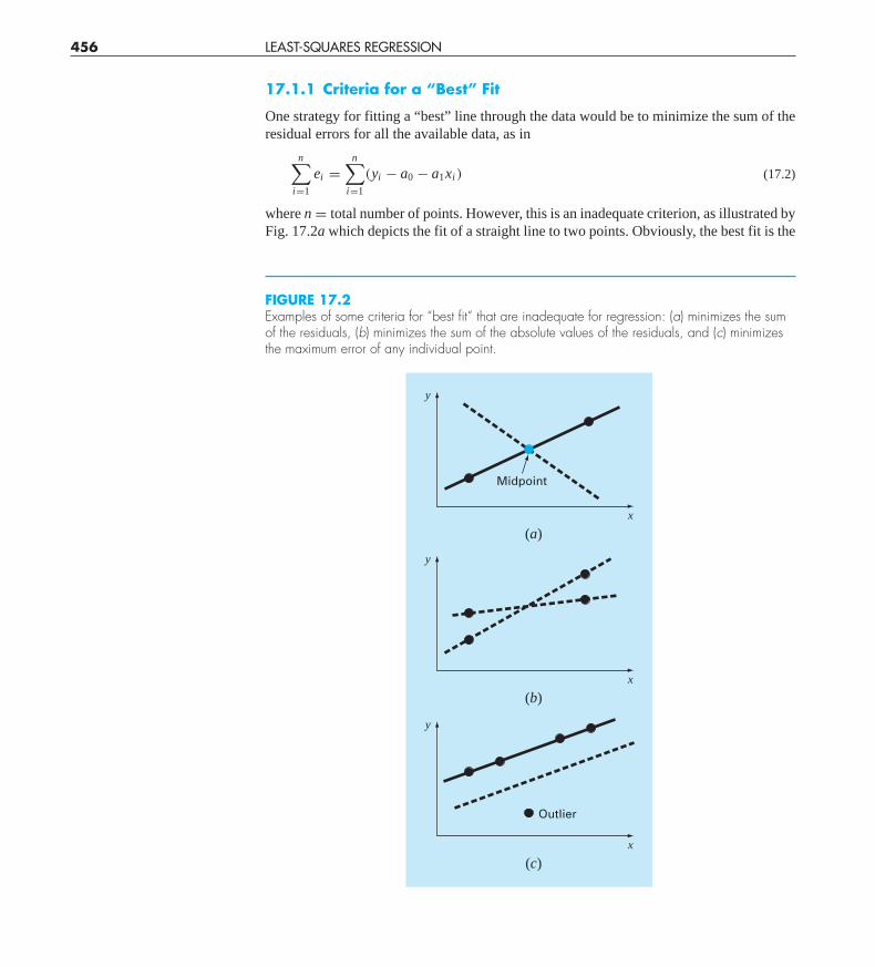
where n = total number of points. However, this is an inadequate criterion, as illustrated byFig. 17.2a which depicts the fit of a straight line to two points. Obviously, the best fit is the

456 LEAST-SQUARES REGRESSION

y

Midpoint

Outlier

x

(a)

y

x

(b)

y

x

(c)

FIGURE 17.2Examples of some criteria for “best fit” that are inadequate for regression: (a) minimizes the sumof the residuals, (b) minimizes the sum of the absolute values of the residuals, and (c) minimizesthe maximum error of any individual point.

cha01064_ch17.qxd 3/20/09 12:43 PM Page 456

line connecting the points. However, any straight line passing through the midpoint of theconnecting line (except a perfectly vertical line) results in a minimum value of Eq. (17.2)equal to zero because the errors cancel.

Therefore, another logical criterion might be to minimize the sum of the absolute val-ues of the discrepancies, as in

n∑i=1

|ei | =n∑

i=1

|yi − a0 − a1xi |

Figure 17.2b demonstrates why this criterion is also inadequate. For the four points shown,any straight line falling within the dashed lines will minimize the sum of the absolutevalues. Thus, this criterion also does not yield a unique best fit.

A third strategy for fitting a best line is the minimax criterion. In this technique, the lineis chosen that minimizes the maximum distance that an individual point falls from theline. As depicted in Fig. 17.2c, this strategy is ill-suited for regression because it givesundue influence to an outlier, that is, a single point with a large error. It should be noted thatthe minimax principle is sometimes well-suited for fitting a simple function to a compli-cated function (Carnahan, Luther, and Wilkes, 1969).

A strategy that overcomes the shortcomings of the aforementioned approaches is tominimize the sum of the squares of the residuals between the measured y and the y calcu-lated with the linear model

Sr =n∑

i=1

e2i =

n∑i=1

(yi,measured − yi,model)2 =

n∑i=1

(yi − a0 − a1xi )2 (17.3)

This criterion has a number of advantages, including the fact that it yields a unique line fora given set of data. Before discussing these properties, we will present a technique for de-termining the values of a0 and a1 that minimize Eq. (17.3).

17.1.2 Least-Squares Fit of a Straight Line

To determine values for a0 and a1, Eq. (17.3) is differentiated with respect to each coeffi-cient:

∂Sr

∂a0= −2

∑(yi − a0 − a1xi )

∂Sr

∂a1= −2

∑[(yi − a0 − a1xi )xi ]

Note that we have simplified the summation symbols; unless otherwise indicated, all sum-mations are from i = 1 to n. Setting these derivatives equal to zero will result in a minimumSr. If this is done, the equations can be expressed as

0 =∑

yi −∑

a0 −∑

a1xi

0 =∑

yi xi −∑

a0xi −∑

a1x2i


cha01064_ch17.qxd 3/20/09 12:43 PM 57

Now, realizing that �a0 = na0, we can express the equations as a set of two simultaneouslinear equations with two unknowns (a0 and a1):

na0 +(∑

xi

)a1 =

∑yi (17.4)(∑

xi

)a0 +

(∑x2

i

)a1 =

∑xi yi (17.5)

These are called the normal equations. They can be solved simultaneously

a1 = n�xi yi − �xi�yi

n�x2i − (�xi )2

(17.6)

This result can then be used in conjunction with Eq. (17.4) to solve for

a0 = y − a1 x (17.7)

where y and x are the means of y and x, respectively.

EXAMPLE 17.1 Linear Regression

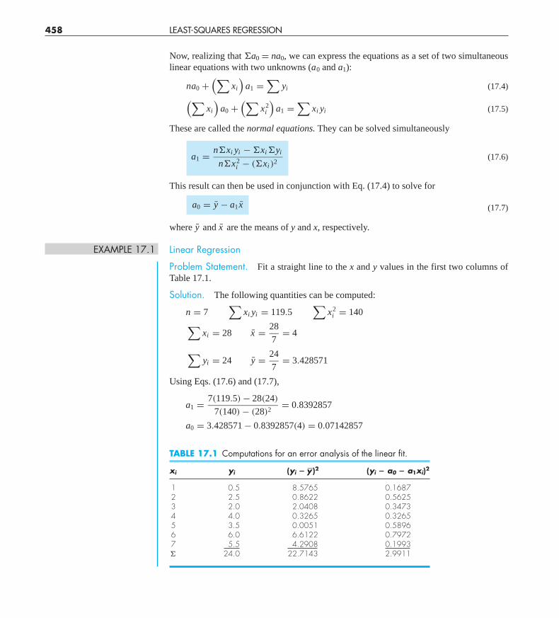
Problem Statement. Fit a straight line to the x and y values in the first two columns ofTable 17.1.

Solution. The following quantities can be computed:

n = 7∑

xi yi = 119.5∑

x2i = 140∑

xi = 28 x = 28

7= 4

∑yi = 24 y = 24

7= 3.428571

Using Eqs. (17.6) and (17.7),

a1 = 7(119.5) − 28(24)

7(140) − (28)2= 0.8392857

a0 = 3.428571 − 0.8392857(4) = 0.07142857


TABLE 17.1 Computations for an error analysis of the linear fit.

xi yi (yi � y�)2 (yi � a0 � a1xi)2

1 0.5 8.5765 0.16872 2.5 0.8622 0.56253 2.0 2.0408 0.34734 4.0 0.3265 0.32655 3.5 0.0051 0.58966 6.0 6.6122 0.79727 5.5 4.2908 0.1993� 24.0 22.7143 2.9911

cha01064_ch17.qxd 3/20/09 12:43 PM Page 458

Therefore, the least-squares fit is

y = 0.07142857 + 0.8392857x

The line, along with the data, is shown in Fig. 17.1c.

17.1.3 Quantification of Error of Linear Regression

Any line other than the one computed in Example 17.1 results in a larger sum of the squaresof the residuals. Thus, the line is unique and in terms of our chosen criterion is a “best” linethrough the points. A number of additional properties of this fit can be elucidated by ex-amining more closely the way in which residuals were computed. Recall that the sum of thesquares is defined as [Eq. (17.3)]

Sr =n∑

i=1

e2i =

n∑i=1

(yi − a0 − a1xi )2 (17.8)

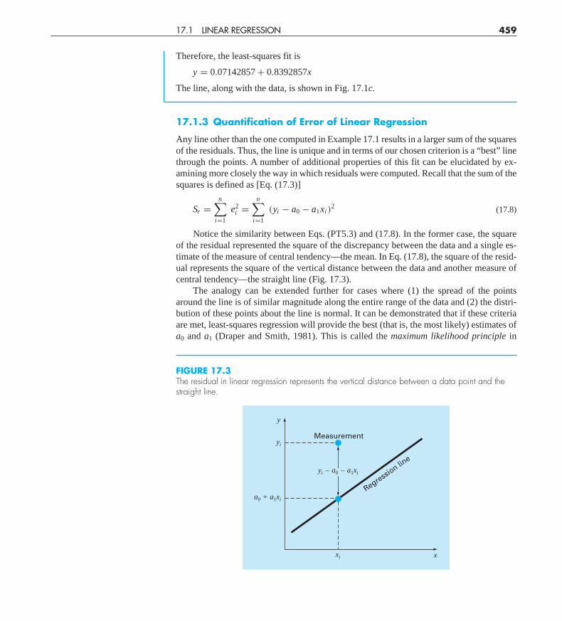
Notice the similarity between Eqs. (PT5.3) and (17.8). In the former case, the squareof the residual represented the square of the discrepancy between the data and a single es-timate of the measure of central tendency—the mean. In Eq. (17.8), the square of the resid-ual represents the square of the vertical distance between the data and another measure ofcentral tendency—the straight line (Fig. 17.3).

The analogy can be extended further for cases where (1) the spread of the pointsaround the line is of similar magnitude along the entire range of the data and (2) the distri-bution of these points about the line is normal. It can be demonstrated that if these criteriaare met, least-squares regression will provide the best (that is, the most likely) estimates ofa0 and a1 (Draper and Smith, 1981). This is called the maximum likelihood principle in


FIGURE 17.3The residual in linear regression represents the vertical distance between a data point and thestraight line.

y

yi

xi

a0 + a1xi

Measurement

yi – a0 – a1xi

Regression lin

e

x

cha01064_ch17.qxd 3/20/09 12:43 PM Page 459

statistics. In addition, if these criteria are met, a “standard deviation” for the regression linecan be determined as [compare with Eq. (PT5.2)]

sy/x =√

Sr

n − 2(17.9)

where sy/x is called the standard error of the estimate. The subscript notation “y/x” desig-nates that the error is for a predicted value of y corresponding to a particular value of x.Also, notice that we now divide by n − 2 because two data-derived estimates—a0 and a1—were used to compute Sr; thus, we have lost two degrees of freedom. As with our discus-sion of the standard deviation in PT5.2.1, another justification for dividing by n − 2 is thatthere is no such thing as the “spread of data” around a straight line connecting two points.Thus, for the case where n = 2, Eq. (17.9) yields a meaningless result of infinity.

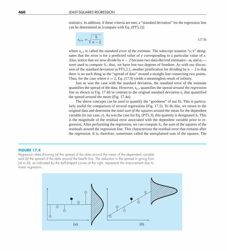
Just as was the case with the standard deviation, the standard error of the estimatequantifies the spread of the data. However, sy/x quantifies the spread around the regressionline as shown in Fig. 17.4b in contrast to the original standard deviation sy that quantifiedthe spread around the mean (Fig. 17.4a).

The above concepts can be used to quantify the “goodness” of our fit. This is particu-larly useful for comparison of several regressions (Fig. 17.5). To do this, we return to theoriginal data and determine the total sum of the squares around the mean for the dependentvariable (in our case, y). As was the case for Eq. (PT5.3), this quantity is designated St. Thisis the magnitude of the residual error associated with the dependent variable prior to re-gression. After performing the regression, we can compute Sr, the sum of the squares of theresiduals around the regression line. This characterizes the residual error that remains afterthe regression. It is, therefore, sometimes called the unexplained sum of the squares. The


FIGURE 17.4Regression data showing (a) the spread of the data around the mean of the dependent variableand (b) the spread of the data around the best-fit line. The reduction in the spread in going from(a) to (b), as indicated by the bell-shaped curves at the right, represents the improvement due tolinear regression.

(a) (b)

cha01064_ch17.qxd 3/20/09 12:43 PM Page 460

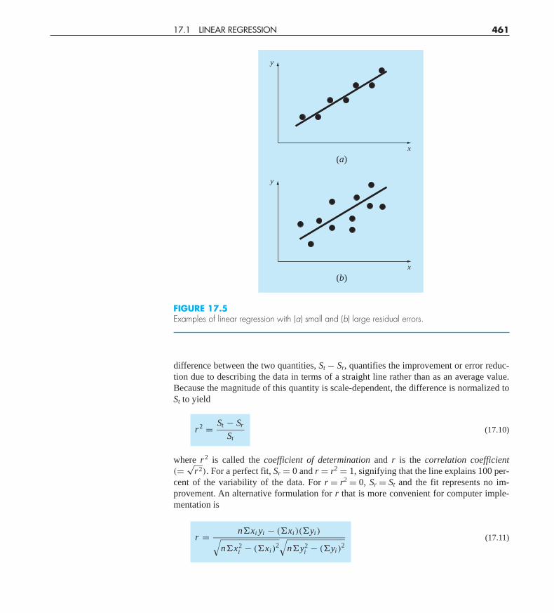
difference between the two quantities, St − Sr, quantifies the improvement or error reduc-tion due to describing the data in terms of a straight line rather than as an average value.Because the magnitude of this quantity is scale-dependent, the difference is normalized toSt to yield

r2 = St − Sr

St(17.10)

where r2 is called the coefficient of determination and r is the correlation coefficient(=

√r2). For a perfect fit, Sr = 0 and r = r2 = 1, signifying that the line explains 100 per-

cent of the variability of the data. For r = r2 = 0, Sr = St and the fit represents no im-provement. An alternative formulation for r that is more convenient for computer imple-mentation is

r = n�xi yi − (�xi )(�yi )√n�x2

i − (�xi )2√

n�y2i − (�yi )

2(17.11)


FIGURE 17.5Examples of linear regression with (a) small and (b) large residual errors.

y

x

(a)

y

x

(b)

cha01064_ch17.qxd 3/20/09 12:43 PM Page 461

EXAMPLE 17.2 Estimation of Errors for the Linear Least-Squares Fit

Problem Statement. Compute the total standard deviation, the standard error of the esti-mate, and the correlation coefficient for the data in Example 17.1.

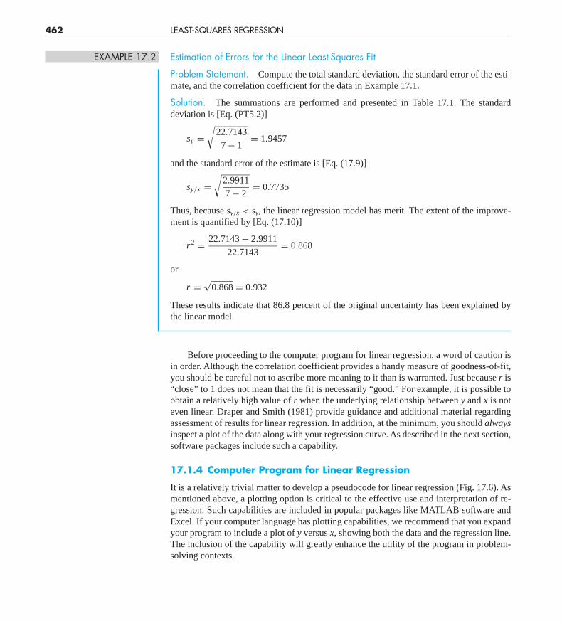
Solution. The summations are performed and presented in Table 17.1. The standarddeviation is [Eq. (PT5.2)]

sy =√

22.7143

7 − 1= 1.9457

and the standard error of the estimate is [Eq. (17.9)]

sy/x =√

2.9911

7 − 2= 0.7735

Thus, because sy/x < sy, the linear regression model has merit. The extent of the improve-ment is quantified by [Eq. (17.10)]

r2 = 22.7143 − 2.9911

22.7143= 0.868

or

r =√

0.868 = 0.932

These results indicate that 86.8 percent of the original uncertainty has been explained bythe linear model.

Before proceeding to the computer program for linear regression, a word of caution isin order. Although the correlation coefficient provides a handy measure of goodness-of-fit,you should be careful not to ascribe more meaning to it than is warranted. Just because r is“close” to 1 does not mean that the fit is necessarily “good.” For example, it is possible toobtain a relatively high value of r when the underlying relationship between y and x is noteven linear. Draper and Smith (1981) provide guidance and additional material regardingassessment of results for linear regression. In addition, at the minimum, you should alwaysinspect a plot of the data along with your regression curve. As described in the next section,software packages include such a capability.

17.1.4 Computer Program for Linear Regression

It is a relatively trivial matter to develop a pseudocode for linear regression (Fig. 17.6). Asmentioned above, a plotting option is critical to the effective use and interpretation of re-gression. Such capabilities are included in popular packages like MATLAB software andExcel. If your computer language has plotting capabilities, we recommend that you expandyour program to include a plot of y versus x, showing both the data and the regression line.The inclusion of the capability will greatly enhance the utility of the program in problem-solving contexts.


cha01064_ch17.qxd 3/20/09 12:43 PM Page 462

EXAMPLE 17.3 Linear Regression Using the Computer

Problem Statement. We can use software based on Fig. 17.6 to solve a hypothesis-testing problem associated with the falling parachutist discussed in Chap. 1. A theoreticalmathematical model for the velocity of the parachutist was given as the following[Eq. (1.10)]:

v(t) = gm

c

(1 − e(−c/m)t

)where v = velocity (m/s), g = gravitational constant (9.8 m/s2), m = mass of the para-chutist equal to 68.1 kg, and c = drag coefficient of 12.5 kg/s. The model predicts the ve-locity of the parachutist as a function of time, as described in Example 1.1.

An alternative empirical model for the velocity of the parachutist is given by

v(t) = gm

c

(t

3.75 + t

)(E17.3.1)

Suppose that you would like to test and compare the adequacy of these two mathemat-ical models. This might be accomplished by measuring the actual velocity of the parachutist


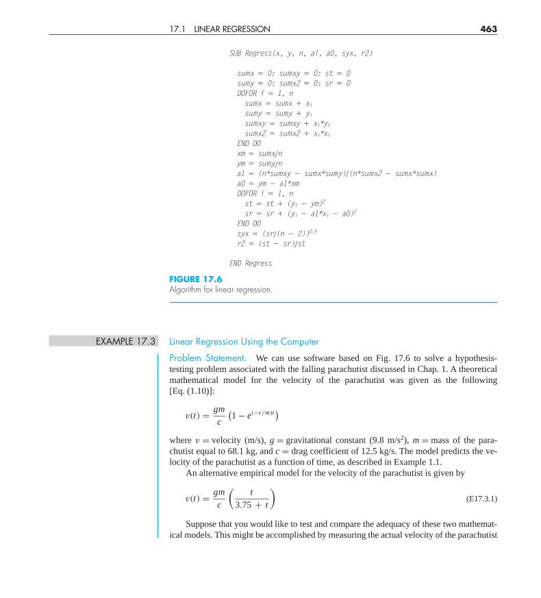
SUB Regress(x, y, n, al, a0, syx, r2)

sumx � 0: sumxy � 0: st � 0sumy � 0: sumx2 � 0: sr � 0DOFOR i � 1, nsumx � sumx � xisumy � sumy � yisumxy � sumxy � xi*yisumx2 � sumx2 � xi*xi

END DOxm � sumx/nym � sumy/na1 � (n*sumxy � sumx*sumy)�(n*sumx2 � sumx*sumx)a0 � ym � a1*xmDOFOR i � 1, nst � st � (yi � ym)2

sr � sr � (yi � a1*xi � a0)2

END DOsyx � (sr/(n � 2))0.5

r2 � (st � sr)/st

END Regress

FIGURE 17.6Algorithm for linear regression.

cha01064_ch17.qxd 3/20/09 12:43 PM Page 463

at known values of time and comparing these results with the predicted velocities accordingto each model.

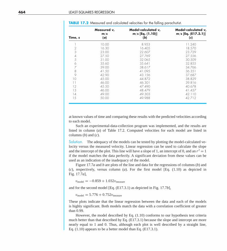
Such an experimental-data-collection program was implemented, and the results arelisted in column (a) of Table 17.2. Computed velocities for each model are listed incolumns (b) and (c).

Solution. The adequacy of the models can be tested by plotting the model-calculated ve-locity versus the measured velocity. Linear regression can be used to calculate the slopeand the intercept of the plot. This line will have a slope of 1, an intercept of 0, and an r2 = 1if the model matches the data perfectly. A significant deviation from these values can beused as an indication of the inadequacy of the model.

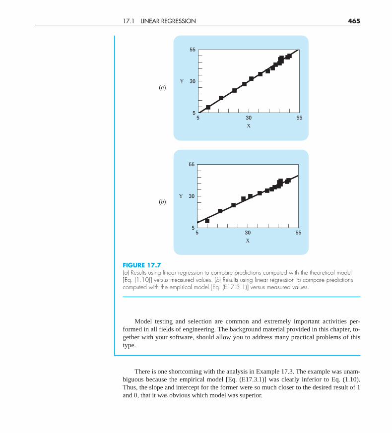
Figure 17.7a and b are plots of the line and data for the regressions of columns (b) and(c), respectively, versus column (a). For the first model [Eq. (1.10) as depicted inFig. 17.7a],

vmodel = −0.859 + 1.032vmeasure

and for the second model [Eq. (E17.3.1) as depicted in Fig. 17.7b],

vmodel = 5.776 + 0.752vmeasure

These plots indicate that the linear regression between the data and each of the modelsis highly significant. Both models match the data with a correlation coefficient of greaterthan 0.99.

However, the model described by Eq. (1.10) conforms to our hypothesis test criteriamuch better than that described by Eq. (E17.3.1) because the slope and intercept are morenearly equal to 1 and 0. Thus, although each plot is well described by a straight line,Eq. (1.10) appears to be a better model than Eq. (E17.3.1).


TABLE 17.2 Measured and calculated velocities for the falling parachutist.

Measured v, Model-calculated v, Model-calculated v,m/s m/s [Eq. (1.10)] m/s [Eq. (E17.3.1)]

Time, s (a) (b) (c)

1 10.00 8.953 11.2402 16.30 16.405 18.5703 23.00 22.607 23.7294 27.50 27.769 27.5565 31.00 32.065 30.5096 35.60 35.641 32.8557 39.00 38.617 34.7668 41.50 41.095 36.3519 42.90 43.156 37.687

10 45.00 44.872 38.82911 46.00 46.301 39.81612 45.50 47.490 40.67813 46.00 48.479 41.43714 49.00 49.303 42.11015 50.00 49.988 42.712

cha01064_ch17.qxd 3/20/09 12:43 PM Page 464

Model testing and selection are common and extremely important activities per-formed in all fields of engineering. The background material provided in this chapter, to-gether with your software, should allow you to address many practical problems of thistype.

There is one shortcoming with the analysis in Example 17.3. The example was unam-biguous because the empirical model [Eq. (E17.3.1)] was clearly inferior to Eq. (1.10).Thus, the slope and intercept for the former were so much closer to the desired result of 1and 0, that it was obvious which model was superior.


FIGURE 17.7(a) Results using linear regression to compare predictions computed with the theoretical model[Eq. (1.10)] versus measured values. (b) Results using linear regression to compare predictionscomputed with the empirical model [Eq. (E17.3.1)] versus measured values.

55

30Y

5 30

X

555

(a)

55

30Y

5 30

X

555

(b)

(a)

(b)

cha01064_ch17.qxd 3/20/09 12:43 PM Page 465

However, suppose that the slope were 0.85 and the intercept were 2. Obviously thiswould make the conclusion that the slope and intercept were 1 and 0 open to debate.Clearly, rather than relying on a subjective judgment, it would be preferable to base such aconclusion on a quantitative criterion.

This can be done by computing confidence intervals for the model parameters in thesame way that we developed confidence intervals for the mean in Sec. PT5.2.3. We will re-turn to this topic at the end of this chapter.

17.1.5 Linearization of Nonlinear Relationships

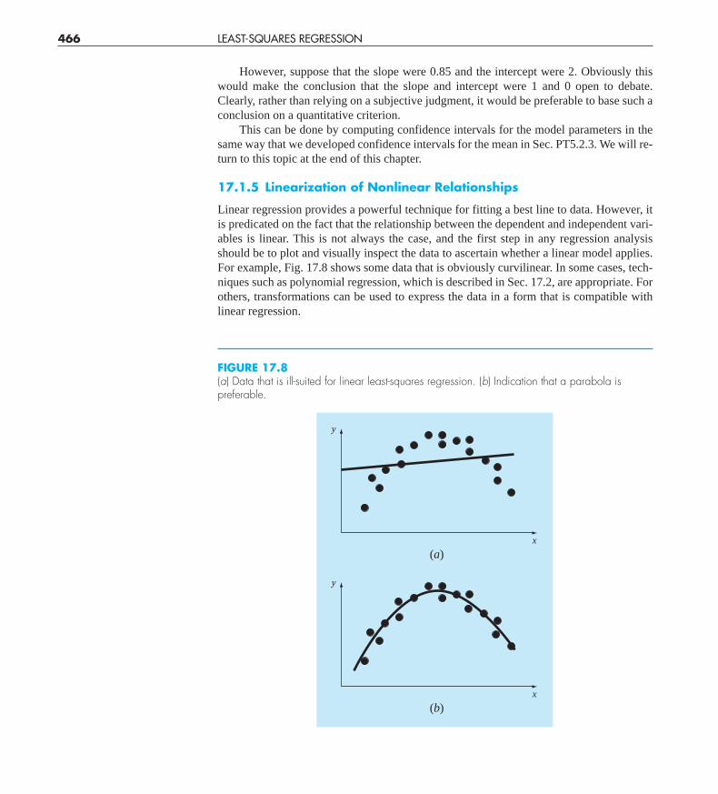
Linear regression provides a powerful technique for fitting a best line to data. However, itis predicated on the fact that the relationship between the dependent and independent vari-ables is linear. This is not always the case, and the first step in any regression analysisshould be to plot and visually inspect the data to ascertain whether a linear model applies.For example, Fig. 17.8 shows some data that is obviously curvilinear. In some cases, tech-niques such as polynomial regression, which is described in Sec. 17.2, are appropriate. Forothers, transformations can be used to express the data in a form that is compatible withlinear regression.


FIGURE 17.8(a) Data that is ill-suited for linear least-squares regression. (b) Indication that a parabola ispreferable.

y

x

(a)

y

x

(b)

cha01064_ch17.qxd 3/20/09 12:44 PM Page 466

One example is the exponential model

y = α1eβ1x (17.12)

where α1 and β1 are constants. This model is used in many fields of engineering to charac-terize quantities that increase (positive β1) or decrease (negative β1) at a rate that is directlyproportional to their own magnitude. For example, population growth or radioactive decaycan exhibit such behavior. As depicted in Fig. 17.9a, the equation represents a nonlinear re-lationship (for β1 �= 0) between y and x.

Another example of a nonlinear model is the simple power equation

y = α2xβ2 (17.13)


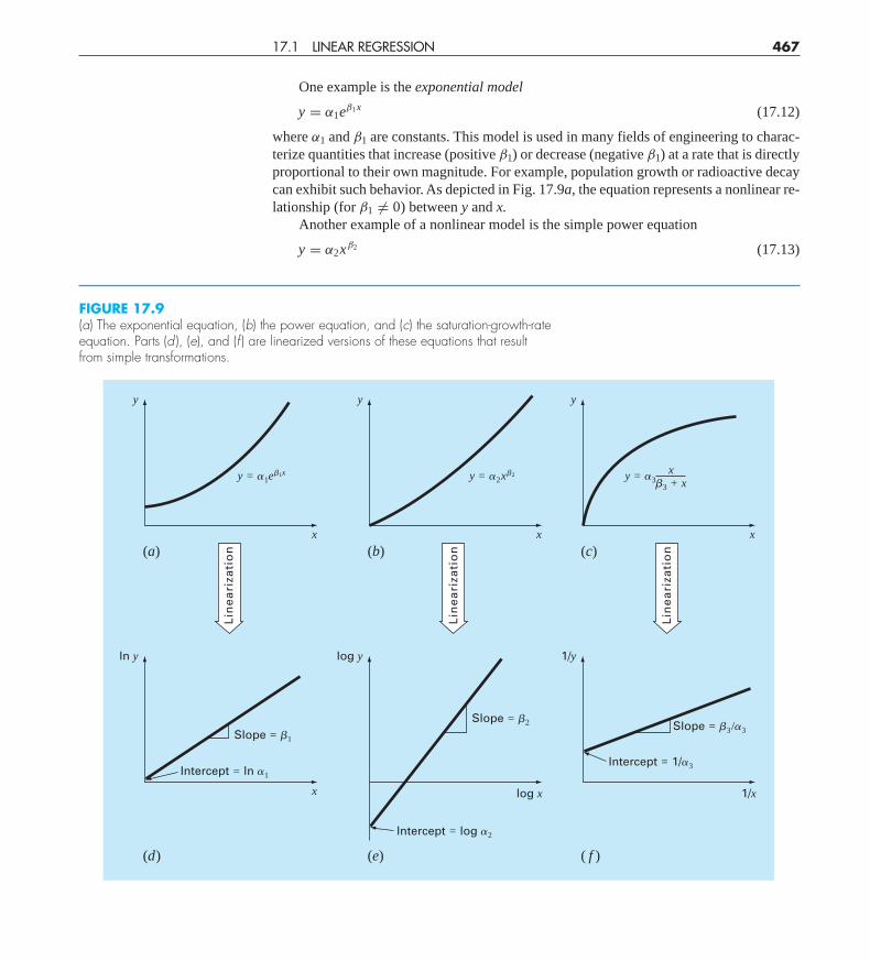
FIGURE 17.9(a) The exponential equation, (b) the power equation, and (c) the saturation-growth-rateequation. Parts (d ), (e), and (f ) are linearized versions of these equations that resultfrom simple transformations.

y

x

y = �1e�1x

(a)

Lin

ea

riza

tio

n

y

x

y = �2x�2

(b)

Lin

ea

riza

tio

n

y

x

(c)

Lin

ea

riza

tio

n

y = �3x

�3 + x

ln y

x

Slope = �1

Intercept = ln �1

(d)

log y

log x

(e)

1/y

1/x

( f )

Intercept = log �2

Intercept = 1/�3

Slope = �2 Slope = �3/�3

cha01064_ch17.qxd 3/20/09 12:44 PM Page 467

where α2 and β2 are constant coefficients. This model has wide applicability in all fields ofengineering. As depicted in Fig. 17.9b, the equation (for β2 �= 0 or 1) is nonlinear.

A third example of a nonlinear model is the saturation-growth-rate equation [recallEq. (E17.3.1)]

y = α3x

β3 + x(17.14)

where α3 and β3 are constant coefficients. This model, which is particularly well-suited forcharacterizing population growth rate under limiting conditions, also represents a nonlin-ear relationship between y and x (Fig. 17.9c) that levels off, or “saturates,” as x increases.

Nonlinear regression techniques are available to fit these equations to experimentaldata directly. (Note that we will discuss nonlinear regression in Sec. 17.5.) However, a sim-pler alternative is to use mathematical manipulations to transform the equations into a lin-ear form. Then, simple linear regression can be employed to fit the equations to data.

For example, Eq. (17.12) can be linearized by taking its natural logarithm to yield

ln y = ln α1 + β1x ln e

But because ln e = 1,

ln y = ln α1 + β1x (17.15)

Thus, a plot of ln y versus x will yield a straight line with a slope of β1 and an intercept ofln α1 (Fig. 17.9d ).

Equation (17.13) is linearized by taking its base-10 logarithm to give

log y = β2 log x + log α2 (17.16)

Thus, a plot of log y versus log x will yield a straight line with a slope of β2 and an inter-cept of log α2 (Fig. 17.9e).

Equation (17.14) is linearized by inverting it to give

1

y= β3

α3

1

x+ 1

α3(17.17)

Thus, a plot of 1/y versus l/x will be linear, with a slope of β3/α3 and an intercept of 1/α3

(Fig. 17.9f ).In their transformed forms, these models can use linear regression to evaluate the con-

stant coefficients. They could then be transformed back to their original state and used forpredictive purposes. Example 17.4 illustrates this procedure for Eq. (17.13). In addition,Sec. 20.1 provides an engineering example of the same sort of computation.

EXAMPLE 17.4 Linearization of a Power Equation

Problem Statement. Fit Eq. (17.13) to the data in Table 17.3 using a logarithmic trans-formation of the data.

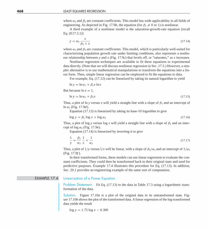
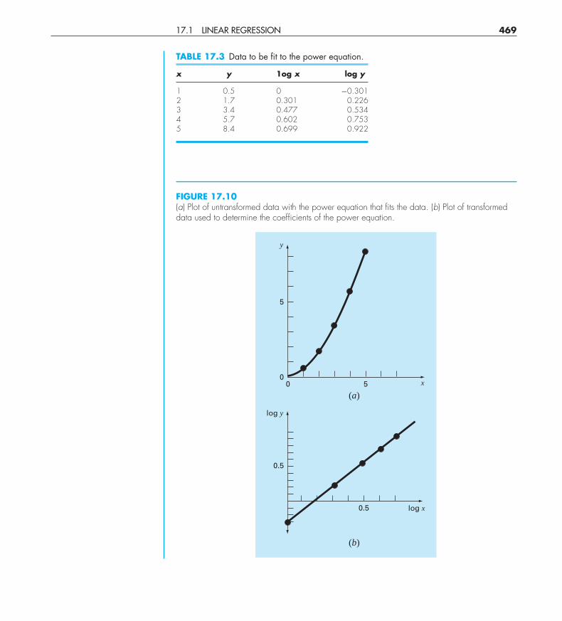
Solution. Figure 17.10a is a plot of the original data in its untransformed state. Fig-ure 17.10b shows the plot of the transformed data. A linear regression of the log-transformeddata yields the result

log y = 1.75 log x − 0.300


cha01064_ch17.qxd 3/20/09 12:44 PM Page 468


FIGURE 17.10(a) Plot of untransformed data with the power equation that fits the data. (b) Plot of transformeddata used to determine the coefficients of the power equation.

y

x500

5

(a)

log y

0.5

(b)

log x0.5

TABLE 17.3 Data to be fit to the power equation.

x y 1og x log y

1 0.5 0 −0.3012 1.7 0.301 0.2263 3.4 0.477 0.5344 5.7 0.602 0.7535 8.4 0.699 0.922

cha01064_ch17.qxd 3/20/09 12:44 PM Page 469

Thus, the intercept, log α2, equals −0.300, and therefore, by taking the antilogarithm, α2 =10−0.3 = 0.5. The slope is β2 = 1.75. Consequently, the power equation is

y = 0.5x1.75

This curve, as plotted in Fig. 17.10a, indicates a good fit.

17.1.6 General Comments on Linear Regression

Before proceeding to curvilinear and multiple linear regression, we must emphasize theintroductory nature of the foregoing material on linear regression. We have focused on thesimple derivation and practical use of equations to fit data. You should be cognizant ofthe fact that there are theoretical aspects of regression that are of practical importance butare beyond the scope of this book. For example, some statistical assumptions that are in-herent in the linear least-squares procedures are

1. Each x has a fixed value; it is not random and is known without error.2. The y values are independent random variables and all have the same variance.3. The y values for a given x must be normally distributed.

Such assumptions are relevant to the proper derivation and use of regression. For ex-ample, the first assumption means that (1) the x values must be error-free and (2) the re-gression of y versus x is not the same as x versus y (try Prob. 17.4 at the end of the chapter).You are urged to consult other references such as Draper and Smith (1981) to appreciateaspects and nuances of regression that are beyond the scope of this book.

17.2 POLYNOMIAL REGRESSION

In Sec. 17.1, a procedure was developed to derive the equation of a straight line using theleast-squares criterion. Some engineering data, although exhibiting a marked pattern suchas seen in Fig. 17.8, is poorly represented by a straight line. For these cases, a curve wouldbe better suited to fit the data. As discussed in the previous section, one method to accom-plish this objective is to use transformations. Another alternative is to fit polynomials to thedata using polynomial regression.

The least-squares procedure can be readily extended to fit the data to a higher-orderpolynomial. For example, suppose that we fit a second-order polynomial or quadratic:

y = a0 + a1x + a2x2 + e

For this case the sum of the squares of the residuals is [compare with Eq. (17.3)]

Sr =n∑

i=1

(yi − a0 − a1xi − a2x2

i

)2(17.18)

Following the procedure of the previous section, we take the derivative of Eq. (17.18) withrespect to each of the unknown coefficients of the polynomial, as in

∂Sr

∂a0= −2

∑(yi − a0 − a1xi − a2x2

i

)


cha01064_ch17.qxd 3/20/09 12:44 PM Page 470

∂Sr

∂a1= −2

∑xi

(yi − a0 − a1xi − a2x2

i

)∂Sr

∂a2= −2

∑x2

i

(yi − a0 − a1xi − a2x2

i

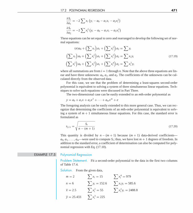
)These equations can be set equal to zero and rearranged to develop the following set of nor-mal equations:

(n)a0 +(∑

xi

)a1 +

(∑x2

i

)a2 =

∑yi(∑

xi

)a0 +

(∑x2

i

)a1 +

(∑x3

i

)a2 =

∑xi yi(∑

x2i

)a0 +

(∑x3

i

)a1 +

(∑x4

i

)a2 =

∑x2

i yi

(17.19)

where all summations are from i = 1 through n. Note that the above three equations are lin-ear and have three unknowns: a0, a1, and a2. The coefficients of the unknowns can be cal-culated directly from the observed data.

For this case, we see that the problem of determining a least-squares second-orderpolynomial is equivalent to solving a system of three simultaneous linear equations. Tech-niques to solve such equations were discussed in Part Three.

The two-dimensional case can be easily extended to an mth-order polynomial as

y = a0 + a1x + a2x2 + · · · + am xm + e

The foregoing analysis can be easily extended to this more general case. Thus, we can rec-ognize that determining the coefficients of an mth-order polynomial is equivalent to solv-ing a system of m + 1 simultaneous linear equations. For this case, the standard error isformulated as

sy/x =√

Sr

n − (m + 1)(17.20)

This quantity is divided by n − (m + 1) because (m + 1) data-derived coefficients—a0, a1, . . . , am—were used to compute Sr; thus, we have lost m + 1 degrees of freedom. Inaddition to the standard error, a coefficient of determination can also be computed for poly-nomial regression with Eq. (17.10).

EXAMPLE 17.5 Polynomial Regression

Problem Statement. Fit a second-order polynomial to the data in the first two columnsof Table 17.4.

Solution. From the given data,

m = 2∑

xi = 15∑

x4i = 979

n = 6∑

yi = 152.6∑

xi yi = 585.6

x = 2.5∑

x2i = 55

∑x2

i yi = 2488.8

y = 25.433∑

x3i = 225

17.2 POLYNOMIAL REGRESSION 471

cha01064_ch17.qxd 3/20/09 12:44 PM Page 471

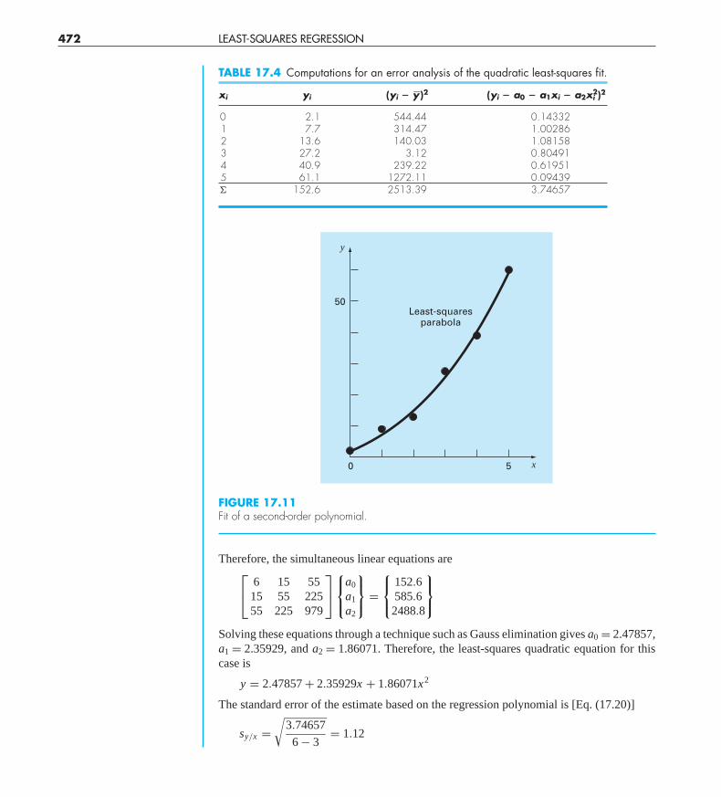
Therefore, the simultaneous linear equations are⎡⎣ 6 15 55

15 55 22555 225 979

⎤⎦

⎧⎨⎩

a0

a1

a2

⎫⎬⎭ =

⎧⎨⎩

152.6585.62488.8

⎫⎬⎭

Solving these equations through a technique such as Gauss elimination gives a0 = 2.47857,a1 = 2.35929, and a2 = 1.86071. Therefore, the least-squares quadratic equation for thiscase is

y = 2.47857 + 2.35929x + 1.86071x2

The standard error of the estimate based on the regression polynomial is [Eq. (17.20)]

sy/x =√

3.74657

6 − 3= 1.12


FIGURE 17.11Fit of a second-order polynomial.

y

x50

50Least-squares

parabola

TABLE 17.4 Computations for an error analysis of the quadratic least-squares fit.

xi yi (yi � y�)2 (yi � a0 � a1xi � a2xi2)2

0 2.1 544.44 0.143321 7.7 314.47 1.002862 13.6 140.03 1.081583 27.2 3.12 0.804914 40.9 239.22 0.619515 61.1 1272.11 0.09439� 152.6 2513.39 3.74657

cha01064_ch17.qxd 3/20/09 12:44 PM Page 472

The coefficient of determination is

r2 = 2513.39 − 3.74657

2513.39= 0.99851

and the correlation coefficient is r = 0.99925.These results indicate that 99.851 percent of the original uncertainty has been ex-

plained by the model. This result supports the conclusion that the quadratic equation rep-resents an excellent fit, as is also evident from Fig. 17.11.

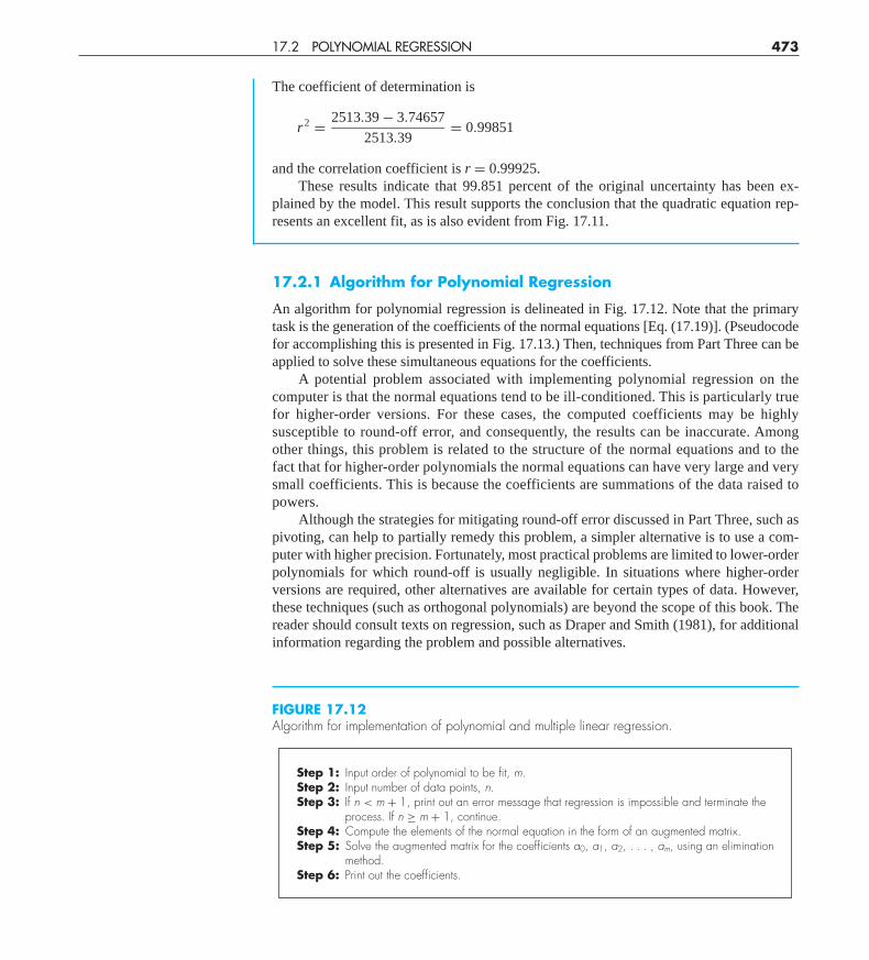
17.2.1 Algorithm for Polynomial Regression

An algorithm for polynomial regression is delineated in Fig. 17.12. Note that the primarytask is the generation of the coefficients of the normal equations [Eq. (17.19)]. (Pseudocodefor accomplishing this is presented in Fig. 17.13.) Then, techniques from Part Three can beapplied to solve these simultaneous equations for the coefficients.

A potential problem associated with implementing polynomial regression on thecomputer is that the normal equations tend to be ill-conditioned. This is particularly truefor higher-order versions. For these cases, the computed coefficients may be highlysusceptible to round-off error, and consequently, the results can be inaccurate. Amongother things, this problem is related to the structure of the normal equations and to thefact that for higher-order polynomials the normal equations can have very large and verysmall coefficients. This is because the coefficients are summations of the data raised topowers.

Although the strategies for mitigating round-off error discussed in Part Three, such aspivoting, can help to partially remedy this problem, a simpler alternative is to use a com-puter with higher precision. Fortunately, most practical problems are limited to lower-orderpolynomials for which round-off is usually negligible. In situations where higher-orderversions are required, other alternatives are available for certain types of data. However,these techniques (such as orthogonal polynomials) are beyond the scope of this book. Thereader should consult texts on regression, such as Draper and Smith (1981), for additionalinformation regarding the problem and possible alternatives.

17.2 POLYNOMIAL REGRESSION 473

FIGURE 17.12Algorithm for implementation of polynomial and multiple linear regression.

Step 1: Input order of polynomial to be fit, m.Step 2: Input number of data points, n.Step 3: If n < m + 1, print out an error message that regression is impossible and terminate the

process. If n ≥ m + 1, continue.Step 4: Compute the elements of the normal equation in the form of an augmented matrix.Step 5: Solve the augmented matrix for the coefficients a0, a1, a2, . . . , am, using an elimination

method.Step 6: Print out the coefficients.

cha01064_ch17.qxd 3/20/09 12:44 PM Page 473

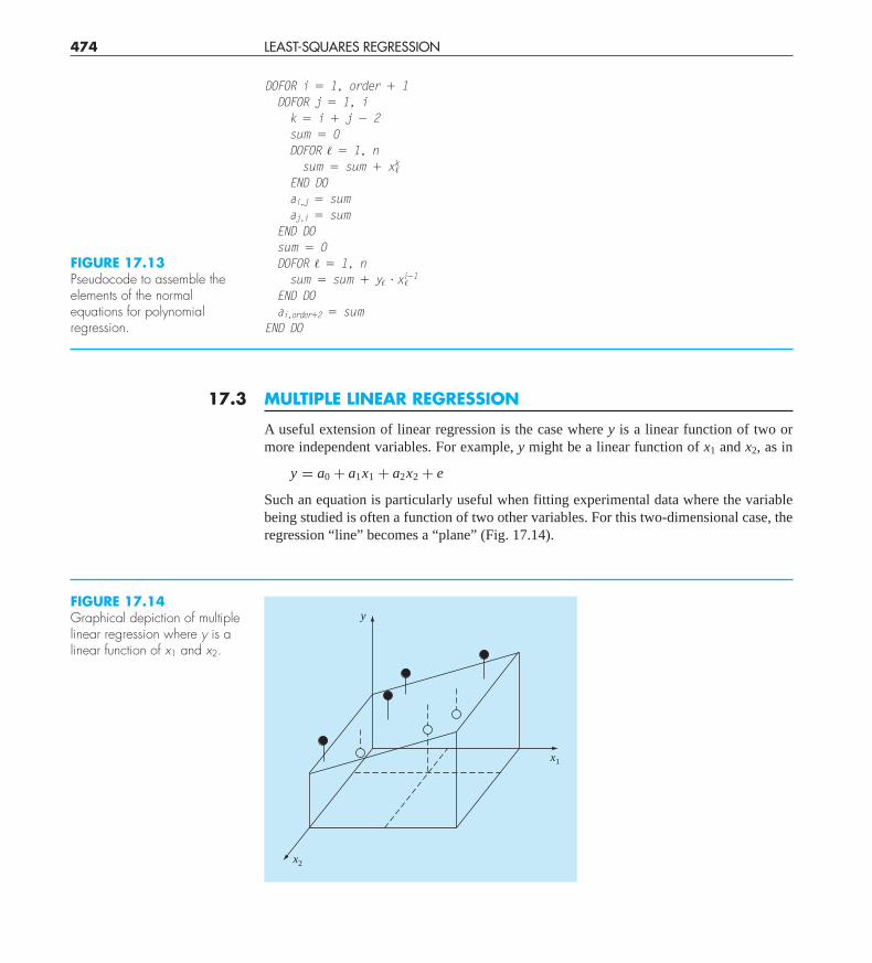
17.3 MULTIPLE LINEAR REGRESSION

A useful extension of linear regression is the case where y is a linear function of two ormore independent variables. For example, y might be a linear function of x1 and x2, as in

y = a0 + a1x1 + a2x2 + e

Such an equation is particularly useful when fitting experimental data where the variablebeing studied is often a function of two other variables. For this two-dimensional case, theregression “line” becomes a “plane” (Fig. 17.14).


DOFOR i � 1, order � 1DOFOR j � 1, ik � i � j � 2sum � 0DOFOR � � 1, nsum � sum � xk�

END DOai,j � sumaj,i � sum

END DOsum � 0DOFOR � � 1, nsum � sum � y� � xi�1�

END DOai,order�2 � sum

END DO

FIGURE 17.13Pseudocode to assemble theelements of the normalequations for polynomialregression.

FIGURE 17.14Graphical depiction of multiplelinear regression where y is alinear function of x1 and x2.

y

x1

x2

cha01064_ch17.qxd 3/20/09 12:44 PM Page 474

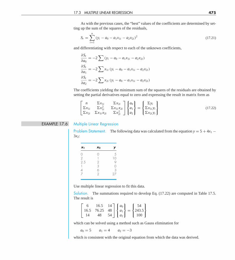
As with the previous cases, the “best” values of the coefficients are determined by set-ting up the sum of the squares of the residuals,

Sr =n∑

i=1

(yi − a0 − a1x1i − a2x2i )2 (17.21)

and differentiating with respect to each of the unknown coefficients,

∂Sr

∂a0= −2

∑(yi − a0 − a1x1i − a2x2i )

∂Sr

∂a1= −2

∑x1i (yi − a0 − a1x1i − a2x2i )

∂Sr

∂a2= −2

∑x2i (yi − a0 − a1x1i − a2x2i )

The coefficients yielding the minimum sum of the squares of the residuals are obtained bysetting the partial derivatives equal to zero and expressing the result in matrix form as⎡

⎣ n �x1i �x2i

�x1i �x21i �x1i x2i

�x2i �x1i x2i �x22i

⎤⎦

⎧⎨⎩

a0

a1

a2

⎫⎬⎭ =

⎧⎨⎩

�yi

�x1i yi

�x2i yi

⎫⎬⎭ (17.22)

EXAMPLE 17.6 Multiple Linear Regression

Problem Statement. The following data was calculated from the equation y = 5 + 4x1 −3x2:

x1 x2 y

0 0 52 1 102.5 2 91 3 04 6 37 2 27

Use multiple linear regression to fit this data.

Solution. The summations required to develop Eq. (17.22) are computed in Table 17.5.The result is⎡

⎣ 6 16.5 1416.5 76.25 4814 48 54

⎤⎦

⎧⎨⎩

a0

a1

a2

⎫⎬⎭ =

⎧⎨⎩

54243.5100

⎫⎬⎭

which can be solved using a method such as Gauss elimination for

a0 = 5 a1 = 4 a2 = −3

which is consistent with the original equation from which the data was derived.

17.3 MULTIPLE LINEAR REGRESSION 475

cha01064_ch17.qxd 3/20/09 12:44 PM Page 475

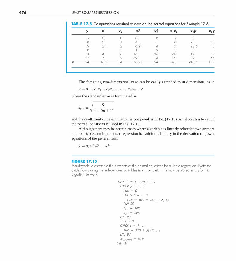
The foregoing two-dimensional case can be easily extended to m dimensions, as in

y = a0 + a1x1 + a2x2 + · · · + am xm + e

where the standard error is formulated as

sy/x =√

Sr

n − (m + 1)

and the coefficient of determination is computed as in Eq. (17.10). An algorithm to set upthe normal equations is listed in Fig. 17.15.

Although there may be certain cases where a variable is linearly related to two or moreother variables, multiple linear regression has additional utility in the derivation of powerequations of the general form

y = a0xa11 xa2

2 · · · xamm


TABLE 17.5 Computations required to develop the normal equations for Example 17.6.

y x1 x2 x12 x2

2 x1x2 x1y x2y

5 0 0 0 0 0 0 010 2 1 4 1 2 20 10

9 2.5 2 6.25 4 5 22.5 180 1 3 1 9 3 0 03 4 6 16 36 24 12 18

27 7 2 49 4 14 189 54� 54 16.5 14 76.25 54 48 243.5 100

DOFOR i � 1, order � 1DOFOR j � 1, isum � 0DOFOR � � 1, nsum � sum � xi�1,� � xj�1,�

END DOai,j � sumaj,i � sum

END DOsum � 0DOFOR � � 1, nsum � sum � y� � xi�1,�

END DOai,order�2 � sum

END DO

FIGURE 17.15Pseudocode to assemble the elements of the normal equations for multiple regression. Note thataside from storing the independent variables in x1,i, x2,i, etc., 1’s must be stored in x0,i for thisalgorithm to work.

cha01064_ch17.qxd 3/20/09 12:44 PM Page 476

Such equations are extremely useful when fitting experimental data. To use multiple linearregression, the equation is transformed by taking its logarithm to yield

log y = log a0 + a1 log x1 + a2 log x2 + · · · + am log xm

This transformation is similar in spirit to the one used in Sec. 17.1.5 and Example 17.4to fit a power equation when y was a function of a single variable x. Section 20.4 providesan example of such an application for two independent variables.

17.4 GENERAL LINEAR LEAST SQUARES

To this point, we have focused on the mechanics of obtaining least-squares fits of somesimple functions to data. Before turning to nonlinear regression, there are several issuesthat we would like to discuss to enrich your understanding of the preceding material.

17.4.1 General Matrix Formulation for Linear Least Squares

In the preceding pages, we have introduced three types of regression: simple linear, poly-nomial, and multiple linear. In fact, all three belong to the following general linear least-squares model:

y = a0z0 + a1z1 + a2z2 + · · · + am zm + e (17.23)

where z0, z1, . . . , zm are m + 1 basis functions. It can easily be seen how simple and multi-ple linear regression fall within this model—that is, z0 = 1, z1 = x1, z2 = x2, . . . , zm = xm.Further, polynomial regression is also included if the basis functions are simple monomialsas in z0 = x0 = 1, z1 = x, z2 = x2, . . . , zm = xm.

Note that the terminology “linear” refers only to the model’s dependence on itsparameters—that is, the a’s. As in the case of polynomial regression, the functions them-selves can be highly nonlinear. For example, the z’s can be sinusoids, as in

y = a0 + a1 cos(ωt) + a2 sin(ωt)

Such a format is the basis of Fourier analysis described in Chap. 19.On the other hand, a simple-looking model like

f(x) = a0(1 − e−a1x)

is truly nonlinear because it cannot be manipulated into the format of Eq. (17.23). We willturn to such models at the end of this chapter.

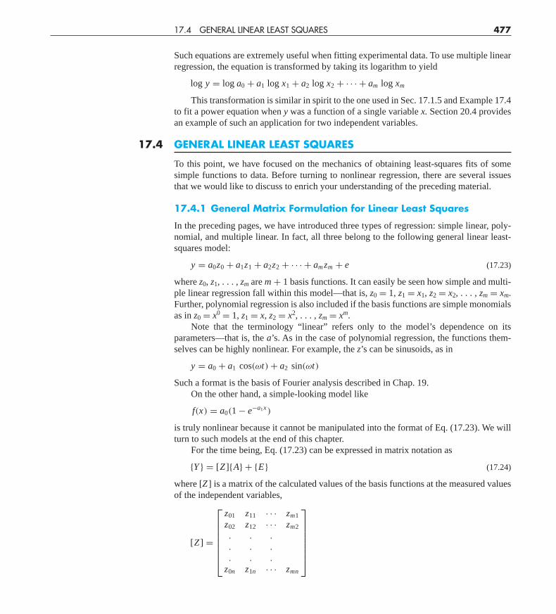
For the time being, Eq. (17.23) can be expressed in matrix notation as

{Y } = [Z ]{A} + {E} (17.24)

where [Z] is a matrix of the calculated values of the basis functions at the measured valuesof the independent variables,

[Z ] =

⎡⎢⎢⎢⎢⎢⎢⎣

z01 z11 · · · zm1

z02 z12 · · · zm2

. . .

. . .

. . .

z0n z1n · · · zmn

⎤⎥⎥⎥⎥⎥⎥⎦

17.4 GENERAL LINEAR LEAST SQUARES 477

cha01064_ch17.qxd 3/20/09 12:44 PM Page 477

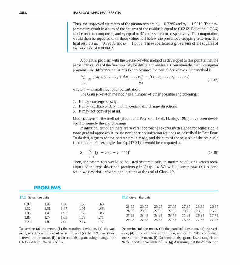
17.1 Given the data

0.90 1.42 1.30 1.55 1.631.32 1.35 1.47 1.95 1.661.96 1.47 1.92 1.35 1.051.85 1.74 1.65 1.78 1.712.29 1.82 2.06 2.14 1.27

Determine (a) the mean, (b) the standard deviation, (c) the vari-ance, (d) the coefficient of variation, and (e) the 95% confidenceinterval for the mean. (f) construct a histogram using a range from0.6 to 2.4 with intervals of 0.2.

17.2 Given the data

28.65 26.55 26.65 27.65 27.35 28.35 26.8528.65 29.65 27.85 27.05 28.25 28.85 26.7527.65 28.45 28.65 28.45 31.65 26.35 27.7529.25 27.65 28.65 27.65 28.55 27.65 27.25

Determine (a) the mean, (b) the standard deviation, (c) the vari-ance, (d) the coefficient of variation, and (e) the 90% confidenceinterval for the mean. (f) Construct a histogram. Use a range from26 to 32 with increments of 0.5. (g) Assuming that the distribution

Thus, the improved estimates of the parameters are a0 = 0.7286 and a1 = 1.5019. The newparameters result in a sum of the squares of the residuals equal to 0.0242. Equation (17.36)can be used to compute ε0 and ε1 equal to 37 and 33 percent, respectively. The computationwould then be repeated until these values fell below the prescribed stopping criterion. Thefinal result is a0 = 0.79186 and a1 = 1.6751. These coefficients give a sum of the squares ofthe residuals of 0.000662.

A potential problem with the Gauss-Newton method as developed to this point is that thepartial derivatives of the function may be difficult to evaluate. Consequently, many computerprograms use difference equations to approximate the partial derivatives. One method is

∂ fi

∂ak

∼= f(xi ; a0, . . . , ak + δak, . . . , am) − f(xi ; a0, . . . , ak, . . . , am)

δak(17.37)

where δ = a small fractional perturbation.The Gauss-Newton method has a number of other possible shortcomings:

1. It may converge slowly.2. It may oscillate widely, that is, continually change directions.3. It may not converge at all.

Modifications of the method (Booth and Peterson, 1958; Hartley, 1961) have been devel-oped to remedy the shortcomings.

In addition, although there are several approaches expressly designed for regression, amore general approach is to use nonlinear optimization routines as described in Part Four.To do this, a guess for the parameters is made, and the sum of the squares of the residualsis computed. For example, for Eq. (17.31) it would be computed as

Sr =n∑

i=1

[yi − a0(1 − e−a1xi )]2 (17.38)

Then, the parameters would be adjusted systematically to minimize Sr using search tech-niques of the type described previously in Chap. 14. We will illustrate how this is donewhen we describe software applications at the end of Chap. 19.


PROBLEMS

cha01064_ch17.qxd 3/20/09 12:44 PM Page 484

PROBLEMS 485

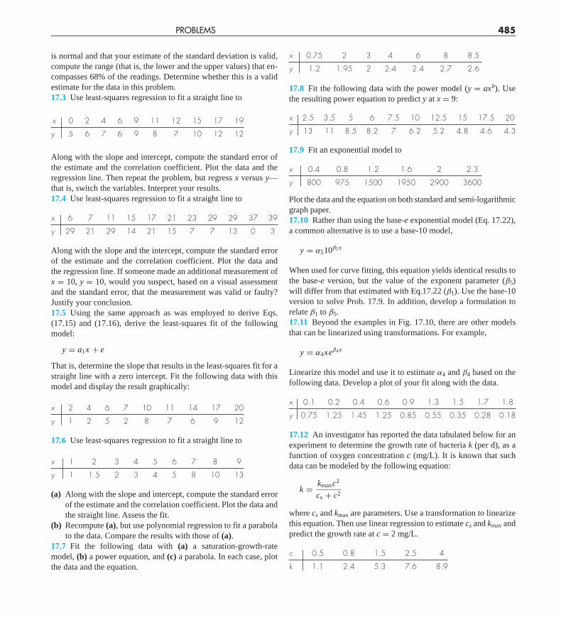
is normal and that your estimate of the standard deviation is valid,compute the range (that is, the lower and the upper values) that en-compasses 68% of the readings. Determine whether this is a validestimate for the data in this problem.17.3 Use least-squares regression to fit a straight line to

x 0 2 4 6 9 11 12 15 17 19

y 5 6 7 6 9 8 7 10 12 12

Along with the slope and intercept, compute the standard error ofthe estimate and the correlation coefficient. Plot the data and theregression line. Then repeat the problem, but regress x versus y—that is, switch the variables. Interpret your results.17.4 Use least-squares regression to fit a straight line to

x 6 7 11 15 17 21 23 29 29 37 39

y 29 21 29 14 21 15 7 7 13 0 3

Along with the slope and the intercept, compute the standard errorof the estimate and the correlation coefficient. Plot the data andthe regression line. If someone made an additional measurement ofx = 10, y = 10, would you suspect, based on a visual assessmentand the standard error, that the measurement was valid or faulty?Justify your conclusion.17.5 Using the same approach as was employed to derive Eqs.(17.15) and (17.16), derive the least-squares fit of the followingmodel:

y = a1x + e

That is, determine the slope that results in the least-squares fit for astraight line with a zero intercept. Fit the following data with thismodel and display the result graphically:

x 2 4 6 7 10 11 14 17 20

y 1 2 5 2 8 7 6 9 12

17.6 Use least-squares regression to fit a straight line to

x 1 2 3 4 5 6 7 8 9

y 1 1.5 2 3 4 5 8 10 13

(a) Along with the slope and intercept, compute the standard errorof the estimate and the correlation coefficient. Plot the data andthe straight line. Assess the fit.

(b) Recompute (a), but use polynomial regression to fit a parabolato the data. Compare the results with those of (a).

17.7 Fit the following data with (a) a saturation-growth-ratemodel, (b) a power equation, and (c) a parabola. In each case, plotthe data and the equation.

x 0.75 2 3 4 6 8 8.5

y 1.2 1.95 2 2.4 2.4 2.7 2.6

17.8 Fit the following data with the power model (y = axb). Usethe resulting power equation to predict y at x = 9:

x 2.5 3.5 5 6 7.5 10 12.5 15 17.5 20

y 13 11 8.5 8.2 7 6.2 5.2 4.8 4.6 4.3

17.9 Fit an exponential model to

x 0.4 0.8 1.2 1.6 2 2.3

y 800 975 1500 1950 2900 3600

Plot the data and the equation on both standard and semi-logarithmicgraph paper.17.10 Rather than using the base-e exponential model (Eq. 17.22),a common alternative is to use a base-10 model,

y = α510β5x

When used for curve fitting, this equation yields identical results tothe base-e version, but the value of the exponent parameter (β5)will differ from that estimated with Eq.17.22 (β1). Use the base-10version to solve Prob. 17.9. In addition, develop a formulation torelate β1 to β5.17.11 Beyond the examples in Fig. 17.10, there are other modelsthat can be linearized using transformations. For example,

y = α4xeβ4x

Linearize this model and use it to estimate α4 and β4 based on thefollowing data. Develop a plot of your fit along with the data.

x 0.1 0.2 0.4 0.6 0.9 1.3 1.5 1.7 1.8

y 0.75 1.25 1.45 1.25 0.85 0.55 0.35 0.28 0.18

17.12 An investigator has reported the data tabulated below for anexperiment to determine the growth rate of bacteria k (per d), as afunction of oxygen concentration c (mg/L). It is known that suchdata can be modeled by the following equation:

k = kmaxc2

cs + c2

where cs and kmax are parameters. Use a transformation to linearizethis equation. Then use linear regression to estimate cs and kmax andpredict the growth rate at c = 2 mg/L.

c 0.5 0.8 1.5 2.5 4

k 1.1 2.4 5.3 7.6 8.9

cha01064_ch17.qxd 3/20/09 12:44 PM Page 485

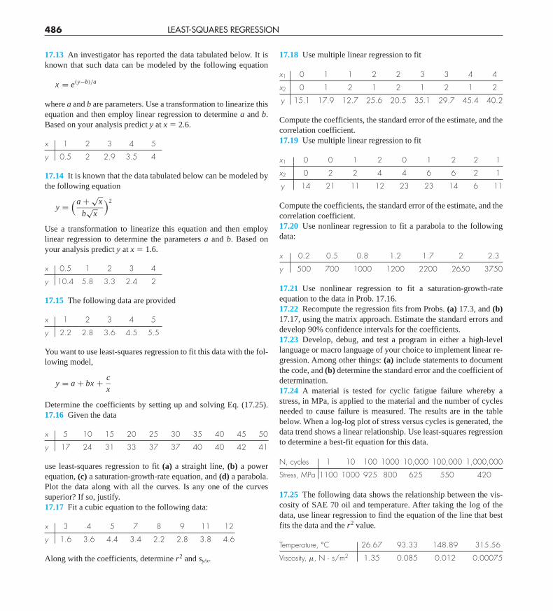
17.13 An investigator has reported the data tabulated below. It isknown that such data can be modeled by the following equation

x = e(y−b)/a

where a and b are parameters. Use a transformation to linearize thisequation and then employ linear regression to determine a and b.Based on your analysis predict y at x � 2.6.

x 1 2 3 4 5

y 0.5 2 2.9 3.5 4

17.14 It is known that the data tabulated below can be modeled bythe following equation

y =(a + √

x

b√

x

)2

Use a transformation to linearize this equation and then employlinear regression to determine the parameters a and b. Based onyour analysis predict y at x � 1.6.

x 0.5 1 2 3 4

y 10.4 5.8 3.3 2.4 2

17.15 The following data are provided

x 1 2 3 4 5

y 2.2 2.8 3.6 4.5 5.5

You want to use least-squares regression to fit this data with the fol-lowing model,

y = a + bx + c

x

Determine the coefficients by setting up and solving Eq. (17.25).17.16 Given the data

x 5 10 15 20 25 30 35 40 45 50

y 17 24 31 33 37 37 40 40 42 41

use least-squares regression to fit (a) a straight line, (b) a powerequation, (c) a saturation-growth-rate equation, and (d) a parabola.Plot the data along with all the curves. Is any one of the curvessuperior? If so, justify.17.17 Fit a cubic equation to the following data:

x 3 4 5 7 8 9 11 12

y 1.6 3.6 4.4 3.4 2.2 2.8 3.8 4.6

Along with the coefficients, determine r2 and sy/x.

17.18 Use multiple linear regression to fit

x1 0 1 1 2 2 3 3 4 4

x2 0 1 2 1 2 1 2 1 2

y 15.1 17.9 12.7 25.6 20.5 35.1 29.7 45.4 40.2

Compute the coefficients, the standard error of the estimate, and thecorrelation coefficient.17.19 Use multiple linear regression to fit

x1 0 0 1 2 0 1 2 2 1

x2 0 2 2 4 4 6 6 2 1

y 14 21 11 12 23 23 14 6 11

Compute the coefficients, the standard error of the estimate, and thecorrelation coefficient.17.20 Use nonlinear regression to fit a parabola to the followingdata:

x 0.2 0.5 0.8 1.2 1.7 2 2.3

y 500 700 1000 1200 2200 2650 3750

17.21 Use nonlinear regression to fit a saturation-growth-rateequation to the data in Prob. 17.16.17.22 Recompute the regression fits from Probs. (a) 17.3, and (b)17.17, using the matrix approach. Estimate the standard errors anddevelop 90% confidence intervals for the coefficients.17.23 Develop, debug, and test a program in either a high-levellanguage or macro language of your choice to implement linear re-gression. Among other things: (a) include statements to documentthe code, and (b) determine the standard error and the coefficient ofdetermination.17.24 A material is tested for cyclic fatigue failure whereby astress, in MPa, is applied to the material and the number of cyclesneeded to cause failure is measured. The results are in the tablebelow. When a log-log plot of stress versus cycles is generated, thedata trend shows a linear relationship. Use least-squares regressionto determine a best-fit equation for this data.

N, cycles 1 10 100 1000 10,000 100,000 1,000,000

Stress, MPa 1100 1000 925 800 625 550 420

17.25 The following data shows the relationship between the vis-cosity of SAE 70 oil and temperature. After taking the log of thedata, use linear regression to find the equation of the line that bestfits the data and the r2 value.

Temperature, °C 26.67 93.33 148.89 315.56

Viscosity, μ, N · s/m2 1.35 0.085 0.012 0.00075


cha01064_ch17.qxd 3/20/09 12:44 PM Page 486

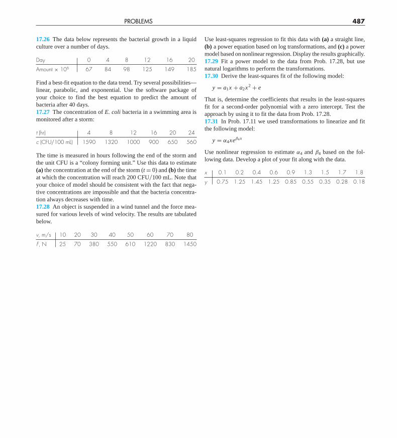
17.26 The data below represents the bacterial growth in a liquidculture over a number of days.

Day 0 4 8 12 16 20

Amount × 106 67 84 98 125 149 185

Find a best-fit equation to the data trend. Try several possibilities—linear, parabolic, and exponential. Use the software package ofyour choice to find the best equation to predict the amount ofbacteria after 40 days.17.27 The concentration of E. coli bacteria in a swimming area ismonitored after a storm:

t (hr) 4 8 12 16 20 24

c (CFU�100 mL) 1590 1320 1000 900 650 560

The time is measured in hours following the end of the storm andthe unit CFU is a “colony forming unit.” Use this data to estimate(a) the concentration at the end of the storm (t = 0) and (b) the timeat which the concentration will reach 200 CFU�100 mL. Note thatyour choice of model should be consistent with the fact that nega-tive concentrations are impossible and that the bacteria concentra-tion always decreases with time.17.28 An object is suspended in a wind tunnel and the force mea-sured for various levels of wind velocity. The results are tabulatedbelow.

v, m/s 10 20 30 40 50 60 70 80

F, N 25 70 380 550 610 1220 830 1450

Use least-squares regression to fit this data with (a) a straight line,(b) a power equation based on log transformations, and (c) a powermodel based on nonlinear regression. Display the results graphically.17.29 Fit a power model to the data from Prob. 17.28, but usenatural logarithms to perform the transformations.17.30 Derive the least-squares fit of the following model:

y = a1x + a2x2 + e

That is, determine the coefficients that results in the least-squaresfit for a second-order polynomial with a zero intercept. Test theapproach by using it to fit the data from Prob. 17.28.17.31 In Prob. 17.11 we used transformations to linearize and fitthe following model:

y = α4xeβ4x

Use nonlinear regression to estimate α4 and β4 based on the fol-lowing data. Develop a plot of your fit along with the data.

x 0.1 0.2 0.4 0.6 0.9 1.3 1.5 1.7 1.8

y 0.75 1.25 1.45 1.25 0.85 0.55 0.35 0.28 0.18

PROBLEMS 487

cha01064_ch17.qxd 3/20/09 12:44 PM Page 487

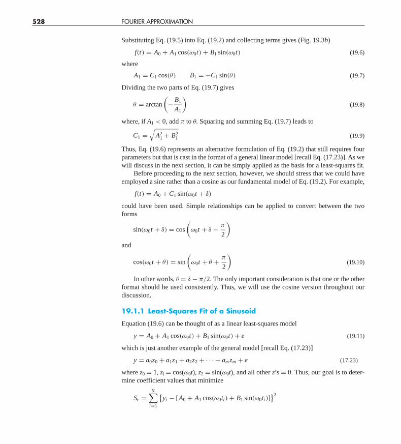
Substituting Eq. (19.5) into Eq. (19.2) and collecting terms gives (Fig. 19.3b)

f(t) = A0 + A1 cos(ω0t) + B1 sin(ω0t) (19.6)

where

A1 = C1 cos(θ) B1 = −C1 sin(θ) (19.7)

Dividing the two parts of Eq. (19.7) gives

θ = arctan

(− B1

A1

)(19.8)

where, if A1 < 0, add π to θ. Squaring and summing Eq. (19.7) leads to

C1 =√

A21 + B2

1 (19.9)

Thus, Eq. (19.6) represents an alternative formulation of Eq. (19.2) that still requires fourparameters but that is cast in the format of a general linear model [recall Eq. (17.23)]. As wewill discuss in the next section, it can be simply applied as the basis for a least-squares fit.

Before proceeding to the next section, however, we should stress that we could haveemployed a sine rather than a cosine as our fundamental model of Eq. (19.2). For example,

f(t) = A0 + C1 sin(ω0t + δ)

could have been used. Simple relationships can be applied to convert between the twoforms

sin(ω0t + δ) = cos

(ω0t + δ − π

2

)and

cos(ω0t + θ) = sin

(ω0t + θ + π

2

)(19.10)

In other words, θ = δ − π/2. The only important consideration is that one or the otherformat should be used consistently. Thus, we will use the cosine version throughout ourdiscussion.

19.1.1 Least-Squares Fit of a Sinusoid

Equation (19.6) can be thought of as a linear least-squares model

y = A0 + A1 cos(ω0t) + B1 sin(ω0t) + e (19.11)

which is just another example of the general model [recall Eq. (17.23)]

y = a0z0 + a1z1 + a2z2 + · · · + am zm + e (17.23)

where z0 = 1, zl = cos(ω0t), z2 = sin(ω0t), and all other z’s = 0. Thus, our goal is to deter-mine coefficient values that minimize

Sr =N∑

i=1

{yi − [A0 + A1 cos(ω0ti ) + B1 sin(ω0ti )]

}2

528 FOURIER APPROXIMATION

cha01064_ch19.qxd 3/20/09 12:51 PM Page 528

19.1 CURVE FITTING WITH SINUSOIDAL FUNCTIONS 529

The normal equations to accomplish this minimization can be expressed in matrix form as[recall Eq. (17.25)]⎡

⎣ N � cos(ω0t) � sin(ω0t)� cos(ω0t) � cos2(ω0t) � cos(ω0t) sin(ω0t)� sin(ω0t) � cos(ω0t) sin(ω0t) � sin2(ω0t)

⎤⎦

⎧⎨⎩

A0

A1

B1

⎫⎬⎭

=⎧⎨⎩

�y�y cos(ω0t)�y sin(ω0t)

⎫⎬⎭ (19.12)

These equations can be employed to solve for the unknown coefficients. However,rather than do this, we can examine the special case where there are N observations equi-spaced at intervals of �t and with a total record length of T = (N − 1) �t. For this situa-tion, the following average values can be determined (see Prob. 19.3):

� sin(ω0t)

N= 0

� cos(ω0t)

N= 0

� sin2(ω0t)

N= 1

2

� cos2(ω0t)

N= 1

2(19.13)

� cos(ω0t) sin(ω0t)

N= 0

Thus, for equispaced points the normal equations become⎡⎣ N 0 0

0 N/2 00 0 N/2

⎤⎦

⎧⎨⎩

A0

A1

B1

⎫⎬⎭ =

⎧⎨⎩


⎫⎬⎭

The inverse of a diagonal matrix is merely another diagonal matrix whose elements are thereciprocals of the original. Thus, the coefficients can be determined as⎧⎨

⎩A0

A1

B1

⎫⎬⎭ =

⎡⎣ 1/N 0 0

0 2/N 00 0 2/N

⎤⎦

⎧⎨⎩


⎫⎬⎭

or

A0 = �y

N(19.14)

A1 = 2

N�y cos(ω0t) (19.15)

B1 = 2

N�y sin(ω0t) (19.16)

EXAMPLE 19.1 Least-Squares Fit of a Sinusoid

Problem Statement. The curve in Fig. 19.3 is described by y = 1.7 + cos(4.189t +1.0472). Generate 10 discrete values for this curve at intervals of �t = 0.15 for the range

cha01064_ch19.qxd 3/20/09 12:51 PM Page 529

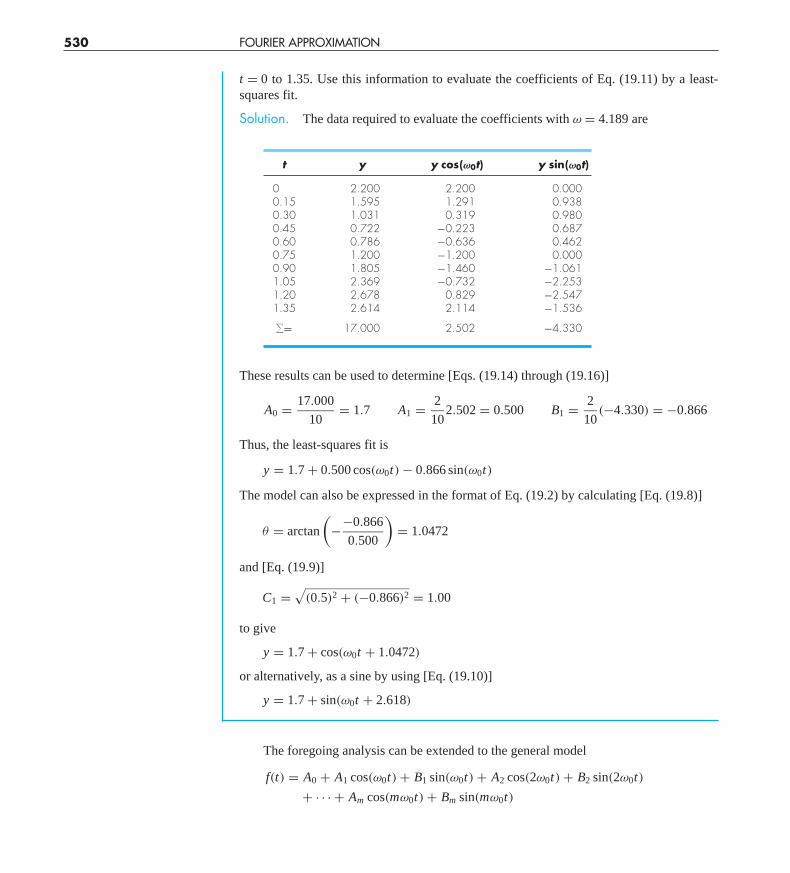
t = 0 to 1.35. Use this information to evaluate the coefficients of Eq. (19.11) by a least-squares fit.

Solution. The data required to evaluate the coefficients with ω = 4.189 are

t y y cos(ωω0t) y sin(ωω0t)

0 2.200 2.200 0.0000.15 1.595 1.291 0.9380.30 1.031 0.319 0.9800.45 0.722 −0.223 0.6870.60 0.786 −0.636 0.4620.75 1.200 −1.200 0.0000.90 1.805 −1.460 −1.0611.05 2.369 −0.732 −2.2531.20 2.678 0.829 −2.5471.35 2.614 2.114 −1.536

�= 17.000 2.502 −4.330

These results can be used to determine [Eqs. (19.14) through (19.16)]

A0 = 17.000

10= 1.7 A1 = 2

102.502 = 0.500 B1 = 2

10(−4.330) = −0.866

Thus, the least-squares fit is

y = 1.7 + 0.500 cos(ω0t) − 0.866 sin(ω0t)

The model can also be expressed in the format of Eq. (19.2) by calculating [Eq. (19.8)]

θ = arctan

(−−0.866

0.500

)= 1.0472

and [Eq. (19.9)]

C1 =√

(0.5)2 + (−0.866)2 = 1.00

to give

y = 1.7 + cos(ω0t + 1.0472)

or alternatively, as a sine by using [Eq. (19.10)]

y = 1.7 + sin(ω0t + 2.618)

The foregoing analysis can be extended to the general model

f(t) = A0 + A1 cos(ω0t) + B1 sin(ω0t) + A2 cos(2ω0t) + B2 sin(2ω0t)

+ · · · + Am cos(mω0t) + Bm sin(mω0t)

530 FOURIER APPROXIMATION

cha01064_ch19.qxd 3/20/09 12:51 PM Page 530

19.2 CONTINUOUS FOURIER SERIES 531

where, for equally spaced data, the coefficients can be evaluated by

A0 = �y

N

Aj = 2

N�y cos( jω0t)

Bj = 2

N�y sin( jω0t)

⎫⎪⎬⎪⎭ j = 1, 2, . . . , m

Although these relationships can be used to fit data in the regression sense (that is,N > 2m + 1), an alternative application is to employ them for interpolation or colloca-tion—that is, to use them for the case where the number of unknowns, 2m + 1, is equal tothe number of data points, N. This is the approach used in the continuous Fourier series, asdescribed next.

19.2 CONTINUOUS FOURIER SERIES

In the course of studying heat-flow problems, Fourier showed that an arbitrary periodicfunction can be represented by an infinite series of sinusoids of harmonically related fre-quencies. For a function with period T, a continuous Fourier series can be written1

f(t) = a0 + a1 cos(ω0t) + b1 sin(ω0t) + a2 cos(2ω0t) + b2 sin(2ω0t) + · · ·or more concisely,

f(t) = a0 +∞∑

k=1

[ak cos(kω0t) + bk sin(kω0t)] (19.17)

where ω0 = 2π/T is called the fundamental frequency and its constant multiples 2ω0, 3ω0,etc., are called harmonics. Thus, Eq. (19.17) expresses f (t) as a linear combination of thebasis functions: 1, cos(ω0t), sin(ω0t), cos(2ω0t), sin(2ω0t), . . . .

As described in Box 19.1, the coefficients of Eq. (19.17) can be computed via

ak = 2

T

∫ T

0f(t) cos(kω0t) dt (19.18)

and

bk = 2

T

∫ T

0f(t) sin(kω0t) dt (19.19)

for k = 1, 2, . . . and

a0 = 1

T

∫ T

0f(t) dt (19.20)

1The existence of the Fourier series is predicated on the Dirichlet conditions. These specify that the periodic func-tion have a finite number of maxima and minima and that there be a finite number of jump discontinuities. In gen-eral, all physically derived periodic functions satisfy these conditions.

cha01064_ch19.qxd 3/20/09 12:51 PM Page 531

least-squares regressiondewan.buet.ac.bd/eee423/coursematerials/curve-fitting.pdf · are met,...

Documents