least squares moving particle semi-implicit method · least squares moving particle semi-implicit...

Comp. Part. Mech. (2014) 1:277–305DOI 10.1007/s40571-014-0027-2

Least squares moving particle semi-implicit methodAn arbitrary high order accurate meshfree Lagrangian approach for incompressible flowwith free surfaces

Tasuku Tamai · Seiichi Koshizuka

Received: 27 February 2014 / Revised: 8 May 2014 / Accepted: 26 May 2014 / Published online: 11 July 2014© OWZ 2014

Abstract In this paper, a consistent meshfree Lagrangianapproach for numerical analysis of incompressible flowwith free surfaces, named least squares moving particlesemi-implicit (LSMPS) method, is developed. The presentmethodology includes arbitrary high-order accurate mesh-free spatial discretization schemes, consistent time integra-tion schemes, and generalized treatment of boundary condi-tions. LSMPS method can resolve the existing major issues ofwidely used strong-form particle method for incompressibleflow—particularly, the lack of consistency condition for spa-tial discretization schemes, difficulty in enforcing consistentNeumann boundary conditions, and serious instability likeunphysical pressure oscillation. Applications of the presentproposal demonstrate remarkable enhancements of stabilityand accuracy.

Keywords Least squares moving particle semi-implicitmethod · LSMPS method · High order scheme · Meshfreecompact scheme · Moving particle semi-implicit method

1 Introduction

Today the finite element method (FEM) [101], the finite vol-ume method (FVM) [98], and the finite difference method(FDM) [87] based computational mechanics play a conspic-uous role in technology advancement. A noteworthy featureof them is that they divide a continuum domain into discretesubdivision usually called mesh/grid, which requires connec-

T. Tamai (B) · S. KoshizukaGraduate School of Engineering, The University of Tokyo,7-3-1,Hongo, Bunkyo-ku, Tokyo 113-8656, Japane-mail: [email protected]

S. Koshizukae-mail: [email protected]

tivity based on a topological map; however, the characteris-tic of them is not always suitable. For instance, in order toadapt topological and geometric changes undergone by thereal material, such as simulations of fluid flow or large straincontinuum deformation, Lagrangian description (i.e. movingmesh/grid) could be applied; however, one would face dis-tortion of mesh/grid which results in either termination of thecomputation or severe deterioration in numerical accuracy.Arbitrary Lagrangian Eulerian (ALE) formulations [26,36]have been developed to overcome the difficulty caused bydistortion of mesh/grid, of which objective is to move mesh/grid independently from actual motion of material so that dis-tortion could be minimized; nevertheless, distortion of mesh/grid still remains and causes overwhelming errors in numer-ical solutions.

Under these circumstances, meshfree methods and/or par-ticle methods, which discretize a continuum by only a set ofnodal points or particles, have been sought in order to find bet-ter discretization procedures without mesh/grid constraints.Since the connectivity among nodes can be generated any-time desired and can change with time, meshfree/particlemethods can easily handle simulations of very large defor-mations, even with the changes of the topological structureand fragmentation–coalescence of continuum.

In general, according to computational modelings and for-mulations, meshfree/particle methods can be categorized intotwo different classifications as well: the weak form formula-tions of Partial Differential Equations (PDEs); and the strongform formulations of PDEs. The first class of meshfree/particle methods is used with various weak formulations suchas Galerkin methods, for example, diffuse element method(DEM) [73], element free Gelerkin (EFG) method [11,13–15,67], reproducing Kernel particle method (RKPM) [21,63–65], h-p cloud method [27,28,58,74], partition of unitymethod (PUM) [7–9,69], meshless local Petrov–Gelerkin

123

278 Comp. Part. Mech. (2014) 1:277–305

(MLPG) method [2–6], finite point method (FPM) [75–77,80], particle finite element method (P-FEM) [38,78,79],reproducing Kernel element method (RKEM) [56,62,66,86].The second category of meshfree/particle methods is usedto approximate the strong form PDEs discretized by spe-cific collocation techniques, for instance, smoothed parti-cle hydrodynamics (SPH) method [31,60,68,71,72], movingparticle semi-implicit (MPS) method [48,49], meshfree finitedifference method [57,59], finite pointset method (FPM)[95–97].

In various weak form meshfree/particle methods, shapefunctions, or more general meshfree interpolants, are con-structed based on the so-called “partition of unity”, then con-sistency conditions, polynomial completeness, or reproduc-ing conditions are satisfied. On the other hand, although thestrong form particle methods such as the SPH method and theMPS method have been shown to be useful widely in engi-neering applications especially in fluid dynamics, their stan-dard formulae of spatial discretization schemes are not con-sistent except under very limited conditions, and do not holdpolynomial completeness/reproducing conditions or differ-ential completeness/reproducing conditions. According tothe Lax’s equivalence theorem [51], this major issue mustnever be overlooked. Moreover, this matter yields adverseeffects for both computational accuracy and stability. Somecorrection methods for resolving the lack of polynomial com-pleteness or reproducing conditions on the spatial discretiza-tion schemes (which will be discussed in Chap. 3) have beenproposed; however, they are far from adequate in terms ofthe compatibility with satisfaction of higher order consis-tency conditions and numerical stability. Strong form mesh-free/particle methods still have a difficulty relating to pro-cedures of enforcing boundary conditions, especially Neu-mann boundary conditions. Hence, prevailing strong formparticle methods, whose advantage is that they can hand-ily run numerical analysis of continuum with large defor-mation, even with the changes of topological structure andfragmentation–coalescence, are inadequately studied as anaccurate mathematical computation.

With taking particular note to controversies describedabove, we develop a new consistent fully Lagrangian mesh-free particle method, named least squares moving particlesemi-implicit (LSMPS) method, for numerical analysis ofincompressible fluid flow with free surfaces. As its name sug-gests, LSMPS method is based on the method of weighted“Least Squares” procedure, and follows fundamentals of theMPS method [48,49]: “Moving Particle” means meshfreefully Lagrangian approach, and “Semi-implicit” representsthe type of time integration algorithm for incompressible flowwhich is well-known as the projection method [33]. LSMPSmethod succeeds the name of the existing MPS method; how-ever, all of LSMPS formulae are different from of the currentMPS method.

In this paper, we introduce a new methodology and for-mulae as a meshfree Lagrangian approach (particle method),including arbitrary high order accurate meshfree spatial dis-cretization schemes, consistent time integration schemes, andgeneralized treatment of boundary conditions. Additionally,some numerical demonstrations compared with the conven-tional MPS solutions show drastic improvement of accuracyand stability.

2 Preliminary

2.1 Notation

In order to expedite the presentation, we introduce some pre-liminaries for notations. Throughout this paper, the letter d isa positive integer and denotes the spatial dimension. Ω ⊆ R

d

is a nonempty, open, bounded, and connected set. ∂Ω denotesthe boundary of Ω , and ∂Ω is assumed to be Lipschitz con-tinuous or smoother, as the case may be.

N0 denotes the set of non negative integers. If

α := (α1, α2, . . . , αd) ∈ Nd0 (1)

is an d-tuple of non negative integers, we call α a multi-index.Then, the quantity

|α| :=d∑

i=1

αi , (2)

is defined to be the length of α. We also use the followingconventions:

α! := α1! . . . αd !, ∀α ∈ Nd0 . (3)

If α,β ∈ Nd0 , we say β ≤ α provided

1 ≤ ∀i ≤ d, βi ≤ αi . (4)

By the same token,(

α

β

):= α!

β!(α − β)! =(

α1

β1

). . .

(αd

βd

). (5)

If x := (x1, . . . , xd)T ∈ Rd and α ∈ N

d0 , then xα is

defined as follows:

xα := xα11 · · · xαd

d . (6)

If f (x) is a real valued function on an open subset of Rd , α ∈

Nd0 and smoothness of f is assumed enough, then Dα

x f (x)

denotes the αth order Fréchet derivative of f as follows:

Dαx f (x) := ∂ |α| f (x)

∂xα11 · · · ∂xαd

d

. (7)

123

Comp. Part. Mech. (2014) 1:277–305 279

If x = (x1, . . . , xd)T is an arbitrary point of Rd , then

‖x‖2 =√√√√

d∑

i=1

x2i (8)

denotes the Euclidian norm of x, and we usually use ‖x‖ asabridged notation.

2.2 Consistency, completeness, reproducing condition, andthe partition of unity

In order to advance concrete discussions on the study of con-vergence, according to Belytschko et al. [12], three terms arefrequently used: (i) Consistency [90] : a property of the dis-cretization schemes for partial differential equations, whichis usually utilized in Finite Difference approximations, (ii)Reproducing conditions [64,65]: the ability of the approxi-mation to reproduce specified functions, which are usuallypolynomials, (iii) Completeness [37]: polynomial complete-ness or completeness , which is usually discussed in the FEM.

2.2.1 Consistency

Strikwerda [90] defines the consistency condition of partic-ular operators for approximating derivatives as follows:

Theorem 2.1 (Consistency [12,90]) A scheme Lhu = fthat is consistent with the differential equation Lu = f isaccurate (consistent) of order p if for any sufficiently smoothfunction v

Lv − Lhv = O(h p) (9)

In the above definition, a parameter h denotes the refinementof mesh/grid and p refers to the order of consistency. Obvi-ously, it is necessary for convergence that p > 0, and werequire that p ≥ 1 for the efficient numerical calculation.

According to the well-known Lax-Richtmyer equivalencetheorem [51], a consistent finite difference scheme for a well-posed partial differential equation is convergent if and onlyif it is stable. Consequently, any discretization scheme mustsatisfy the pth order (p > 0) consistency condition to obtainconvergence. The consistency is straightforward to verify andstability is typically much easier to show than convergence;therefore, the convergence is usually studied via the Lax-Richtmyer equivalence theorem.

2.2.2 Completeness, reproducing condition, and thepartition of unity–nullity

Since ascertaining whether meshfree interpolants are consis-tent for irregularly distributed nodes is significantly more dif-ficult than examining whether finite difference schemes fora uniform structured grid, the completeness or reproducing

conditions which play the same role [12] as the consistencyconditions1 are explored, instead.

The reproducing conditions or the completeness are theability of the approximation to reproduce specified functionswhich are usually polynomials. One can say that an approxi-mation f h(x) is complete to order p if any given polynomialup to order p can be reproduced exactly. If an approximationf h(x) is given by

f h(x) =∑

i

Φi (x) f (xi ), (10)

where {Φi (x)}1≤i≤N are the interpolant functions and{ f (xi )}1≤i≤N are given nodal values for the set of nodes{xi }1≤i≤N , then the completeness or the reproducing condi-tions can be defined as follows:

Theorem 2.2 (pth order completeness/reproducing condi-tion) For a multi index α ∈ N

d0 : 0 ≤ |α| ≤ p, an interplant

function Φi (x) ∈ R holds the pth order polynomial com-pleteness/reproducing condition if it satisfies:∑

i

(x − xi )αΦi (x) = δα0, (11)

or equivalently,∑

i

xαi Φi (x) = xα. (12)

Some meshfree discretization schemes are formulated tosatisfy alternatives, the differential completeness or the dif-ferential reproducing conditions which are requirement thatthe derivatives of a polynomial field be reproduced correctly.They can be defined directly from Theorem 2.2 by takingderivatives of Eqs. (11) and (12), i.e.

Theorem 2.3 (pth order differential completeness/reproducing condition) Let an interplant function Φi (x) ∈Ck(Rd). For multi indicies α,β ∈ N

d0 : 0 ≤ |α| ≤ p, 0 ≤

|β| ≤ k(≤ p), an interplant function Φi (x) holds the pthorder differential completeness/reproducing condition if itsatisfies:∑

i

(x − xi )α Dβ

x Φi (x) = (−1)|β|α!δαβ , (13)

or equivalently,

∑

i

xαi Dβ

x Φi (x) = α!(α − β)!xα−β . (14)

It should be noted that the Theorem 2.2 and 2.3 are simi-lar to pth order consistency condition and pth order differen-tial consistency condition for RKPM shape function [55,65],respectively.

1 pth order polynomial completeness conditions or reproducing condi-tions is sufficient condition of pth order consistency.

123

280 Comp. Part. Mech. (2014) 1:277–305

If α = 0, Eqs. (11) and (12) become∑

i

Φi (x) = 1, (15)

and if α �= 0, Eq. (11) does∑

i

(x − xi )αΦi (x) = 0. (16)

These are the origin of the name “The Partition of Unity”,and “The Partition of Nullity”. These properties are closelyrelated with not only meshfree interpolant [65] but alsomesh-based one. Obviously, since FEM interpolant func-tions, called shape functions satisfy the Kronecker delta prop-erty, they are constructed based on the partition of unity–nullity. Moreover, weighting coefficients of linear combina-tion on the finite difference schemes are built on the partitionof unity–nullty to obtain certain order of consistency.

Interestingly, Liu et al. [65] showed that least squaresbased interpolants provide achievement of polynomial com-pleteness/reproducing conditions, or so-called the partitionof unity–nullity—vice versa, corrected interpolant formulaeto fulfill the polynomial completeness/reproducing condi-tions are quite identical to the production derived from leastsquares procedures. Chakravarthy [17] showed the funda-mental concept of the finite difference schemes that to deter-mine unknowns emerged from Taylor expansion or poly-nomial approximation is generalization of finite differenceoperator. Also, it yields normal equations which is the veryidea of the linear least squares approaches.

With focusing attention to a close relationship of consis-tency, completeness/reproducing conditions, and the parti-tion of unity–nullity, and leveraging the fact that the leastsquares schemes contribute achievement of arbitrary high-order consistency conditions for meshfree spatial discretiza-tion schemes, we develop new formulae in the next section.

3 Meshfree spatial discretization schemes

3.1 An overview of the existing meshfree spatialdiscretization schemes

As mentioned it in the introduction, various meshfree and/orparticle methods have been sought, in order to discretize adomain without mesh/grid constraints. There are a lot of dis-cretization schemes for meshfree interpolants and meshfreefinite difference. One of the most prevalent particle meth-ods is the SPH method which discretizes partial differentialequations by a integral representation collocation technique.Even though the SPH method has achieved a lot of successin computational mechanics, it has not been viewed as anaccurate mathematical computation which stems from the

fact that it lacks a rigorous convergence theory as well as asuccessive refinement procedure [81].

The early SPH interpolants do not satisfy the discrete par-tition of unity and nullity [63] except under very limited con-ditions. This means the defection of SPH interpolants 0th orhigher order completeness/reproducing conditions in generalparticle distribution, which results in incapability of repre-senting rigid body motion correctly, even though it is Galileaninvariant (rigid body translation only). Also, the primal SPHgradient operator and Laplace operator generally have analo-gous problem. In order to solve this matter, several correctionschemes have been proposed, for example, Monaghan’s sym-metrization on derivative approximation [70,71], Johnson–Beissel correction [41], Randles–Libersky correction [82],Krongauz–Belytschko correction [12], Chen–Beraun cor-rection [18–20], Bonet-Kulasegaram integration correction[16], Aluru’s collocation RKPM [1], Zhang–Batra correction[99,100]. They correct SPH kernel interpolant to satisfy com-pleteness/reproducing condition in the interpolation field, orequivalently, to modify SPH derivative approximation oper-ators directly to meet derivative completeness/reproducingcondition in the derivative of the interpolants. It must be men-tioned that almost all 1st or higher order consistent correctedformulae as listed above are based on the least squares meth-ods, for instance, the most widely used 1st order consistentgradient approximation operator for the SPH method devel-oped by Randles–Libersky [82] is one of the least squaresbased discretizations.

Least squares procedures are excellent with meshfreeinterpolants or meshfree finite difference schemes. Liu etal. [65] demonstrate that moving least squares (MLS) [50]approximation is equivalent to reproduced Kernel (RK)interpolant [65] which are corrected kernel approximationbased on the reproducing conditions. MLSRK interpolantcan provide arbitrary high order consistency condition, andis the contemporary version of the classical MLS one sincethe basic concept of reproducing kernel, or more gener-ally speaking, the fundamentals of the partition of unity–nullity incubates various derivation of meshfree interpolants[54,61,62] . With taking particular note of the SPH kernelinterpolant inconsistency, Dilts [24,25] utilizes MLS inter-polant [50] to improve the accuracy of the SPH kernel approx-imation, so-called moving least squares particle hydrody-namics (MLSPH). Since MLS can construct sufficientlysmoothed interpolation globally with optional order of poly-nomial completeness/reproducing conditions, it is widelyused in meshfree/particle methods, such as various Galerkinmeshfree approach listed in Introduction (e.g. DEM, EFGM,RKPM, etc. ).

Since the early MPS gradient operator and Laplace oper-ator [49] generally lack 1st or higher order differential com-pleteness/reproducing condition except under very limitedconditions (e.g. regular particle distribution is assumed),

123

Comp. Part. Mech. (2014) 1:277–305 281

varied correction techniques have been proposed in orderto enhance the accuracy of the MPS method. For instance,Khayyer–Gotoh gradient operator anti-symmetrization [42],Khayyer–Gotoh divergence operator correction [43],Khayyer–Gotoh Laplace operator correction [44], Khayyer–Gotoh gradient operator correction [45], and Suzuki gradi-ent operator correction [39,91] are proposed. Only Suzukimethod based on weighted least squares technique canachieve 1st order consistency for gradient operator; however,others do not hold differential completeness/reproducingconditions in general case. In other words, they are farfrom satisfaction of high order accuracy. Of course, sim-ilar to adopting least squares approach into SPH method,least squares based formulae can be introduced to the MPSmethod. Koh et al. [46] utilize two dimensional secondorder generalized finite difference schemes [57,59] basedon weighted least squares to the MPS method. Tamai et al.[93] formulate generalized finite difference schemes basedon the weighted least squares for the MPS method, whichprovides arbitrary high order consistency and can be appliedfor arbitrary dimension.

Consistent least squares based spatial discretization finitedifference schemes [46,57,59,91,93] resolve the rack ofpolynomial completeness/reproducing conditions on theMPS method so that high order consistency conditionsare fulfilled and absolute enhancement of accuracy wouldbe given; however, utilizing least squares based schemeraise a new problem—normal equations derived from theleast squares procedures will be ill-conditioned problemswhich results in either serious deterioration in numericalaccuracy and stability or termination of the computation.Selecting neighborhood stenciles [59] to circumvent this ill-conditioned problems is proposed; however, this techniquecan not be the fundamental solution since the condition num-bers of coefficient matrices derived from the least squares,so-called the “moment matrices”, are not independent fromcharacteristic length of calculation points spacing.

In order to overcome the weakness of the least squaresbased spatial discretization schemes that normal equationsshall be ill-conditioned and to obtain high order consistencyconditions from them, we reformulate the least squares basedschemes in the next section.

3.2 A new meshfree spatial discretization schemes based onthe weighted least squares procedure

3.2.1 Stone–Weierstrass theorem of locally compact version

Let f : Rd → R be a sufficiently smooth function2 that is

defined on a simply connected open set Ω ⊆ Rd . Accord-

ing to the Stone-Weirestrass theorem of locally compact ver-

2 At least, f (x) ∈ C0(Ω).

sion [84,88,89], for a fixed point x ∈ Ω , one should alwaysbe able to approximate f (x) by a polynomial series locally.Thus, we can define a local function

f l(x, x) :={

f (x), ∀x ∈ B(x),

0, ∀x �∈ B(x),(17)

where

B(x) :={

x∣∣∣ ‖x − x‖ < re, x ∈ R

d}

. (18)

If the function f (x) is smooth enough as assumed, thereexists a local operator L x : C0(B(x)) → C p(B(x)) s.t.

f l(x, x) ≈ L x f (x) := pT (x)a(x), (19)

where

p(x) :={

xα∣∣∣ 0 ≤ |α| ≤ p

}, (20)

is pth order complete polynomial basis, and a(x) is coef-ficient vector. Utilizing Taylor expansion of approximatedpolynomial function around xi with nearby point x j ∈ B(x)

yields

p∑

|α|=1

[1

α!(x j − xi

)αDα

x f h(xi )

]

− { f (x j ) − f (xi )} = R p+1i j , (21)

where

R p+1i j := L x f (x) − f l(x), (22)

is the residual of local polynomial approximation. Equation(21) is a well-known form of Taylor expansion, and we useit several times in this paper without special note again.

3.2.2 Weight function

We use the weighted least squares procedures for new spatialdiscretization schemes formulae, then the weight(window)function which satisfy the following conditions is defined.

w(x, re) ∈ Ck0 (Rd), 1 ≤ k, (23)

∀x ∈ Rd , 0 ≤ w(x, re) ≤ Cw < ∞, (24)

‖x‖ ≥ re ⇐⇒ w(x, re) = 0, (25)

‖x‖ < ‖y‖ ≤ re �⇒ w(x, re) > w(y, re), (26)∫

Rd

w(x, re)dx=C =(Const.), (Typically, C =1), (27)

where re is the dilation parameter and the radius of com-pact support of the weight function. In the LSMPS method,singular weight function like

123

282 Comp. Part. Mech. (2014) 1:277–305

w(x, re) =⎧⎨

⎩

re

‖x‖ − 1, 0 ≤ ‖x‖ < re,

0, re ≤ ‖x‖,(28)

which is usually used in the MPS method, could be applied;therefore, the condition of non-singularity (Eq. 24) is not nec-essarily for the weight function. For obtaining stable calcula-tion, however, application of non-singular weight functionsis highly recommended.

3.2.3 Standard scheme type-A

We define new meshfree spatial discretization schemes witharbitrary high order consistency conditions.

Definition 3.1 (Standard LSMPS scheme, Type-A) Letf : R

d → R be a sufficiently smooth function on asimply connected open set Ω ⊂ R

d . Standard LSMPSschemes type-A are defined as follows:

Dx f h(xi ) := Hrs

[M−1

i bi

](29)

where

Dx := {Dα

x | 1 ≤ |α| ≤ p}, (30)

Hrs := diag

{{rs

−|α|α!}

1≤|α|≤p

}, (31)

Mi :=∑

j∈Λi

[w

(‖x j − xi‖re

)

p(

x j − xi

rs

)pT(

x j − xi

rs

)],

(32)

bi :=∑

j∈Λi

[w

(‖x j − xi‖re

)

p(

x j − xi

rs

){ f (x j ) − f (xi )}

],

(33)

p (x) := {xα | 1 ≤ |α| ≤ p

}, (34)

Λi :={

j∣∣∣ 0 ≤ ‖x j − xi‖ < re

}(35)

re : dilation parameter (0 < re),

rs : scaling parameter (0 < rs ≤ re).

p : order of polynomial basis

Derivation:According to the Stone–Weierstrass theorem discussed in

the Sect. 3.2.1, and utilizing Taylor expansion of local poly-nomial approximation, one can obtain

p∑

|α|=1

[1

α!(x j −xi

)αDα

x f h(xi )

]−{ f (x j )− f (xi )}= R p+1

i j .

(36)

If we use weighted least squares technique to minimizeweighted squared residuals

∑

j∈Λi

wi j

(R p+1

i j

)2,

associated with the residual R p+1i j and weight function wi j ,

normal equations equivalent to the existing spatial dis-cretization formulae [59,93] based on the weighted leastsquares procedure are provided; however, they must be ill-conditioned if p ≥ 2 as discussed in Sect. 3.1. In order to fixthis issue, we now introduce adroit variable transformationfor unknowns s.t.

Dαx f h(xi ) −→ r |α|

s

α! Dαx f h(xi ), (37)

where rs : 0 < rs ≤ re is the scaling parameter, then Eq.(36) can be equivalently transformed into

p∑

|α|=1

[{(x j − xi

)α

r |α|s

}{r |α|

s

α! Dαx f h(xi )

}]

−{ f (x j ) − f (xi )} = R p+1i j . (38)

One can transliterate this equation with symbols Dx, Hrs ,

p(x) defined by Eqs. (30), (31), and (34),

pT(

x j −xi

rs

){H−1

rsDx f h(xi )

}−{ f (x j )− f (xi )} = R p+1

i j ,

(39)

and applicate the weighted least squares procedures. If wedefine a discrete functional associated with R p+1

i j ,

J (H−1rs

Dx f h(xi ))

:=∑

j∈Λi

w

(‖x j − xi‖re

)(R p+1

i j

)2(40)

=∑

j∈Λi

w

(‖x j − xi‖re

)

[pT(

x j −xi

rs

){H−1

rsDx f h(xi )

}−{ f (x j )− f (xi )}

]2

,

(41)

123

Comp. Part. Mech. (2014) 1:277–305 283

normal equations can be provided by minimizing functionalJ , i.e.

⎡

⎣∑

j∈Λi

w

(‖x j − xi‖re

)p(

x j − xi

rs

)pT(

x j − xi

rs

)⎤

⎦

·{

H−1rs

Dx f h(xi )}

=⎡

⎣∑

j∈Λi

w

(‖x j − xi‖re

)p(

x j − xi

rs

)( f (x j ) − f (xi ))

⎤

⎦ .

(42)

One can transliterate the above with symbols Mi , bi

defined by Eqs. (32) and (33),

Mi

{H−1

rsDx f h(xi )

}= bi . (43)

Thus, if the moment matrix Mi is not singular, solutionsH−1

rsDx f h(xi ) are uniquely determined by solving normal

equations,

H−1rs

Dx f h(xi ) = M−1i bi . (44)

Finally, since the scaling matrix HrS defined by Eq. (31) isalways non-singular and invertible, we can obtain the Stan-dard LSMPS scheme formulae type-A,

Dx f h(xi ) = Hrs [M−1i bi ]. (45)

Remark 3.2 Introducing scaling for the basis is not a brandnew technique since MLSRK interpolant [65] alreadyinstalled it; however, it must be mentioned that there exists aconcrete difference. MLSRK basis utilizes dilation parame-ter (= re) for scaling the basis. On the other hand, LSMPSformulae employs another parameter rs : 0 < rs ≤ re =

for scaling. This minor change results in major alterationin the condition number of moment matrices, which will beinvestigated in later.

Since the standard LSMPS schemes type-A are derivedfrom the weighted least squares method, heritages from thepast studies related to the least squares one could be applied.

Definition 3.3 ((re, p)-regularity on the standard LSMPSscheme type-A) A family of particle distribution {xi }1≤i≤N

is said to be (re, p)-regular, if there exists a constant C s.t.

∀xi ∈ Ω, maxxi ∈Ω

‖M−1i ‖ ≤ C (46)

When {xi }1≤i≤N is (re, p)-regular, the condition numberof Mi , which is equal to ‖Mi‖‖M−1

i ‖ will be uniformlybounded. It must be mentioned that the definition of (re, p)-regularity above is nearly accordance with the concept of(, p)-regularity, which has been introduced by Han andMeng [34] for the RKPM.

Definition 3.4 (Admissible particle distribution on the stan-dard LSMPS scheme type-A) For a given particle distribution{xi }1≤i≤N , let B(x, r) := {

x′ ∈ Rd | ‖x − x′‖ ≤ r

}, fill dis-

tance : hx,Ω := supx∈Ω

min1≤i≤N

‖x − xi‖, and separation distance

: ηx := 12 min

j �=i‖x j −xi‖, then admissible particle distribution

on the standard scheme type-A is defined as follows:

Ω ⊂N⋃

i=1

B(xi , hx,Ω/2), (47)

card{xα∣∣ 1 ≤ |α| ≤ p

}

≤ card{

j∣∣ x j ∈ B(xi , chx,Ω)

}, c ≥ 1,∀ i, (48)

∃δ > 0 s.t. ηx ≤ hx,Ω ≤ δηx. (49)

Theorem 3.5 (Consistency of the Standard LSMPS schemetype-A) Let f : R

d → R be a sufficiently smooth functionthat is defined on a open set Ω ⊂ R

d , and assume thatf (x) ∈ C p+1(Ω). For multi-index α : 1 ≤ |α| ≤ p, thereexists a constant C : 0 ≤ C < ∞, then Standard LSMPSscheme type-A holds the following consistency condition.

|Dαx f (x) − Dα

x f h(x)| ≤ Cr p+1−|α|e | f (x)|C p+1(Ω) (50)

Proof Utilizing Taylor expansion of f (x) ∈ C p+1(Ω)

yields

f (x j ) =p∑

|α|=0

[1

α!(x j − x

)αDα

x f (x)

]

+∑

|β|=p+1

[(x j − x)β Rβ(x)

], (51)

where

Rβ(x) := |β|β!

1∫

0

(1 − θ j )|β|−1 Dβ

x f(x+θ j

(x j −x

))dθ j ,

(52)

then one can obtainp∑

|α|=1

[1

α!(x j − x

)αDα

x f (x)

]

= {f (x j ) − f (x)

}−∑

|β|=p+1


]. (53)

Now we can transliterate the above equation with symbolsDx, Hrs , p(x) defined by Eqs. (30), (31), and (34)

pT(

x j − xrs

)[H−1

rsDx f (x)

]

= {f (x j ) − f (x)

}−∑

|β|=p+1


]. (54)

123

284 Comp. Part. Mech. (2014) 1:277–305

Multiplying p((x j − x)/rs

)to lead normal equations pro-

vides[

p(

x j − xrs

)pT(

x j − xrs

)] [H−1

rsDx f (x)

]

= p(

x j − xrs

){f (x j ) − f (x)

}

− p(

x j − xrs

) ∑

|β|=p+1


], (55)

and multiplying compactly supported weight function w :R

d → R and taking summation of index j : j ∈ B(x)

makes⎡

⎣∑

j∈B(x)

w

(x j − x

re

)

p(

x j − xrs

)pT(

x j − xrs

)] [H−1

rsDx f (x)

]

=∑

j∈B(x)

w

(x j − x

re

)p(

x j − xrs

){f (x j ) − f (x)

}

−∑

j∈B(x)

w

(x j − x

re

)p(

x j − xrs

)

×∑

|β|=p+1


]. (56)

Hence, if (re, p)-regularity is assumed,

[H−1

rsDx f (x)

]

=⎡

⎣∑

j∈B(x)

w

(x j − x

re

)p(

x j − xrs

)pT(

x j − xrs

)⎤

⎦−1

⎧⎨

⎩∑

j∈B(x)

w

(x j − x

re

)p(

x j − xrs

){f (x j ) − f (x)

}⎫⎬

⎭

−⎡

⎣∑

j∈B(x)

w

(x j − x

re

)p(

x j − xrs

)pT(

x j − xrs

)⎤

⎦−1

⎧⎨

⎩∑

j∈B(x)

w

(x j − x

re

)p(

x j − xrs

)

∑

|β|=p+1


]⎫⎬

⎭ . (57)

Consequently,

|Dαx f (x) − Dα

x f h(x)|≤ C1r−|α|

s α!∣∣∣∣∣∣

∑

|β|=p+1

[(x j − x)β

|β|β! (58)

1∫

0

(1 − θ j )|β|−1 Dβ

x f(x + θ j

(x j − x

))dθ j

⎤

⎦

∣∣∣∣∣∣

≤ C2r−|α|e

∑

|β|=p+1

∣∣∣∣(x j − x)β|β|β!

1∫

0

(1 − θ j )|β|−1 Dβ

x f(x + θ j

(x j − x

))dθ j

∣∣∣∣∣∣(59)

≤ C3r p+1−|α|e

∑

|β|=p+1

∣∣∣∣∣∣|β|β!

1∫

0

(1 − θ j )|β|−1 Dβ

x f(xi + θ j

(x j − x

))dθ j

∣∣∣∣∣∣(60)

≤ C4r p+1−|α|e

∑

|β|=p+1

[1

β! max|β|

{ess. sup

x∈B(x)

∣∣∣Dβx f (x)

∣∣∣

}](61)

≤ C5r p+1−|α|e max

|β|=p+1

{‖Dβ

x f (x)‖L∞(B(x))

}(62)

= C5r p+1−|α|e | f (x)|C p+1(B(x)). (63)

As a result,

|Dαx f (x) − Dα

x f h(x)| ≤ Cr p+1−|α|e | f (x)|C p+1(Ω). (64)

��

3.2.4 Standard scheme type-B

We can derive another meshfree spatial discretization schemewith slight change from the standard schemes type-A, asnamed Standard LSMPS schemes type-B which satisfiesarbitrary high order consistency conditions.

123

Comp. Part. Mech. (2014) 1:277–305 285

Definition 3.6 (Standard LSMPS scheme, Type-B) Letf : R

d → R be a sufficiently smooth function on asimply connected open set Ω ⊂ R

d . Standard LSMPSschemes type-B are defined as follows:

Dx f h(xi ) := Hrs

[Mi

−1bi

](65)

where

Dx := {Dα

x | 0 ≤ |α| ≤ p}, (66)

Hrs := diag

{{rs

−|α|α!}

0≤|α|≤p

}, (67)

Mi :=∑

j∈Λi

[w

(‖x j − xi‖re

)

p(

x j − xi

rs

)pT(

x j − xi

rs

)],

(68)

bi :=∑

j∈Λi

[w

(‖x j − xi‖re

)p(

x j − xi

rs

)f (x j )

],

(69)

p (x) := {xα | 0 ≤ |α| ≤ p

}, (70)

Λi :={

j∣∣∣ 0 ≤ ‖x j − xi‖ < re

}(71)


rs : scaling parameter (0 < rs ≤ re)


Derivation:Similar to the derivation of the standard scheme type-A,

according to the Stone–Weierstrass theorem discussed in theSect. 3.2.1, and with utilizing Taylor expansion of local poly-nomial approximation, one can obtain

p∑

|α|=0

[1

α!(x j − xi

)αDα

x f h(xi )

]− f (x j ) =

R p+1i j . (72)

In order to resolve the problem that normal equationsderived from the least squares procedure shall be ill-conditioned, we introduce astute variable transformation for

unknowns s.t.

Dαx f h(xi ) −→ r |α|

s

α! Dαx f h(xi ), (73)

where rs : 0 < rs ≤ re is the scaling parameter, then Eq.(72) can be equivalently transformed into

p∑

|α|=0

[{(x j − xi

)α

r |α|s

}{r |α|

s

α! Dαx f h(xi )

}]− f (x j ) =

R p+1i j .

(74)

One can transliterate this equation with symbols Dx, Hrs ,

p(x) defined by Eq. (66), (67), and (70),

pT(

x j − xi

rs

){Hrs

−1Dx f h(xi )}

− f (x j ) = R p+1

i j , (75)

and adopt the weighted least squares procedures. If we define

a discrete functional associated withR p+1

i j ,

J (Hrs

−1Dx f h(xi ))

:=∑

j∈Λi

w

(‖x j − xi‖re

)(R p+1

i j

)2

(76)

=∑

j∈Λi

w

(‖x j − xi‖re

)

[pT(

x j − xi

rs

){Hrs

−1Dx f h(xi )}

− f (x j )

]2

, (77)

normal equations can be provided by minimizing functionalJ , i.e.

⎡

⎣∑

j∈Λi

w

(‖x j − xi‖re

)p(

x j − xi

rs

)pT(

x j − xi

rs

)⎤

⎦

·{

Hrs

−1Dx f h(xi )}

=⎡

⎣∑

j∈Λi

w

(‖x j − xi‖re

)p(

x j − xi

rs

)f (x j )

⎤

⎦ . (78)

One can transliterate the above with symbols Mi , bi

defined by Eq. (68) and (69),

Mi

{Hrs

−1Dx f h(xi )}

= bi . (79)

Thus, if the moment matrix Mi is not singular, solutionsHrs

−1Dx f h(xi ) are uniquely determined by solving normalequations, then

Hrs

−1Dx f h(xi ) = Mi−1

bi . (80)

123

286 Comp. Part. Mech. (2014) 1:277–305

Finally, since the scaling matrix Hrs defined by Eq. (67)is always non-singular, we can obtain the standard LSMPSscheme formulae type-B,

Dx f h(xi ) = Hrs [Mi−1

bi ]. (81)

Remark 3.7 The difference between the standard schemetype-A and type-B is degree of freedoms of a linear systemderived from the weighted least squares method. The stan-dard scheme type-B can provide interpolation of function fon each point xi . Obviously, interpolated f h(xi ) is not equalto a value f (xi ) which calculation point xi holds in general.Additionally, standard LSMPS scheme type-B is a specialcase of the moving least squares formulae [50] with intro-ducing scaling parameter for the basis. Consequently, we canget some modification of MLS interpolant as the following.

Definition 3.8 (Modified Moving Least Squares interpolant(Continuous form)) Let f : R

d → R be a sufficiently smoothfunction3 that is defined on a simply connected open set Ω ⊂R

d . There exists a global mapping operator G : C0(Ω) →C p(Ω) s.t.

G f (x) := p(0)M−1(x)⎧⎨

⎩

∫

Ω

p(

y − xrs

)f (y)w(y − x, )dΩy

⎫⎬

⎭ (82)

M(x) :=∫

Ω

p(

y − xrs

)pT(

y − xrs

)w(y − x, )dΩy

(83)

Definition 3.9 (Modified Moving Least Squares interpolant(Discrete form)) Let f : R

d → R be a sufficiently smoothfunction that is defined on a simply connected open set Ω ⊂R

d . There exists a global mapping operator G : C0(Ω) →C p(Ω) s.t.

G f (x) := p(0)M−1(x)⎧⎨

⎩∑

j∈Λ

p(

x − x j

rs

)f (x j )w(x − x j , )

⎫⎬

⎭ (84)

M(x) :=∑

j∈Λ

p(

x − x j

rs

)pT(

x − x j

rs

)w(x − x j , )

(85)

Definition 3.10 (Modified Moving Least Squares Reproduc-ing Kernel interpolant (Discrete form)) Let f : R

d → R bea sufficiently smooth function that is defined on a simplyconnected open set Ω ⊂ R

d . There exists a global mappingoperator G : C0(Ω) → C p(Ω) s.t.

3 At least, f (x) ∈ C0(Ω).

G f (x) := p(0)M−1(x)⎧⎨

⎩∑

j∈Λ

p(

x − x j

rs

)f (x j )w(x − x j , )ΔVj

⎫⎬

⎭ (86)

M(x) :=∑

j∈Λ

p(

x − x j

rs

)pT(

x − x j

rs

)w(x − x j , )ΔVj

(87)

Definition 3.11 ((re, p)-regularity on the standard LSMPSscheme type-B) A family of particle distribution {xi }1≤i≤N

is said to be (re, p)-regular, if there exists a constant C s.t.

∀xi ∈ Ω, maxxi ∈Ω

‖Mi−1‖ ≤ C (88)

Definition 3.12 (Admissible particle distribution on thestandard LSMPS scheme type-B) For a given particle distri-bution {xi }1≤i≤N , let B(x, r) := {

x′ ∈ Rd | ‖x − x′‖ ≤ r

},

fill distance : hx,Ω := supx∈Ω

min1≤i≤N

‖x − xi‖, and separation

distance : ηx := 12 min

j �=i‖x j − xi‖, then admissible particle

distribution on the standard scheme type-B is defined as fol-lows:

Ω ⊂N⋃

i=1

B(xi , hx,Ω/2), (89)

card{xα∣∣ 0 ≤ |α| ≤ p

}

≤ card{

j∣∣ x j ∈ B(xi , chx,Ω)

}, c ≥ 1,∀ i, (90)

∃δ > 0 s.t. ηx ≤ hx,Ω ≤ δηx. (91)

Theorem 3.13 (Consistency of the Standard LSMPS schemetype-B) Let f : R

d → R be a sufficiently smooth functionthat is defined on a open set Ω ⊂ R

d , and assume thatf (x) ∈ C p+1(Ω). For multi-index α : 1 ≤ |α| ≤ p, thereexists a constant C : 0 ≤ C < ∞, then Standard LSMPSscheme type-B holds the following consistency condition.

|Dαx f (x) − Dα

x f h(x)| ≤ Cr p+1−|α|e | f (x)|C p+1(Ω). (92)

Proof Since proof of this theorem can be demonstrated withalmost the same strategy as the theorem 3.5 for the standardscheme type-A, we will omit it. ��

3.2.5 Meshfree compact scheme

In the FDM, spatial discretization schemes can be catego-rized as explicit schemes or implicit schemes so-called com-pact schemes [53]. The former can be expressed as linearcombination of functional value, i.e. αth order derivative ofsufficiently smooth function f is approximated by

f (α) ≈∑

j

C j f j , (93)

123

Comp. Part. Mech. (2014) 1:277–305 287

where coefficient C j is determined by the partition of unity–nullity to achieve a certain order of consistency condition.On the other hand, the later schemes so-called compactschemes utilize not only functional value but also derivativesto approximate derivatives; therefore, αth order derivative ofsufficiently smooth function f is approximated by

f (α) ≈∑

k

∑

j

C j,k f (k)j , (94)

where coefficient C j,k is also determined by the partitionof unity–nullity to achieve a certain order of consistencycondition. Noteworthy characteristics of compact schemesis achievement of higher accuracy and resolution com-pared with the same order accurate explicit finite differenceschemes. Although compact schemes require solving a linearsystem, their higher accuracy and resolution provide reduc-tion of total calculation cost. Various higher order accurateschemes with higher resolution have been sought to obtainboth more accurate solutions and retrenchment of calculationcost [10,53].

Since the compact schemes utilized in the FDMs aredesigned for one dimensional uniform structured grid, theycannot be applied for arbitrary unstructured gird or mesh-free framework. Hence, we develop novel arbitrary highorder accurate compact schemes that can be applied for arbi-trary unstructured grids and meshfree framework in optionaldimensions.

Definition 3.14 (Meshfree compact schemes) Let f :R

d → R be a sufficiently smooth function on a sim-ply connected open set Ω ⊂ R

d . Meshfree compactschemes are defined as follows:

Dx f h(xi ) := H ′rs

[M−1

i b′i

](95)

where

Dx := {Dα

x | 0 ≤ |α| ≤ p}, (96)

H ′rs

:= diag

⎧⎪⎪⎪⎨

⎪⎪⎪⎩

⎧⎪⎪⎨

⎪⎪⎩

⎛

⎜⎜⎝∑

β: 0≤|β|≤qβ≤α

C(β, p, q)

(α − β)!

⎞

⎟⎟⎠

−1

rs−|α|

⎫⎪⎪⎬

⎪⎪⎭0≤|α|≤p

⎫⎪⎪⎪⎬

⎪⎪⎪⎭,

(97)

Mi :=∑

j∈Λi

[w

(‖x j − xi‖re

)(98)

p(

x j − xi

rs

)pT(

x j − xi

rs

)], (99)

b′i :=

q∑

|β|=0

∑

j∈Λi

[w

(‖x j − xi‖re

)p(

x j − xi

rs

)

×C(β, p, q)(x j − xi )β Dβ

x f (x j )

],

(100)

p (x) := {xα | 0 ≤ |α| ≤ p

}, (101)

C(β, p, q) =

⎧⎪⎪⎪⎪⎨

⎪⎪⎪⎪⎩

(−1)|β| |β|!β!

p!(p + q)! (|β| = q)

(−1)|β| |β|!β!

q(p + q − |β|)!(p + q)! (0 < |β| < q)

1 (|β| = 0)

(102)

Λi :={

j∣∣∣ 0 ≤ ‖x j − xi‖ < re

}(103)


rs : scaling parameter (0 < rs < re),

p : order of polynomial basis,q : maximum order of derivatives to use (0 ≤ q ≤ p)

Derivation:According to the Stone–Weierstrass theorem discussed in

the Sect. 3.2.1, and utilizing Taylor expansion of p + qthorder local polynomial approximation, one can obtain

p∑

|α|=0

[1

α!(x j − xi

)αDα

x f h(xi )

]

+p+q∑

|α|=p+1

[1

α!(x j − xi

)αDα

x f h(xi )

]− f (x j )

= R p+q+1

i j,0 . (104)

For a multi index β : 0 ≤ |β| ≤ q, if Dβx f (x) ∈ C0(Ω) is

assumed, one can define p+q −|β|th order local polynomialapproximation of Dβ

x f (x) with the Stone–Weierstrass theo-rem. Due to this, utilizing Taylor expansion for approximatedL x Dβ

x f (x) yields

123

288 Comp. Part. Mech. (2014) 1:277–305

p+q−|β|∑

|γ |=0

[1

γ !(x j − xi

)γDγ

x Dβx f h(xi )

]− Dβ

x f (x j )

= R p+q+1−|β|

i j,β . (105)

Now, we try to eliminate the second summation in the Eq.(104)

p+q∑

|α|=p+1

[1

α!(x j − xi

)αDα

x f h(xi )

]

by utilizing linear combination of Eq. (105), in order toachieve an extra higher order truncation limits than stan-dard explicit schemes. This is the fundamental concept ofthe compact schemes that additional degrees of freedom ofderivatives are utilized to cancel out higher order truncationerrors. Specifically, for multi indices α : 0 ≤ |α| ≤ p,β :1 ≤ |β| ≤ q ≤ p, the identity of Dα

x f h(xi ) s.t.

p+q∑

|α|=p+1

[1

α!(x j − xi

)αDα

x f h(xi )

](106)

−q∑

|β|=0

C(β, p, q)(x j − xi )β

×p+q−|β|∑

|γ |=0

[1

γ !(x j − xi

)γDγ

x Dβx f h(xi )

]= 0 (107)

completes the purpose. Solving the above identity providescoefficients C(β, p, q), s.t.

C(β, p, q)

=

⎧⎪⎪⎪⎪⎨

⎪⎪⎪⎪⎩

(−1)|β| |β|!β!

p!(p + q)! , (|β| = q),

(−1)|β| |β|!β!

q(p + q − |β|)!(p + q!) , (0 < |β| < q),

1, (|β| = 0).

(108)

Multiplying this coefficient to Eq. (105) and taking sum-mation for multi-index β : 0 ≤ |β| ≤ q yields

q∑

|β|=0

p+q−|β|∑

|γ |=0

C(β, p, q)(x j − xi )β (109)

×[

1

γ !(x j − xi

)γDγ

x Dβx f h(xi )

]

−q∑

|β|=0

C(β, p, q)(x j − xi )β Dβ

x f (x j )

=q∑

|β|=0

C(β, p, q)(x j − xi )β

R p+q+1−|β|i j,β , (110)

:=q∑

|β|=0

˜R p+q+1

i j,β , (111)

where C(β, p, q)(x j − xi )β

R p+q+1−|β|i j,β := ˜

R p+q+1i j,β is the

residuals of polynomial approximation which satisfy ∀β :0 ≤ |β| ≤ q,

R p+q+1

i j,β = O(‖x j − xi‖p+q+1). One

can transliterate this equation with symbols H ′rs

, Dx, p(x)

defined by Eq. (96), (97) and (101),

[pT(

x j − xi

rs

)[H

′−1rs Dx f h(xi )

]]

−q∑

|β|=0

[C(β, p, q)(x j − xi )

β Dβx f (x j )

]=

q∑

|β|=0

˜R p+q+1

i j,β ,

(112)

and adopt the weighted least squares procedures. If we define

a discrete functional associated with˜

R p+q+1i j,β ,

J ′(Hrs′−1

Dx f h(xi ))

:=∑

j∈Λi

q∑

|β|=0

[w

(‖x j − xi‖re

)(˜

R p+q+1i j,β

)2]

(113)

=∑

j∈Λi

q∑

|β|=0

[w

(‖x j − xi‖re

)

[pT(

x j − xi

rs

)[H ′

rs−1Dx f h(xi )

](114)

− C(β, p, q)(x j − xi )β Dβ

x f (x j )

]2](115)

normal equations can be provided by minimizing functionalJ ′, i.e.

∑

j∈Λi

[w

(‖x j − xi‖re

)p(

x j − xi

rs

)pT(

x j − xi

rs

)]

·[

H ′rs

−1Dx f h(xi )

]

=∑

j∈Λi

q∑

|β|=0

[w

(‖x j − xi‖re

)p(

x j − xi

rs

)

×C(β, p, q)(x j − xi )β Dβ

x f (x j )]. (116)

One can transliterate the above with symbols Mi , b′′i

defined by Eq. (98), and (100),

Mi

[H ′

rs−1Dx f h(xi )

]= b′

i . (117)

123

Comp. Part. Mech. (2014) 1:277–305 289

Thus, if the moment matrix Mi is not singular, solutions

H ′rs

−1Dx f h(xi ) are uniquely determined by solving normal

equations, so

H ′rs

−1Dx f h(xi ) = M−1

i b′i . (118)

Finally, since the scaling matrix H ′rs

defined by Eq. (97)is always non-singular, we can obtain the meshfree compactschemes formulae,

Dx f h(xi ) = H ′rs

[M−1

i b′i

]. (119)

Remark 3.14 Although we defined two types of standardschemes, meshfree compact scheme are limited to only atype-B formulation if the condition p = q is satisfied. Thisis attributed to rank deficiency of scaling matrix for type-Aformulae, s.t.

H ′rs

:= diag

⎧⎪⎪⎪⎨

⎪⎪⎪⎩

⎧⎪⎪⎨

⎪⎪⎩

⎛

⎜⎜⎝∑

β: 0≤|β|≤qβ≤α, β �=α

C(β, p, q)

(α − β)!

⎞

⎟⎟⎠

−1

rs−|α|

⎫⎪⎪⎬

⎪⎪⎭1≤|α|≤p

⎫⎪⎪⎪⎬

⎪⎪⎪⎭,

(120)

C(β, p, q) :=

⎧⎪⎪⎪⎪⎨

⎪⎪⎪⎪⎩

(−1)|β| |β|!β!

p!(p + q)! , (|β| = q),

(−1)|β| |β|!β!

q(p + q − |β|)!(p + q)! , (0 < |β| < q),

1, (|β| = 0).

(121)

If p = q,

∃α ∈ Nd0 : 1 ≤ |α| ≤ p, s.t.

∑

β: 0≤|β|≤qβ≤α, β �=α

C(β, p, q)

(α − β)! = 0,

(122)

thereby, rank deficiency of scaling matrix H ′rs

occurs. Ifq < p, this problem for type-A formulation does not arise;however, a condition p = q provides the highest 2pthorder consistency with pth order polynomial basis. In conse-quence, we defined only type-B formulae of meshfree com-pact schemes since rank deficiency of scaling matrix for type-B defined by Eq. (97) does not happen. This mean that

0 ≤ ∀q ≤ p,∀α ∈ Nd0 : 0 ≤ |α| ≤ p,

∑

β: 0≤|β|≤qβ≤α

C(β, p, q)

(α − β)! �= 0, (123)

thus, the scaling matrix H ′rs

is always invertible.

Theorem 3.15 (Consistency of the meshfree compactscheme) Let f (x) ∈ C p+q+1(Ω) that is defined on a simplyconnected open set Ω ⊂ R

d . For multi-index α : 1 ≤ |α| ≤

p, there exists a constant C : 0 ≤ C < ∞, then meshfreecompact scheme holds the following consistency condition.

|Dαx f (x) − Dα

x f h(x)| ≤ Cr p+q+1−|α|e | f (x)|C p+q+1(Ω).

(124)

Proof Since proof of this theorem can be demonstrated withalmost the same strategy as the standard scheme type-A andtype-B, it will not be discussed.

Similar to the relationship between the standard schemestype-B and the MLS interpolant, meshfree compact schemescan provide MLS-like interpolant function. Since utilizingderivatives for interpolant is based on the Hermite interpola-tion technique, we can define Hermite-type MLS interpolantfunction as follows:

Definition 3.16 (Hermite-type Moving Least Squares inter-polant (Discrete form)) Let f : R

d → R be a suffi-ciently smooth function that is defined on a simply connectedopen set Ω ⊂ R

d . There exists a global mapping operatorG : C0(Ω) → C p(Ω) s.t.

G f (x) := p(0)M−1

i b′i . (125)

Note that this interpolant function is completely differentfrom the Generalized MLS(GMLS) [2], since GMLS formu-lae cannot achieve an extra higher order truncation limit thanthe order of polynomial basis.

3.3 Numerical demonstrations

In this section, we would like to show the advantages of newschemes.

3.3.1 Calculation conditions

In order to compare accuracy and convergence rates ofschemes, derivatives of the following non-linear function[29,30]

f (x, y) =3

4exp

{− (9x − 2)2

4− (9y − 2)2

4

}

+ 3

4exp

{− (9x + 1)2

49− (9y + 1)2

10

}

+ 1

2exp

{− (9x − 7)2

4− (9y − 3)2

4

}

− 1

5exp

{−(9x − 4)2 − (9y − 7)2

}(126)

defined on a domain Ω := {(x, y) ∈ R2 | [0, 1] ×

[0, 1]}, is calculated. A set of calculation points {xi }1≤i≤N

is distributed quasi-randomly by the following genera-tion process; (i) : distribute nodal points {x′

i }1≤i≤N on

123

290 Comp. Part. Mech. (2014) 1:277–305

the two dimensional uniformly structured square latticewith width h, (ii) : give relative perturbation {δxi }1≤i≤N

by two dimensional normal distribution with parametersμ = 0, σ = 0.10, where μ, σ denote the expecta-tion of the distribution and the standard deviation, respec-tively. Consequently, positions of irregularly arranged cal-culation points {xi }1≤i≤N = {x′

i + δxi }1≤i≤N . As a mea-sure of accuracy, discrete relative nodal supreme errornorm

eα∞ :=maxxi ∈Ω

|Dαx f h(xi ) − Dα

x f (xi )|maxx∈Ω

|Dαx f (x)| (127)

is utilized. Furthermore, in order to confirm an effectivenessof introducing scaling parameter rs to resolve ill-conditionedsystem, the maximum condition number of moment matri-ces

κ∞ := maxxi ∈Ω

{cond(Mi )} (128)

and averaged condition number of moment matrices

κave := 1

N

∑

xi ∈Ω

{cond(Mi )} (129)

are exploited. In this analysis, MLS interpolant [50] withconsistent derivative, MLSRKPM interpolant [65] with con-sistent derivative, standard LSMPS scheme type-A, stan-dard LSMPS scheme type-B, and meshfree compact schemeare appropriated. On the least squares based schemes, 2ndorder, 3rd order, and 4th order polynomial basis are used,respectively. 4th order spline function (w ∈ C2

0 (Rd))is chosen as a weight function for all schemes. Dilationparameters and scaling parameters used in this numericaltests are shown in Table 1. Note that numerical exper-iments performed by Tamai et al. [93] showed that agradient operator and a Laplace operator of the existingMPS method [49] do not converge with constant dilationparameter for the compact support of the weight func-tions.

3.3.2 Calculation results

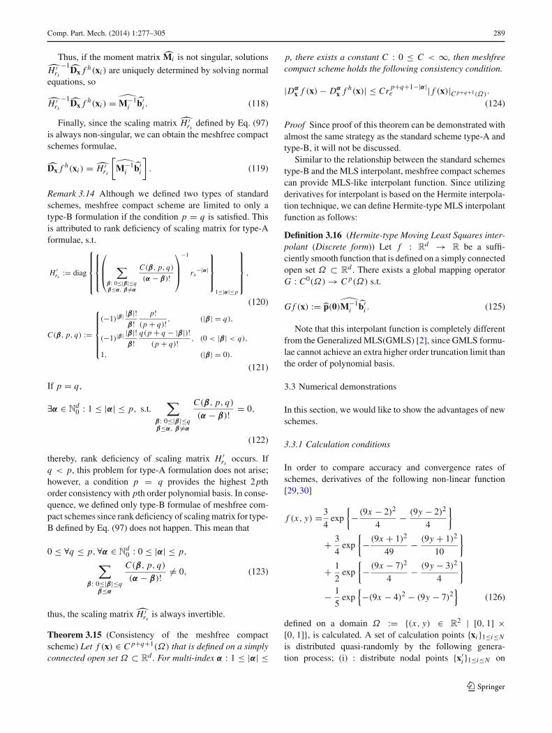
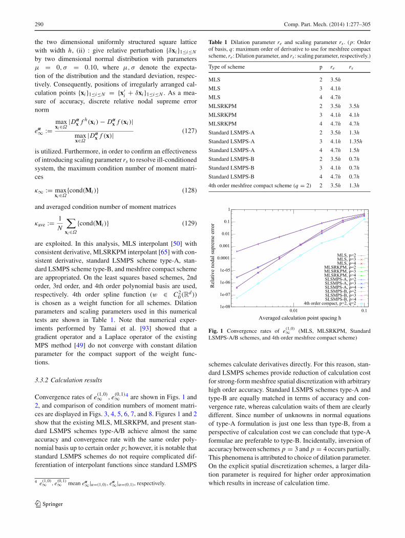
Convergence rates of e(1,0)∞ , e(0,1)∞ 4 are shown in Figs. 1 and2, and comparison of condition numbers of moment matri-ces are displayed in Figs. 3, 4, 5, 6, 7, and 8. Figures 1 and 2show that the existing MLS, MLSRKPM, and present stan-dard LSMPS schemes type-A/B achieve almost the sameaccuracy and convergence rate with the same order poly-nomial basis up to certain order p; however, it is notable thatstandard LSMPS schemes do not require complicated dif-ferentiation of interpolant functions since standard LSMPS

4 e(1,0)∞ , e(0,1)∞ mean eα∞|α=(1,0), eα∞|α=(0,1), respectively.

Table 1 Dilation parameter re and scaling parameter rs . (p: Orderof basis, q: maximum order of derivative to use for meshfree compactscheme, re: Dilation parameter, and rs : scaling parameter, respectively.)

Type of scheme p re rs

MLS 2 3.5h

MLS 3 4.1h

MLS 4 4.7h

MLSRKPM 2 3.5h 3.5h

MLSRKPM 3 4.1h 4.1h

MLSRKPM 4 4.7h 4.7h

Standard LSMPS-A 2 3.5h 1.3h



Standard LSMPS-B 2 3.5h 0.7h



4th order meshfree compact scheme (q = 2) 2 3.5h 1.3h

Fig. 1 Convergence rates of e(1,0)∞ (MLS, MLSRKPM, StandardLSMPS-A/B schemes, and 4th order meshfree compact scheme)

schemes calculate derivatives directly. For this reason, stan-dard LSMPS schemes provide reduction of calculation costfor strong-form meshfree spatial discretization with arbitraryhigh order accuracy. Standard LSMPS schemes type-A andtype-B are equally matched in terms of accuracy and con-vergence rate, whereas calculation waits of them are clearlydifferent. Since number of unknowns in normal equationsof type-A formulation is just one less than type-B, from aperspective of calculation cost we can conclude that type-Aformulae are preferable to type-B. Incidentally, inversion ofaccuracy between schemes p = 3 and p = 4 occurs partially.This phenomena is attributed to choice of dilation parameter.On the explicit spatial discretization schemes, a larger dila-tion parameter is required for higher order approximationwhich results in increase of calculation time.

123

Comp. Part. Mech. (2014) 1:277–305 291

Fig. 2 Convergence rates of e(0,1)∞ (MLS, MLSRKPM, StandardLSMPS-A/B schemes, and 4th order meshfree compact scheme)

Fig. 3 Averaged condition number of moment matrices (MLS,MLSRKPM, LSMPS) (p = 2)



Fig. 6 Maximum condition number of moment matrices (MLS,MLSRKPM, LSMPS) (p = 2)


123

292 Comp. Part. Mech. (2014) 1:277–305


Worthy of special mention is excellent accuracy of mesh-free compact scheme. Drawing a comparison between 2nd-order explicit schemes and 4th-order meshfree compactscheme with the same dilation parameter and the same orderbasis demonstrates higher accuracy of the compact scheme,and it beyonds comparison. Moreover, comparing between4th-order explicit schemes and 4th-order meshfree compactscheme shows the advantage of meshfree compact schemefrom the standpoint of accuracy. Note that if 4th-order poly-nomial basis is utilized for least squares approximation,meshfree compact scheme can achieve up to 8th order con-sistency for the first derivatives. Although meshfree compactschemes require several times iterative procedure, they cancontribute astonishingly higher accuracy and higher orderconvergence rate than existing explicit meshfree spatial dis-cretization schemes.

Figures 3, 4, 5, 6, 7, and 8 demonstrate that the effects ofintroducing scaling parameter rs for the basis of the weightedleast squares method are significant. Condition numbers ofMLS moment matrix are not bounded, in other words, smallercalculation point spacing makes larger condition number ofmoment matrix.5 This is extremely dangerous case in numer-ical calculation. On the other hand, maximum conditionnumbers of MLSRK moment matrces and LSMPS momentmatrices are uniformly bounded; however, condition num-bers of MLSRK moment matrixces are certainly larger thanLSMPS’s. As discussed in Remark 3.2, introducing scalingparameter rs instead of dilation parameter re is a slight changefrom the idea of MLSRK basis; however, it makes an enor-mous difference for the condition number. Lower conditionnumber provided by the present technique yields avoidance

5 Order of MLS moment matrix’s condition number is evaluated asO(r−2p

e ), see [92]

of ill-conditioned problem which results in enhancement ofstability and accuracy in practical numerical calculations.6

4 Time integration scheme and boundary conditions

4.1 The rotational pressure-correction projection method

The classical projection scheme of Chorin [22] based on theHelmholtz decomposition theorem and its derivations arecommonly utilized for numerical analyses of incompress-ible flow. Consider the incompressible flow governed by theNavier–Stokes equations and the mass conservation

∇ · u = 0, (130)

DuDt

= − 1

ρ∇ P + ν∇2u + f, (131)

where u, ρ, ν, P, f denotes velocity vector, density, kine-matic viscosity, pressure, and body force, respectively. Thereare a lot of derivations of projection scheme. For instance,assume that u be a sufficiently smooth function, the pressure-correction schemes can be written into the following gener-alized form [33]:

1st Step :

βs u −s−1∑

j=0

β j uk− j

Δt= ν∇2u − 1

ρ∇ P� + f(tk+1), (132)

with boundary condition

u∣∣∣Γ

= 0. (133)

2nd Step :

βs

Δt

(uk+1 − u

)= − 1

ρ∇φk+1, (134)

with boundary conditions

∇ · uk+1 = 0, (135)

uk+1 · n∣∣∣Γ

= 0, (136)

6 In practical numerical analyses, there exist not only round-off errorsof floating-point arithmetics but also numerical errors. In this numer-ical convergence study, exact functional values { f (xi )}1≤i≤n are sub-stituted into the right hand side vectors {b(xi )}1≤i≤n , then they containonly round-off errors; however, in practical simulation of continuum,the right hand side vectors must have numerical errors (e.g. numeri-cal errors of pressure, velocity.). Ill-conditioned problems will enlargethese errors; therefore, keeping linear systems to be well-conditionedwith lower condition number is crucially important.

123

Comp. Part. Mech. (2014) 1:277–305 293

∂φk+1

∂n

∣∣∣∣Γ

= 0, (137)

where Γ denotes the boundary of a domain, and modifiedpressure φ is defined as follows:

φk+1 = Pk+1 − P� + χμ∇ · u, (138)

P� =

⎧⎪⎪⎪⎪⎨

⎪⎪⎪⎪⎩

0, (r = 0),

Pk, (r = 1),

2Pk − Pk−1, (r = 2),

... (r ≥ 3).

(139)

Although sth order backward difference formulae thatapproximate Du/Dt are applied in the above equations,other consistent time discretization schemes are perfectlyacceptable.7 χ is a user-defined coefficient that equal to0 or 1. The choice χ = 0 yields the standard pressure-correction projection schemes, whereas χ = 1 gives therotational pressure-correction schemes. An important differ-ence between the standard pressure-correction schemes andthe rotational forms appear in the Neumann boundary condi-tion for pressure Poisson equations. The former enforce thehomogeneous Neumann boundary condition, s.t.

⎧⎪⎪⎪⎪⎪⎪⎪⎪⎪⎪⎨

⎪⎪⎪⎪⎪⎪⎪⎪⎪⎪⎩

∂ Pk+1

∂n

∣∣∣∣Γ

= 0, (r = 0),

∂ Pk+1

∂n

∣∣∣∣Γ

− ∂ Pk

∂n

∣∣∣∣Γ

= 0

�⇒ ∂ Pk+1

∂n

∣∣∣∣Γ

= ∂ Pk

∂n

∣∣∣∣Γ

= · · · = ∂ P0

∂n

∣∣∣∣Γ

, (r = 1),

... (r ≥ 2),

(140)

this non-physical inconsistent Neumann boundary condi-tions enforced on the pressure introduces the numericalboundary layer which limits the accuracy of time integra-tion schemes [33,83]. The later, the rotational schemes, how-ever, enforce the non-homogeneous Neumann boundary con-dition, s.t.

∂ Pk+1

∂n

∣∣∣∣Γ

=[−μ∇ × ∇ × uk+1 + ρf(tk+1)

]· n

∣∣∣∣Γ

, (141)

which, unlike Eq. (140), is a consistent pressure bound-ary condition derived from a velocity boundary conditionu · n|Γ . This is the origin of the name of “rotational” projec-

7 For instance, in our experience, The well-known Crank–Nicolsonscheme provides excellent results in terms of calculation cost andnumerical accuracy.

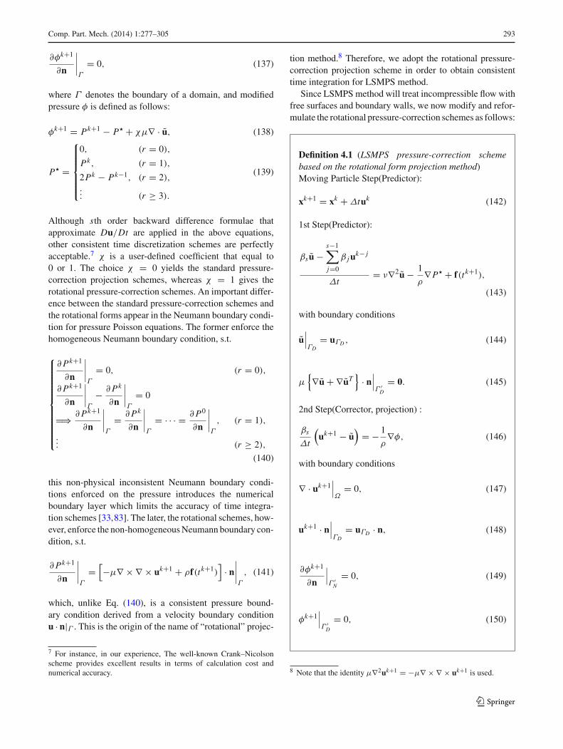
tion method.8 Therefore, we adopt the rotational pressure-correction projection scheme in order to obtain consistenttime integration for LSMPS method.

Since LSMPS method will treat incompressible flow withfree surfaces and boundary walls, we now modify and refor-mulate the rotational pressure-correction schemes as follows:

Definition 4.1 (LSMPS pressure-correction schemebased on the rotational form projection method)Moving Particle Step(Predictor):

xk+1 = xk + Δtuk (142)

1st Step(Predictor):

βs u −s−1∑

j=0

β j uk− j

Δt= ν∇2u − 1

ρ∇ P� + f(tk+1),

(143)


u∣∣∣ΓD

= uΓD , (144)

μ{∇u + ∇uT

}· n∣∣∣Γ ′

D

= 0. (145)

2nd Step(Corrector, projection) :

βs

Δt

(uk+1 − u

)= − 1

ρ∇φ, (146)


∇ · uk+1∣∣∣Ω

= 0, (147)

uk+1 · n∣∣∣ΓD

= uΓD · n, (148)

∂φk+1

∂n

∣∣∣Γ ′

N

= 0, (149)

φk+1∣∣∣Γ ′

D

= 0, (150)

8 Note that the identity μ∇2uk+1 = −μ∇ × ∇ × uk+1 is used.

123

294 Comp. Part. Mech. (2014) 1:277–305

where modified pressure φ is defined as follows:

φk+1 = Pk+1 − P� + μ∇ · u. (151)

Moving Particle Step(Corrector, if needed) :

xk+1 = xk + Δt

2

(uk+1 + uk

)(152)

In Definition 4.1, ΓD, Γ ′D, Γ ′

N denotes Dirichlet bound-ary (boundary wall) on the velocity, Dirichlet boundary (freesurface) on the pressure, and Neumann boundary (bound-ary wal) on the pressure, respectively. Taking divergence ofEq. (146) and utilizing divergence free condition of the veloc-ity ∇ · uk+1 = 0 yield modified pressure Poisson equations,s.t.

∇2φk+1 = βsρ

Δt∇ · u, (153)


φk+1∣∣∣Γ ′

D

= 0, (154)

∂φk+1

∂n

∣∣∣Γ ′

N

= 0. (155)

It should be noticed that if Dirichlet boundary condition onthe pressure Pk+1|Γ ′

D= 0 were enforced, Dirichlet boundary

condition on the modified pressure would be φk+1|Γ ′D

= μ∇·u. On the free surfaces, incompressible condition ∇ · u = 0must be satisfied, then Dirichlet boundary condition on themodified pressure would be φk+1|Γ ′

D= 0. Note that solving

modified pressure Poisson equation (153) is equivalent tocalculating consistent pressure Poisson equations s.t.

∇2 Pk+1 = ∇2 P� − μ∇2(∇ · u) + βsρ

Δt∇ · u, (156)

with consistent non-homogeneous Neumann boundary con-dition. One can observe from Eq. (153) and (156) that sourceterm of consistent Poisson equation is simplified by the intro-duction of the rotational forms.

Note that time discretization schemes applied on the mov-ing particle steps and the velocity evolution steps can bereplaced any other higher order time discretization schemes.

4.2 Generalized Neumann boundary conditionsenforcement

In numerical calculations, treatment of boundary conditionsplays a role as important as consistency and stability of dis-cretization schemes. In order to consummate LSMPS method

as a numerical method for solving partial differential equa-tions, we have to consider both Dirichlet and Neumannboundary conditions on the velocity or the pressure.

Since LSMPS method is based on the strong-form formu-lations, Dirichlet boundary conditions can be easily treatedby substitutiing of boundary values. On the other hand, Neu-mann boundary condition enforcing is relatively difficult.This seems to be commonality in the strong-form numeri-cal methods. For instance, in the FDM, utilizing higher orderspatial discretization schemes yields more complicated for-mulations of “one-sided finite difference schemes” to enforceNeumann boundary conditions. This problem is a remarkabletendency in two or three dimensional analysis which resultsin difficulty of programming code implementation and main-tenance.

In the existing particle method with semi-implicit algo-rithm for incompressible fluid such as projection SPH method[23], incompressible SPH method [85], and MPS method[49], “dummy particle” approach for boundary walls is usu-ally applied, and homogeneous pressure Neumann boundarycondition is implemented with modification procedures ofcoefficient matrix for the discretized Laplace operator of thepressure Poisson equations; however, they are inconsistentas long as their discrete Laplace operator schemes and thehomogeneous pressure boundary condition enforcement areinconsistent.

In order to construct a generalized procedure to enforceconsistent Neumann boundary conditions, we define a newconstrained scheme based on the weighted least squaresmethod.

Recall that we introduced variable transformations toavoid ill-conditioned linear system derived from the leastsquares procedures s.t.

Dαx f h(x) −→ r |α|

s

α! Dαx f h(x)

to formulate Standard LSMPS schemes type-A/B, andassume that outer normal unit vector n is uniquely definedon the boundary of the domain Γ and Neumann boundarycondition of sufficiently smooth function f is given by

∂ f (x)

∂n= gN (x). (157)

This Neumann boundary condition can be rewritten equiva-lently as

∂ f (x)

∂n= gN (x) (158)

⇐⇒∑

|α|=1

nα Dαx f (x) = gN (x) (159)

123

Comp. Part. Mech. (2014) 1:277–305 295

⇐⇒∑

|α|=1

nα

{r |α|

s

α! Dαx f (x)

}= rs gN (x) (160)

⇐⇒pTN (x)

[H−1

rsDx f (x)

]= rs gN (x) (161)

⇐⇒pNT (x)

[Hrs

−1Dx f (x)]

= rs gN (x) (162)

where

pN (x) :=⎛

⎝n∣∣∣x, 0, · · · , 0︸︷︷︸

σ times

⎞

⎠ , (163)

pN (x) :=⎛

⎝0, n∣∣∣x, 0, · · · , 0︸︷︷︸

σ times

⎞

⎠ , (164)

σ :=(

p + d

d

)− (d + 1), (165)

and rs > 0 is the scaling parameter. Equations (161) and(162) can be viewed as one of the equations that constructsnormal equations derived from the weighted least squaresmethod since unknowns are common. Thus, if we define a

discrete functional associated with R p+1i j ,

R p+1

i j , Eqs. (161)and (162), s.t.

JN (H−1rs

Dx f h(xi )) (166)

:=∑

j∈Λi

w

(x j − xi

re

)(R p+1

i j

)2

+ wN (xi , re)

[pT

N

∣∣∣xi

[H−1

rsDx f h(xi )

]− rs gN (x)

]2

,

(167)

JN (Hrs

−1Dx f h(xi ))

:=∑

j∈Λi

w

(x j − xi

re

)(R p+1

i j

)2

+ wN (xi , re)

[pN

T∣∣∣xi

[Hrs

−1Dx f h(xi )]

− rs gN (x)

]2

,

(168)

they provide normal equations. The choice of weight wN

(xi , re) for Neumann boundary condition enforcement isarbitrary. In this study, we utilize the following:

wN (xi , re) := maxx∈Rd

w(x, re). (169)

Note that this choice requires non-singular weight func-tion usage. Then, if moment matrices of normal equationsprovided by minimizing Eqs. (166) and (168) are non-

singular, we can obtain constraint LSMPS schemes type-A/B to enforce arbitrary Neumann boundary condition asfollows:

Definition 4.2 (Constraint LSMPS scheme, Type-A)Let f : R

d → R be a sufficiently smooth function ona simply connected open set Ω ⊂ R

d and assume thatouter normal unit vector n ∈ R

d is uniquely defined onthe boundary of domain ΓN , Γ ′

N , and Neumann bound-ary condition ∂ f (x)/∂n|ΓN ,Γ ′

N= gN (x) is given. Con-

straint LSMPS schemes Type-A are defined as follows:

Dx f h(xi ) := Hrs

[[Mi + Ni ]

−1 {bi + ci }]

(170)

where

Dx := {Dα

x | 1 ≤ |α| ≤ p}, (171)

Hrs := diag

{{rs

−|α|α!}

1≤|α|≤p

}, (172)

Mi :=∑

j∈Λi

[w

(‖x j − xi‖re

)

p(

x j − xi

rs

)pT(

x j − xi

rs

)],

(173)

Ni := wN

(‖xi‖re

)pN (xi ) pT

N (xi ) , (174)

bi :=∑

j∈Λi

[w

(‖x j − xi‖re

)(175)

p(

x j − xi

rs

){ f (x j ) − f (xi )}

], (176)

ci := wN

(‖xi‖re

)pN (xi ) rs gN (xi ), (177)

p (x) := {xα | 1 ≤ |α| ≤ p

}, (178)

pN (x) :=⎛

⎝n∣∣∣x, 0, · · · , 0︸︷︷︸

σ times

⎞

⎠ , (179)

σ :=(

p + d

d

)− (d + 1), (180)

wN

(‖xi‖re

)= max

x∈Rdw(x, re) (181)

Λi :={

j∣∣∣ 0 ≤ ‖x j − xi‖ < re

}(182)




123

296 Comp. Part. Mech. (2014) 1:277–305

Definition 4.3 (Constraint LSMPS scheme, Type-B)Let f : R

d → R be a sufficiently smooth function ona simply connected open set Ω ⊆ R

d and assume thatouter normal unit vector n ∈ R

d is uniquely defined onthe boundary of domain ΓN , Γ ′

N , and Neumann bound-ary condition ∂ f (x)/∂n|ΓN ,Γ ′

N= gN (x) is given. Con-

straint LSMPS schemes Type-B are defined as follows:

Dx f h(xi ) := Hrs

[[Mi + Ni

]−1 {bi + ci

}](183)

where

Dx := {Dα

x | 0 ≤ |α| ≤ p}, (184)

Hrs := diag

{{rs

−|α|α!}

0≤|α|≤p

}, (185)

Mi :=∑

j∈Λi

[w

(‖x j − xi‖re

)(186)

p(

x j − xi

rs

)pT(

x j − xi

rs

)], (187)

Ni := wN

(‖xi‖re

)pN (xi ) pN

T (xi ) , (188)

bi :=∑

j∈Λi

[w

(‖x j − xi‖re

)p(

x j − xi

rs

)f (x j )

],

(189)

ci := wN

(‖xi‖re

)pN (xi ) rs gN (xi ), (190)

p (x) := {xα | 0 ≤ |α| ≤ p

}, (191)

pN (x) :=⎛

⎝0, n∣∣∣x, 0, · · · , 0︸︷︷︸

σ times

⎞

⎠ , (192)

σ :=(

p + d

d

)− (d + 1), (193)

wN

(‖xi‖re

)= max

x∈Rdw(x, re) (194)

Λi :={

j∣∣∣ 0 ≤ ‖x j − xi‖ < re

}(195)




Remark 4.4 Since moment matrices of linear systems arechanged with additional terms Ni , Ni , the conditions ofmoment matrix invertibility are relaxed. In other words, adsc-ititious outer normal vector n for the moment matrix acts as

the position of the additive virtual calculation point. More-over, it moves “the center of gravity of particles”, minifiesthe condition number of moment matrix, and provides animprovement of accuracy near the domain boundary.

4.3 Surface boundary particle detection algorithm

In order to run analyses of fluid flow with free surfaces withLagrangian description, dynamic algorithm to detect surfaceboundary particles is required. In the MPS method [49], avery simple algorithm is utilized. Let ni be a parameter called“particle number density”9 of particle xi defined by

ni :=∑

j �=i

w(x j − xi , re), (196)

and n∗i , n0 denotes a particle number density pre-solving

pressure Poisson equations and a reference particle numberdensity, respectively. The MPS surface boundary detectionalgorithm is that, if a particle xi satisfies

n∗i < βn0, (197)

then it will be judged as a particle on the surface boundary;otherwise, it will be treated as a particle in interior of domain.β is a user-defined tuning parameter, and is usually chosento be in the range of β = 0.80−0.97. Very similar algorithmis introduced for incompressible SPH method [85] that thecondition is

ρ∗i < βρ0, (198)

where ρ denotes the density that is defined by

ρi :=∑

j

mw(x j − xi , re). (199)

These algorithm are very simple, however, erroneous deci-sion of surface boundary particle, which yields unphysicaloscillation of pressure fields, often occurs. Various proposalto solve this problem have been sought, for instance, alter-native or additive conditions such as usage of the center ofgravity of the particles [32], gradient of the particle num-ber density [40], and divergence of particle position [52] areintroduced; however, incorrect judgements remains.

Boundary detection algorithm based on the particular geo-metrical conditions are also proposed, for example, “Arcmethod” for the MLSPH method [24,25] provides excel-lent results. Koh et al. also utilize Arc method for the MPSmethod [46]; however, it has a deal killer that extension of thealgorithm for three dimensional surface boundary detection

9 It should be called “weight function density” for more accuratedescription.

123

Comp. Part. Mech. (2014) 1:277–305 297

must be severely complex. Actually, Haque and Dilts con-structed the methodology of three dimensional arc method[35]; however, it is exceedingly complicated and requireshigh computational cost.

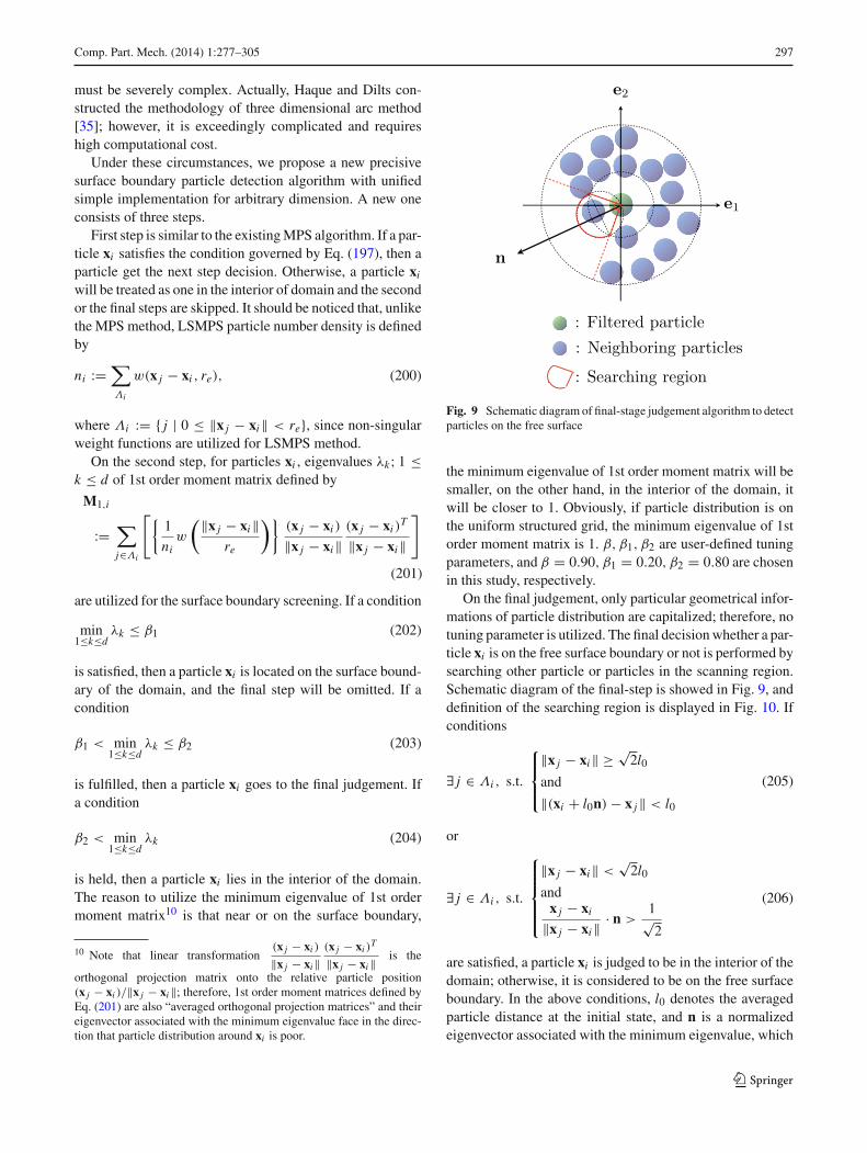
Under these circumstances, we propose a new precisivesurface boundary particle detection algorithm with unifiedsimple implementation for arbitrary dimension. A new oneconsists of three steps.

First step is similar to the existing MPS algorithm. If a par-ticle xi satisfies the condition governed by Eq. (197), then aparticle get the next step decision. Otherwise, a particle xi

will be treated as one in the interior of domain and the secondor the final steps are skipped. It should be noticed that, unlikethe MPS method, LSMPS particle number density is definedby

ni :=∑

Λi

w(x j − xi , re), (200)

where Λi := { j | 0 ≤ ‖x j − xi‖ < re}, since non-singularweight functions are utilized for LSMPS method.

On the second step, for particles xi , eigenvalues λk; 1 ≤k ≤ d of 1st order moment matrix defined by

M1,i

:=∑

j∈Λi

[{1

niw

(‖x j − xi‖re

)}(x j − xi )

‖x j − xi‖(x j − xi )

T

‖x j − xi‖

]

(201)

are utilized for the surface boundary screening. If a condition

min1≤k≤d

λk ≤ β1 (202)

is satisfied, then a particle xi is located on the surface bound-ary of the domain, and the final step will be omitted. If acondition

β1 < min1≤k≤d

λk ≤ β2 (203)

is fulfilled, then a particle xi goes to the final judgement. Ifa condition

β2 < min1≤k≤d

λk (204)

is held, then a particle xi lies in the interior of the domain.The reason to utilize the minimum eigenvalue of 1st ordermoment matrix10 is that near or on the surface boundary,

10 Note that linear transformation(x j − xi )

‖x j − xi ‖(x j − xi )

T

‖x j − xi ‖ is the

orthogonal projection matrix onto the relative particle position(x j − xi )/‖x j − xi ‖; therefore, 1st order moment matrices defined byEq. (201) are also “averaged orthogonal projection matrices” and theireigenvector associated with the minimum eigenvalue face in the direc-tion that particle distribution around xi is poor.

e1

e2

n

: Filtered particle

: Neighboring particles

: Searching region

Fig. 9 Schematic diagram of final-stage judgement algorithm to detectparticles on the free surface

the minimum eigenvalue of 1st order moment matrix will besmaller, on the other hand, in the interior of the domain, itwill be closer to 1. Obviously, if particle distribution is onthe uniform structured grid, the minimum eigenvalue of 1storder moment matrix is 1. β, β1, β2 are user-defined tuningparameters, and β = 0.90, β1 = 0.20, β2 = 0.80 are chosenin this study, respectively.

On the final judgement, only particular geometrical infor-mations of particle distribution are capitalized; therefore, notuning parameter is utilized. The final decision whether a par-ticle xi is on the free surface boundary or not is performed bysearching other particle or particles in the scanning region.Schematic diagram of the final-step is showed in Fig. 9, anddefinition of the searching region is displayed in Fig. 10. Ifconditions

∃ j ∈ Λi , s.t.

⎧⎪⎨

⎪⎩

‖x j − xi‖ ≥ √2l0

and

‖(xi + l0n) − x j‖ < l0

(205)

or

∃ j ∈ Λi , s.t.

⎧⎪⎪⎪⎨

⎪⎪⎪⎩

‖x j − xi‖ <√

2l0and

x j − xi

‖x j − xi‖ · n >1√2

(206)

are satisfied, a particle xi is judged to be in the interior of thedomain; otherwise, it is considered to be on the free surfaceboundary. In the above conditions, l0 denotes the averagedparticle distance at the initial state, and n is a normalizedeigenvector associated with the minimum eigenvalue, which

123

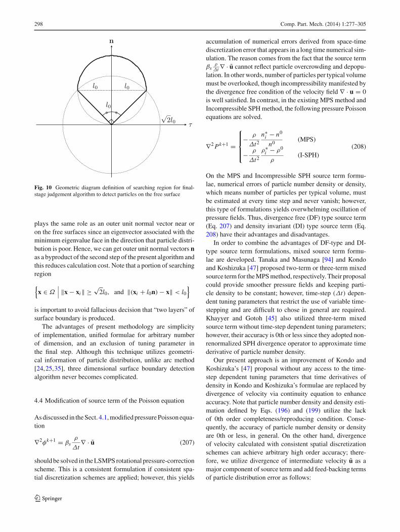
298 Comp. Part. Mech. (2014) 1:277–305

n

τ

√2l0

l0 l0

l0

Fig. 10 Geometric diagram definition of searching region for final-stage judgement algorithm to detect particles on the free surface

plays the same role as an outer unit normal vector near oron the free surfaces since an eigenvector associated with theminimum eigenvalue face in the direction that particle distri-bution is poor. Hence, we can get outer unit normal vectors nas a byproduct of the second step of the present algorithm andthis reduces calculation cost. Note that a portion of searchingregion

{x ∈ Ω

∣∣∣ ‖x − xi‖ ≥ √2l0, and ‖(xi + l0n) − x‖ < l0

}

is important to avoid fallacious decision that “two layers” ofsurface boundary is produced.

The advantages of present methodology are simplicityof implementation, unified formulae for arbitrary numberof dimension, and an exclusion of tuning parameter inthe final step. Although this technique utilizes geometri-cal information of particle distribution, unlike arc method[24,25,35], three dimensional surface boundary detectionalgorithm never becomes complicated.

4.4 Modification of source term of the Poisson equation

As discussed in the Sect. 4.1, modified pressure Poisson equa-tion

∇2φk+1 = βsρ

Δt∇ · u (207)

should be solved in the LSMPS rotational pressure-correctionscheme. This is a consistent formulation if consistent spa-tial discretization schemes are applied; however, this yields

accumulation of numerical errors derived from space-timediscretization error that appears in a long time numerical sim-ulation. The reason comes from the fact that the source termβs

ρΔt ∇ · u cannot reflect particle overcrowding and depopu-

lation. In other words, number of particles per typical volumemust be overlooked, though incompressibility manifested bythe divergence free condition of the velocity field ∇ · u = 0is well satisfied. In contrast, in the existing MPS method andIncompressible SPH method, the following pressure Poissonequations are solved.

∇2 Pk+1 =

⎧⎪⎪⎨

⎪⎪⎩

− ρ

Δt2

n∗i − n0

n0 (MPS)

− ρ

Δt2

ρ∗i − ρ0

ρ(I-SPH)

(208)

On the MPS and Incompressible SPH source term formu-lae, numerical errors of particle number density or density,which means number of particles per typical volume, mustbe estimated at every time step and never vanish; however,this type of formulations yields overwhelming oscillation ofpressure fields. Thus, divergence free (DF) type source term(Eq. 207) and density invariant (DI) type source term (Eq.208) have their advantages and disadvantages.

In order to combine the advantages of DF-type and DI-type source term formulations, mixed source term formu-lae are developed. Tanaka and Masunaga [94] and Kondoand Koshizuka [47] proposed two-term or three-term mixedsource term for the MPS method, respectively. Their proposalcould provide smoother pressure fields and keeping parti-cle density to be constant; however, time-step (Δt) depen-dent tuning parameters that restrict the use of variable time-stepping and are difficult to chose in general are required.Khayyer and Gotoh [45] also utilized three-term mixedsource term without time-step dependent tuning parameters;however, their accuracy is 0th or less since they adopted non-renormalized SPH divergence operator to approximate timederivative of particle number density.

Our present approach is an improvement of Kondo andKoshizuka’s [47] proposal without any access to the time-step dependent tuning parameters that time derivatives ofdensity in Kondo and Koshizuka’s formulae are replaced bydivergence of velocity via continuity equation to enhanceaccuracy. Note that particle number density and density esti-mation defined by Eqs. (196) and (199) utilize the lackof 0th order completeness/reproducing condition. Conse-quently, the accuracy of particle number density or densityare 0th or less, in general. On the other hand, divergenceof velocity calculated with consistent spatial discretizationschemes can achieve arbitrary high order accuracy; there-fore, we utilize divergence of intermediate velocity u as amajor component of source term and add feed-backing termsof particle distribution error as follows:

123

Comp. Part. Mech. (2014) 1:277–305 299

Definition 4.5 (LSMPS modified Pressure Poissonequations and boundary conditions)

∇2φk+1 = βsρ

Δt(∇ · u)

+ ρ

Δt

∣∣∣∣∣nk − n0

n0

∣∣∣∣∣ (∇ · uk)

+ ρ

Δt

∣∣∇ · uk∣∣(

nk − n0

n0

)(209)


φk+1∣∣∣Γ ′

D

= 0 (210)

∂φk+1

∂n

∣∣∣Γ ′

N

= 0 (211)

The second term of Eq. (208) is a error correction term

of divergence free condition, and |(nk − n0)/n0| is a non-dimensional semi-positive coefficient. The third term is aerror adjustment term of particle number density invariant,and |∇ · uk | is a semi-positive coefficient chosen to haveappropriate dimension. Note that successive refinement pro-cedures of time-space subdivisions make ∇ · uk to be zero;therefore, error correction terms must vanish when incom-pressibility of the fluid is numerically satisfied. n0 is the mod-ified reference of particle number density defined by

n0 = NFilled cell

NTotal cell

∫

Rd

w(x, re)dx (212)

In the above equation, the coefficient NFilled cell/NTotal cell isa remediation factor for the lack of 0th to approximate parti-cle number density defined by Eq. (196). Consider a uniformstructured local background cell with spacing l0. Schematicdiagram is shown in Fig.11. NTotal cell is the total numberof local background cells, which must be well-adopted forthe dilation parameter re and number of dimension d.11

NFilled cell is the number of local background cells occupiedby a particle or particles. NFilled cell count increment is differ-ent for each particle types. Fluid particles in the interior ofthe domain are counted with weight 1, and fluid particles onthe free surface boundary or wall boundary are enumerated

11 For example, if re = 3.1 ≈ 3 and d = 2 are chosen, NTotal cell =(2×re)

2 ≈ 62 = 36. If re = 3.1 ≈ 3 and d = 3 are chosen, NTotal cell =(2 × re)

3 ≈ 63 = 216. Determination of NTotal cell must be flexible forthe choice of dilation parameter.

: Fluid particle in interior domain

: Fluid particle on free surfaces: Fluid and wall particle on wall

xi xi

: Fully filled cell: Half filled cell: Void cell

re

e1

e2

l0

l0

Fig. 11 Schematic diagram of particle number density modificationwith utilizing temporary local background cell

with weight 1/2. If two or more particles exist in a cell, themaximum count of this cell is limited to be 1. This simpleprocedures should be perfumed not to all but particles thatincludes boundary particle in their own support of weightfunction. This present modification must enhance accuracyof particle number density approximation dramatically nearor on the boundaries.

5 Numerical example

In order to demonstrate the advantage of the present LSMPSmethod comparing with the existing MPS method, twodimensional dam-collapse (dam-break) problem is chosen asa benchmark problem. Since dam-collapse problem includesfree surfaces (Dirichlet boundary on the pressure and Neu-mann boundary on the velocity), boundary wall (Dirichletboundary on the velocity and Neumann boundary on the pres-

0.8[m]

0.2[m]

0.4[m]

0 .5[m]

Gravity 9.8[m/s2]

Fig. 12 Schematic diagram of initial state of fluid and fixed boundarywall for the two dimensional dam collapse problem

123

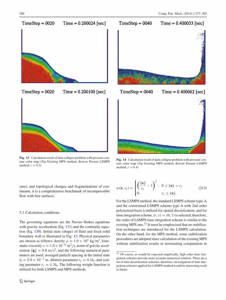
300 Comp. Part. Mech. (2014) 1:277–305

Fig. 13 Calculation result of dam collapse problem with pressure con-tour color map (Top Existing MPS method, Bottom Present LSMPSmethod, t = 0.2)

sure), and topological changes and fragmentations of con-tinuum, it is a comprehensive benchmark of incompressibleflow with free surfaces.

5.1 Calculation conditions

The governing equations are the Navier–Stokes equationswith gravity acceleration (Eq. 131) and the continuity equa-tion (Eq. 130). Initial state (shape) of fluid and fixed solidboundary wall is illustrated in Fig. 12. Physical parametersare chosen as follows: density ρ = 1.0 × 103 kg/m3, kine-matic viscosity ν = 1.0×10−6 m2/s, norm of gravity accel-eration ‖g‖ = 9.8 m/s2, and the following numerical para-meters are used: averaged particle spacing at the initial statel0 = 5.0 × 10−3 m, dilation parameter re = 4.1l0, and scal-ing parameter rs = 1.3l0. The following weight function isutilized for both LSMPS and MPS methods.


w(x, re) =

⎧⎪⎨

⎪⎩

(‖x‖re

− 1

)2

, 0 ≤ ‖x‖ < re

0, re ≤ ‖x‖.(213)

For the LSMPS method, the standard LSMPS scheme type-Aand the constrained LSMPS scheme type-A with 2nd orderpolynomial basis is utilized for spatial discretization, and fortime integration scheme, (r, s) = (0, 1) is selected; therefore,the order of LSMPS time integration scheme is similar to theexisting MPS one.12 It must be emphasized that no stabiliza-tion techniques are introduced for the LSMPS calculation.On the other hand, for the MPS method, some stabilizationprocedures are adopted since calculation of the existing MPSwithout stabilization results in terminating computation in

12 Of course, as would be expected empirically, high order time inte-gration schemes provide more accurate numerical solution. There are alot of time discretization schemes, therefore, investigation of time inte-gration schemes applied for LSMPS method would be interesting workin future.

123

Comp. Part. Mech. (2014) 1:277–305 301


early times of numerical simulation. In particular, stabiliza-tion method such as collision model [47], gradient operatormodification [48], and pressure modification that negativepressure is corrected to be zero, are introduced only for theMPS method.


5.2 Calculation results

Snapshots of calculation results (t = 0.2, . . . , 1.2) with con-tour plot of pressure fields are shown in Figs. 13, 14, 15, 16,17, and 18, and the time evolutions of pressure observedon a sampling points A and B are displayed in Figs. 19

123

302 Comp. Part. Mech. (2014) 1:277–305


and 20. Figures 13, 14, 15, 16, 17, and 18 shows that theexisting MPS solutions suffered from unphysical pressureoscillation. In contrast, LSMPS solutions provide smootherpressure field without numerical oscillation. One can observefrom Figs. 13, 14, 15, 16, 17, and 18 that clarity of freesurface boundary is demonstrably different. Smoother pres-sure field contributes to stable motions of particles, whichresults in unambiguity of deformable fluid interfaces. More-over, Figs. 19 and 20 demonstrate that LSMPS solutions pro-duce smooth pressure evolution in both space and time. Now


Fig. 19 Time evolution of pressure on a sampling point A

123

Comp. Part. Mech. (2014) 1:277–305 303

Fig. 20 Time evolution of pressure on a sampling point B

we can gain release from problem such as serious numericalpressure oscillation.

The major differences between the MPS method and theLSMPS method in this analysis are the order of spatial dis-cretization schemes, pressure Neumann boundary condition,pressure source term of Poisson equation, and surface bound-ary particle detection algorithm. We have to mention that thismore accurate and stable calculation can be obtained onlyby an introduction of the combination of new proposals. Inother words, implementation of one improvement would befrustrated by a variety of factors. Since LSMPS formulaepresented in this study can achieve arbitrary high order accu-racy, more accurate solution can be widely expected from anapplication of higher order schemes.

6 Conclusion

In this paper, a new consistent meshfree-Lagrangian approachfor incompressible flow with free surfaces, named LeastSquares Moving Particle Semi-implicit (LSMPS) method isdeveloped. This methodology includes arbitrary high orderconsistent meshfree spatial discretization schemes, time inte-gration schemes with consistent boundary conditions, andgeneralized treatment of Neumann boundary conditions.Application of new proposals to benchmark problem demon-strates conspicuous enhancement of stability and accuracy.Excellent accuracy of new meshfree compact schemes gener-alized for arbitrary dimension and high order of consistencyis worthy of special mention. They are applicable for not onlyincompressible flows but also any targets governed by partialdifferential equations in meshfree framework; therefore, thisnew meshfree method can be utilized as one of the powerfultools to obtain high order accurate numerical solutions.

References

1. Aluru N (2000) A point collocation method based on reproducingKernel approximations. Int J Numer Methods Eng 47(6):1083–1121

2. Atluri S, Cho J, Kim HG (1999) Analysis of thin beams, using themeshless local Petrov–Galerkin method, with generalized movingleast squares interpolations. Comput Mech 24(5):334–347

3. Atluri S, Zhu T (1998) A new meshless local Petrov–Galerkin(mlpg) approach in computational mechanics. Comput Mech22(2):117–127

4. Atluri S, Zhu T (2000) New concepts in meshless methods. Int JNumer Methods Eng 47(1–3):537–556

5. Atluri S, Zhu TL (2000) The meshless local Petrov–Galerkin(mlpg) approach for solving problems in elasto-statics. ComputMech 25(2–3):169–179

6. Atluri SN, Kim HG, Cho JY (1999) A critical assessmentof the truly meshless local Petrov–Galerkin (mlpg), and localboundary integral equation (lbie) methods. Comput Mech 24(5):348–372

7. Babuska I, Melenk JM (1995) The partition of unity finite elementmethod. Tech. rep, DTIC Document

8. Babuska I, Melenk JM (1996) The partition of unity method. IntJ Numer Methods Eng 40(1):727–758

9. Babuška I, Zhang Z (1998) The partition of unity method forthe elastically supported beam. Comput Methods Appl Mech Eng152(1):1–18

10. Balsara DS, Shu CW (2000) Monotonicity preserving weightedessentially non-oscillatory schemes with increasingly high orderof accuracy. J Comput Phys 160(2):405–452

11. Belytschko T, Gu L, Lu Y (1994) Fracture and crack growthby element free Galerkin methods. Modell Simul Mater Sci Eng2(3A):519

12. Belytschko T, Krongauz Y, Dolbow J, Gerlach C (1998) On thecompleteness of meshfree particle methods. Int J Numer MethodsEng 43(5):785–819

13. Belytschko T, Lu Y, Gu L (1995) Crack propagation by element-free Galerkin methods. Eng Fract Mech 51(2):295–315

14. Belytschko T, Lu Y, Gu L, Tabbara M (1995) Element-freeGalerkin methods for static and dynamic fracture. Int J SolidsStruct 32(17):2547–2570

15. Belytschko T, Lu YY, Gu L (1994) Element-free Galerkin meth-ods. Int J Numer Methods Eng 37(2):229–256

16. Bonet J, Kulasegaram S (2000) Correction and stabilization ofsmooth particle hydrodynamics methods with applications inmetal forming simulations. Int J Numer Methods Eng 47(6):1189–1214

17. Chakravarthy SR (1970) Some new approaches to grid generation,discretization, and solution methods for cfd. In: Proceedings of4th international symposium computational fluid dynamics 14,pp. 403–420

18. Chen J, Beraun J (2000) A generalized smoothed particle hydro-dynamics method for nonlinear dynamic problems. ComputMethods Appl Mech Eng 190(1):225–239

19. Chen J, Beraun J, Carney T (1999) A corrective smoothed particlemethod for boundary value problems in heat conduction. Int JNumer Methods Eng 46(2):231–252

20. Chen J, Beraun J, Jih C (1999) Completeness of correctivesmoothed particle method for linear elastodynamics. ComputMech 24(4):273–285

21. Chen JS, Pan C, Wu CT, Liu WK (1996) Reproducing Kernel par-ticle methods for large deformation analysis of non-linear struc-tures. Comput Methods Appl Mech Eng 139(1):195–227

22. Chorin AJ (1968) Numerical solution of the Navier–Stokes equa-tions. Math Comput 22(104):745–762

123

304 Comp. Part. Mech. (2014) 1:277–305

23. Cummins SJ, Rudman M (1999) An sph projection method. JComput Phys 152(2):584–607

24. Dilts GA (1999) Moving-least-squares-particle hydrodynamics.Consistency and stability. Int J Numer Methods Eng 44(8):1115–1155

25. Dilts GA (2000) Moving least-squares particle hydrodynam-ics ii: conservation and boundaries. Int J Numer Methods Eng48(10):1503–1524

26. Donea J, Giuliani S, Halleux J (1982) An arbitrary Lagrangian–Eulerian finite element method for transient dynamic fluid–structure interactions. Comput Methods Appl Mech Eng33(1):689–723

27. Duarte CA, Oden JT (1996) An h-p adaptive method using clouds.Comput Methods Appl Mech Eng 139(1):237–262

28. Duarte CA, Oden JT (1996) Hp clouds-an hp meshless method.Numer Methods Partial Differ Equ 12(6):673–706

29. Franke R (1979) A critical comparison of some methods for inter-polation of scattered data. Tech. rep, DTIC Document

30. Franke R (1982) Scattered data interpolation: tests of some meth-ods. Math Comput 38(157):181–200

31. Gingold RA, Monaghan JJ (1977) Smoothed particlehydrodynamics-theory and application to non-spherical stars.Mon Noti R Astron Soc 181:375–389

32. Gotoh H, Khayyer A, Hori C (2009) New assessment criterion offree surface for stabilizing pressure field in particle method. JpnSoc Civil Eng Series B2 (Coastal Eng) 2:21–25

33. Guermond J, Minev P, Shen J (2006) An overview of projectionmethods for incompressible flows. Comput Methods Appl MechEng 195(44):6011–6045

34. Han W, Meng X (2001) Error analysis of the reproducing Kernelparticle method. Comput Methods Appl Mech Eng 190(46):6157–6181

35. Haque A, Dilts GA (2007) Three-dimensional boundary detectionfor particle methods. J Comput Phys 226(2):1710–1730

36. Hirt C, Amsden AA, Cook J (1974) An arbitrary lagrangian-eulerian computing method for all flow speeds. J Comput Phys14(3):227–253

37. Hughes TJ (2012) The finite element method: linear sta-tic and dynamic finite element analysis. Dover Publications,Mineola

38. Idelsohn SR, Oñate E, Pin FD (2004) The particle finite ele-ment method: a powerful tool to solve incompressible flows withfree-surfaces and breaking waves. Int J Numer Methods Eng61(7):964–989

39. Iribe T, Nakaza E (2010) A precise calculation method of thegradient operator in numerical computation with the mps. J JpnSoc Civil Eng B 66(1):46–50

40. Itori S, Iribe T, Nakaza E. An improvement of dirichlet boundaryconditions in numerical simulations using mps method. Japan SocCivil Eng B2 (Coastal Eng)

41. Johnson GR, Beissel SR (1996) Normalized smoothing func-tions for sph impact computations. Int J Numer Methods Eng39(16):2725–2741

42. Khayyer A, Gotoh H (2008) Development of cmps method foraccurate water-surface tracking in breaking waves. Coast Eng J50(02):179–207

43. Khayyer A, Gotoh H (2009) Modified moving particle semi-implicit methods for the prediction of 2d wave impact pressure.Coast Eng 56(4):419–440

44. Khayyer A, Gotoh H (2010) A higher order Laplacian model forenhancement and stabilization of pressure calculation by the mpsmethod. Appl Ocean Res 32(1):124–131

45. Khayyer A, Gotoh H (2011) Enhancement of stability and accu-racy of the moving particle semi-implicit method. J Comput Phys230(8):3093–3118

46. Koh C, Gao M, Luo C (2012) A new particle method for simu-lation of incompressible free surface flow problems. Int J NumerMethods Eng 89(12):1582–1604

47. Kondo M, Koshizuka S (2011) Improvement of stability in mov-ing particle semi-implicit method. Int J Numer Methods Fluids65(6):638–654

48. Koshizuka S, Nobe A, Oka Y (1998) Numerical analysis of break-ing waves using the moving particle semi-implicit method. Int JNumer Methods Fluids 26(7):751–769

49. Koshizuka S, Oka Y (1996) Moving-particle semi-implicitmethod for fragmentation of incompressible fluid. Nucl Sci Eng123(3):421–434

50. Lancaster P, Salkauskas K (1981) Surfaces generated by movingleast squares methods. Math Comput 37(155):141–158

51. Lax PD, Richtmyer RD (1956) Survey of the stability of linearfinite difference equations. Commun Pure Appl Math 9(2):267–293

52. Lee ES, Moulinec C, Xu R, Violeau D, Laurence D, StansbyP (2008) Comparisons of weakly compressible and truly incom-pressible algorithms for the sph mesh free particle method. J Com-put Phys 227(18):8417–8436

53. Lele SK (1992) Compact finite difference schemes with spectral-like resolution. J Comput Phys 103(1):16–42

54. Li S, Liu WK (1999) Reproducing Kernel hierarchical partitionof unity, part iformulation and theory. Int J Numer Methods Eng45(3):251–288

55. Li S, Liu WK (2004) Meshfree particle methods, vol 11. Springer,Dordrecht

56. Li S, Lu H, Han W, Liu WK, Simkins DC (2004) ReproducingKernel element method part ii: globally conforming im/cn hier-archies. Comput Methods Appl Mech Eng 193(12):953–987

57. Liszka T (1984) An interpolation method for an irregular net ofnodes. Int J Numer Methods Eng 20(9):1599–1612

58. Liszka T, Duarte C, Tworzydlo W (1996) hp-meshless cloudmethod. Comput Methods Appl Mech Eng 139(1):263–288

59. Liszka T, Orkisz J (1980) The finite difference method at arbitraryirregular grids and its application in applied mechanics. ComputStruct 11(1):83–95

60. Liu GGR, Liu M (2003) Smoothed particle hydrodynamics: ameshfree particle method. World Scientific, Singapore

61. Liu WK, Chen Y, Uras RA, Chang CT (1996) Generalized multi-ple scale reproducing Kernel particle methods. Comput MethodsAppl Mech Eng 139(1):91–157

62. Liu WK, Han W, Lu H, Li S, Cao J (2004) Reproducing kernelelement method. Part 1: theoretical formulation. Comput MethodsAppl Mech Eng 193(12):933–951

63. Liu WK, Jun S, Li S, Adee J, Belytschko T (1995) Reproduc-ing Kernel particle methods for structural dynamics. Int J NumerMethods Eng 38(10):1655–1679

64. Liu WK, Jun S, Zhang YF (1995) Reproducing Kernel particlemethods. Int J Numer Methods Fluids 20(8–9):1081–1106

65. Liu WK, Li S, Belytschko T (1997) Moving least-square repro-ducing Kernel methods (i) methodology and convergence. Com-put Methods Appl Mech Eng 143(1):113–154

66. Lu H, Li S, Simkins DC Jr, Kam Liu W, Cao J (2004) Reproducingkernel element method part iii: generalized enrichment and appli-cations. Comput Methods Appl Mech Eng 193(12):989–1011

67. Lu Y, Belytschko T, Gu L (1994) A new implementation of theelement free Galerkin method. Comput Methods Appl Mech Eng113(3):397–414

68. Lucy LB (1977) A numerical approach to the testing of the fissionhypothesis. Astron J 82:1013–1024

69. Melenk JM, Babuška I (1996) The partition of unity finite elementmethod: basic theory and applications. Comput Methods ApplMech Eng 139(1):289–314

123

Comp. Part. Mech. (2014) 1:277–305 305

70. Monaghan JJ (1988) An introduction to sph. Comput Phys Com-mun 48(1):89–96

71. Monaghan JJ (1992) Smoothed particle hydrodynamics. Ann RevAstron Astrophys 30:543–574

72. Monaghan JJ (2005) Smoothed particle hydrodynamics. Rep ProgPhys 68(8):1703

73. Nayroles B, Touzot G, Villon P (1992) Generalizing the finite ele-ment method: diffuse approximation and diffuse elements. Com-put Mech 10(5):307–318

74. Oden J, Duarte C, Zienkiewicz O (1998) A new cloud-basedhp finite element method. Comput Methods Appl Mech Eng153(1):117–126

75. Oñate E, Idelsohn S (1998) A mesh-free finite point method foradvective-diffusive transport and fluid flow problems. ComputMech 21(4–5):283–292

76. Oñate E, Idelsohn S, Zienkiewicz O, Taylor R (1996) A finite pointmethod in computational mechanics. applications to convectivetransport and fluid flow. Int J Numer Methods Eng 39(22):3839–3866

77. Oñate E, Idelsohn S, Zienkiewicz O, Taylor R, Sacco C (1996)A stabilized finite point method for analysis of fluid mechanicsproblems. Comput Methods Appl Mech Eng 139(1):315–346

78. Oñate E, Idelsohn SR, Celigueta MA, Rossi R (2008) Advancesin the particle finite element method for the analysis of fluid-multibody interaction and bed erosion in free surface flows. Com-put Methods Appl Mech Eng 197(19):1777–1800

79. Oñate E, Idelsohn SR, Del Pin F, Aubry R (2004) The parti-cle finite element methodan overview. Int J Comput Methods1(02):267–307

80. Oñate E, Perazzo F, Miquel J (2001) A finite point method forelasticity problems. Comput Struct 79(22):2151–2163

81. Quinlan NJ, Basa M, Lastiwka M (2006) Truncation error in mesh-free particle methods. Int J Numer Methods Eng 66(13):2064–2085

82. Randles P, Libersky L (1996) Smoothed particle hydrodynamics:some recent improvements and applications. Comput MethodsAppl Mech Eng 139(1):375–408

83. Rannacher R (1992) On Chorin’s projection method for the incom-pressible Navier–Stokes equations. Springer, Berlin

84. Rudin W (1976) Principles of mathematical analysis (Interna-tional Series in Pure & Applied Mathematics). McGraw-Hill, NewYork

85. Shao S, Lo EY (2003) Incompressible sph method for simulatingNewtonian and non-Newtonian flows with a free surface. AdvWater Resour 26(7):787–800

86. Simkins DC Jr, Li S, Lu H (2004) Kam Liu, W.: Reproducing ker-nel element method. part iv: globally compatible cn (n 1) triangu-lar hierarchy. Comput Methods Appl Mech Eng 193(12):1013–1034

87. Smith G (1985) Numerical solution of partial differential equa-tions: finite difference methods. Oxford applied mathematics andcomputing science series. Clarendon Press, Oxford

88. Stone MH (1937) Applications of the theory of boolean rings togeneral topology. Trans Am Math Soc 41(3):375–481

89. Stone MH (1948) The generalized weierstrass approximation the-orem. Math Mag 21(5):237–254

90. Strikwerda J (2007) Finite difference schemes and partial differ-ential equations. SIAM, Philadelphia

91. Suzuki Y (2007) Ph.D. thesis, The University of Tokyo, Japan92. Tamai T (2014) Development of least squares moving particle

semi-implicit method. Master’s Thesis, The University of Tokyo,Japan

93. Tamai, T, Shibata K, Koshizuka S (2013) Development of thehigher-order mps method using the taylor expansion. Trans JpnSoc Comput Eng Sci 2013 (20130003)

94. Tanaka M, Masunaga T (2010) Stabilization and smoothing ofpressure in mps method by quasi-compressibility. J Comput Phys229(11):4279–4290

95. Tiwari S, Kuhnert J (2003) Finite pointset method based on theprojection method for simulations of the incompressible navier-stokes equations. Meshfree methods for partial differential equa-tions. Springer, Berlin, pp 373–387

96. Tiwari S, Kuhnert J (2005) A numerical scheme for solvingincompressible and low mach number flows by the finite pointsetmethod. Meshfree methods for partial differential equations II.Springer, Berlin, pp 191–206

97. Tiwari S, Kuhnert J (2007) Modeling of two-phase flows withsurface tension by finite pointset method (fpm). J Comput ApplMath 203(2):376–386

98. Versteeg H, Malalasekera W (2007) An introduction to computa-tional fluid dynamics: the finite volume method. Pearson Educa-tion Limited, Singapore

99. Zhang G, Batra R (2004) Modified smoothed particle hydrody-namics method and its application to transient problems. ComputMech 34(2):137–146

100. Zhang G, Batra R (2009) Symmetric smoothed particle hydro-dynamics (ssph) method and its application to elastic problems.Comput Mech 43(3):321–340

101. Zienkiewicz OC, Taylor RL (1977) The finite element method,vol 3. McGraw-Hill, London

123

least squares moving particle semi-implicit method · least squares moving particle semi-implicit...

Documents