International MacroeconomicsLecture 2

Laura Sunder-Plassmann

University of Copenhagen

Fall 2015

International business cycles

I What do business cycles around the world look like?

I A �rst look at the data - what we will ask our theories toexplain later on

I Reference: SGU 1, Cooley 11, also almost all the theoreticalpapers we discuss later (Baxter Crucini 1995, BKK 1992,Heathcote Perri 2000)

De�ning business cycles

I We are not trying to study secular phenomena (growth,development), but cyclical �uctuations

I Decompose time series yt into trend y st and cyclicalcomponent y ct

yt = y st + y ct

I There are di�erent ways to do this. Common:

I Log-linear detrendingI Log-quadratic detrendingI Hodrick Prescott (HP) �lteringI First di�erencing

Example 1: Log-linear detrending

I Let yt denote the natural logarithm of a time series Yt and t atime trend

yt = lnYt = a+ bt + εt

cycle: y ct = εt

trend: y st = a+ bt

I The parameters a and b can be estimated via OLS

I Di�erent trend for each country/ variable usually

Example 2: Log-quadratic detrending

I Let yt denote the natural logarithm of a time series Yt and t atime trend

yt = lnYt = a+ bt + ct2 + εt

cycle: y ct = εt

trend: y st = a+ bt + ct2

I The parameters a, b and c can be estimated via OLS

I 3 cycles. Picks up hyperin�ation in the late 1980s anddefault/currency crisis in early 2000s

I Very volatile (standard deviation 10.7%) and persistent(correlation yt,, yt−1 0.85) cycle

Business cycle facts around the world

I Panel data set: all countries with ≥ 30 years of consecutivedata, 1960-2010

I Frequency: Annual, for availability reasons

I Data source: World Bank WDI, publicly available

I Alternatives: OECD Statistics, IMF International FinancialStatistics (IFS) and World Economic Outlook (WEO),Eurostat, national sources

I Variables:

I yt = lnYt natural log GDP, constant prices, per capitaI ct log private consumption, constant prices, per capitaI it log investment, constant prices, per capitaI xt log exports, constant prices, per capitaI mt log imports, constant prices, per capitaI gt log government consumption, constant prices, per capita

Business cycle facts around the world

I For each country, compute (i) standard deviations, (ii),contemporaneous correlations and (iii) serial correlations ofeach variable

I Then compute population-weighted average of each statisticacross countries

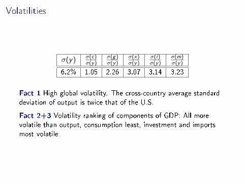
Volatilities

σ(y) σ(c)σ(y)

σ(g)σ(y)

σ(x)σ(y)

σ(i)σ(y)

σ(m)σ(y)

6.2% 1.05 2.26 3.07 3.14 3.23

Fact 1 High global volatility. The cross-country average standarddeviation of output is twice that of the U.S.

Fact 2+3 Volatility ranking of components of GDP: All morevolatile than output, consumption least, investment and importsmost volatile

Cyclicality (correlations with output)

ρ(c , y) ρ(i , y) ρ(gy , y) ρ(x , y) ρ(m, y) ρ(tby , y)

0.69 0.66 -0.02 0.19 0.24 -0.15

Fact 4 Components of GDP are positively correlated with output

Fact 5 Trade balance to output ratio is negatively correlated withoutput

Fact 6 Government consumption to output ratio is acyclical

Persistence

ρ(yt , yt−1) 0.71

ρ(ct , ct−1) 0.66

ρ(gt , gt−1) 0.76

ρ(it , it−1) 0.56

ρ(xt , xt−1) 0.68

ρ(mt ,mt−1) 0.61

Fact 7 Output and its components are all positively seriallycorrelated

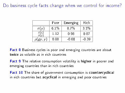
Do business cycle facts change when we control for income?

Poor Emerging Rich

σ(y) 6.1% 8.7% 3.3%σ(c)σ(y) 1.12 0.98 0.87

ρ(gy , y) 0.08 -0.08 -0.39

Fact 8 Business cycles in poor and emerging countries are abouttwice as volatile as in rich countries

Fact 9 The relative consumption volatility is higher in poorer andemerging countries than in rich countries

Fact 10 The share of government consumption is countercyclicalin rich countries but acyclical in emerging and poor countries

The Hodrick Prescott (1997) �lterAre the results robust to alternative methods of detrending?

I The Hodrick Prescott (1997) �lter: Given a time series yt , fort=1,2,...,T, pick y ct and y st to

min{y c

t ,yst }∞t=0

{T∑t=1

(y ct )2 + λ

T−1∑t=2

[(y st+1 − y st )− (y st − y st−1)

]2}subject to y ct + y st = yt

where λ is a parameter

I When λ→∞, change in the growth rate of ytbecomein�nitely costly, and the HP trend component converges to alog-linear trend

The size of λ matters

I Quarterly data: 1600

I Annual data: 100. Some authors suggest 6.25

I Example: Argentina

λ 100 6.25

σ(y) 6.3% 3.6%

The size of λ matters

International business cycle co-movement

I So far we've talked about national business cycle facts onaverage across the world

I What about the links between countries? Are economies inrecessions at the same time, for example?

I Many papers that document this, for example BKK in Cooley(see reading list)

I OECD countriesI 1970.1-1991.2I OECD QNA, employment from MEI

International business cycle co-movement

Fact 11 Business cycles are highly synchronizedFact 12 Consumption is less correlated across countries thanoutputFact 13 Investment and hours are positively correlated

Conclusion

I We took a �rst look at the data

I Described key empirical reuglarities of international businesscycles

I If you choose to remember only 1 thing from today: The tradebalance is countercyclical

I If 2: Business cycles are highly synchronized across countries

I We will discover additional relevant empirical facts as we startreading papers