lecture 1: introduction and motivation - xuhappy.github.io · motivation of the course • do you...

Lecture 1: Introduction and Motivation

Huanle Xu

Big Data Analytics

1

Motivation

• Do you want to work in these companies?

2

Motivation of the Course

• Do you want to understand what is big data?What are the main characteristics of big data?

• Do you want to understand the infrastructureand techniques of big data analytics?

• Do you want to know the research challengesin the area of big data learning and mining?

3

Course Objective

1. To understand the current key issues on big dataand the associated business/scientific dataapplications;

2. To teach the fundamental techniques andframeworks in achieving big data analytics withscalability and streaming capability

3. To understand basic optimization methods towardssolving big data related problems

4. Able to apply software tools for big dataanalytics

4

Course Description• Course Homepage: https://xuhappy.github.io/courses/BigData/• This course aims at teaching students the state-of-the-art big data

analytics, including techniques, software, applications, and perspectives with massive data.

• The class will cover, but not be limited to, the following topics:– cloud computing, big data processing frameworks, distributed file systems

such as Google File System, Hadoop Distributed File System, CloudStore, and map-reduce technology;

– machine learning technology, SVM models, Deep Neural Networks– Data Mining Methods, Clustering, Dimension Reduction, Recommendation systems– optimization methods, convex optimization, online learning

5

Textbook for Reference• Mining of Massive Datasets• Anand Rajaraman

– web and technology entrepreneur– co-founder of Cambrian Ventures and

Kosmix– co-founder of Junglee Corp (acquired

by Amazon for a retail platform)• Jeff Ullman

– The Stanford W. Ascherman Professorof Computer Science (Emeritus)

– Interests in database theory, databaseintegration, data mining, andeducation using the informationinfrastructure.

6

Textbook

• Amazon– http://www.amazon.com/Mining-Massive-

Datasets-Anand-Rajaraman/dp/1107015359

• PDF of the book for online viewing– http://infolab.stanford.edu/~ullman/mmds.html

7

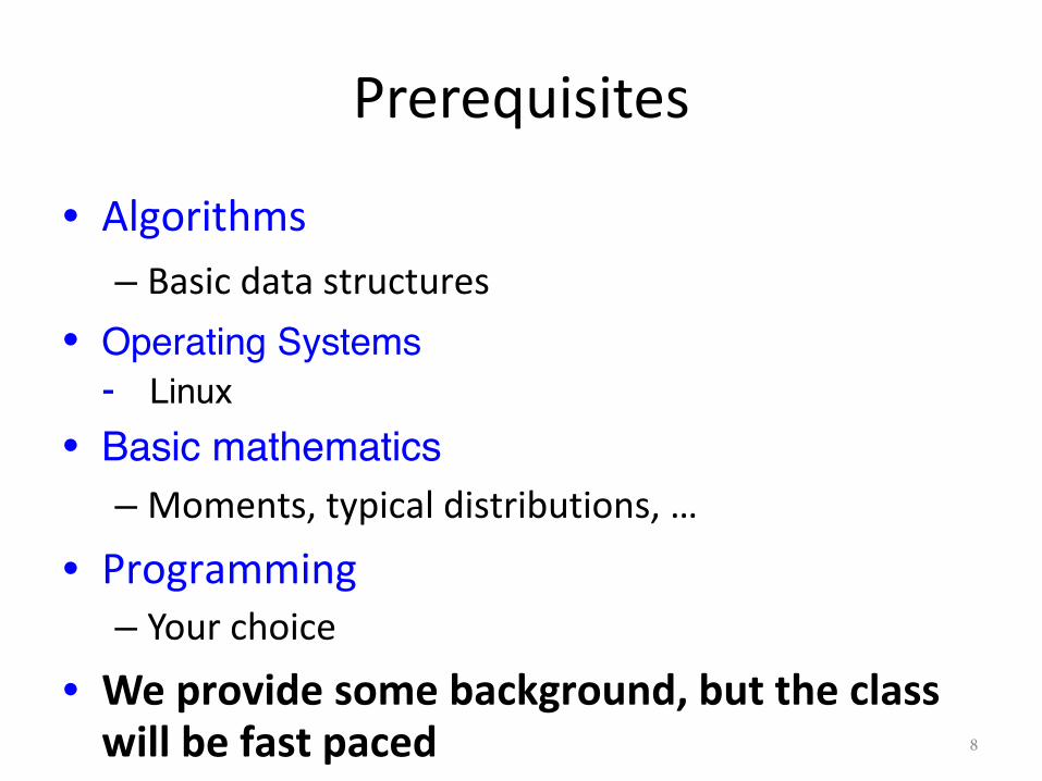
http://www.amazon.com/Mining-Massive-Datasets-Anand-Rajaraman/dp/1107015359

http://infolab.stanford.edu/%7Eullman/mmds.html

Prerequisites

• Algorithms– Basic data structures

• Operating Systems- Linux

• Basic mathematics – Moments, typical distributions, …

• Programming– Your choice

• We provide some background, but the class will be fast paced 8

What Will We Learn?

• We will learn to analyze different types of data:– Data is high dimensional– Data is a graph– Data is infinite/never-ending– Data is labeled

• We will learn to use different models ofcomputation:– MapReduce– Streams and online algorithms– Single machine in-memory

9

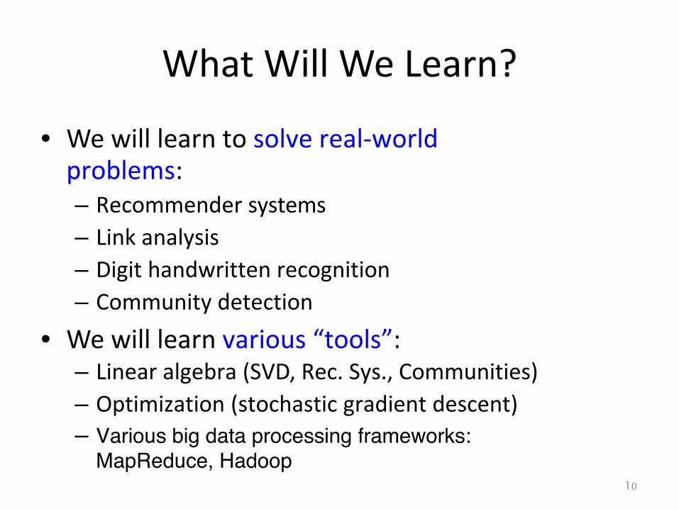
What Will We Learn?

• We will learn to solve real-worldproblems:– Recommender systems– Link analysis– Digit handwritten recognition– Community detection

• We will learn various “tools”:– Linear algebra (SVD, Rec. Sys., Communities)– Optimization (stochastic gradient descent)– Various big data processing frameworks:

MapReduce, Hadoop10

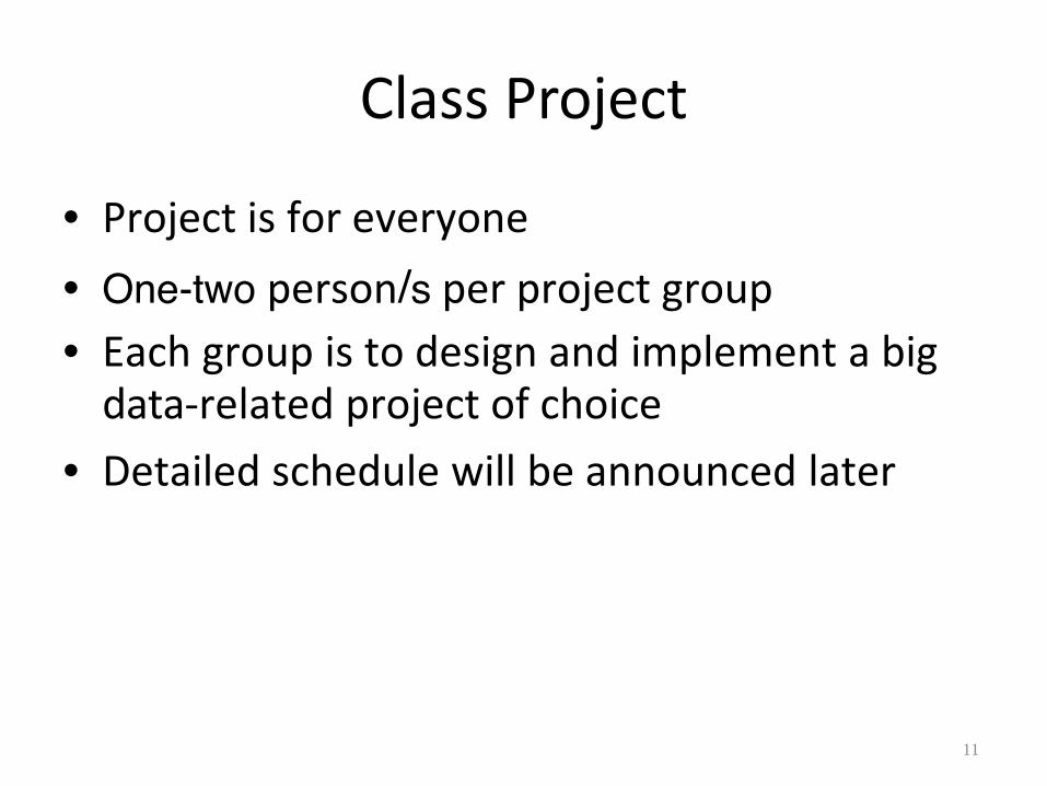
Class Project

• Project is for everyone• One-two person/s per project group• Each group is to design and implement a big

data-related project of choice• Detailed schedule will be announced later

11

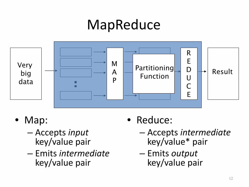
MapReduce

• Map:– Accepts input

key/value pair– Emits intermediate

key/value pair

Very bigdata

ResultMAP

REDUCE

PartitioningFunction

• Reduce:– Accepts intermediate

key/value* pair– Emits output

key/value pair12

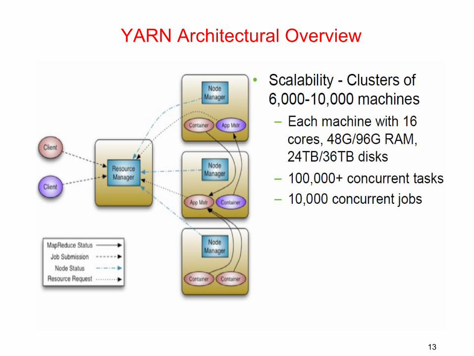
13

YARN Architectural Overview

Mining Data Stream

• Stream Management is important when theinput rate is controlled externally:– Google queries– Twitter or Facebook status updates

• We can think of the data as infinite and non-stationary (the distribution changes over time)

14

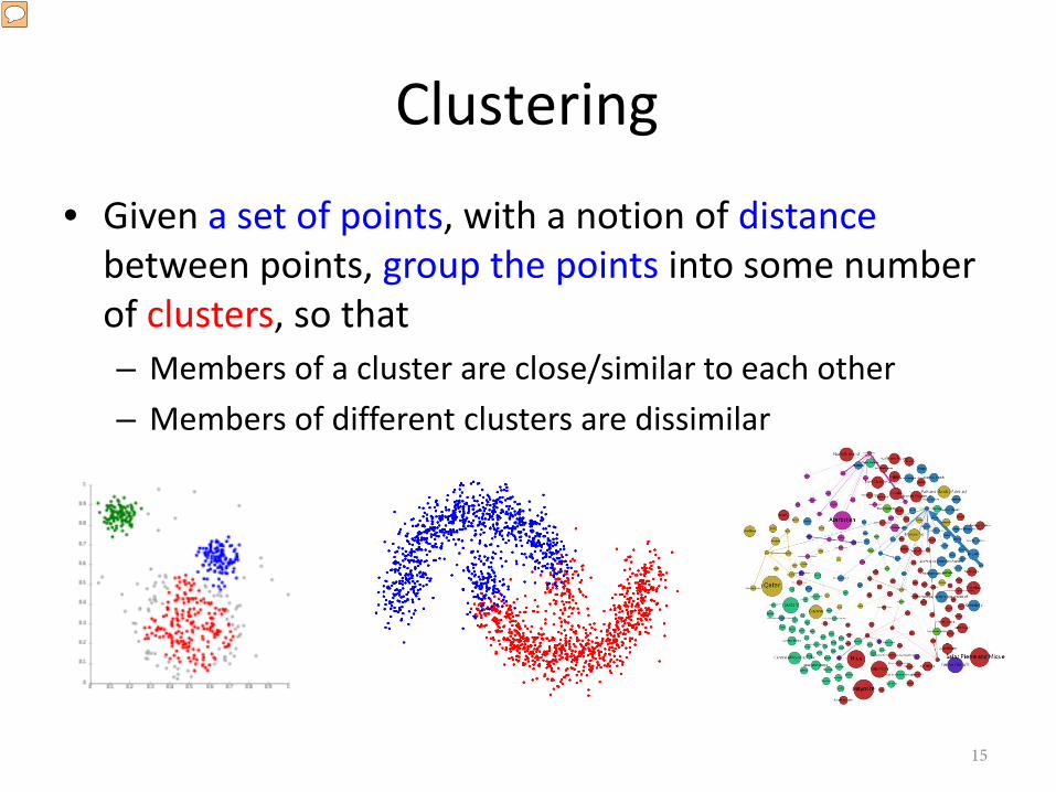
Clustering

• Given a set of points, with a notion of distancebetween points, group the points into some numberof clusters, so that– Members of a cluster are close/similar to each other– Members of different clusters are dissimilar

15

Presenter

Presentation Notes

To understand the structure of the data

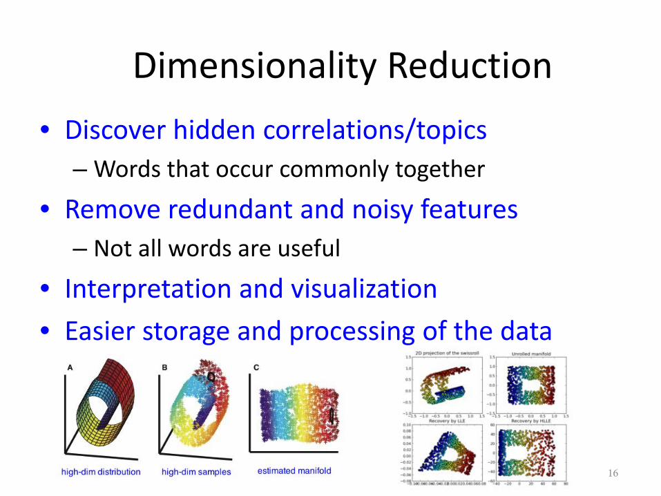
Dimensionality Reduction• Discover hidden correlations/topics

– Words that occur commonly together

• Remove redundant and noisy features– Not all words are useful

• Interpretation and visualization• Easier storage and processing of the data

16

Recommender System

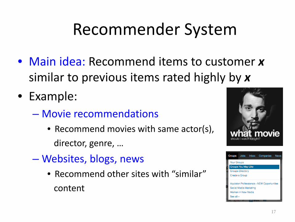
• Main idea: Recommend items to customer xsimilar to previous items rated highly by x

• Example:– Movie recommendations

• Recommend movies with same actor(s),director, genre, …

– Websites, blogs, news• Recommend other sites with “similar”

content

17

Link Analysis

• Computing importance of nodes in a graph

18

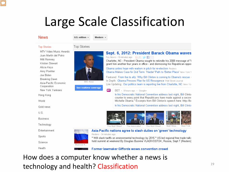
Large Scale Classification

How does a computer know whether a news is technology and health? Classification 19

Presenter

Presentation Notes

News change every second, volume is large

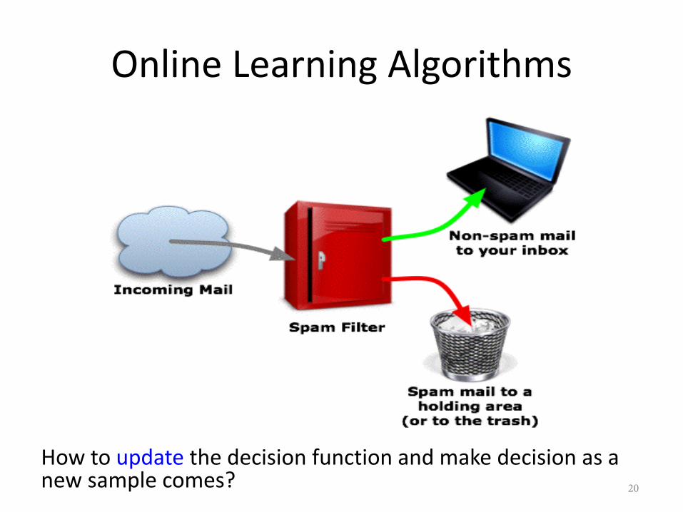
Online Learning Algorithms

How to update the decision function and make decision as a new sample comes? 20

Introduction to Big Data

21

Definition of Big Data

• Big data is a collection of data sets so largeand complex that it becomes difficult toprocess using on-hand database managementtools or traditional data processingapplications.

From wiki

22

http://en.wikipedia.org/wiki/Big_data

Evolution of Big Data

• Birth: 1880 US census• Adolescence: Big Science• Modern Era: Big Business

23

Birth: 1880 US census

24

The First Big Data Challenge

• 1880 census• 50 million people• Age, gender (sex),

occupation, educationlevel, no. of insanepeople in household

25

Presenter

Presentation Notes

Took over seven years to manually tabulate and report on the data

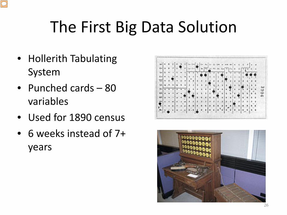
The First Big Data Solution

• Hollerith TabulatingSystem

• Punched cards – 80variables

• Used for 1890 census• 6 weeks instead of 7+

years

26

Presenter

Presentation Notes

A mechanical device called the Hollerith Tabulating system, which worked with punch cards that could hold about 80 variables. The HT system revolutionized the value of census data, making it actionable and increasing its value an untold amount. Analysis took six weeks instead of seven years. It allowed the government to act on information in a reasonable amount of time. The ability to analyze the 1890 census led to an improved understanding of the populace, which the government could use to shape economic and social policies ranging from taxation to education to military conscription.

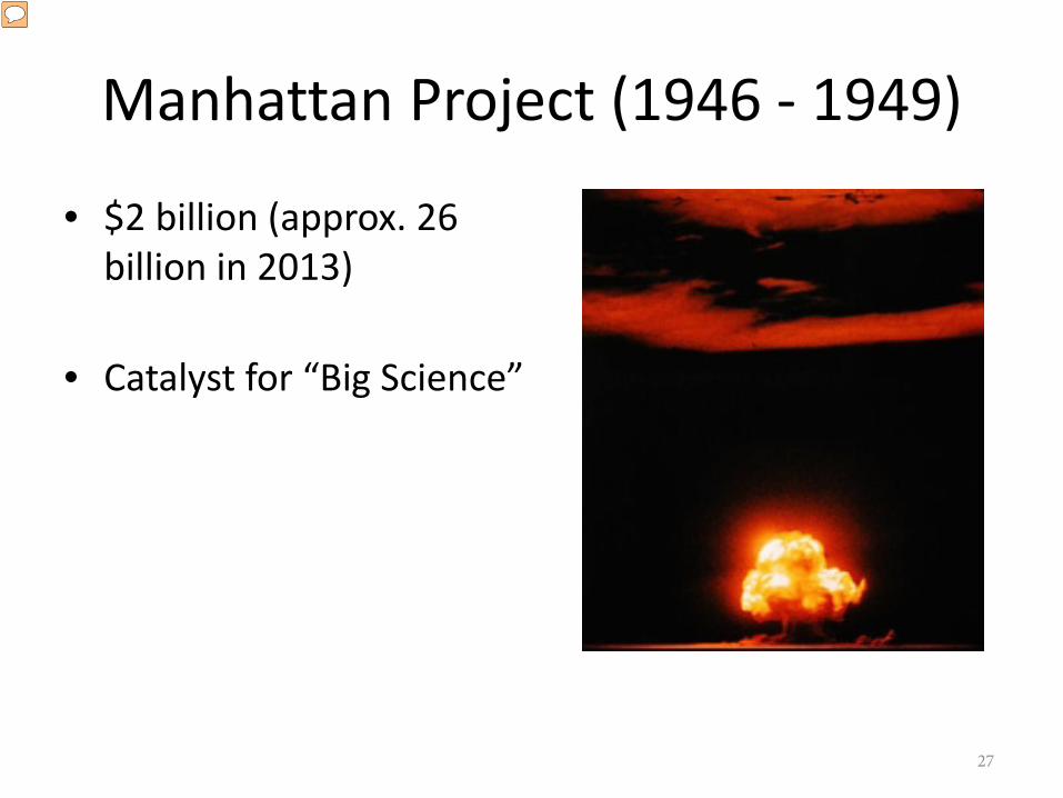
Manhattan Project (1946 - 1949)

• $2 billion (approx. 26billion in 2013)

• Catalyst for “Big Science”

27

Presenter

Presentation Notes

The next giant leap for Big Data Analytics came with the Manhattan project, the US development of the atomic bomb during World War II. The Manhattan project not only introduced the concept of Big Data analysis with computers, it was also the catalyst for Big Science

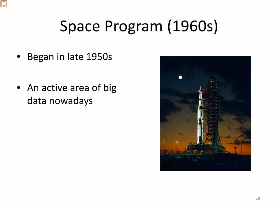
Space Program (1960s)

• Began in late 1950s

• An active area of bigdata nowadays

28

Presenter

Presentation Notes

It was driven by a Space Race between the Sovient Union and the United States, the launch of the first man-made objective to orbit the Earth, the USSR’s Sputnik 1, on 4 October 1957, the first Moon landing by the American Apollo 11 craft on 20 July 1969.

Big Science vs. Big Business

• Common– Need technologies to work with data– Use algorithms to mine data

• Big Science– Source: experiments and research conducted in

controlled environments– Goals: to answer questions, or prove theories

• Big Business– Source: transactions in nature and little control– Goals: to discover new opportunities, measure

efficiencies, uncover relationships

29

Presenter

Presentation Notes

from sources that are transactional in nature and have little control over the original of the data Use Big Data to uncover relationships among what was thought to be unrelated data sets

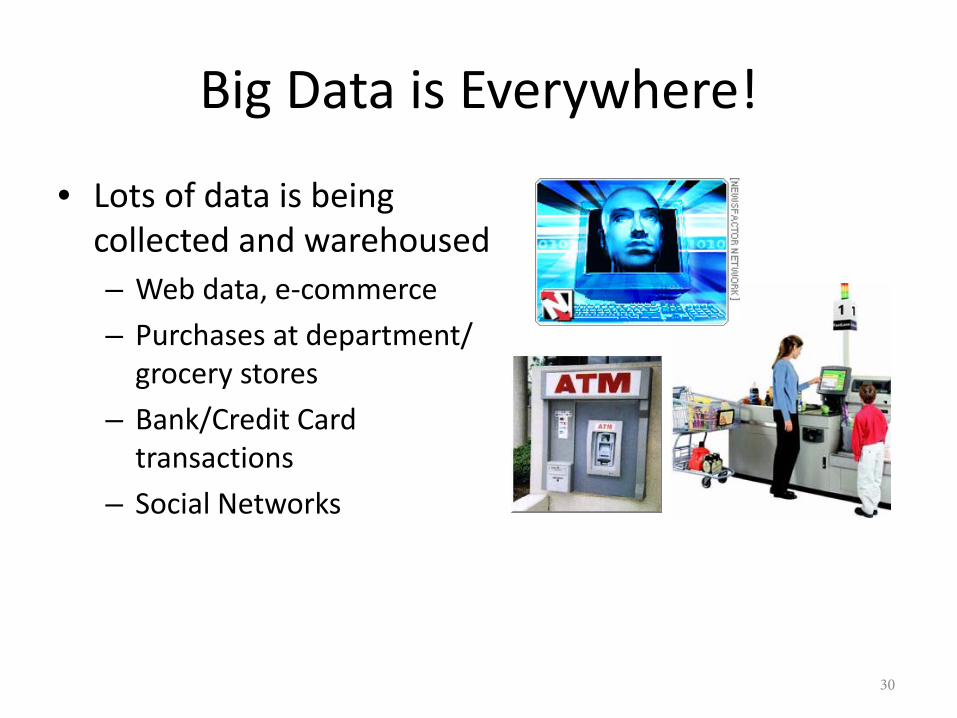
Big Data is Everywhere!

• Lots of data is beingcollected and warehoused– Web data, e-commerce– Purchases at department/

grocery stores– Bank/Credit Card

transactions– Social Networks

30

31

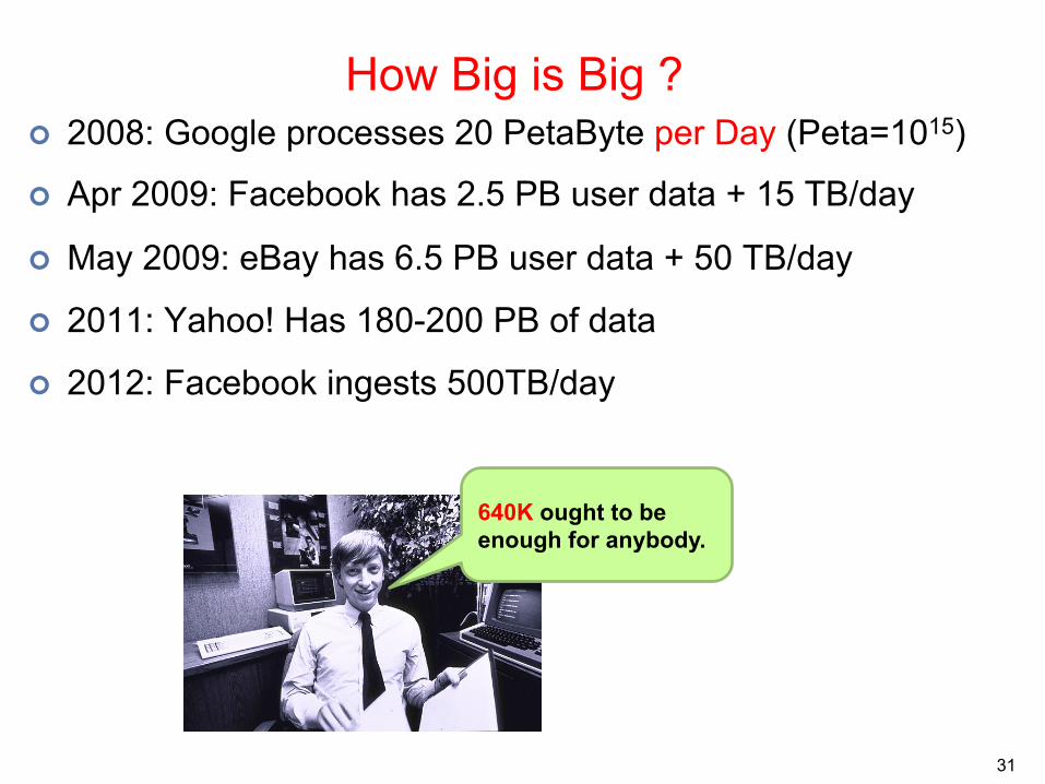
How Big is Big ? ¢  2008: Google processes 20 PetaByte per Day (Peta=1015)

¢  Apr 2009: Facebook has 2.5 PB user data + 15 TB/day

¢  May 2009: eBay has 6.5 PB user data + 50 TB/day

¢  2011: Yahoo! Has 180-200 PB of data

¢  2012: Facebook ingests 500TB/day

640K ought to be enough for anybody.

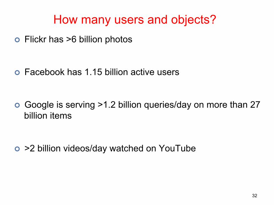
How many users and objects? ¢  Flickr has >6 billion photos

¢  Facebook has 1.15 billion active users

¢  Google is serving >1.2 billion queries/day on more than 27 billion items

¢  >2 billion videos/day watched on YouTube

32University of Pennsylvania

How much data?

¢  Modern applications use massive data: l Rendering 'Avatar' movie required >1 petabyte

of storagel eBay has >6.5 petabytes of user datal CERN's LHC will produce about 15 petabytes of

data per yearl In 2008, Google processed 20 petabytes per dayl German Climate computing center dimensioned

for 60 petabytes of climate datal Someone estimated in 2013 that Google had

10 exabytes on disk and ~ 5 exabytes on tape backupl NSA Utah Data Center is said to have 5 zettabyte (!)

¢  How much is a zettabyte? l 1,000,000,000,000,000,000,000 bytesl A stack of 1TB hard disks that is 25,400 km high

15 33

25,400 km

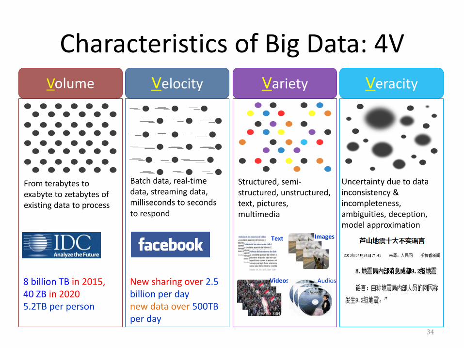
Volume VolumeVolume

Characteristics of Big Data: 4V Variety

Structured, semi-structured, unstructured, text, pictures, multimedia

Veracity

Volume

Uncertainty due to data inconsistency & incompleteness,ambiguities, deception,model approximation

Velocity

Batch data, real-time data, streaming data, milliseconds to seconds to respond

Volume

From terabytes to exabyte to zetabytes of existing data to process

Text

Videos

Images

Audios8 billion TB in 2015, 40 ZB in 20205.2TB per person

New sharing over 2.5 billion per daynew data over 500TB per day

34

How much computation?

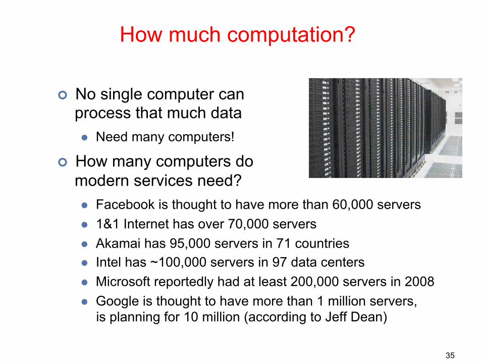
¢  No single computer can process that much data l Need many computers!

¢  How many computers do modern services need? l Facebook is thought to have more than 60,000 serversl 1&1 Internet has over 70,000 serversl Akamai has 95,000 servers in 71 countriesl Intel has ~100,000 servers in 97 data centersl Microsoft reportedly had at least 200,000 servers in 2008l Google is thought to have more than 1 million servers,

is planning for 10 million (according to Jeff Dean)

17 35 University of Pennsylvania

36

What to do with More Data ? ¢  Answering factoid questions

l Pattern matching on the Webl Works amazingly well

¢  Learning relations l Start with seed instancesl Search for patterns on the Webl Using patterns to find more instances

Who shot Abraham Lincoln? --> ??? shot Abraham Lincoln

Birthday-of(Mozart, 1756) Birthday-of(Einstein, 1879)

Wolfgang Amadeus Mozart (1756 - 1791) Einstein was born in 1879

PERSON (DATE – PERSON was born in DATE

(Brill et al., TREC 2001; Lin, ACM TOIS 2007) (Agichtein and Gravano, DL 2000; Ravichandran and Hovy, ACL 2002; … )

37

What to do with More Data ? (cont’d) Personalization

• 100-1000M users

• Spam filtering• Personalized targeting

& collaborative filtering• News recommendation• Advertising

Big Data Analytics

• Definition: A process of inspecting, cleaning,transforming, and modeling big data with thegoal of discovering useful information, suggestingconclusions, and supporting decision making

• Hot in both industrial and research societies

38

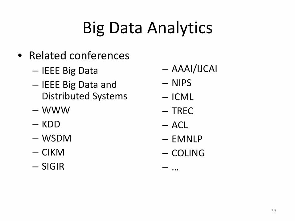
Big Data Analytics• Related conferences

– IEEE Big Data– IEEE Big Data and

Distributed Systems– WWW– KDD– WSDM– CIKM– SIGIR

– AAAI/IJCAI– NIPS– ICML– TREC– ACL– EMNLP– COLING– …

39

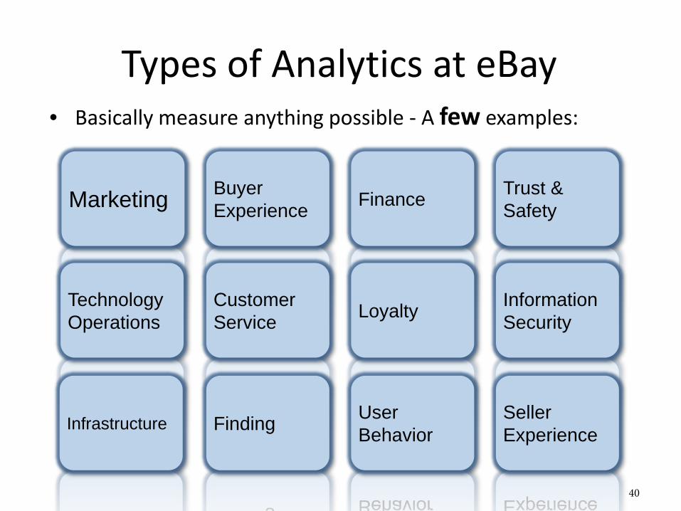
Types of Analytics at eBay• Basically measure anything possible - A few examples:

Marketing Buyer Experience Finance Trust &

Safety

Technology Operations

Customer Service Loyalty Information

Security

Infrastructure Finding User Behavior

Seller Experience

40

What is Data Mining?

• Discovery of patterns and models that are:– Valid: hold on new data with some certainty– Useful: should be possible to act on the item– Unexpected: non-obvious to the system– Understandable: humans should be able to

interpret the pattern

• A particular data analytic technique

41

42

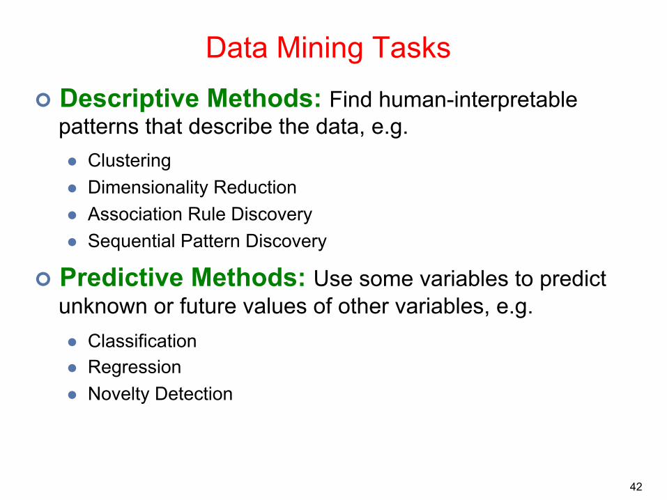
Data Mining Tasks

¢  Descriptive Methods: Find human-interpretable patterns that describe the data, e.g. l Clusteringl Dimensionality Reductionl Association Rule Discoveryl Sequential Pattern Discovery

¢  Predictive Methods: Use some variables to predict unknown or future values of other variables, e.g. l Classificationl Regressionl Novelty Detection

12/1/16

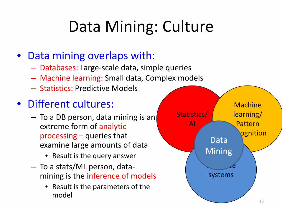
Data Mining: Culture

• Data mining overlaps with:– Databases: Large-scale data, simple queries– Machine learning: Small data, Complex models– Statistics: Predictive Models

• Different cultures:– To a DB person, data mining is an

extreme form of analyticprocessing – queries thatexamine large amounts of data

• Result is the query answer– To a stats/ML person, data-

mining is the inference of models• Result is the parameters of the

model

Statistics/AI

Machine learning/Pattern

Recognition

Database systems

Data Mining

43

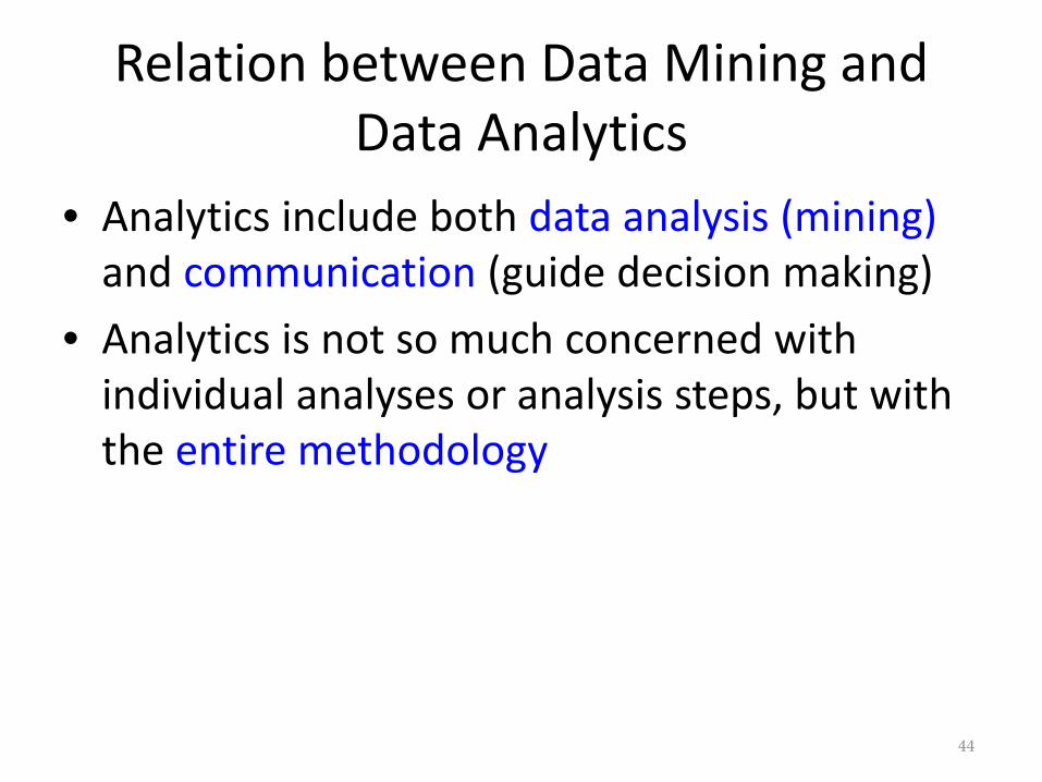
Relation between Data Mining and Data Analytics

• Analytics include both data analysis (mining)and communication (guide decision making)

• Analytics is not so much concerned withindividual analyses or analysis steps, but withthe entire methodology

44

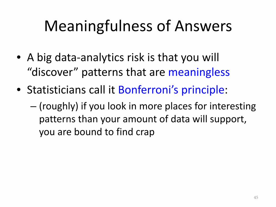
Meaningfulness of Answers

• A big data-analytics risk is that you will“discover” patterns that are meaningless

• Statisticians call it Bonferroni’s principle:– (roughly) if you look in more places for interesting

patterns than your amount of data will support,you are bound to find crap

45

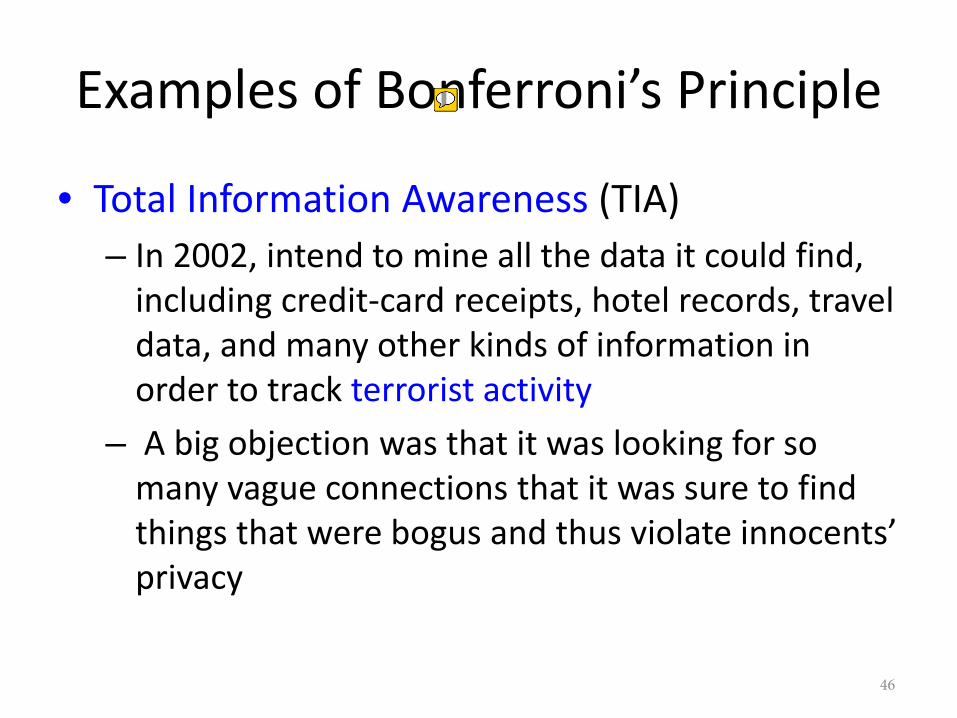
Examples of Bonferroni’s Principle

• Total Information Awareness (TIA)– In 2002, intend to mine all the data it could find,

including credit-card receipts, hotel records, traveldata, and many other kinds of information inorder to track terrorist activity

– A big objection was that it was looking for somany vague connections that it was sure to findthings that were bogus and thus violate innocents’privacy

46

huanlexu

Sticky Note

在数据随机性假设的基础上，可以计算所寻找事件出现次数的期望值。如果该结果显著高于你所希望找到的真正实例的数目，那么可以预期，寻找到的几乎任何事物都是臆造的，也就是说，它们是在统计上出现的假象，而不是你所寻找事件的凭证。上述观察现象是邦弗朗尼原理的非正式阐述。

The “TIA” Story

• Suppose we believe that certain groups ofevil-doers are meeting occasionally in hotelsto plot doing evil

• We want to find (unrelated) people who atleast twice have stayed at the same hotel onthe same day

47

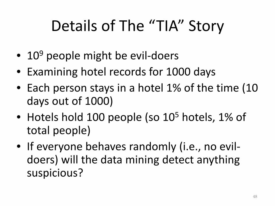
Details of The “TIA” Story

• 109 people might be evil-doers• Examining hotel records for 1000 days• Each person stays in a hotel 1% of the time (10

days out of 1000)• Hotels hold 100 people (so 105 hotels, 1% of

total people)• If everyone behaves randomly (i.e., no evil-

doers) will the data mining detect anythingsuspicious?

48

Calculation (1)

• Probability that given persons p and q will beat the same hotel on given day d:– 1/100 × 1/100 × 10-5 = 10-9.

• Probability that p and q will be at the samehotel on given days d1 and d2:– 10-9 × 10-9 = 10-18.

• Pairs of days:– 5×105

p atsomehotel

q atsomehotel Same

hotel

49

Calculation (2)

• Probability that p and q will be at the samehotel on some two days:– 5×105 × 10-18 = 5×10-13

• Pairs of people:– 5×1017

• Expected number of “suspicious” pairs ofpeople:– 5×1017 × 5×10-13 = 250,000

50

Summary of The “TIA” Story

• Suppose there are 10 pairs of evil-doers whodefinitely stayed at the same hotel twice

• Analysts have to sift through 250,000 candidatesto find the 10 real cases

• Make sure the property, e.g., two people stayedat the same hotel twice, does not allow so manypossibilities that random data will surely produce“facts of interest”

• Understanding Bonferroni’s Principle will helpyou look a little less stupid than aparapsychologist

51

In-class Practice

• Go to practice

52

Seven Typical Statistical Problems

1. Object detection(e.g. quasars): classification2. Photometric redshift estimation: regression,

conditional density estimation3. Multidimensional object discovery: querying,

dimension reduction, density estimation,clustering

4. Point-set comparison: testing and matching5. Measurement errors: errors in variables6. Extension to time domain: time series analysis7. Observation costs: active learning

53

Object Detection: Classification

54

Regression/Conditional Density Estimation

55

Querying/Dimension Reduction/Density Estimation/Clustering

56

Time Series Analysis

57

Seven Lessons in Learning from Big Data

1. Big data is a fundamental phenomenon2. The system must change3. Simple solutions run out of steam4. ML becomes important5. Data quality becomes important6. Temporal analysis become important7. Prioritized sensing becomes important

58



59



60

Current Options

1. Subsample (e.g. then use R, Weka)2. Use a simpler method (e.g. linear)3. Use brute force (e.g. Hadoop)4. Faster algorithm

61

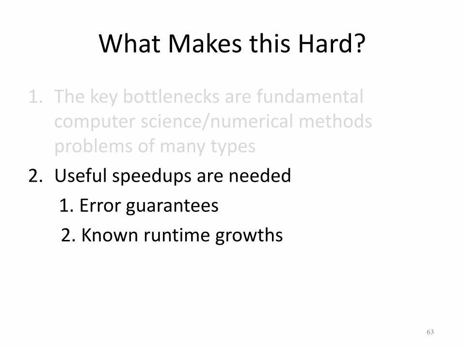
What Makes this Hard?

1. The key bottlenecks are fundamentalcomputer science/numerical methodsproblems of many types

2. Useful speedups are needed.1. Error guarantees2. Known runtime growths

62

What Makes this Hard?

1. The key bottlenecks are fundamentalcomputer science/numerical methodsproblems of many types

2. Useful speedups are needed1. Error guarantees2. Known runtime growths

63



64



65



66

Seven Typical Tasks of Machine Learning/Data Mining

1. Querying: spherical range-search O(N), orthogonal range-search O(N),nearest-neighbor O(N), all-nearest-neighbors O(N2)

2. Density estimation: mixture of Gaussians, kernel density estimationO(N2), kernel conditional density estimation O(N3)

3. Classification: decision tree, nearest-neighbor classifier O(N2), kerneldiscriminant analysis O(N2), support vector machine O(N3), Lp SVM

4. Regression: linear regression, LASSO, kernel regression O(N2), Gaussianprocess regression O(N3)

5. Dimension reduction: PCA, non-negative matrix factorization, kernelPCA O(N3), maximum variance unfolding O(N3); Gaussian graphicalmodels, discrete graphical models

6. Clustering: k-means, mean-shift O(N2), hierarchical (FoF) clusteringO(N3)

7. Testing and matching: MST O(N3), bipartite cross-matching O(N3), n-point correlation 2-sample testing O(Nn), kernel embedding

67

Seven Typical Tasks of Machine Learning/Data Mining

1. Querying: spherical range-search O(N), orthogonal range-search O(N),nearest-neighbor O(N), all-nearest-neighbors O(N2)

2. Density estimation: mixture of Gaussians, kernel density estimationO(N2), kernel conditional density estimation O(N3)

3. Classification: decision tree, nearest-neighbor classifier O(N2), kerneldiscriminant analysis O(N2), support vector machine O(N3) , Lp SVM

4. Regression: linear regression, kernel regression O(N2), Gaussian processregression O(N3), LASSO

5. Dimension reduction: PCA, non-negative matrix factorization, kernelPCA O(N3), maximum variance unfolding O(N3), Gaussian graphicalmodels, discrete graphical models

6. Clustering: k-means, mean-shift O(N2), hierarchical (FoF) clusteringO(N3)

7. Testing and matching: MST O(N3), bipartite cross-matching O(N3), n-point correlation 2-sample testing O(Nn), kernel embedding

ComputationalProblem!

67

Presenter

Presentation Notes

7 tasks of machine learning/data minging 1. Querying: spherical range-search O(N), orthogonal range-search O(N), nearest-neighbor O(N), all-nearest-neighbors O(N^2) 2. Density estimation: mixture of Gaussians, kernel density estimation O(N^2), kernel conditional density estimation O(N^3), submanifold density estimation[Grey, nips2010, O(N^3)], convex adaptive kernel estimation[Grey, AISTATS 2011, O(N^4)] 3. Classification:decision tree, nearest-neighbor classifier O(N^2), kernel discriminant analysis O(N^2), support vector machine O(N^3), LpSVM, non-negative SVM [Guan et al. ICDM 2011] 4. Regression: linear regression, LASSO, kernel regresssion O(N^2), Gaussian process regression O(N^3) 5. Dimension reduction: PCA, non-negative matrix factorizatino, kernel PCA O(N^3), maximum variance unfolding O(N^3); Gaussian graphical models, discrete graphical models, rank-preserving maps[Ouyang and Gray, ICML 2008] o(N^2); isometric separation maps [Gray, MLSP 2009] O(N^3), isometric NMF[Gray, MLSP 2009] O(N^3), functional ICA [Mehta and Gray, 2009], density preserving maps [Gray in prep] O(N^3) 6. Clustering: K-means, mean-shirt O(N^2), hierarchical (FoF) clustering O(N^3) 7. Testing and matching: MST O(N^3), bipartite cross-matching O(N^3), n-point correlation 2-sample testing O(N^n), kernel embedding

1. Divide and Conquer

• Multidimensional trees:– K-d trees [Bentley 1970], ball-trees [Omohundro 1991], spill trees [Liu,

Moore, Gray, Yang,nips2004], cover tree [Beygelzimer et al.2006] ,cosine tree [Holmes, Isbell, Gray, Nips 2009], subspace trees [Lee andGray nips 2009], cone trees [Ram and Gray kdd2012], max-margintrees [Ram and Gray SDM 2012], kernel trees [Ram and Gray]

68

http://citeseerx.ist.psu.edu/viewdoc/download?doi=10.1.1.117.8527&rep=rep1&type=pdf

http://research.microsoft.com/en-us/um/people/skakade/papers/ml/cover_tree.pdf

http://www.scopus.com/record/display.url?eid=2-s2.0-84858783218&origin=resultslist&sort=plf-f&src=s&nlo=&nlr=&nls=&sid=7DFF379FD1EE761E38ECF2CC76DC2291.kqQeWtawXauCyC8ghhRGJg:80&sot=aut&sdt=a&sl=39&s=AU-ID(%22Gray,+Alexander+G.%22+35479437600)&relp



http://siam.omnibooksonline.com/2012datamining/data/papers/038.pdf

2. Function Transforms

• Fastest approach for:– Kernel estimation (low-ish

dimension): dual-tree fastGauss transforms(multipole/Hermiteexpansions) [Lee, Gray, MooreNIPS 2005], [Lee and Gray, UAI 2006]

– KDE and GP (kernel density estimation, Gaussian process regression) (high-D): random Fourier functions [Lee and Gray, in prep]

Generalized N-body approach is fundamental:

like multidimensional generalization of FFT

69

3. Sampling• Fastest approach for (approximate):− PCA: cosine trees [Holmes, Gray, lsbell, NIPS 2008]− Kernel estimation: bandwidth learning [Holnes, Gray, lsbell, NIPS2006],[Holmes, Gray, lsbell, UAI 2007], Monte Carlo multipole method (withSVD trees) [Lee & Gray, NIPS 2009], shadow densities [Kingravi et al., underreview]−Nearest-neighbor: distance-approx., spill trees with random proj[Liu, Moore,Gray, Yang, NIPS 2004], rank-approximate: [Ram, Ouyang, Gray, NIPS 2009]

Rank-approximate NN:• Best meaning-retaining

approximation criterion in the face of high-dimensional distance

• More accurate than LSH

3. If you're going to dosampling, try smarter

(e.g. stratified) sampling

70

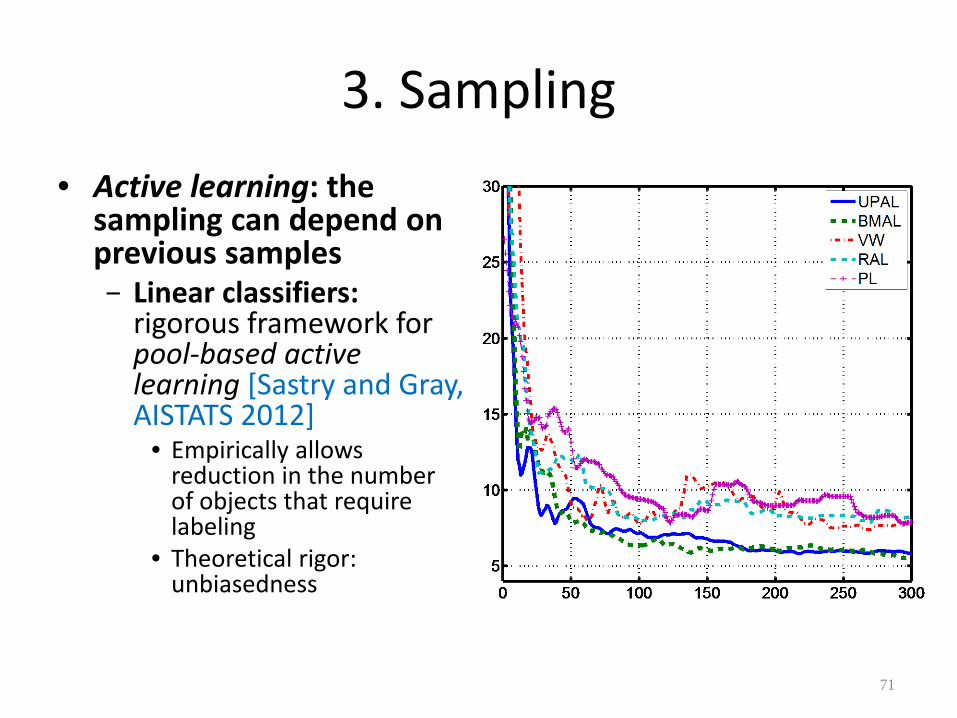
3. Sampling• Active learning: the

sampling can depend onprevious samples− Linear classifiers:

rigorous framework forpool-based activelearning [Sastry and Gray,AISTATS 2012]

• Empirically allowsreduction in the numberof objects that requirelabeling

• Theoretical rigor:unbiasedness

71

4. Caching

• Fastest approach for (using disk):− Nearest-neighbor, 2-point: Disk-based tree

algorithms in Microsoft SQL Server [Riegel, Aditya,Budavari, Gray, in prep]• Builds k-d tree on top of built-in B-trees• Fixed-pass algorithm to build k-d tree

No. of points MLDB(Dual tree) Naive

40,000 8 seconds 159 seconds

200,000 43 seconds 3480 seconds

10,000,000 297 seconds 80 hours

20,000,000 29 mins 27 sec 74 days

40,000,000 58 mins 48 sec 280 days

40,000,000 112 mins 32 sec 2 years 72

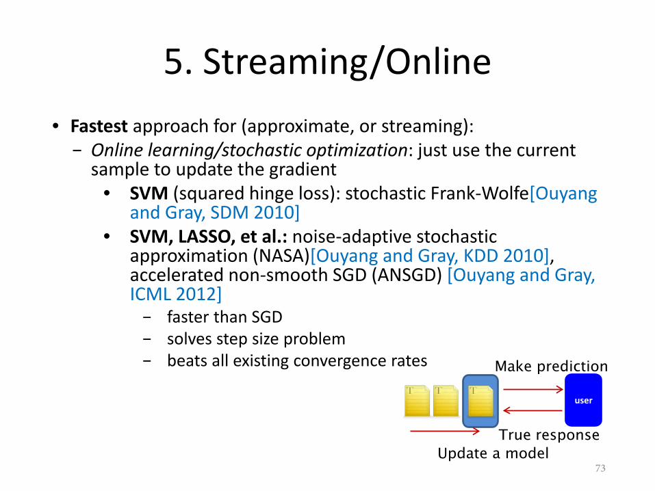
5. Streaming/Online• Fastest approach for (approximate, or streaming):

− Online learning/stochastic optimization: just use the currentsample to update the gradient

• SVM (squared hinge loss): stochastic Frank-Wolfe[Ouyangand Gray, SDM 2010]

• SVM, LASSO, et al.: noise-adaptive stochasticapproximation (NASA)[Ouyang and Gray, KDD 2010],accelerated non-smooth SGD (ANSGD) [Ouyang and Gray,ICML 2012]− faster than SGD− solves step size problem− beats all existing convergence rates

Update a modelTrue response

user

Make prediction

73

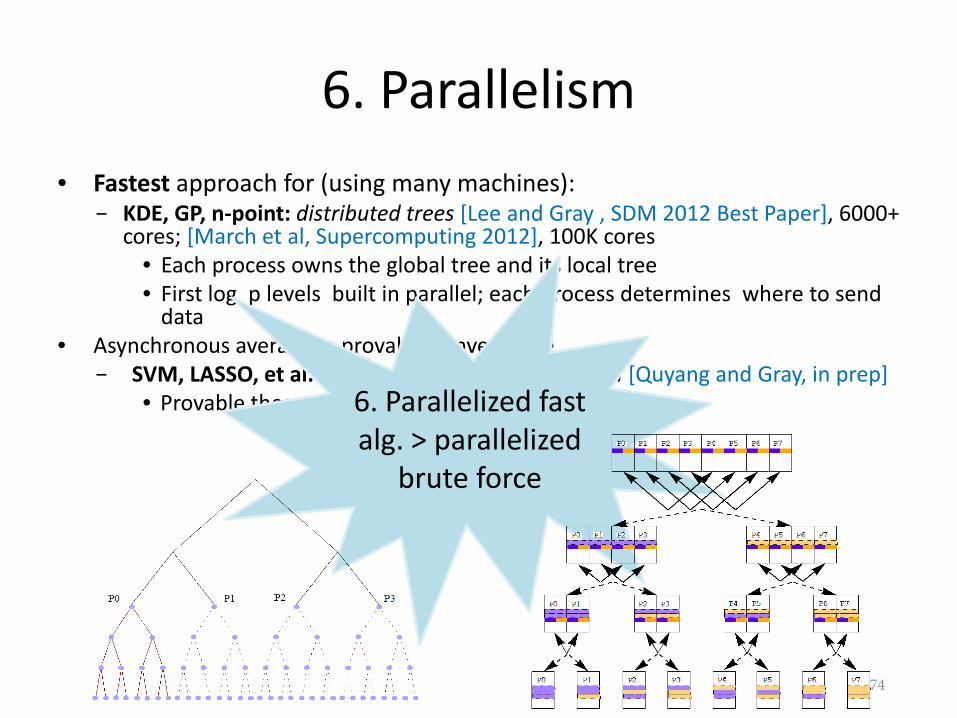
• Fastest approach for (using many machines):− KDE, GP, n-point: distributed trees [Lee and Gray , SDM 2012 Best Paper], 6000+

cores; [March et al, Supercomputing 2012], 100K cores• Each process owns the global tree and its local tree• First log p levels built in parallel; each process determines where to send

data• Asynchronous averaging; provable convergence

− SVM, LASSO, et al.: distributed online optimization [Quyang and Gray, in prep]• Provable theoretical speed up for the first time6. Parallelized fast

alg. > parallelized brute force

6. Parallelism

74

7. Transformations between Problems

• Change the problem type:− Linear algebra on kernel matrices N-body inside conjugate

gradient [Gray, TR 2004]− Euclidean graphs N-body problems [March & Gray, KDD 2010]− HMM as graphmatrix factorization [Tran & Gray, in prep]

• Optimizations: reformulate the objective and constraints:− Maximum variance unfolding: SDP via Burer-Monteiro convex

relaxation [Vasiloglou, Gray, Anderson MLSP 2009]− Lq SVM, 0<q<1: DC programming [Guan & Gray, CSDA 2-11]− L0 SVM: mixed integer nonlinear program via perspective cuts

[Guan & Gray, under review]− Do reformulations automatically [Agarwal et al, PADL 2010],[Bhat

et al, POPL 2012]

75

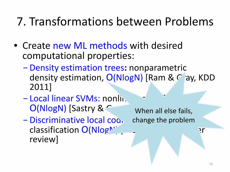
7. Transformations between Problems

• Create new ML methods with desiredcomputational properties:− Density estimation trees: nonparametric

density estimation, O(NlogN) [Ram & Gray, KDD2011]

− Local linear SVMs: nonlinear classification,O(NlogN) [Sastry & Gray, under review]

− Discriminative local coding: nonlinear classification O(NlogN) [Mehta & Gray, under review]

When all else fails, change the problem

76

77

What is cloud computing?

78

The best thing since sliced bread? ¢  Before clouds…

l Gridsl Vector supercomputersl …

¢  Cloud computing means many different things: l Large-data processingl Rebranding of web 2.0l Utility computingl Everything as a service

79

Rebranding of web 2.0 ¢  Rich, interactive web applications

l Clouds refer to the servers that run theml AJAX as the de facto standard (for better or worse)l Examples: Facebook, YouTube, Gmail, …

¢  “The network is the computer”: take two l User data is stored “in the clouds”l Rise of the netbook, smartphones, etc.l Browser is the OS

80

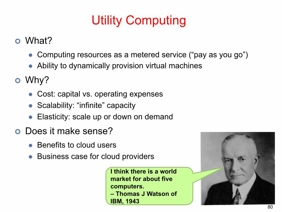
Utility Computing ¢  What?

l Computing resources as a metered service (“pay as you go”)l Ability to dynamically provision virtual machines

¢  Why? l Cost: capital vs. operating expensesl Scalability: “infinite” capacityl Elasticity: scale up or down on demand

¢  Does it make sense? l Benefits to cloud usersl Business case for cloud providers

I think there is a world market for about five computers. – Thomas J Watson ofIBM, 1943

81

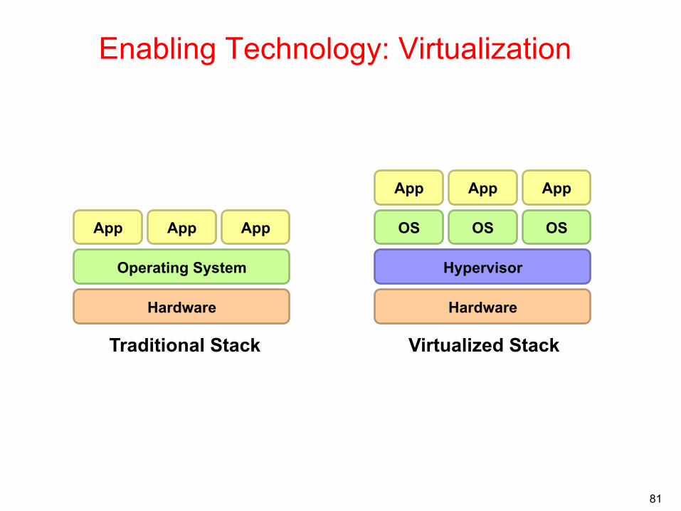
Enabling Technology: Virtualization

Hardware

Operating System

App App App

Traditional Stack

Hardware

OS

App App App

Hypervisor

OS OS

Virtualized Stack

82

Everything as a Service ¢  Utility computing = Infrastructure as a Service (IaaS)

l Why buy machines when you can rent cycles?l Examples: Amazon’s EC2, Rackspace

¢  Platform as a Service (PaaS) l Give me nice API and take care of the maintenance, upgrades, …l Example: Google App Engine

¢  Software as a Service (SaaS) l Just run it for me!l Example: Gmail, Salesforce

83

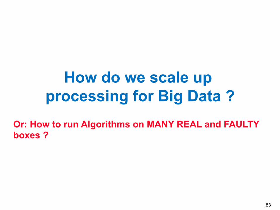
How do we scale up processing for Big Data ?

Or: How to run Algorithms on MANY REAL and FAULTY boxes ?

84

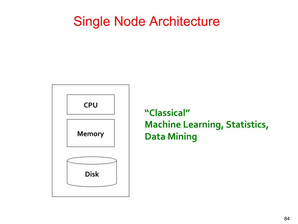
Single Node Architecture

12/1/16

Memory

Disk

CPU “Classical” Machine Learning, Statistics, Data Mining

85

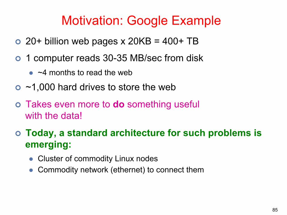
Motivation: Google Example ¢  20+ billion web pages x 20KB = 400+ TB

¢  1 computer reads 30-35 MB/sec from disk l ~4 months to read the web

¢  ~1,000 hard drives to store the web

¢  Takes even more to do something useful with the data!

¢  Today, a standard architecture for such problems is emerging: l Cluster of commodity Linux nodesl Commodity network (ethernet) to connect them

12/1/16

Mem

Disk

CPU

Mem

Disk

CPU

…

Switch

Each rack contains 16-64 nodes

Mem

Disk

CPU

Mem

Disk

CPU

…

Switch

Switch 1 Gbps between any pair of nodes in a rack

2-10 Gbps backbone between racks

In 2011, it was guestimated that Google had 1M machines, http://bit.ly/Shh0RO

Overview 57 12/1/16 57

88

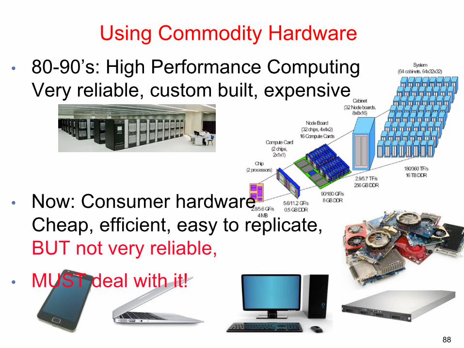
Using Commodity Hardware • 80-90’s: High Performance Computing

Very reliable, custom built, expensive

• Now: Consumer hardwareCheap, efficient, easy to replicate,BUT not very reliable,

• MUST deal with it!

89

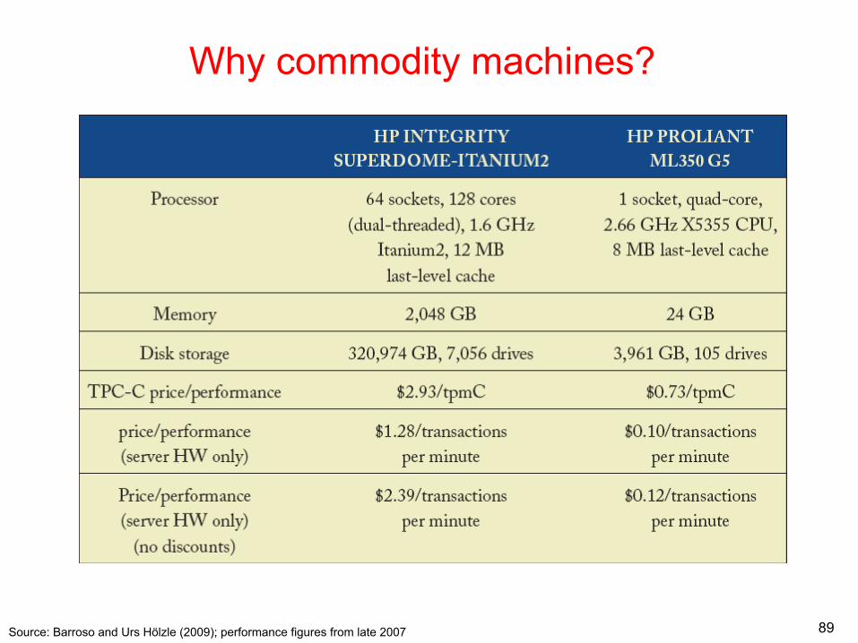
Why commodity machines?

Source: Barroso and Urs Hölzle (2009); performance figures from late 2007

90

• Performance goal• 1 failure per year• for a 1000-machine Cluster

• Poisson approximation

• Assume failure rate per machine• Poisson rates of independent random variables are additive,

so we can combine=> With Fault Intolerant Engineering We need a rate of 1 failure per 1000 years per machine • Fault tolerance

Assume we can tolerate k faults among m machines in t time

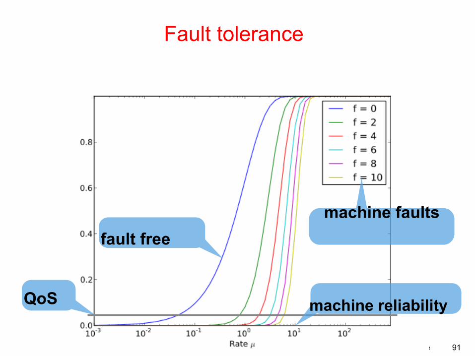
Fault Tolerance

not IBM Deskstar!

Ove 91

Fault tolerance

machine faults

QoS machine reliability

fault free

92

Advantages of scaling “out”

So why not?

In-class Practice

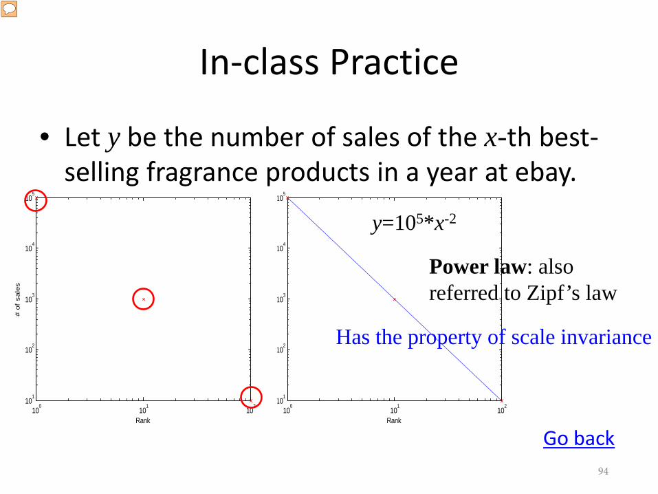
• Let us examine fragrance sales at ebay in ayear. Suppose– the best selling product sold 100,000 pieces,– the 10th best-selling product sold 1,000 pieces,– the 100th best selling product sold 10 pieces.

• How to derive the relationship between thenumber of fragrance sold and the order?

93

100

101

102

101

102

103

104

105

Rank

# of

sal

es

100

101

102

101

102

103

104

105

Rank

# of

sal

es

In-class Practice

• Let y be the number of sales of the x-th best-selling fragrance products in a year at ebay.

y=105*x-2

Power law: also referred to Zipf’s law

Has the property of scale invariance

Go back94

Presenter

Presentation Notes

scaling by a constant c simply multiplies the original power-law relation by the constant c^k

lecture 1: introduction and motivation - xuhappy.github.io · motivation of the course • do you...

Documents