lecture 1: reproducibility of science: impact of bayesian
TRANSCRIPT
CBMS: Model Uncertainty and Multiplicity Santa Cruz, July 23-28, 2012'
&
$
%
Lecture 1: Reproducibility of Science:Impact of Bayesian Testing and Multiplicity
Jim Berger
Duke University
CBMS Conference on Model Uncertainty and MultiplicityJuly 23-28, 2012
1
CBMS: Model Uncertainty and Multiplicity Santa Cruz, July 23-28, 2012'
&
$
%
Outline• I. Reproducibility of Science
– Evidence of an increasing lack of reproducibility of science
– Some reasons for the lack of reproducibility
∗ Publication bias
∗ Experimental biases, including programming errors
∗ The very considerable rewards for ‘positive’ results
∗ Statistical biases
∗ Egregiously bad statistics
∗ The incorrect way in which p-values are used
∗ Failure to adjust for multiplicities
· Multiple testing
· Multiple looks at the data
· Multiple statistical analyses
– How Bayesian analysis can help
• II. A Brief History of Bayesian Statistics
• III. Could Fisher, Jeffreys and Neyman have agreed on testing?
2
CBMS: Model Uncertainty and Multiplicity Santa Cruz, July 23-28, 2012'
&
$
%
I. Reproducibility of Science
A. Evidence for a Lack of Reproducibility
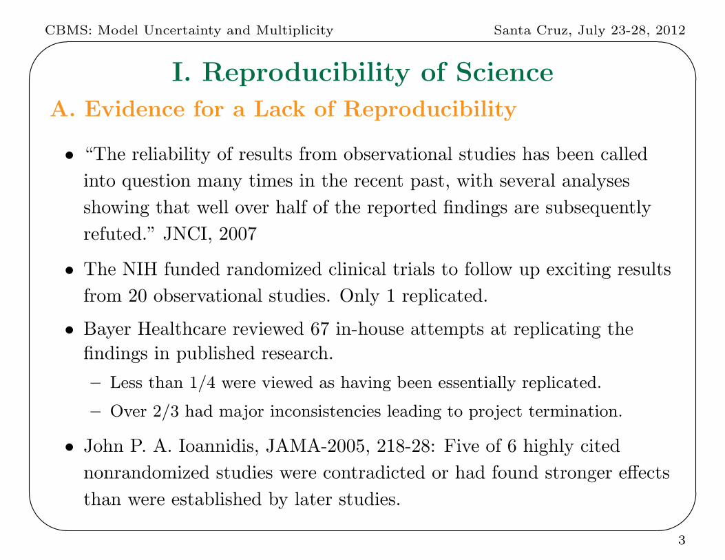
• “The reliability of results from observational studies has been called
into question many times in the recent past, with several analyses
showing that well over half of the reported findings are subsequently
refuted.” JNCI, 2007
• The NIH funded randomized clinical trials to follow up exciting results
from 20 observational studies. Only 1 replicated.
• Bayer Healthcare reviewed 67 in-house attempts at replicating the
findings in published research.
– Less than 1/4 were viewed as having been essentially replicated.
– Over 2/3 had major inconsistencies leading to project termination.
• John P. A. Ioannidis, JAMA-2005, 218-28: Five of 6 highly cited
nonrandomized studies were contradicted or had found stronger effects
than were established by later studies.
3

CBMS: Model Uncertainty and Multiplicity Santa Cruz, July 23-28, 2012'
&
$
%
Even the best studies often fail to replicate.
• Ioannidis looked at the 49 most famous medical publications from
1990-2003 resulting from randomized trials; 45 claimed successful
intervention.
– 7 (16%) were contradicted by subsequent studies
– 7 others (16%) had found effects that were stronger than those of
subsequent studies
– 20 (44%) were replicated
– 11 (24%) remained largely unchallenged.
• Phase II drug trials success rates are falling (28% 5 years ago, 18%
now) (Arrowsmith (2011) Nature Reviews Drug Discovery 10)
• 50% phase III drug trial failure rates are now being reported, versus a
20% failure rate 10 years ago (Arrowsmith (2011) Nature Reviews Drug
Discovery 10); 70% phase III cancer drug failure rate
• Reports that 30% of phase III drug trial successes fail to replicate
4
CBMS: Model Uncertainty and Multiplicity Santa Cruz, July 23-28, 2012'
&
$
%
B. Some Reasons for a Lack of Reproducibility
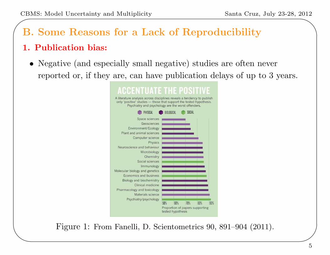
1. Publication bias:
• Negative (and especially small negative) studies are often never
reported or, if they are, can have publication delays of up to 3 years.
Figure 1: From Fanelli, D. Scientometrics 90, 891–904 (2011).
5
CBMS: Model Uncertainty and Multiplicity Santa Cruz, July 23-28, 2012'
&
$
%
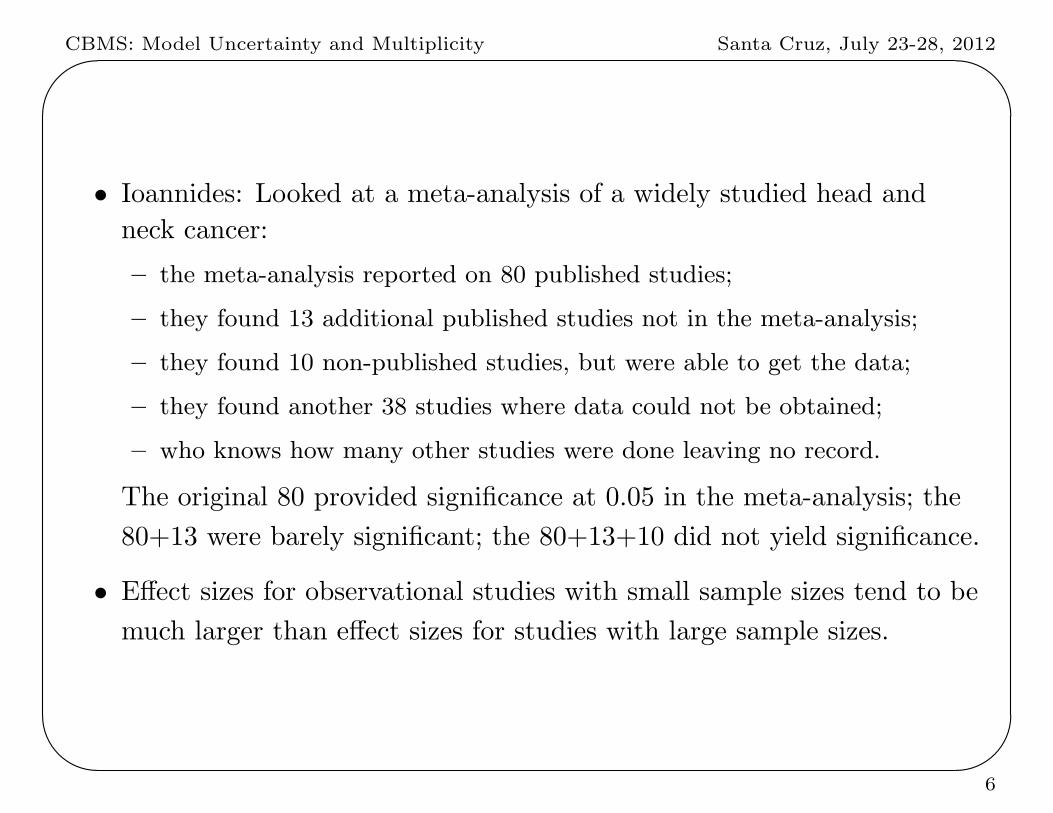
• Ioannides: Looked at a meta-analysis of a widely studied head and
neck cancer:
– the meta-analysis reported on 80 published studies;
– they found 13 additional published studies not in the meta-analysis;
– they found 10 non-published studies, but were able to get the data;
– they found another 38 studies where data could not be obtained;
– who knows how many other studies were done leaving no record.
The original 80 provided significance at 0.05 in the meta-analysis; the
80+13 were barely significant; the 80+13+10 did not yield significance.
• Effect sizes for observational studies with small sample sizes tend to be
much larger than effect sizes for studies with large sample sizes.
6

CBMS: Model Uncertainty and Multiplicity Santa Cruz, July 23-28, 2012'
&
$
%
• Interesting approach to detecting bias (Ioannides and Trikalinos, 2007):
– look at the available studies, focusing on sample sizes and effect sizes;
– perform a meta-analysis to estimate the overall effect;
– simulate studies from this assumed population effect and the same sample
sizes to determine how many studies should be nonsignificant, and
compare this with the actual number of nonsignificant studies.
Examples (Gregory Francis, Psychon Bull Rev, 2012):
• The probability having one or fewer non-significant studies in the ten Bem
(2011) psi* experiments is 0.058.
• Meissner & Brigham (2001) performed a meta-analysis of 18 experiments on
verbal overshadowing**, nine of which were significant. The probability of
nine or fewer non-significant experiments is 0.022 (1:5 odds)
Note: If there were publication bias, this would underestimate its extent, because
of using the published studies to determine the overall effect.
*sensing future events and using that information to judge the present
**visual memory is impaired after subjects give a verbal description of the stimuli
7
CBMS: Model Uncertainty and Multiplicity Santa Cruz, July 23-28, 2012'
&
$
%
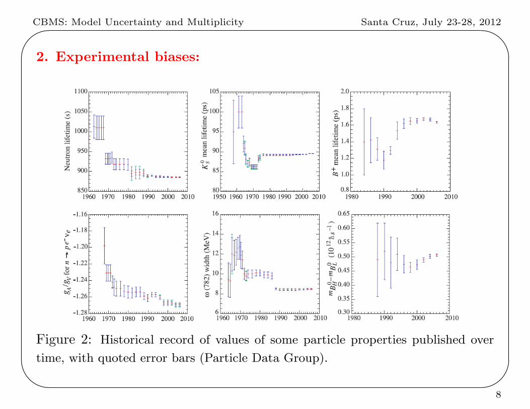
2. Experimental biases:
Figure 2: Historical record of values of some particle properties published over
time, with quoted error bars (Particle Data Group).
8
CBMS: Model Uncertainty and Multiplicity Santa Cruz, July 23-28, 2012'
&
$
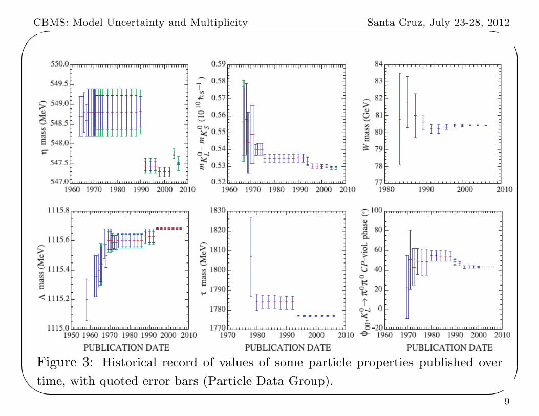
%Figure 3: Historical record of values of some particle properties published over
time, with quoted error bars (Particle Data Group).
9

CBMS: Model Uncertainty and Multiplicity Santa Cruz, July 23-28, 2012'
&
$
%
3. The very considerable rewards for ‘positive’ results
• Money and fame
– “There is nothing wrong with cancer research that a little less money
wouldn’t cure.” (Nathan Mantel, NCI)
• Promotion and tenure
• Journals want high impact factors
• ...
• And, except perhaps for physics, there seems to be little to no scientific
penalty for having a positive finding later refuted.
10

CBMS: Model Uncertainty and Multiplicity Santa Cruz, July 23-28, 2012'
&
$
%
4. Statistical biases
• Confounding, especially in observational studies
– Worse with large sample sizes
• Programming errors
“To err is human, but to really foul things up requires a computer.”
Farmers’ Almanac (1978)
• ...
11
CBMS: Model Uncertainty and Multiplicity Santa Cruz, July 23-28, 2012'
&
$
%
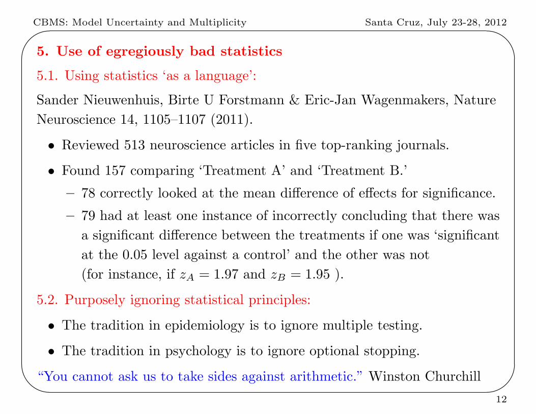
5. Use of egregiously bad statistics
5.1. Using statistics ‘as a language’:
Sander Nieuwenhuis, Birte U Forstmann & Eric-Jan Wagenmakers, Nature
Neuroscience 14, 1105–1107 (2011).
• Reviewed 513 neuroscience articles in five top-ranking journals.
• Found 157 comparing ‘Treatment A’ and ‘Treatment B.’
– 78 correctly looked at the mean difference of effects for significance.
– 79 had at least one instance of incorrectly concluding that there was
a significant difference between the treatments if one was ‘significant
at the 0.05 level against a control’ and the other was not
(for instance, if zA = 1.97 and zB = 1.95 ).
5.2. Purposely ignoring statistical principles:
• The tradition in epidemiology is to ignore multiple testing.
• The tradition in psychology is to ignore optional stopping.
“You cannot ask us to take sides against arithmetic.” Winston Churchill
12
CBMS: Model Uncertainty and Multiplicity Santa Cruz, July 23-28, 2012'
&
$
%
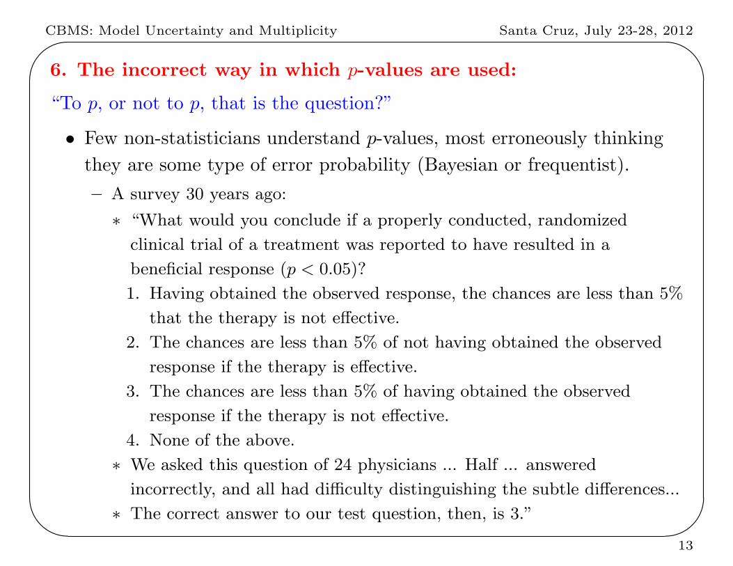
6. The incorrect way in which p-values are used:
“To p, or not to p, that is the question?”
• Few non-statisticians understand p-values, most erroneously thinking
they are some type of error probability (Bayesian or frequentist).
– A survey 30 years ago:
∗ “What would you conclude if a properly conducted, randomized
clinical trial of a treatment was reported to have resulted in a
beneficial response (p < 0.05)?
1. Having obtained the observed response, the chances are less than 5%
that the therapy is not effective.
2. The chances are less than 5% of not having obtained the observed
response if the therapy is effective.
3. The chances are less than 5% of having obtained the observed
response if the therapy is not effective.
4. None of the above.
∗ We asked this question of 24 physicians ... Half ... answered
incorrectly, and all had difficulty distinguishing the subtle differences...
∗ The correct answer to our test question, then, is 3.”
13

CBMS: Model Uncertainty and Multiplicity Santa Cruz, July 23-28, 2012'
&
$
%
“This isn’t right. This isn’t even wrong.” –Wolfgang Pauli, on a
submitted paper
∗ Actual correct answer: The chances are less than 5% of having
obtained the observed response or any more extreme response if
the therapy is not effective.
• But, is it fair to count ‘possible data more extreme than the actual
data’ in the evidence against the null hypothesis?
Jeffreys (1961): “An hypothesis, that may be true, may be rejected
because it has not predicted observable results that have not occurred.”
• Matthews (1998): “The plain fact is that 70 years ago Ronald Fisher
gave scientists a mathematical machine for turning baloney into
breakthroughs, and flukes into funding.”
• When testing precise hypotheses, true error probabilities (Bayesian or
frequentist) are much larger than p-values.
– Later examples.
– Applet (of German Molina) available at www.stat.duke.edu/∼berger
14

CBMS: Model Uncertainty and Multiplicity Santa Cruz, July 23-28, 2012'
&
$
%
7. Failure to adjust for multiplicities:
• Failure to properly account for multiple testing:
– In a recent talk about the drug discovery process, the following numbers
were given in illustration.
∗ 10,000 relevant compounds were screened for biological activity.
∗ 500 passed the initial screen and were studied in vitro.
∗ 25 passed this screening and were studied in Phase I animal trials.
∗ 1 passed this screening and was studied in a Phase II human trial.
This could be nothing but noise, if screening was done based on
‘significance at the 0.05 level.’
“Basic research is like shooting an arrow in the air and, where it lands,
painting a target.” Homer Adkins
– Multiple Multiple Testing (e.g., plasma samples are sent to separate
genomic, protein, and metabolic labs for ‘discovery’.)
– Serial Studies (e.g., there have been 16 large Phase III Alzheimer’s trials -
all failing; the probability of that is 0.44)
– The tradition in epidemiology is to ignore multiple testing,
∗ usually arguing that the purpose is to find anomalies for further study.
15
CBMS: Model Uncertainty and Multiplicity Santa Cruz, July 23-28, 2012'
&
$
%
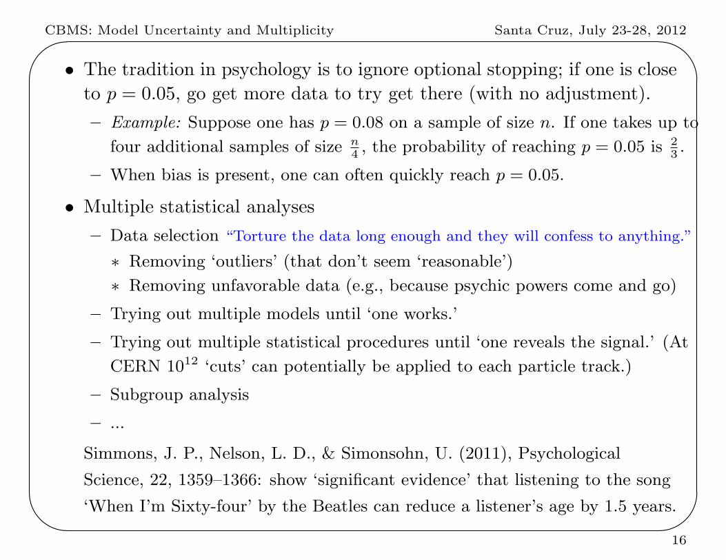
• The tradition in psychology is to ignore optional stopping; if one is close
to p = 0.05, go get more data to try get there (with no adjustment).
– Example: Suppose one has p = 0.08 on a sample of size n. If one takes up to
four additional samples of size n4, the probability of reaching p = 0.05 is 2
3.
– When bias is present, one can often quickly reach p = 0.05.
• Multiple statistical analyses
– Data selection “Torture the data long enough and they will confess to anything.”
∗ Removing ‘outliers’ (that don’t seem ‘reasonable’)
∗ Removing unfavorable data (e.g., because psychic powers come and go)
– Trying out multiple models until ‘one works.’
– Trying out multiple statistical procedures until ‘one reveals the signal.’ (At
CERN 1012 ‘cuts’ can potentially be applied to each particle track.)
– Subgroup analysis
– ...
Simmons, J. P., Nelson, L. D., & Simonsohn, U. (2011), Psychological
Science, 22, 1359–1366: show ‘significant evidence’ that listening to the song
‘When I’m Sixty-four’ by the Beatles can reduce a listener’s age by 1.5 years.
16
CBMS: Model Uncertainty and Multiplicity Santa Cruz, July 23-28, 2012'
&
$
%
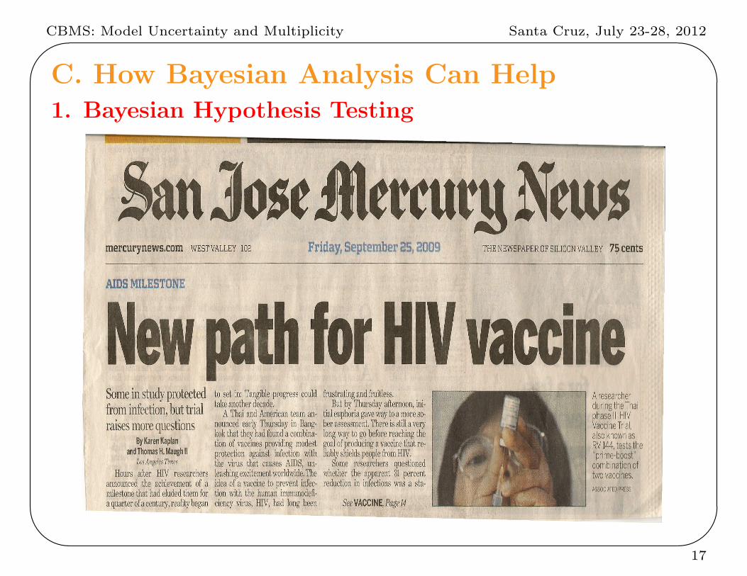
C. How Bayesian Analysis Can Help1. Bayesian Hypothesis Testing
17
CBMS: Model Uncertainty and Multiplicity Santa Cruz, July 23-28, 2012'
&
$
%
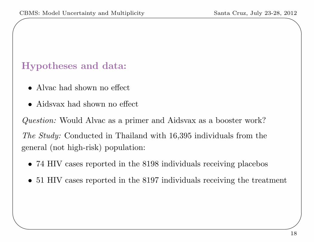
Hypotheses and data:
• Alvac had shown no effect
• Aidsvax had shown no effect
Question: Would Alvac as a primer and Aidsvax as a booster work?
The Study: Conducted in Thailand with 16,395 individuals from the
general (not high-risk) population:
• 74 HIV cases reported in the 8198 individuals receiving placebos
• 51 HIV cases reported in the 8197 individuals receiving the treatment
18
CBMS: Model Uncertainty and Multiplicity Santa Cruz, July 23-28, 2012'
&
$
%
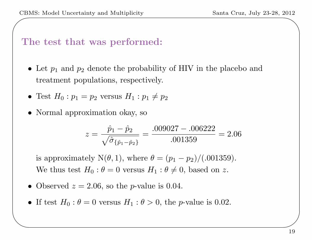
The test that was performed:
• Let p1 and p2 denote the probability of HIV in the placebo and
treatment populations, respectively.
• Test H0 : p1 = p2 versus H1 : p1 = p2
• Normal approximation okay, so
z =p1 − p2√σp1−p2
=.009027− .006222
.001359= 2.06
is approximately N(θ, 1), where θ = (p1 − p2)/(.001359).
We thus test H0 : θ = 0 versus H1 : θ = 0, based on z.
• Observed z = 2.06, so the p-value is 0.04.
• If test H0 : θ = 0 versus H1 : θ > 0, the p-value is 0.02.
19
CBMS: Model Uncertainty and Multiplicity Santa Cruz, July 23-28, 2012'
&
$
%
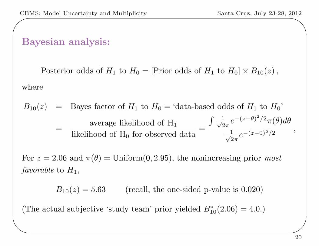
Bayesian analysis:
Posterior odds of H1 to H0 = [Prior odds of H1 to H0]×B10(z) ,
where
B10(z) = Bayes factor of H1 to H0 = ‘data-based odds of H1 to H0’
=average likelihood of H1
likelihood of H0 for observed data=
∫1√2π
e−(z−θ)2/2π(θ)dθ
1√2π
e−(z−0)2/2,
For z = 2.06 and π(θ) = Uniform(0, 2.95), the nonincreasing prior most
favorable to H1,
B10(z) = 5.63 (recall, the one-sided p-value is 0.020)
(The actual subjective ‘study team’ prior yielded B∗10(2.06) = 4.0.)
20
CBMS: Model Uncertainty and Multiplicity Santa Cruz, July 23-28, 2012'
&
$
%
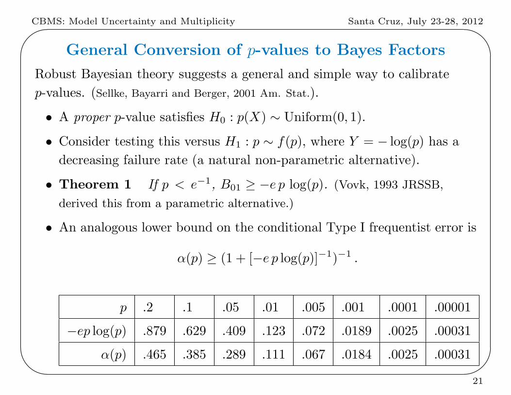
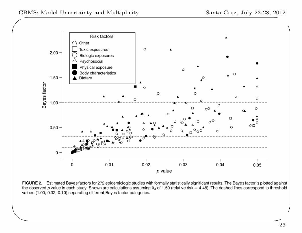
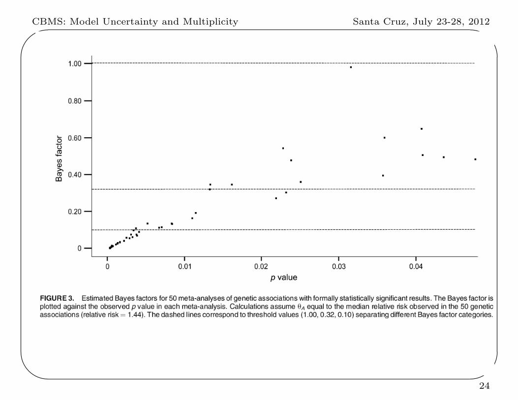
General Conversion of p-values to Bayes Factors
Robust Bayesian theory suggests a general and simple way to calibrate
p-values. (Sellke, Bayarri and Berger, 2001 Am. Stat.).
• A proper p-value satisfies H0 : p(X) ∼ Uniform(0, 1).
• Consider testing this versus H1 : p ∼ f(p), where Y = − log(p) has a
decreasing failure rate (a natural non-parametric alternative).
• Theorem 1 If p < e−1, B01 ≥ −e p log(p). (Vovk, 1993 JRSSB,
derived this from a parametric alternative.)
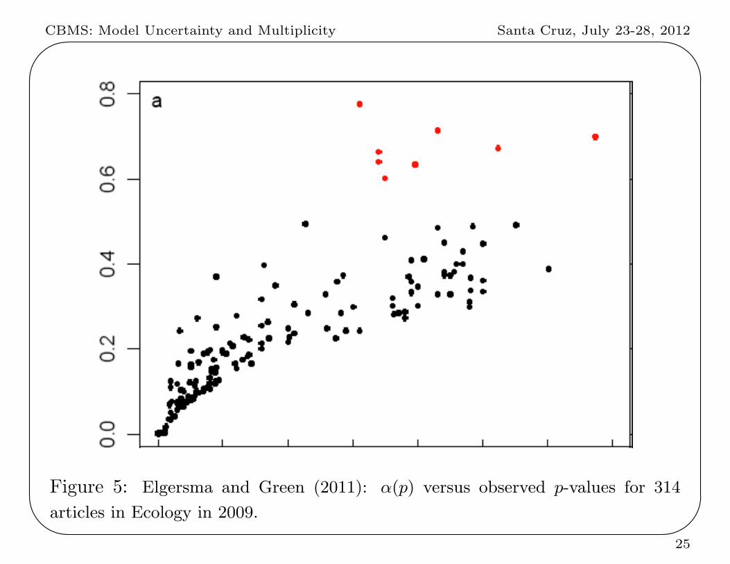
• An analogous lower bound on the conditional Type I frequentist error is
α(p) ≥ (1 + [−e p log(p)]−1)−1 .
p .2 .1 .05 .01 .005 .001 .0001 .00001
−ep log(p) .879 .629 .409 .123 .072 .0189 .0025 .00031
α(p) .465 .385 .289 .111 .067 .0184 .0025 .00031
21
CBMS: Model Uncertainty and Multiplicity Santa Cruz, July 23-28, 2012'
&
$
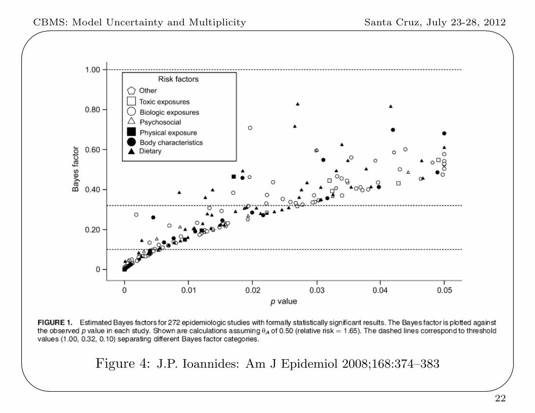
%Figure 4: J.P. Ioannides: Am J Epidemiol 2008;168:374–383
22
CBMS: Model Uncertainty and Multiplicity Santa Cruz, July 23-28, 2012'
&
$
%23
CBMS: Model Uncertainty and Multiplicity Santa Cruz, July 23-28, 2012'
&
$
%24
CBMS: Model Uncertainty and Multiplicity Santa Cruz, July 23-28, 2012'
&
$
%Figure 5: Elgersma and Green (2011): α(p) versus observed p-values for 314
articles in Ecology in 2009.
25
CBMS: Model Uncertainty and Multiplicity Santa Cruz, July 23-28, 2012'
&
$
%
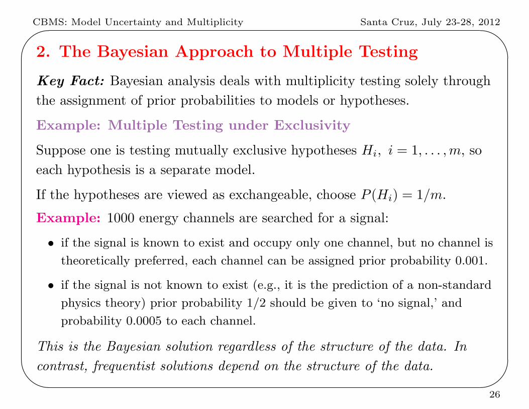
2. The Bayesian Approach to Multiple Testing
Key Fact: Bayesian analysis deals with multiplicity testing solely through
the assignment of prior probabilities to models or hypotheses.
Example: Multiple Testing under Exclusivity
Suppose one is testing mutually exclusive hypotheses Hi, i = 1, . . . ,m, so
each hypothesis is a separate model.
If the hypotheses are viewed as exchangeable, choose P (Hi) = 1/m.
Example: 1000 energy channels are searched for a signal:
• if the signal is known to exist and occupy only one channel, but no channel is
theoretically preferred, each channel can be assigned prior probability 0.001.
• if the signal is not known to exist (e.g., it is the prediction of a non-standard
physics theory) prior probability 1/2 should be given to ‘no signal,’ and
probability 0.0005 to each channel.
This is the Bayesian solution regardless of the structure of the data. In
contrast, frequentist solutions depend on the structure of the data.
26
CBMS: Model Uncertainty and Multiplicity Santa Cruz, July 23-28, 2012'
&
$
%
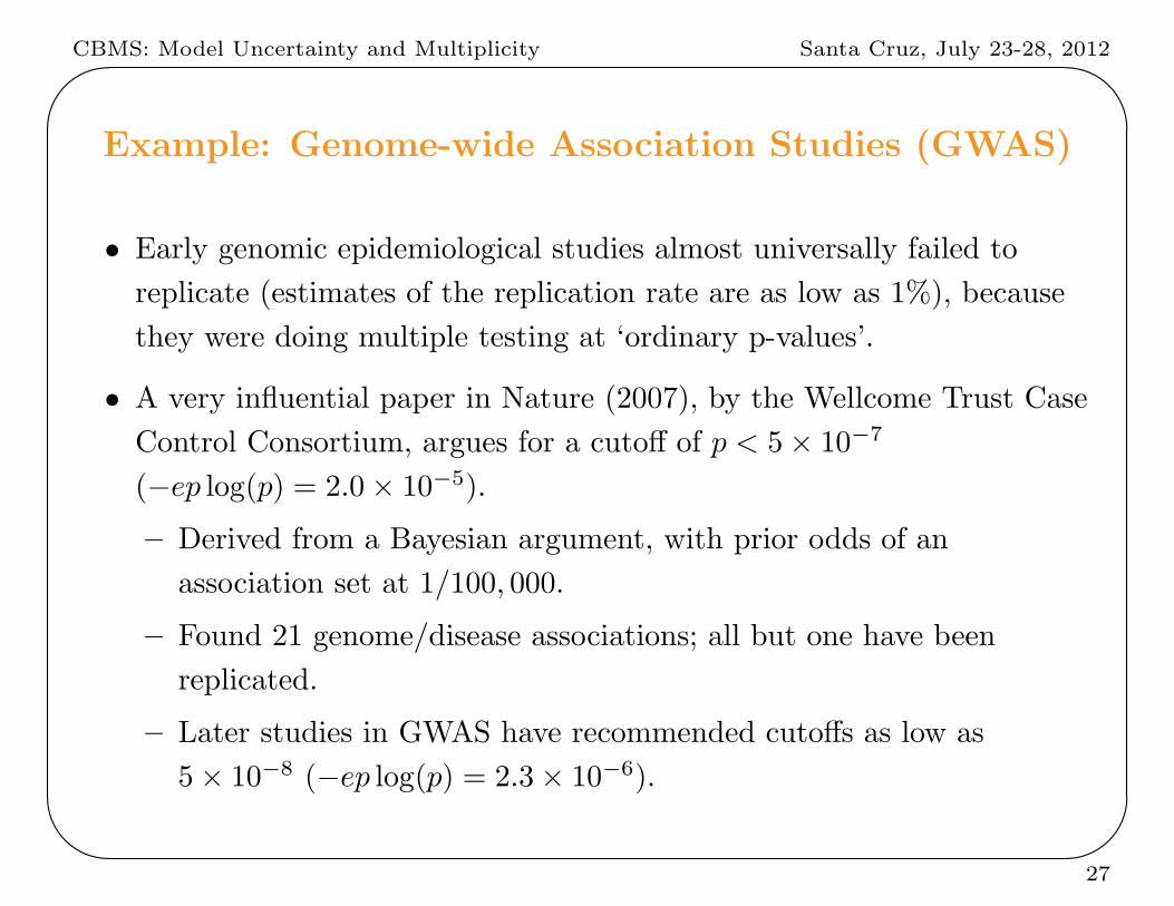
Example: Genome-wide Association Studies (GWAS)
• Early genomic epidemiological studies almost universally failed to
replicate (estimates of the replication rate are as low as 1%), because
they were doing multiple testing at ‘ordinary p-values’.
• A very influential paper in Nature (2007), by the Wellcome Trust Case
Control Consortium, argues for a cutoff of p < 5× 10⁻⁷
(−ep log(p) = 2.0× 10⁻⁵).
– Derived from a Bayesian argument, with prior odds of an
association set at 1/100, 000.
– Found 21 genome/disease associations; all but one have been
replicated.
– Later studies in GWAS have recommended cutoffs as low as
5× 10⁻⁸ (−ep log(p) = 2.3× 10⁻⁶).
27
CBMS: Model Uncertainty and Multiplicity Santa Cruz, July 23-28, 2012'
&
$
%
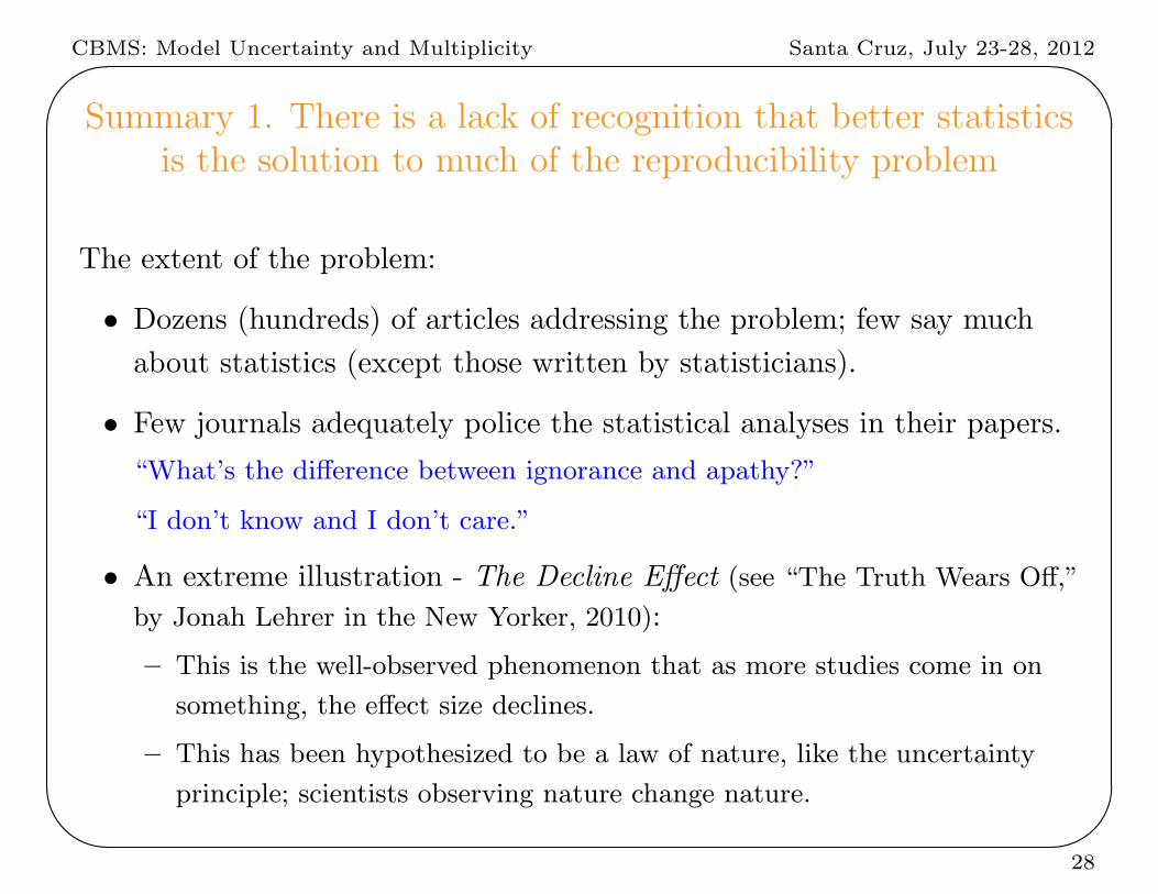
Summary 1. There is a lack of recognition that better statisticsis the solution to much of the reproducibility problem
The extent of the problem:
• Dozens (hundreds) of articles addressing the problem; few say much
about statistics (except those written by statisticians).
• Few journals adequately police the statistical analyses in their papers.
“What’s the difference between ignorance and apathy?”
“I don’t know and I don’t care.”
• An extreme illustration - The Decline Effect (see “The Truth Wears Off,”
by Jonah Lehrer in the New Yorker, 2010):
– This is the well-observed phenomenon that as more studies come in on
something, the effect size declines.
– This has been hypothesized to be a law of nature, like the uncertainty
principle; scientists observing nature change nature.
28
CBMS: Model Uncertainty and Multiplicity Santa Cruz, July 23-28, 2012'
&
$
%
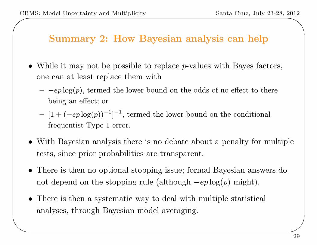
Summary 2: How Bayesian analysis can help
• While it may not be possible to replace p-values with Bayes factors,
one can at least replace them with
– −ep log(p), termed the lower bound on the odds of no effect to there
being an effect; or
– [1 + (−ep log(p))−1]−1, termed the lower bound on the conditional
frequentist Type 1 error.
• With Bayesian analysis there is no debate about a penalty for multiple
tests, since prior probabilities are transparent.
• There is then no optional stopping issue; formal Bayesian answers do
not depend on the stopping rule (although −ep log(p) might).
• There is then a systematic way to deal with multiple statistical
analyses, through Bayesian model averaging.
29
CBMS: Model Uncertainty and Multiplicity Santa Cruz, July 23-28, 2012'
&
$
%
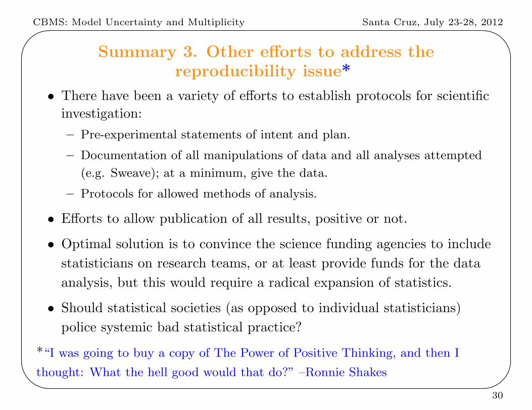
Summary 3. Other efforts to address thereproducibility issue*
• There have been a variety of efforts to establish protocols for scientific
investigation:
– Pre-experimental statements of intent and plan.
– Documentation of all manipulations of data and all analyses attempted
(e.g. Sweave); at a minimum, give the data.
– Protocols for allowed methods of analysis.
• Efforts to allow publication of all results, positive or not.
• Optimal solution is to convince the science funding agencies to include
statisticians on research teams, or at least provide funds for the data
analysis, but this would require a radical expansion of statistics.
• Should statistical societies (as opposed to individual statisticians)
police systemic bad statistical practice?
*“I was going to buy a copy of The Power of Positive Thinking, and then I
thought: What the hell good would that do?” –Ronnie Shakes
30

CBMS: Model Uncertainty and Multiplicity Santa Cruz, July 23-28, 2012'
&
$
%
II. A Brief History of (Objective) BayesianStatistics
31
CBMS: Model Uncertainty and Multiplicity Santa Cruz, July 23-28, 2012'
&
$
%
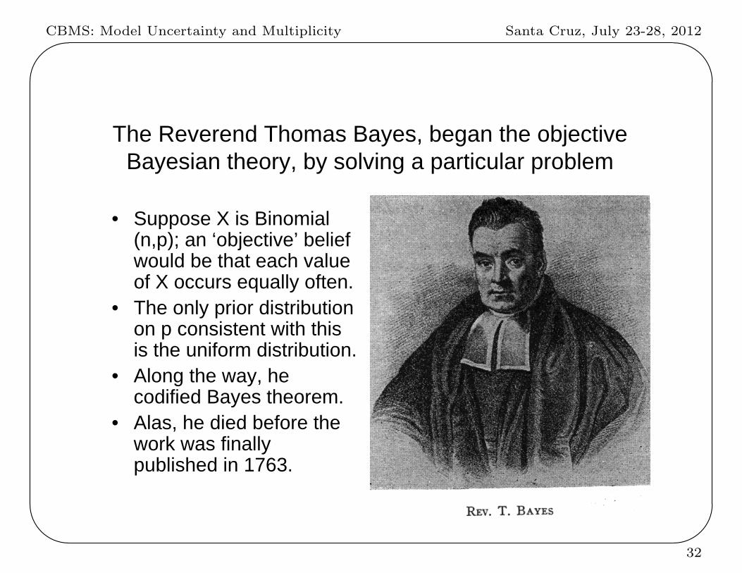
The Reverend Thomas Bayes, began the objectiveBayesian theory, by solving a particular problem
• Suppose X is Binomial(n,p); an ‘objective’ beliefwould be that each valueof X occurs equally often.
• The only prior distributionon p consistent with thisis the uniform distribution.
• Along the way, hecodified Bayes theorem.
• Alas, he died before thework was finallypublished in 1763.
32

CBMS: Model Uncertainty and Multiplicity Santa Cruz, July 23-28, 2012'
&
$
%
The real inventor of Objective Bayes was Simon Laplace(also a great mathematician, astronomer and civil servant)
who wrote Théorie Analytique des Probabilité in 1812
• He virtually always utilized a‘constant’ prior density (andclearly said why he did so).
• He established the ‘central limittheorem’ showing that, for largeamounts of data, the posteriordistribution is asymptoticallynormal (and the prior does notmatter).
• He solved very many applications,especially in physical sciences.
• He had numerous methodologicaldevelopments, e.g., a version ofthe Fisher exact test.
33
CBMS: Model Uncertainty and Multiplicity Santa Cruz, July 23-28, 2012'
&
$
%
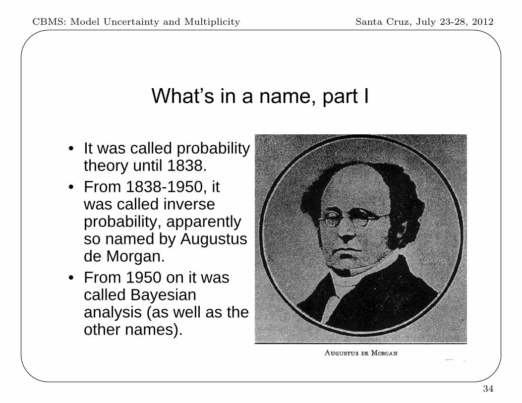
• It was called probabilitytheory until 1838.
• From 1838-1950, itwas called inverseprobability, apparentlyso named by Augustusde Morgan.
• From 1950 on it wascalled Bayesiananalysis (as well as theother names).
34

CBMS: Model Uncertainty and Multiplicity Santa Cruz, July 23-28, 2012'
&
$
%
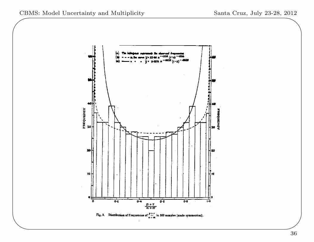
The importance of inverse probability b.f. (beforeFisher): as an example, Egon Pearson in 1925 finding
the ‘right’ objective prior for a binomial proportion
• Gathered a large number ofestimates of proportions pifrom different binomialexperiments
• Treated these as arising fromthe predictive distributioncorresponding to a fixed prior.
• Estimated the underlying priordistribution (an early empiricalBayes analysis).
• Recommended somethingclose to the currentlyrecommended ‘Jeffreys prior’p-1/2(1-p)-1/2.
35
CBMS: Model Uncertainty and Multiplicity Santa Cruz, July 23-28, 2012'
&
$
%36
CBMS: Model Uncertainty and Multiplicity Santa Cruz, July 23-28, 2012'
&
$
%
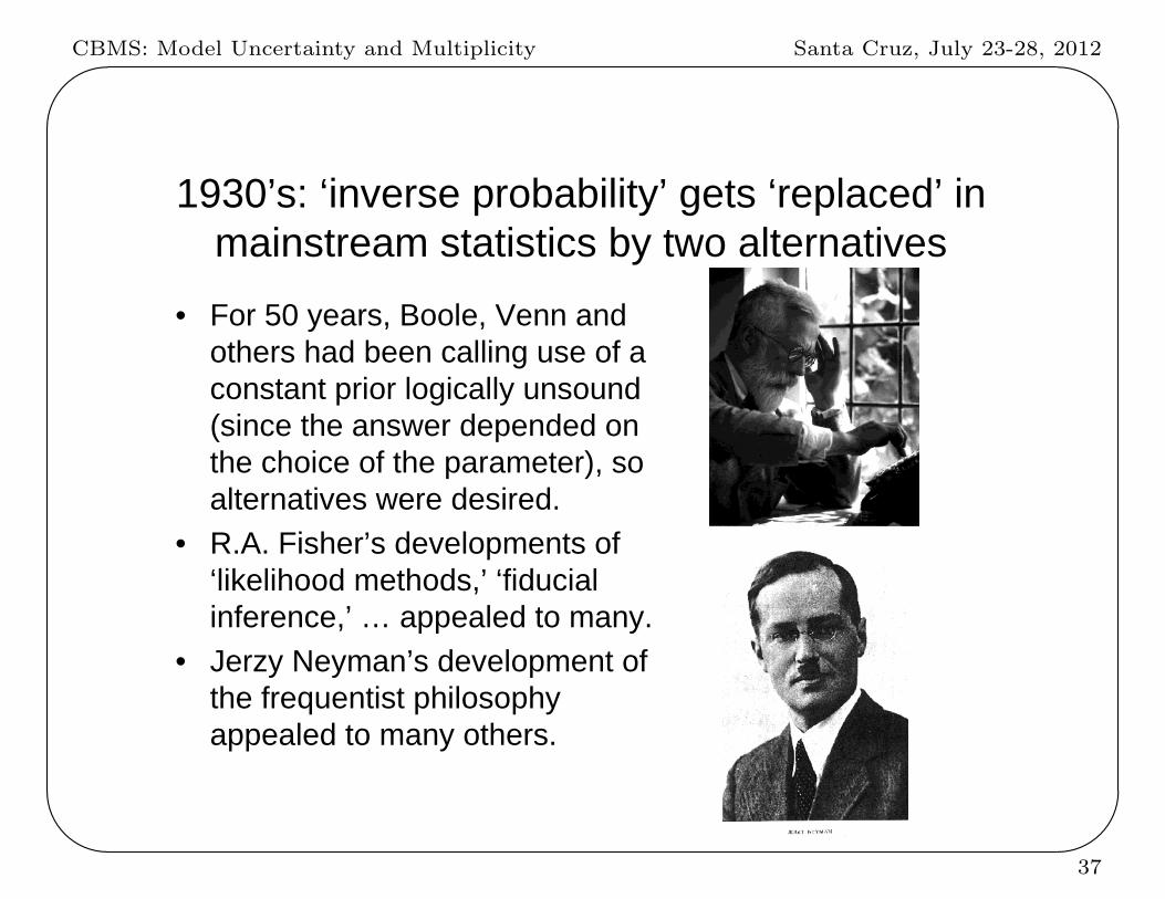
1930’s: ‘inverse probability’ gets ‘replaced’ inmainstream statistics by two alternatives
• For 50 years, Boole, Venn andothers had been calling use of aconstant prior logically unsound(since the answer depended onthe choice of the parameter), soalternatives were desired.
• R.A. Fisher’s developments of‘likelihood methods,’ ‘fiducialinference,’ … appealed to many.
• Jerzy Neyman’s development ofthe frequentist philosophyappealed to many others.
37
CBMS: Model Uncertainty and Multiplicity Santa Cruz, July 23-28, 2012'
&
$
%
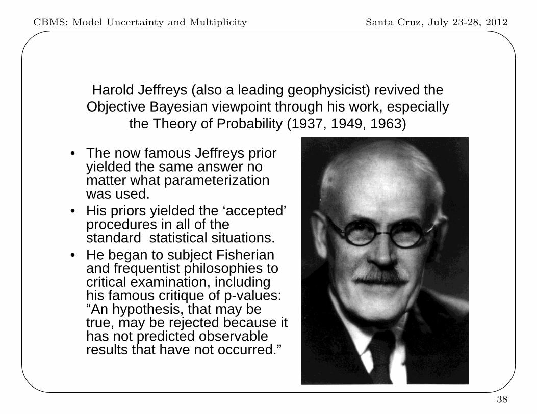
Harold Jeffreys (also a leading geophysicist) revived theObjective Bayesian viewpoint through his work, especially
the Theory of Probability (1937, 1949, 1963)
• The now famous Jeffreys prioryielded the same answer nomatter what parameterizationwas used.
• His priors yielded the ‘accepted’procedures in all of thestandard statistical situations.
• He began to subject Fisherianand frequentist philosophies tocritical examination, includinghis famous critique of p-values:“An hypothesis, that may betrue, may be rejected because ithas not predicted observableresults that have not occurred.”
38

CBMS: Model Uncertainty and Multiplicity Santa Cruz, July 23-28, 2012'
&
$
%
• In the 50’s and 60’s thesubjective Bayesian approachwas popularized (de Finetti,Rubin, Savage, Lindley, …)
• At the same time, the objectiveBayesian approach was beingrevived by Jeffreys, butBayesianism becameincorrectly associated with thesubjective viewpoint. Indeed,– only a small fraction of Bayesian
analyses done today heavilyutilize subjective priors;
– objective Bayesian methodologydominates entire fields ofapplication today.
39

CBMS: Model Uncertainty and Multiplicity Santa Cruz, July 23-28, 2012'
&
$
%
III. Could Fisher, Jeffreys and Neyman HaveAgreed on Testing?
40
CBMS: Model Uncertainty and Multiplicity Santa Cruz, July 23-28, 2012'
&
$
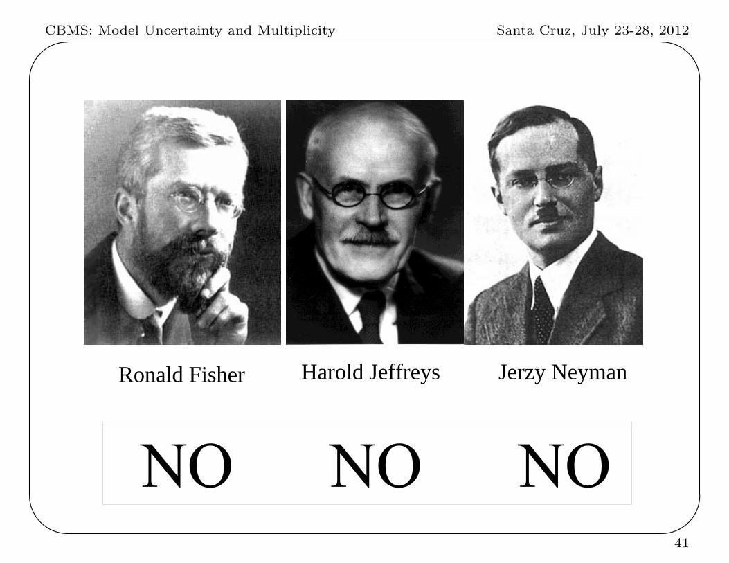
%Could they have agreed on testing methodology?
Ronald Fisher Harold Jeffreys Jerzy Neyman
41
CBMS: Model Uncertainty and Multiplicity Santa Cruz, July 23-28, 2012'
&
$
%
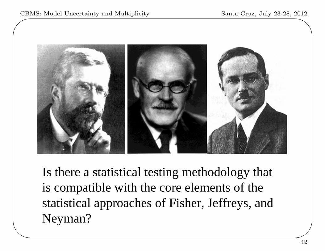
Is there a statistical testing methodology thatis compatible with the core elements of thestatistical approaches of Fisher, Jeffreys, andNeyman?
42

CBMS: Model Uncertainty and Multiplicity Santa Cruz, July 23-28, 2012'
&
$
%
Disagreements and Disagreements
• Fisher, Jeffreys and Neyman Disagreed as to the correct foundations of
statistics, but often agreed on the statistical procedure to use.
– All supported use of the same estimation and confidence procedures
for the normal linear model
– Disagreeing only on the interpretation (e.g., to be assigned to the
statement (x− 1.96 σ√n, x+ 1.96 σ√
n) is a 95% confidence interval for
a normal mean).
• In testing, however, they Disagreed as to the basic numbers to be
reported. Was this unavoidable?
43

CBMS: Model Uncertainty and Multiplicity Santa Cruz, July 23-28, 2012'
&
$
%44
CBMS: Model Uncertainty and Multiplicity Santa Cruz, July 23-28, 2012'
&
$
%45
CBMS: Model Uncertainty and Multiplicity Santa Cruz, July 23-28, 2012'
&
$
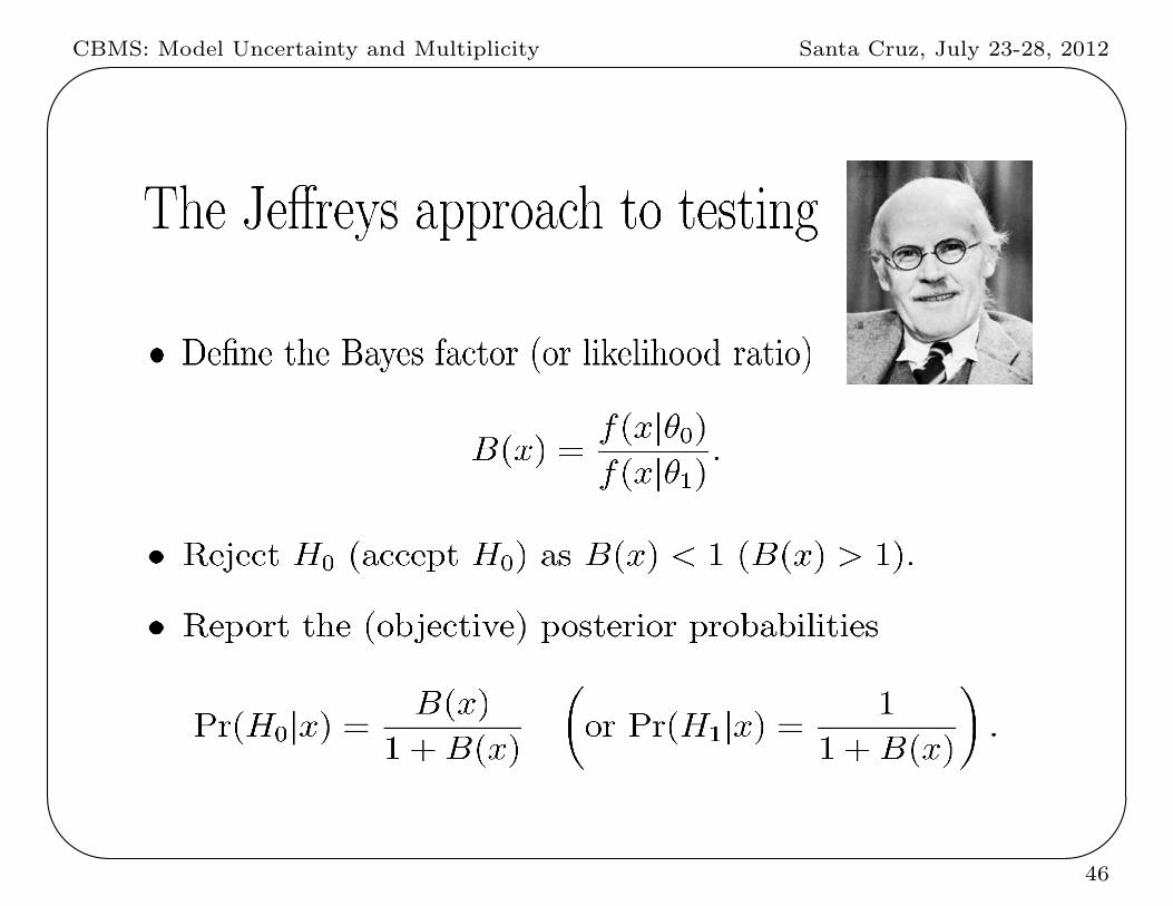
%46
CBMS: Model Uncertainty and Multiplicity Santa Cruz, July 23-28, 2012'
&
$
%
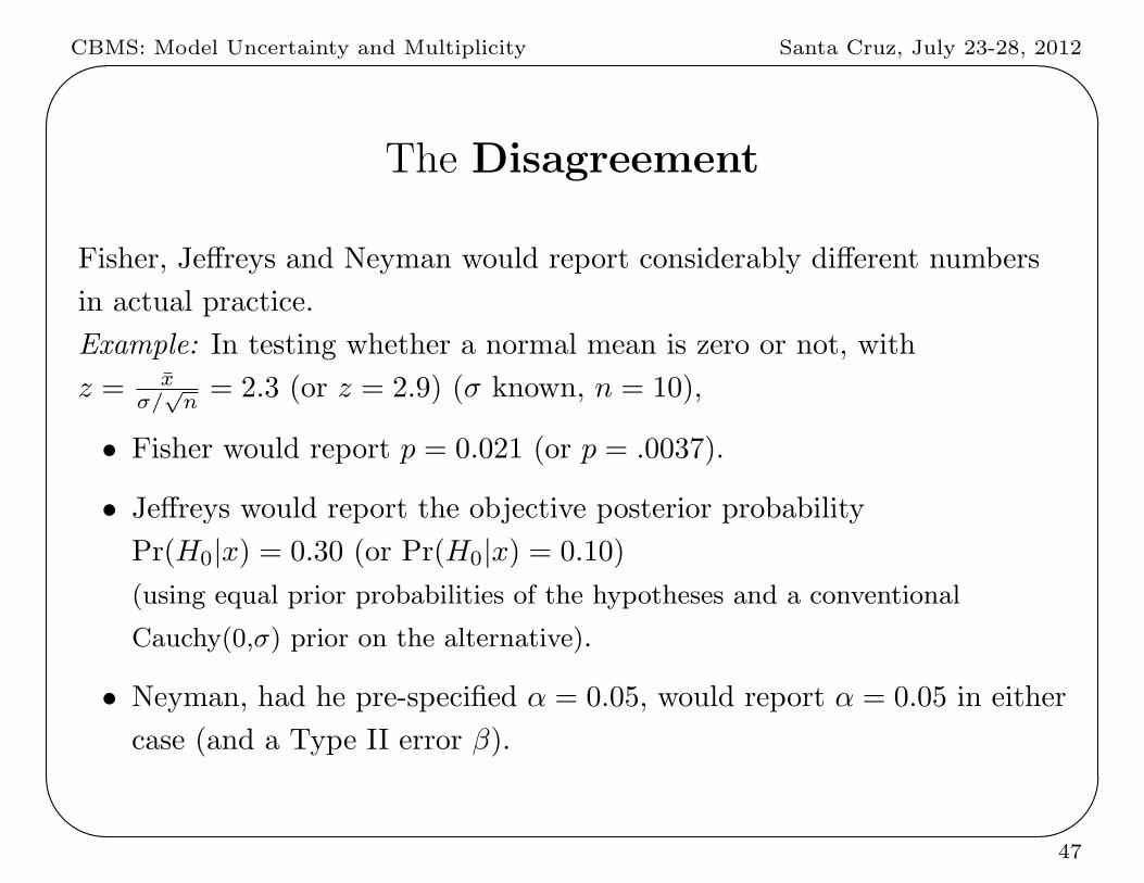
The Disagreement
Fisher, Jeffreys and Neyman would report considerably different numbers
in actual practice.
Example: In testing whether a normal mean is zero or not, with
z = xσ/
√n= 2.3 (or z = 2.9) (σ known, n = 10),
• Fisher would report p = 0.021 (or p = .0037).
• Jeffreys would report the objective posterior probability
Pr(H0|x) = 0.30 (or Pr(H0|x) = 0.10)
(using equal prior probabilities of the hypotheses and a conventional
Cauchy(0,σ) prior on the alternative).
• Neyman, had he pre-specified α = 0.05, would report α = 0.05 in either
case (and a Type II error β).
47

CBMS: Model Uncertainty and Multiplicity Santa Cruz, July 23-28, 2012'
&
$
%
Their criticisms of the other approaches
• Criticisms of Bayesian analysis in general. (Fisher and Neyman rarely
addressed Jeffreys particular version of Bayesian theory.)
– Fisher and Neyman rejected pre-Jeffreys objective Bayesian analysis
as logically flawed.
– Fisher’s subsequent position was that Bayesian analysis is based on
prior information that is only rarely available.
– Neyman, in addition, assumed that Bayesian analysis violated the
Frequentist Principle.
48
CBMS: Model Uncertainty and Multiplicity Santa Cruz, July 23-28, 2012'
&
$
%
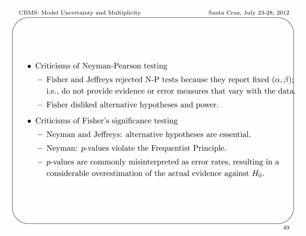
• Criticisms of Neyman-Pearson testing
– Fisher and Jeffreys rejected N-P tests because they report fixed (α, β);
i.e., do not provide evidence or error measures that vary with the data.
– Fisher disliked alternative hypotheses and power.
• Criticisms of Fisher’s significance testing
– Neyman and Jeffreys: alternative hypotheses are essential.
– Neyman: p-values violate the Frequentist Principle.
– p-values are commonly misinterpreted as error rates, resulting in a
considerable overestimation of the actual evidence against H0.
49

CBMS: Model Uncertainty and Multiplicity Santa Cruz, July 23-28, 2012'
&
$
%
One indication of the non-frequentist nature of p-values can be seen from
the applet (of German Molina) at
www.stat.duke.edu/∼berger
The situation considered follows Neyman’s proposals to evaluate testing
methods by simulations on a long series of different testing problems.
Suppose the ith test consists of
• normal data with unknown mean θi and known variance;
• testing of H0 : θi = 0 versus H1 : θi = 0.
The applet simulates a long series of such tests, and records how often H0
is true for p-values in given ranges.
50
CBMS: Model Uncertainty and Multiplicity Santa Cruz, July 23-28, 2012'
&
$
%
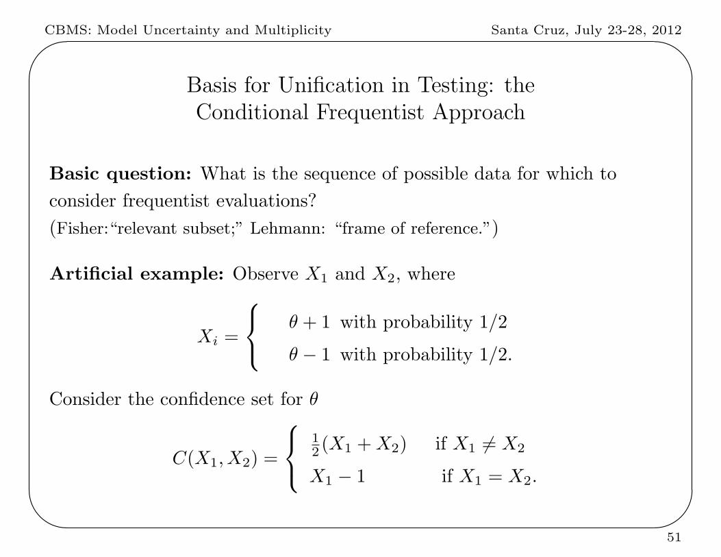
Basis for Unification in Testing: theConditional Frequentist Approach
Basic question: What is the sequence of possible data for which to
consider frequentist evaluations?
(Fisher:“relevant subset;” Lehmann: “frame of reference.”)
Artificial example: Observe X1 and X2, where
Xi =
θ + 1 with probability 1/2
θ − 1 with probability 1/2.
Consider the confidence set for θ
C(X1, X2) =
12 (X1 +X2) if X1 = X2
X1 − 1 if X1 = X2.
51
CBMS: Model Uncertainty and Multiplicity Santa Cruz, July 23-28, 2012'
&
$
%
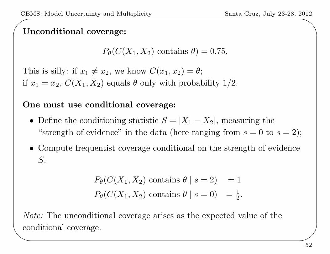
Unconditional coverage:
Pθ(C(X1, X2) contains θ) = 0.75.
This is silly: if x1 = x2, we know C(x1, x2) = θ;
if x1 = x2, C(X1, X2) equals θ only with probability 1/2.
One must use conditional coverage:
• Define the conditioning statistic S = |X1 −X2|, measuring the
“strength of evidence” in the data (here ranging from s = 0 to s = 2);
• Compute frequentist coverage conditional on the strength of evidence
S.
Pθ(C(X1, X2) contains θ | s = 2) = 1
Pθ(C(X1, X2) contains θ | s = 0) = 12 .
Note: The unconditional coverage arises as the expected value of the
conditional coverage.
52

CBMS: Model Uncertainty and Multiplicity Santa Cruz, July 23-28, 2012'
&
$
%
Conditional frequentist testing
• Find a statistic, S(x), whose magnitude indicates the “strength of
evidence” in x.
• Compute error probabilities as
α(s) = Type I error prob, given S(x) = s
= P0(Reject H0 | S(x) = s)
β(s) = Type II error prob, given S(x) = s
= P1(Accept H0 | S(x) = s)
53
CBMS: Model Uncertainty and Multiplicity Santa Cruz, July 23-28, 2012'
&
$
%
History of conditional frequentist testing
• Many Fisherian precursors based on conditioning on ancillary statistics
and on other statistics (e.g., the Fisher exact test, conditioning on
marginal totals).
• General theory in Kiefer (1977 JASA); the key step was in
understanding that almost any conditioning is formally allowed within
the frequentist paradigm (ancillarity is not required).
• Brown (1978) found optimal conditioning frequentist tests for
‘symmetric’, simple hypotheses.
• Berger, Brown and Wolpert (1994 AOS) developed the theory
discussed herein for testing simple hypotheses.
54
CBMS: Model Uncertainty and Multiplicity Santa Cruz, July 23-28, 2012'
&
$
%
Our suggested choice of the conditioning statistic
• Let pi be the p-value from testing Hi against the other hypothesis; use
the pi as measures of ‘strength of evidence,’ as Fisher suggested.
• Define the conditioning statistic S = maxp0, p1; its use is based on
deciding that data (in either the rejection or acceptance regions) with
the same p-value has the same ‘strength of evidence.’
55
CBMS: Model Uncertainty and Multiplicity Santa Cruz, July 23-28, 2012'
&
$
%
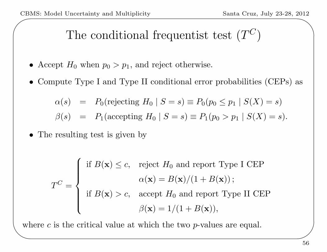
The conditional frequentist test (TC)
• Accept H0 when p0 > p1, and reject otherwise.
• Compute Type I and Type II conditional error probabilities (CEPs) as
α(s) = P0(rejecting H0 | S = s) ≡ P0(p0 ≤ p1 | S(X) = s)
β(s) = P1(accepting H0 | S = s) ≡ P1(p0 > p1 | S(X) = s).
• The resulting test is given by
TC =
if B(x) ≤ c, reject H0 and report Type I CEP
α(x) = B(x)/(1 +B(x)) ;
if B(x) > c, accept H0 and report Type II CEP
β(x) = 1/(1 +B(x)),
where c is the critical value at which the two p-values are equal.
56
CBMS: Model Uncertainty and Multiplicity Santa Cruz, July 23-28, 2012'
&
$
%
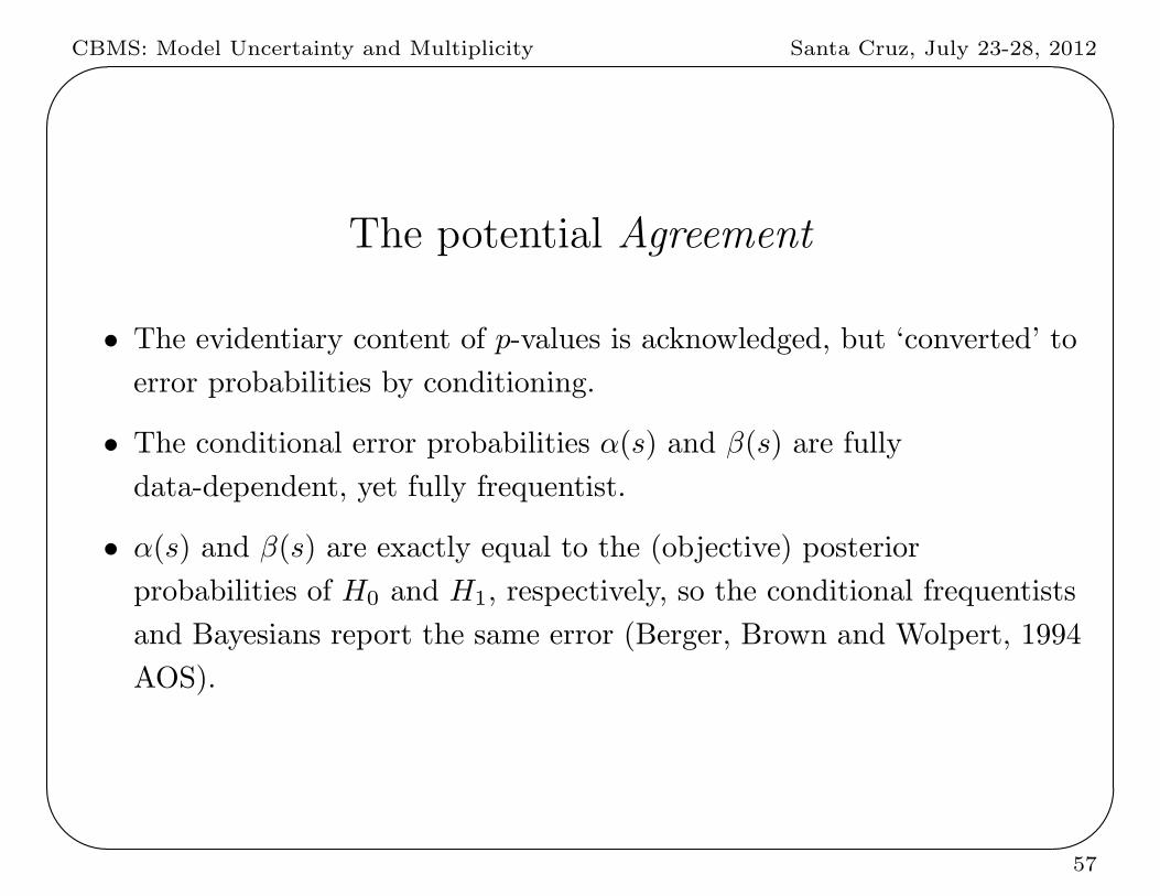
The potential Agreement
• The evidentiary content of p-values is acknowledged, but ‘converted’ to
error probabilities by conditioning.
• The conditional error probabilities α(s) and β(s) are fully
data-dependent, yet fully frequentist.
• α(s) and β(s) are exactly equal to the (objective) posterior
probabilities of H0 and H1, respectively, so the conditional frequentists
and Bayesians report the same error (Berger, Brown and Wolpert, 1994
AOS).
57
CBMS: Model Uncertainty and Multiplicity Santa Cruz, July 23-28, 2012'
&
$
%
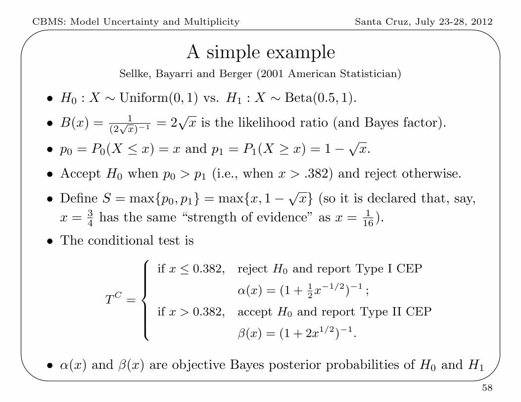
A simple exampleSellke, Bayarri and Berger (2001 American Statistician)
• H0 : X ∼ Uniform(0, 1) vs. H1 : X ∼ Beta(0.5, 1).
• B(x) = 1(2
√x)−1 = 2
√x is the likelihood ratio (and Bayes factor).
• p0 = P0(X ≤ x) = x and p1 = P1(X ≥ x) = 1−√x.
• Accept H0 when p0 > p1 (i.e., when x > .382) and reject otherwise.
• Define S = maxp0, p1 = maxx, 1−√x (so it is declared that, say,
x = 34 has the same “strength of evidence” as x = 1
16 ).
• The conditional test is
TC =
if x ≤ 0.382, reject H0 and report Type I CEP
α(x) = (1 + 12x−1/2)−1 ;
if x > 0.382, accept H0 and report Type II CEP
β(x) = (1 + 2x1/2)−1.
• α(x) and β(x) are objective Bayes posterior probabilities of H0 and H1
58
CBMS: Model Uncertainty and Multiplicity Santa Cruz, July 23-28, 2012'
&
$
%
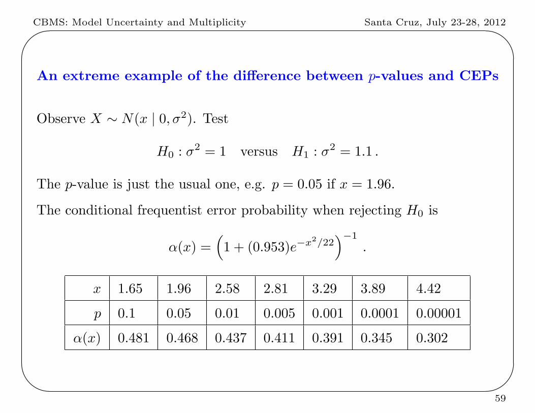
An extreme example of the difference between p-values and CEPs
Observe X ∼ N(x | 0, σ2). Test
H0 : σ2 = 1 versus H1 : σ2 = 1.1 .
The p-value is just the usual one, e.g. p = 0.05 if x = 1.96.
The conditional frequentist error probability when rejecting H0 is
α(x) =(1 + (0.953)e−x2/22
)−1
.
x 1.65 1.96 2.58 2.81 3.29 3.89 4.42
p 0.1 0.05 0.01 0.005 0.001 0.0001 0.00001
α(x) 0.481 0.468 0.437 0.411 0.391 0.345 0.302
59
CBMS: Model Uncertainty and Multiplicity Santa Cruz, July 23-28, 2012'
&
$
%
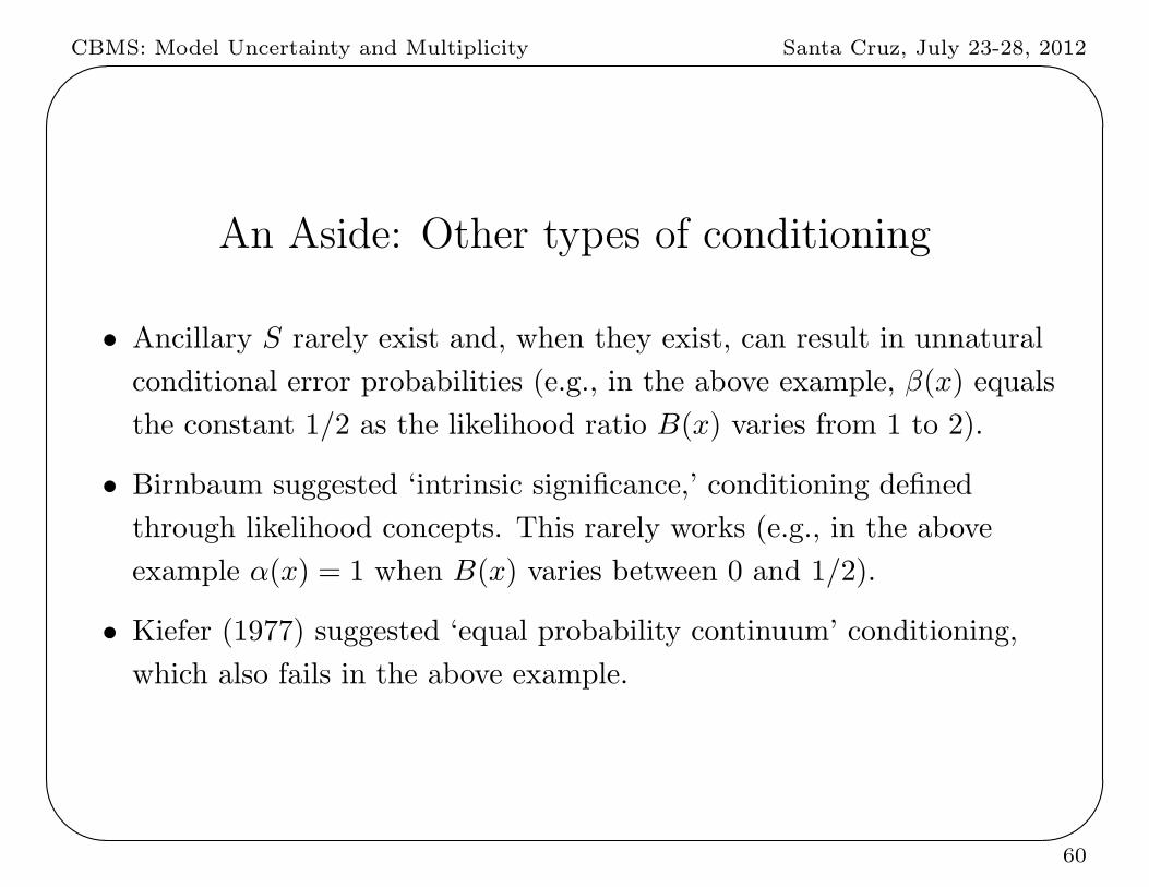
An Aside: Other types of conditioning
• Ancillary S rarely exist and, when they exist, can result in unnatural
conditional error probabilities (e.g., in the above example, β(x) equals
the constant 1/2 as the likelihood ratio B(x) varies from 1 to 2).
• Birnbaum suggested ‘intrinsic significance,’ conditioning defined
through likelihood concepts. This rarely works (e.g., in the above
example α(x) = 1 when B(x) varies between 0 and 1/2).
• Kiefer (1977) suggested ‘equal probability continuum’ conditioning,
which also fails in the above example.
60
CBMS: Model Uncertainty and Multiplicity Santa Cruz, July 23-28, 2012'
&
$
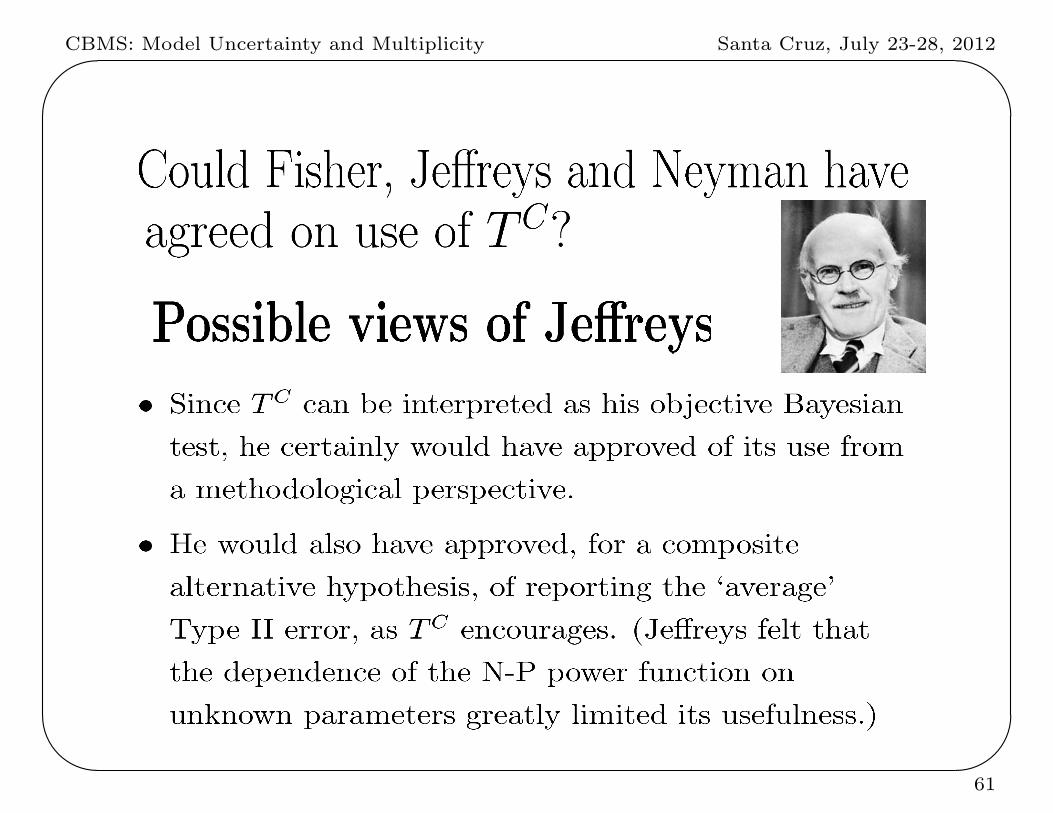
%61
CBMS: Model Uncertainty and Multiplicity Santa Cruz, July 23-28, 2012'
&
$
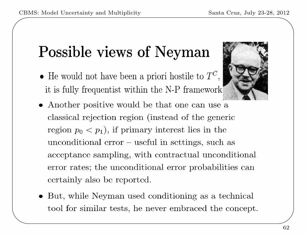
%62
CBMS: Model Uncertainty and Multiplicity Santa Cruz, July 23-28, 2012'
&
$
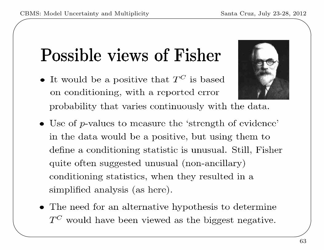
%63
CBMS: Model Uncertainty and Multiplicity Santa Cruz, July 23-28, 2012'
&
$
%
Generalizations of Conditional Frequentist Testing
• Berger, Boukai and Wang (1997a, 1997b) generalized to simple versus
composite hypothesis testing, including sequential settings.
• Dass (1998) generalized to discrete settings.
• Dass and Berger (2001) generalized to two composite hypotheses,
under partial invariance.
• Berger and Guglielmi (2001) used the ideas to create a finite sample
exact nonparametric test of fit.
64

CBMS: Model Uncertainty and Multiplicity Santa Cruz, July 23-28, 2012'
&
$
%
General Formulation (Dass and Berger, 2003 Scand. J. Stat.)
• Test H0 : X has density p0(x | η)versus H1 : X has density p1(x | η, ξon X , with respect to a σ-finite dominating measure λ.
• p0(x | η) : η ∈ Ω is invariant with respect to a group operation g ∈ G.
• g (η, ξ) = (g η, ξ) and p1(x | η, ξ) : η ∈ Ω is invariant with respect
to g for each given ξ.
• Utilize the right-haar prior, νG(η), on η and a proper prior π(ξ) on ξ.
• The original problem is reduced to testing distributions of the maximal
invariant, T:
H0 : T ∼ f0 versus H1 : T ∼ f1 ,
where f0(t) =∫p0(x | η)dνG(η) and f1(t) =
∫p1(x | η, ξ)dνG(η)dπ(ξ).
Since these are simple distributions, the rest of the analysis proceeds as
before, and the equivalence between posterior probabilities and
conditional frequentist error probabilities holds.
65
CBMS: Model Uncertainty and Multiplicity Santa Cruz, July 23-28, 2012'
&
$
%
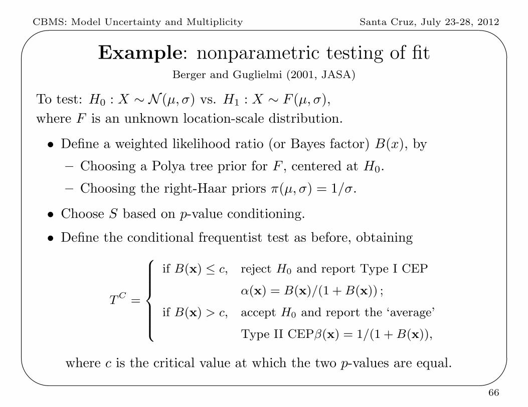
Example: nonparametric testing of fitBerger and Guglielmi (2001, JASA)
To test: H0 : X ∼ N (µ, σ) vs. H1 : X ∼ F (µ, σ),
where F is an unknown location-scale distribution.
• Define a weighted likelihood ratio (or Bayes factor) B(x), by
– Choosing a Polya tree prior for F , centered at H0.
– Choosing the right-Haar priors π(µ, σ) = 1/σ.
• Choose S based on p-value conditioning.
• Define the conditional frequentist test as before, obtaining
TC =
if B(x) ≤ c, reject H0 and report Type I CEP
α(x) = B(x)/(1 +B(x)) ;
if B(x) > c, accept H0 and report the ‘average’
Type II CEPβ(x) = 1/(1 +B(x)),
where c is the critical value at which the two p-values are equal.
66

CBMS: Model Uncertainty and Multiplicity Santa Cruz, July 23-28, 2012'
&
$
%
Notes:
• The Type I CEP again exactly equals the objective Bayesian posterior
probability of H0.
• The Type II CEP depends on (µ, σ). However, the ‘average’ Type II
CEP is the objective Bayesian posterior probability of H1.
• This gives exact conditional frequentist error probabilities, even for
small samples.
• Computation of B(x) uses the (simple) exact formula for a Polya tree
marginal distribution, together with importance sampling to deal with
(µ, σ).
67

CBMS: Model Uncertainty and Multiplicity Santa Cruz, July 23-28, 2012'
&
$
%
Other features of conditional frequentist testing withp-value conditioning
• Since the CEPs are also the objective Bayesian posterior probabilities
of the hypotheses,
– they do not depend on the stopping rule in sequential analysis, so
∗ their computation is much easier,
∗ one does not ‘spend α’ to look at the data;
– there is no danger of misinterpretation of a p-value as a frequentist
error probability, or misinterpretation of either as the posterior
probability that the hypothesis is true.
• One has exact frequentist tests for numerous situations where only
approximations were readily available before;
– computation of a CEP is easier than computation
of an unconditional error probability.
68
CBMS: Model Uncertainty and Multiplicity Santa Cruz, July 23-28, 2012'
&
$
%
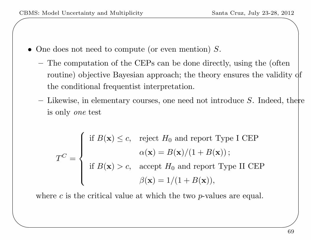
• One does not need to compute (or even mention) S.
– The computation of the CEPs can be done directly, using the (often
routine) objective Bayesian approach; the theory ensures the validity of
the conditional frequentist interpretation.
– Likewise, in elementary courses, one need not introduce S. Indeed, there
is only one test
TC =
if B(x) ≤ c, reject H0 and report Type I CEP
α(x) = B(x)/(1 +B(x)) ;
if B(x) > c, accept H0 and report Type II CEP
β(x) = 1/(1 +B(x)),
where c is the critical value at which the two p-values are equal.
69

CBMS: Model Uncertainty and Multiplicity Santa Cruz, July 23-28, 2012'
&
$
%
• For TC , the rejection and acceptance regions together span the entire
sample space, so that one might ‘reject’ and report CEP 0.40.
One could, instead:
– Specify an ordinary rejection region R (say, at the α = 0.05 level); note
that then α = E[α(s)1R].
– Find the ‘matching’ acceptance region, calling the region in the middle a
no decision region;
– Construct the corresponding conditional test.
– Note that the CEPs would not change.
70
CBMS: Model Uncertainty and Multiplicity Santa Cruz, July 23-28, 2012'
&
$
%
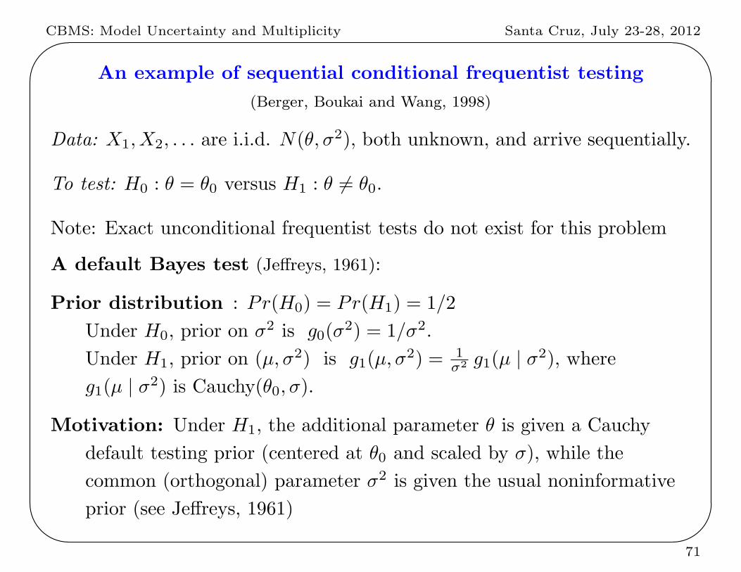
An example of sequential conditional frequentist testing
(Berger, Boukai and Wang, 1998)
Data: X1, X2, . . . are i.i.d. N(θ, σ2), both unknown, and arrive sequentially.
To test: H0 : θ = θ0 versus H1 : θ = θ0.
Note: Exact unconditional frequentist tests do not exist for this problem
A default Bayes test (Jeffreys, 1961):
Prior distribution : Pr(H0) = Pr(H1) = 1/2
Under H0, prior on σ2 is g0(σ2) = 1/σ2.
Under H1, prior on (µ, σ2) is g1(µ, σ2) = 1
σ2 g1(µ | σ2), where
g1(µ | σ2) is Cauchy(θ0, σ).
Motivation: Under H1, the additional parameter θ is given a Cauchy
default testing prior (centered at θ0 and scaled by σ), while the
common (orthogonal) parameter σ2 is given the usual noninformative
prior (see Jeffreys, 1961)
71
CBMS: Model Uncertainty and Multiplicity Santa Cruz, July 23-28, 2012'
&
$
%
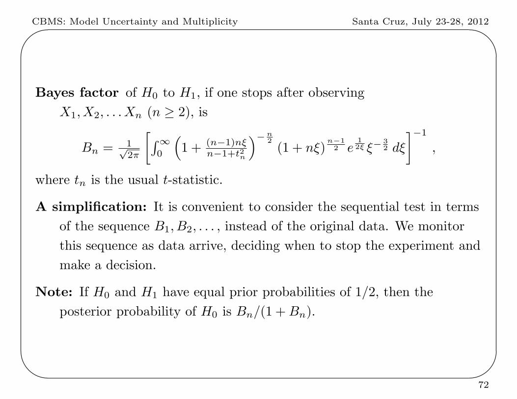
Bayes factor of H0 to H1, if one stops after observing
X1, X2, . . . Xn (n ≥ 2), is
Bn = 1√2π
[∫∞0
(1 + (n−1)nξ
n−1+t2n
)−n2
(1 + nξ)n−12 e
12ξ ξ−
32 dξ
]−1
,
where tn is the usual t-statistic.
A simplification: It is convenient to consider the sequential test in terms
of the sequence B1, B2, . . . , instead of the original data. We monitor
this sequence as data arrive, deciding when to stop the experiment and
make a decision.
Note: If H0 and H1 have equal prior probabilities of 1/2, then the
posterior probability of H0 is Bn/(1 +Bn).
72
CBMS: Model Uncertainty and Multiplicity Santa Cruz, July 23-28, 2012'
&
$
%
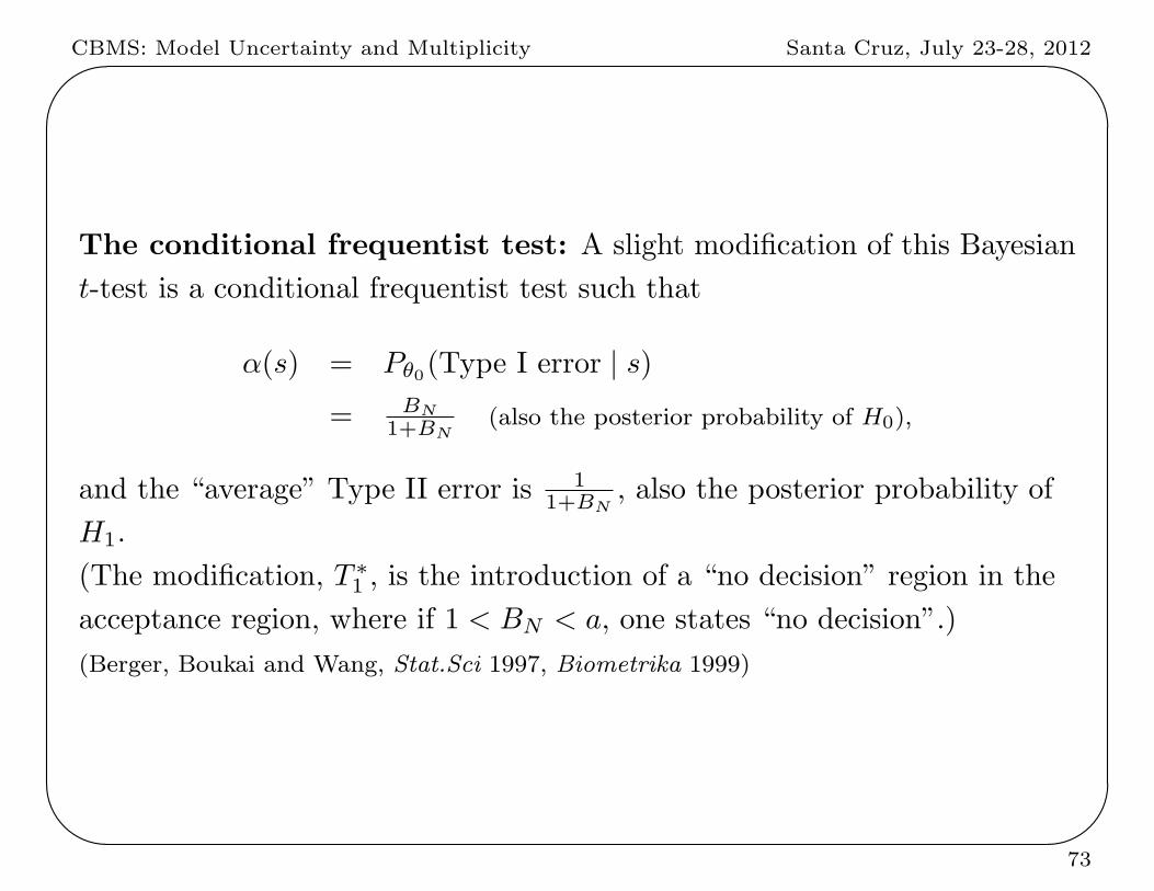
The conditional frequentist test: A slight modification of this Bayesian
t-test is a conditional frequentist test such that
α(s) = Pθ0(Type I error | s)
= BN
1+BN(also the posterior probability of H0),
and the “average” Type II error is 11+BN
, also the posterior probability of
H1.
(The modification, T ∗1 , is the introduction of a “no decision” region in the
acceptance region, where if 1 < BN < a, one states “no decision”.)
(Berger, Boukai and Wang, Stat.Sci 1997, Biometrika 1999)
73
CBMS: Model Uncertainty and Multiplicity Santa Cruz, July 23-28, 2012'
&
$
%
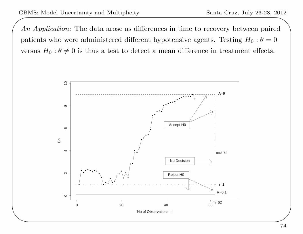
An Application: The data arose as differences in time to recovery between paired
patients who were administered different hypotensive agents. Testing H0 : θ = 0
versus H0 : θ = 0 is thus a test to detect a mean difference in treatment effects.
No of Observations n
Bn
0 20 40 60
02
46
810
•
••
• • • • • ••
•
• • ••
• ••
••
••
•
• •
• ••
• •• •
•
• •• • •
• • • • • • • • • • • • • ••
a=3.72
A=9
R=0.1
m=62
r=1
No Decision
Accept H0
Reject H0
74
CBMS: Model Uncertainty and Multiplicity Santa Cruz, July 23-28, 2012'
&
$
%
The stopping rule (any other could also be used):
If Bn ≤ R, Bn ≥ A or n = M , then stop the experiment.
Intuition:
R = “odds of H0 to H1” at which one would wish to stop and reject H0.
A = “odds of H0 to H1” at which one would wish to stop and accept H0.
M = maximum number of observations that can be taken
Example:
R = 0.1 (i.e., stop when 1 to 10 odds of H0 to H1)
A = 9 (i.e., stop when 9 to 1 odds of H0 to H1)
M = 62
75
CBMS: Model Uncertainty and Multiplicity Santa Cruz, July 23-28, 2012'
&
$
%
The test T ∗1 : If N denotes the stopping time,
T ∗1 =
if BN ≤ 1, reject H0 and report Type I CEP
α∗(BN ) = BN/(1 +BN ) ;
if 1 < BN < a, make no decision;
if BN ≥ a, accept H0 and report the ‘average’
Type II CEP β∗(BN ) = 1/(1 +BN ).
Example: a = 3.72 (found by simulation). For the actual data, the
stopping boundary would have been reached at time n = 52
(B52 = 9.017 > A = 9), and the conclusion would have been to accept
H0, and report error probability β∗(B52) = 1/(1 + 9.017) ≈ 0.100.
76
CBMS: Model Uncertainty and Multiplicity Santa Cruz, July 23-28, 2012'
&
$
%
Comments About the Sequential Test:
• T ∗1 is fully frequentist (and Bayesian).
• The conclusions and stopping boundary all have simple intuitive
interpretations.
• Computation is easy (except possibly computing a, but it is rarely
needed in practice):
– No stochastic process computations are needed.
– Computations do not change as the stopping rule changes.
– Sequential testing is as easy as fixed sample size testing.
• T ∗1 essentially follows the Stopping Rule Principle, which states that,
upon stopping experimentation, inference should not depend on the
reason experimentation stopped.
• This equivalence of conditional frequentist and Bayesian testing applies
to most classical testing scenarios.
77