AML 811Lecture 16

Case Study: Lid Driven Cavity Flow

Minor 2

Proposed date : Mar 27 (Fri) – Mar 30 (Mon).Please let me know now (latest by Friday) if this conflicts with any other Minors etc

Pattern : A few programs will be put up and you will be asked to make corrections, inferences, modifications etcWill also be split into basic, intermediate and advanced problems

Final Project

Default Project : Systematical computational analysis of boundary layer over a flat plateDue on Apr 28, last day of classAuditors

Those auditing the course officially need to either do a simple coding project or a literature review and answer a series of questions (your choice)Those auditing unofficially (just sitting in the class) obviously don’t need to do anything ☺

People taking the course for credit : Please stay back and a) Make a project group today and communicate it to me todayb) Choose on a project topic after discussing it with me today

Lid Driven Cavity flowFirst step of (all) incompressible NS based computational projects : An incompressible NS solver for Lid Driven Cavity flow

Staggered grid : x-momentum equation

The circled convective terms have to be found by interpolation as they don’t lie on the known grid points

This staggered grid formulation is also known as the Marker and Cell (MAC) formulation

Staggered grid : y-momentum equation

The circled convective terms have to be found by interpolation as they don’t lie on the known grid points

This staggered grid formulation is also known as the Marker and Cell (MAC) formulation

Now, we need to use the pressure Poisson equation to update the pressure

Discretizing the Pressure equation

Discretizing the Pressure equation

We need to use u, v at time level n for the RHS.

Discretization of the Pressure Poisson equation

The LHS is the usual 5-point finite difference for Poisson equationLeads to somewhat inaccurate transients because D is never really exactly zero.But, this method can be used for steady flows.

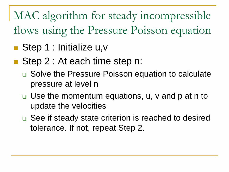
MAC algorithm for steady incompressible flows using the Pressure Poisson equation

Step 1 : Initialize u,vStep 2 : At each time step n:

Solve the Pressure Poisson equation to calculate pressure at level nUse the momentum equations, u, v and p at n to update the velocitiesSee if steady state criterion is reached to desired tolerance. If not, repeat Step 2.

A method for unsteady incompressible flows

The algorithm only satisfies the discretizedcontinuity equation approximatelyThere are also several other methods for steady incompressible flows. We’ll be discussing those when we deal with the finite volume methodFor an unsteady problem, we would like to ensure that the continuity equation is satisfied exactly (to machine precision) at each time step. There are several ways to do this. Let us try a small variation of the steady MAC method

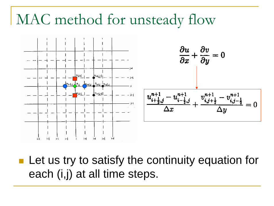
MAC method for unsteady flow

Let us try to satisfy the continuity equation for each (i,j) at all time steps.

MAC method for unsteady flow

Momentum equations

At each time step we can updatethe velocities using the momentumequations.However, we need to do this in a waywhich will satisfy continuity as well

MAC method for unsteady flow

Momentum equations

At each time step we can updatethe velocities using the momentumequations.However, we need to do this in a waywhich will satisfy continuity as well

The way to do this is to retain the above discretizations but change the pressure discretizations to time level n+1

MAC method for unsteady flow

Momentum equations

At each time step we can updatethe velocities using the momentumequations.However, we need to do this in a waywhich will satisfy continuity as well

The way to do this is to retain the above discretizations but change the pressure discretizations to time level n+1

( )

( )21,

1,

11,

1

21,

,21

1,

1,1

1

,21

+

+++

+

+

+

+++

+

+

+−∆∆

−=

+−∆∆

−=

ji

nji

nji

n

ji

ji

nji

nji

n

ji

RHSVppytv

RHSUppxtu

MAC for unsteady, incompressible flow

Initialize solution for velocity. This may or may not satisfy the discrete continuity equationAt each time step

1. Solve the pressure equation

⎥⎥⎥

⎦

⎤

⎢⎢⎢

⎣

⎡

∆

−+

∆

−

∆=

∆

+−+

∆

+−

−+−+

++

++−

++

++−

y

VHSRVHSR

x

HSURHSUR

t

yppp

xppp

jijijiji

nji

nji

nji

nji

nji

nji

21,

21,,

21,

21

2

11,

1,

11,

2

1,1

1,

1,1

1

22

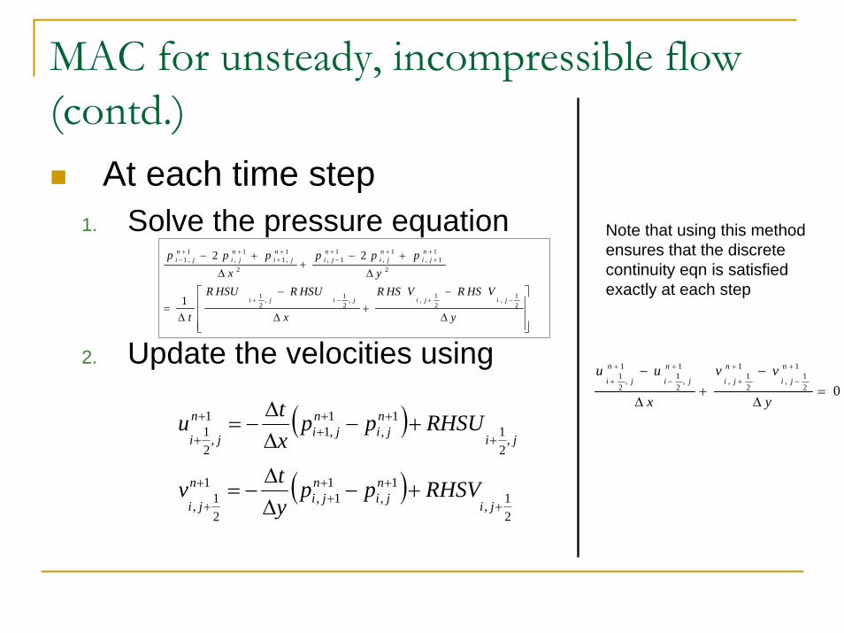
MAC for unsteady, incompressible flow (contd.)

At each time step 1. Solve the discrete Poisson equation

2. Update the velocities using⎥⎥⎥

⎦

⎤

⎢⎢⎢

⎣

⎡

∆

−+

∆

−

∆=

∆

+−+

∆

+−

−+−+

++

++−

++

++−

y

VHSRVHSR

x

HSURHSUR

t

yppp

xppp

jijijiji

nji

nji

nji

nji

nji

nji

21,

21,,

21,

21

2

11,

1,

11,

2

1,1

1,

1,1

1

22

( )

( )21,

1,

11,

1

21,

,21

1,

1,1

1

,21

+

+++

+

+

+

+++

+

+

+−∆∆

−=

+−∆∆

−=

ji

nji

nji

n

ji

ji

nji

nji

n

ji

RHSVppytv

RHSUppxtu

MAC for unsteady, incompressible flow (contd.)

At each time step 1. Solve the pressure equation

2. Update the velocities using⎥⎥⎥

⎦

⎤

⎢⎢⎢

⎣

⎡

∆

−+

∆

−

∆=

∆

+−+

∆

+−

−+−+

++

++−

++

++−

y

VHSRVHSR

x

HSURHSUR

t

yppp

xppp

jijijiji

nji

nji

nji

nji

nji

nji

21,

21,,

21,

21

2

11,

1,

11,

2

1,1

1,

1,1

1

22

( )

( )21,

1,

11,

1

21,

,21

1,

1,1

1

,21

+

+++

+

+

+

+++

+

+

+−∆∆

−=

+−∆∆

−=

ji

nji

nji

n

ji

ji

nji

nji

n

ji

RHSVppytv

RHSUppxtu

Note that using this methodensures that the discretecontinuity eqn is satisfiedexactly at each step

0

1

21,

1

21,

1

,21

1

,21

=∆

−+

∆

− +

−

+

+

+

−

+

+

y

vv

x

uu n

ji

n

ji

n

ji

n

ji

Summary of Lecture 15

MAC scheme for steady flows Explicit artificial compressibility method Pressure Poisson equation based method

MAC scheme for unsteady flowsDerive a Poisson equation after discretizing the flow equations This ensures that the discrete continuity equation is satisfied exactly

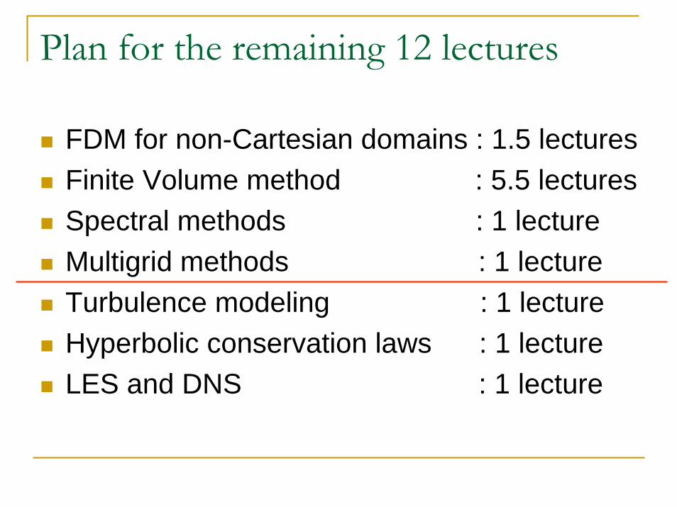
Plan for the remaining 12 lectures

FDM for non-Cartesian domains : 1.5 lecturesFinite Volume method : 5.5 lecturesSpectral methods : 1 lectureMultigrid methods : 1 lectureTurbulence modeling : 1 lectureHyperbolic conservation laws : 1 lectureLES and DNS : 1 lecture

Minor 2

Proposed date : Mar 27 (Fri) – Mar 30 (Mon).Please let me know now (latest by Friday) if this conflicts with any other Minors etc

Pattern : A few programs will be put up and you will be asked to make corrections, inferences, modifications etcWill also be split into basic, intermediate and advanced problems

Final Project

Default Project : Systematical computational analysis of boundary layer over a flat plateDue on Apr 28, last day of classAuditors

Those auditing the course officially need to either do a simple coding project or a literature review and answer a series of questions (your choice)Those auditing unofficially (just sitting in the class) obviously don’t need to do anything ☺

People taking the course for credit : Please stay back and a) Make a project group today and communicate it to me todayb) Choose on a project topic after discussing it with me today

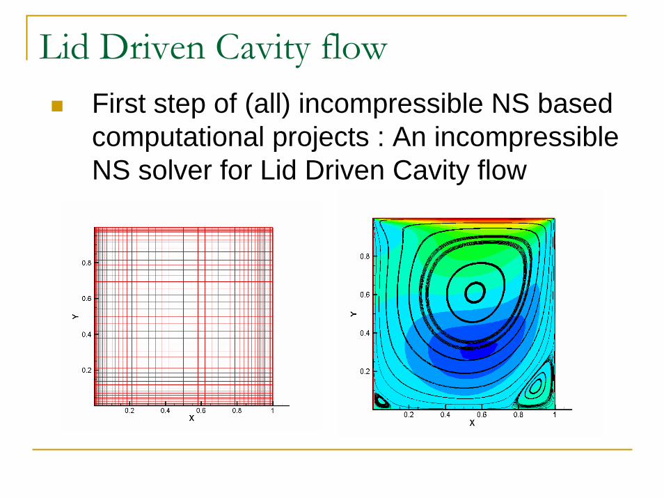
Lid Driven Cavity flowFirst step of (all) incompressible NS based computational projects : An incompressible NS solver for Lid Driven Cavity flow