lecture 2 overview of cge modeling - university of...

Lecture 2Overview of CGE Modeling

David Roland-Holst and Sam Heft-Neal, UC BerkeleyFaculty of EconomicsChiang Mai University

13 July 2010

Roland-Holst 2Chiang Mai University Faculty of Economics13 July 2010

GE Modeling Applications

1. SAM to CGE – A Very Basic Model2. The Thai_Mini Model3. Excel Implementation4. Scenario Examples


SAM Review

ACT COM VA HH GOV INV ROW TOTALS

ACT Gross Output

Receipts

COM Int. Use Household Consmption

GovernmentExpenditure

GrossInvestment

Exports Demand

VA GDP at Factor Cost

Factor Income

HH GDP at Factor Cost

ROW Trans. to HH

Household Income

GOV Net IndirectTaxes

Household Taxes

Government Borrowing

Government Revenue

INV Household Saving

Government Saving

Current account balance

Savings

ROW Imports ROW

TOTALS Payments Supply Factor Allocation

Household Expenditure

Government Expenditure

Investment ROW


SAM to CGE

• The SAM provides a snapshot of the economy at equilibrium (columns equal rows), but it is a static equilibrium with fixed prices, no substitution, and typically average behavior.

• On the contrary, in many cases what we are interested in examining is how economic actors respond to changes in relative prices.

• CGE allows for flexible prices, substitution, and marginal behavior, at the same time meeting the accounting constraints enforced by SAM structure.


SAM to CGE

• To put this another way, CGE models overcome the shortcomings of a SAM by specifying a functional form for every cell in the SAM.

• Each cell in the SAM can be represented by a price and quantity, so the model must be able to determine both prices and quantities.

• Let’s start with a VERY simple CGE model, then work our way to something a bit more complicated.


Very Basic CGE

• To see how we go from a SAM to a CGE model, let’s begin with a 2-sector, 2-factor really really simple SAM (RRSS):

Producers Factors Institutions ROWSUM

AG OTH L K HH

AG 150 150

OTH 500 500

L 100 200 150

K 50 300 150

HH 300 350 650

COLSUM 150 500 300 350 650


Our Simple Economy

• Note that the government is not an economic actor, the economy is closed, factor costs are the only input to production, and households spend all their income.

• In this case, we have three economic actors Producers (2; AG and OTH) Factors (2; L and K) Households (1)

• Let’s further assume that labor and capital are fully mobile across sectors (1 wage and rental rate).


Side Note

• (Let’s maintain our convention of having i be rows and j be columns; this means that i will reflect the income side of the economy and j will reflect the expenditure side of the economy).


Supply

• On the supply side, at a minimum we need to specify how producers behave (e.g., minimize costs), how they choose inputs (factor demands), and how their decisions determine aggregate supply. Using a Cobb-Douglas form, we can describe production within our economy as:

Total Supply

Labor Demand

Capital Demand


Demand

• On the demand side, we need to specify the level of household income, and how households decide to spend that income. Household income is the sum of factor incomes:

(Remember that we are decomposing SAM transactions into prices and, in this case, volumes.)


Demand

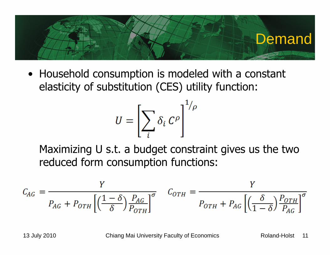
• Household consumption is modeled with a constant elasticity of substitution (CES) utility function:

Maximizing U s.t. a budget constraint gives us the two reduced form consumption functions:


Equilibrium

• Lastly, we need to define some sort of equilibrium conditions for the economy, which in our case we can represent by supply = demand in product and factor markets.

Commodity Market

Labor Market

Capital Market


Endogenous Variables

• In 13 equations we have built a simple general equilibrium model.

• Our 13 endogenous variables include: Pi – prices for AG and OTH goods r – rate of return on capital w – wage rate LDj – labor demand for AG and OTH producers KDj – capital demand for AG and OTH producers XSj – aggregate supply Ci – household consumption of AG and OTH goods Y – household income


Exogenous Variables

• We have left 2 variables exogenous: LS – Aggregate labor supply KS – Aggregate capital supply


Initializing Prices

• Prices are going to be endogenous in our simple CGE model, but we are going to represent prices in a price index rather than as absolute values. Prices can be initialized to any level, but 1 is generally the most obvious choice. PAG = 1 POTH = 1

• We select PAG as the numeraire, which fixes our economy-wide relative price as P = POTH / PAG


Initializing Prices

• We represent factor prices in the same way (as an index). w = 1 r = 1

(i.e., capital is more expensive in relative terms than labor)


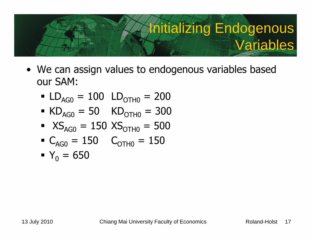
Initializing Endogenous Variables

• We can assign values to endogenous variables based our SAM: LDAG0 = 100 LDOTH0 = 200 KDAG0 = 50 KDOTH0 = 300 XSAG0 = 150 XSOTH0 = 500 CAG0 = 150 COTH0 = 150 Y0 = 650


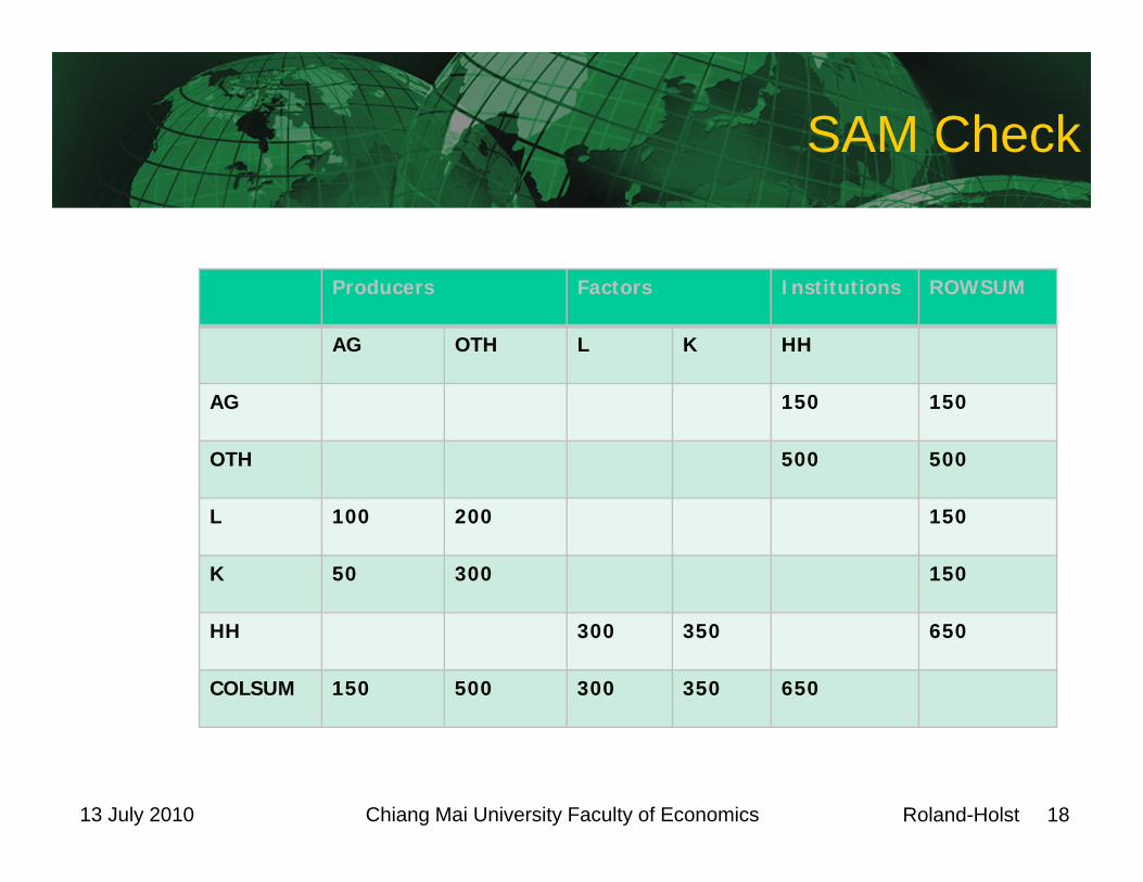
SAM Check

Producers Factors Institutions ROWSUM

AG OTH L K HH

AG 150 150

OTH 500 500

L 100 200 150

K 50 300 150

HH 300 350 650

COLSUM 150 500 300 350 650


Initializing Endogenous Variables

• LD, KD, XS, and C are volumes, so we need to convert them to volumes by dividing by the appropriate initialized price LDAG0/w0 = 100/1 =100 LDOTH0/w0 = 200/1 = 200 KDAG0/r0 = 50/1 = 50 KDOTH0/r0 = 300/1 = 300 XSAG0/pAG0 = 150/1 = 150 XSOTH0/pOTH0 = 500/1 =

500 CAG0/pAG0 = 150/1 = 150 COTH0/pOTH0 = 500/1

= 500

• We can also initialize LS and KS volumes LS0 = LDAG0+ LDOTH0 KS0 = KDAG0+ KDOTH0


Model Calibration

• We can use SAM data to determine the baseline values of some of our parameters; in this case: Cobb-Douglas scaling factors (Aj) Cobb-Douglas share parameters (αj) CES utility function share parameters (δ)


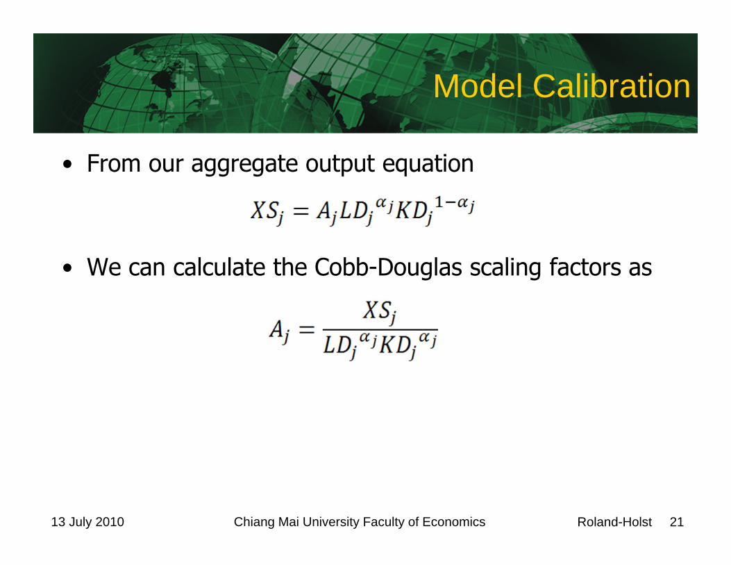
Model Calibration

• From our aggregate output equation

• We can calculate the Cobb-Douglas scaling factors as


Model Calibration

• Similarly, from labor demand

we can calculate the Cobb-Douglas share parameters as


Model Calibration

• The CES share parameters are derived from

with a less than tidy result of


Model Calibration

• Alternatively, the CES utility function’s substitution elasticity (σ) cannot be determined with SAM data.

• We can either specify σ heuristically (e.g., a 0 if we determine that the goods are perfect complements, or a high value if they are perfect substitutes) or through econometrics.

• In this case, let’s arbitrarily assign σ with a value of 0.3.


Model Simulation

• Let’s walk through what happens when we perturb one of the exogenous variables in the model. Say we have an exogenous increase in labor supply (LS). From

we know this exogenous increase in LS will be accompanied by an increase in aggregate LD.


Model Simulation

• But it isn’t clear how this change will affect our other variables:


To a New Equilibrium

• We need a way to move from our initial equilibrium, in which all of our model equations held (i.e., our markets cleared), to a new equilibrium, in which all of our equations hold again. This shift from an old equilibrium to a new equilibrium is what is usually meant by “adjustment.”

• To find our new equilibrium solution, our endogenous variables will have to adjust so that both our equations hold, and our exogenous shock is accounted for.


Model Solutions and Consistency

• CGE models require numerical solutions, which means that you will need to use some sort of solver package to generate a solution.

• To ensure that the model is consistent and you have not made errors in coding, in general your first step after building a CGE model is to make sure that you can reproduce the base solution (i.e., with no exogenous shock).


A Quick Thought on Model Building

• Before we get into more complex models, a bit of advice. It is always useful to start any research project with a quick theoretical model that maps relationships among the variables that you wish to examine.

• By doing this kind of exercise, you can get a good sense of where you can make simplifications, where you should be more detailed, and how much you can leave out of your model, and what your data requirements will be.


Toward more Complex Models

Our next model — THAI_MINI — is significantly more complex, but still simple as far as CGE models go.

THAIMINI will address several of the oversimplifications of our previous model: Producers typically have non-factor intermediate

inputs and non-uniform substitution elasticities Households are more complex than CES utility

describes Most economies have an active government and

capital markets Most economies have ROW interactions


Production - CES Stratification

= 0

m k

v

p XP

ND VA

L KF

K F

XAp

XM XDd

XP - OutputND - Aggregate intermediate demandVA - Value added bundleL - Demand for laborKF - Capital/sector specific capital bundleK - Demand for capitalF - Demand for sector specific factorXAp - Input/output matrixXDd - Domestic demand for domestic goodsXM - Demand for importssp -Top level substitution elasticity (ND and VA)sv -Substitution elasticity between L and KFsk -Substitution elasticity between K and Fsm - Armington elasticity


Production - CES Stratification

= 0

m k

v

p XP

ND VA

L KF

K F

XAp

XM XDd

XP - OutputND - Aggregate intermediate demandVA - Value added bundleL - Demand for laborKF - Capital/sector specific capital bundleK - Demand for capitalF - Demand for sector specific factorXAp – Aggregate (Dom+Imp) IntermediateXDd - Domestic demand for domestic goodsXM - Demand for importsp - Top level substitution elasticity(ND and VA) v - Substitution elasticity between L and KF k - Substitution elasticity between K and F m - Armington elasticity


Unit Costs and Prices(1)

(2)

(1) ii

indii XP

PNDPXND

pi

(2) ii

ivaii XP

PVAPXVA

pi

(3) pip

ipi

ivaii

ndii PVAPNDPX

1/111

(4) ipii PVAPP 1


Factor Demand I

(5) iil

ili

di VA

WPVAL

viv

i

1

(6) ii

ikfii VA

PKFPXKF

vi

(7)

vi

vi

vi

ikfil

i

lii PKFWPVA

1/1

11


Factor Demand II

(8) ii

iki

ki

di KF

RPKFK

ki

ki

1

(9) ii

ifi

fi

di KF

PFPKFF

ki

ki

1

(10)

kik

iki

fi

ifik

i

ikii

PFRPKF

1/111


Leontief Intermediate Technology

(11) jijij NDaXAp

(12) i

iitpijijj PAaPND 1


Household Income and Final Demand

(13) gh

i

dii

dii

di TRPFPFKRWLYH .

(14) DeprYYHYD 1

(15) iitci

iii PA

YXAc

1

*

(16) j

jjitcj PAYDY 1*

(17) i

iiitci

h XAcPAYDS 1

(18) 0.DeprYPDeprY


Government

(19) 0XGXG

(20) XGPA

PGXAgg

iitgi

gii

1

(21) g

g

ii

itgi

gi PAPG

1/1

11


Investment

(22) DeprYSERSSXIPI fgh ..

(23) XIPA

PIXAii

iitii

iii

1

(24) i

i

ii

itii

ii PAPI

1/1

11


Trade: Demand

(25) iiij

iji XAiXAgXAcXApXA

(26) ii

idi

di XA

PDPAXD

mi

(27) ii

imii XA

PMPAXM

mi

(28) mim

imi

imii

dii PMPDPA

1/111


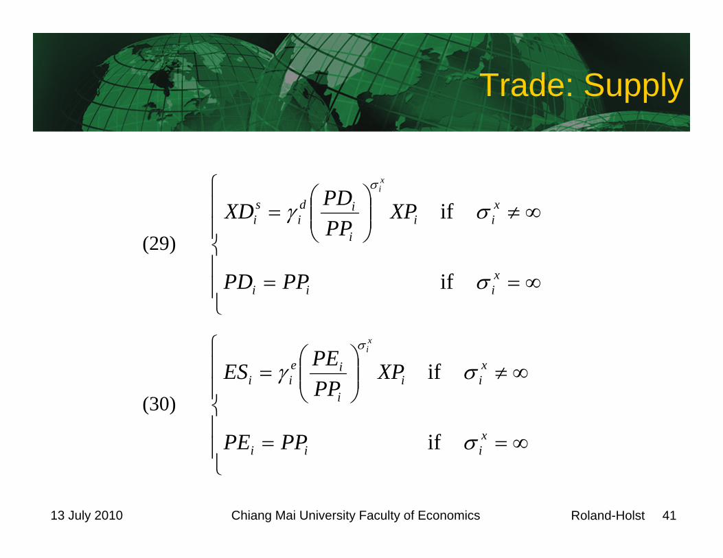
Trade: Supply

(29)

xiii

xii

i

idi

si

PPPD

XPPPPDXD

xi

if

if

(30)

xiii

xii

i

ieii

PPPE

XPPPPEES

xi

if

if


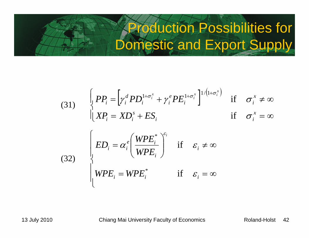
Production Possibilities for Domestic and Export Supply

(31)

xii

sii

xii

eii

dii

ESXDXP

PEPDPPxix

ixi

if

if1/111

(32)

iii

ii

ieii

WPEWPE

WPEWPEED

i

if

if

*

*


Trade Prices

(33) imii WPMERPM 1

(34) eiii WPEERPE 1/.


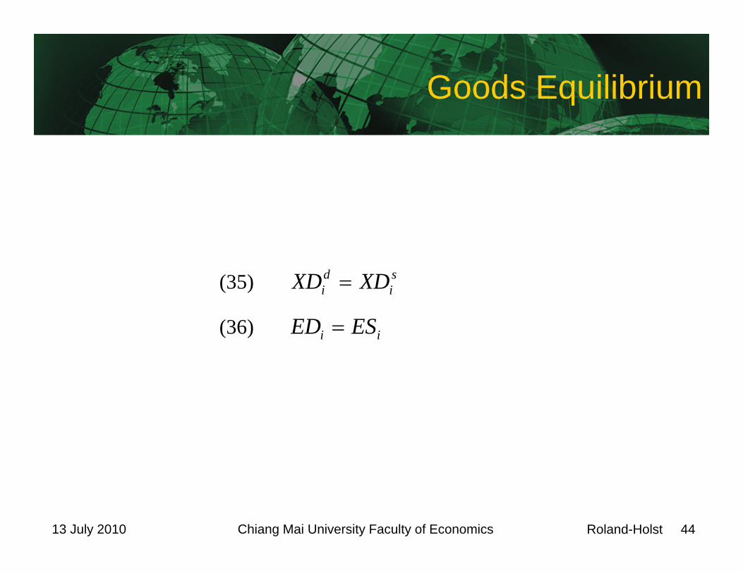
Goods Equilibrium

(35) si

di XDXD

(36) ii ESED


Factor Equilibrium

(37) l

PWL ls

(38) i

di

s LL


Capital Market Equilibrium

(39) ss TKTK 0

(40)

ki

ksiki

si

TRR

TKTRRK

k

if

if

(41)

k

i

di

s

k

ii

ki

KTK

RTRk

k

if

if1/1

1

(42) si

di KK


Other Resource Equilibrium

(43) f

i

PPFF if

is

i

(44) si

di FF


Macro Closure I: Fiscal

(45)

ii

itiii

itgii

itci

jij

itpiji XAiXAgXAcXApPAITaxY

(46) i

iiei

iii

mi ESPEXMWPMERTradeY

(47) YHXPPXTradeYITaxYGRevi

iipi .


Macro Closure II: Financial

(48) hg

g TRPXGPGGRevS ..

(49) PSRS gg /

(50) gg RSRS 0


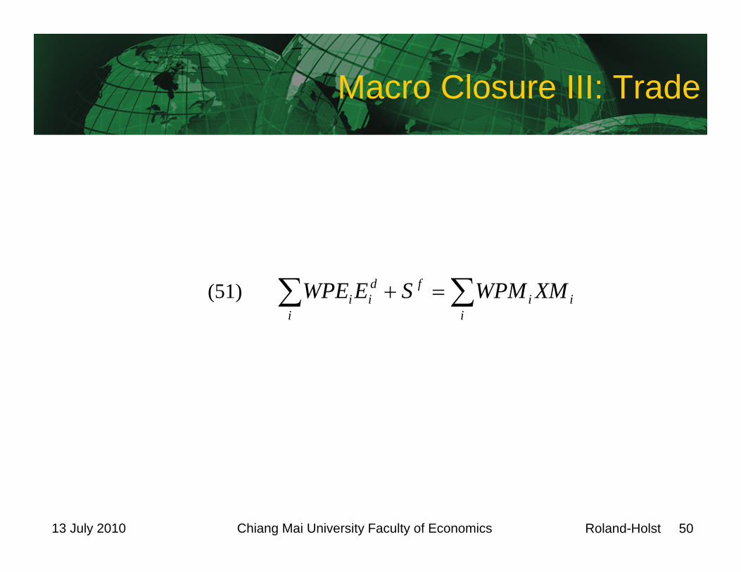
Macro Closure III: Trade

(51) i

iif

i

dii XMWPMSEWPE


Macro Closure IV: Numeraire

(52) i

dii

dii

di FPFKRWLGDPFC

(53) i

di

fii

di

kii

di

li FPFKRLWRGDP 0,0,0

(54) RGDPGDPFCP /


Excel Implementation for Thailand

Download the Excel spreadsheet Thai_Mini_CGE.xlsThis is a heuristic, 2 sector CGE model in six spreadsheets:1. AggMat – A matrix of zeros and ones to aggregate a

standard GTAP SAM to fit the two sector framework2. BaseSAM – The initial input SAM, taken from GTAP 5.3. SAM – The aggregated initial SAM and a counterfactual

SAM for comparative static assessment4. Model – The primary data and equation spreadsheet5. Parameters – A registry of structural parameter values6. Dictionary – complete definitions of variables and

parameters


Model Spreadsheet

This is the primary functional component of the Mini_CGE, containing all

1. Endogenous variables, 87 (suffixes _a and _o for agriculture and other)

2. Equations 86 (one is redundant because of WalrasLaw)

3. Exogenous variables, 27 and 4. A few examples of counterfactual experiments.


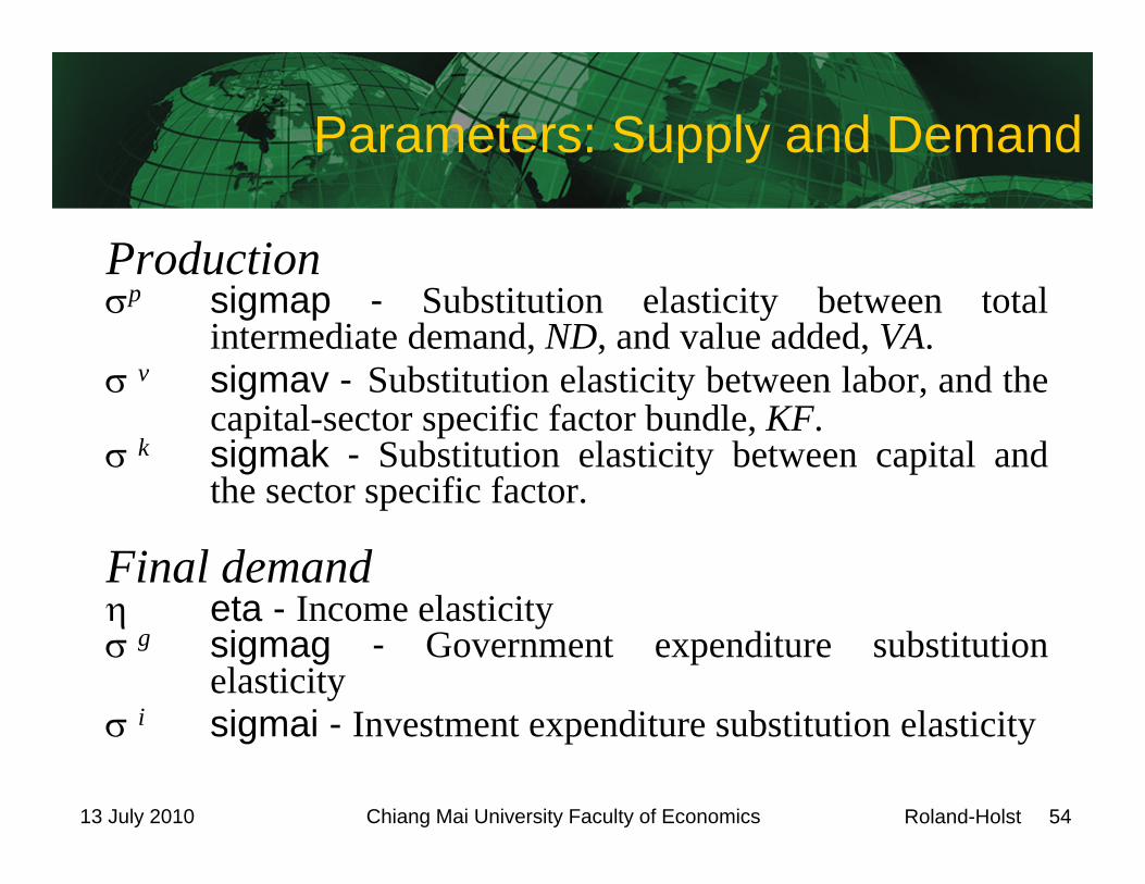
Parameters: Supply and Demand

Productionp sigmap - Substitution elasticity between total

intermediate demand, ND, and value added, VA. v sigmav - Substitution elasticity between labor, and the

capital-sector specific factor bundle, KF. k sigmak - Substitution elasticity between capital and

the sector specific factor.

Final demand eta - Income elasticity g sigmag - Government expenditure substitution

elasticity i sigmai - Investment expenditure substitution elasticity


Parameters – Trade and Factors

Trade elasticitiesm sigmam - Armington import elasticity x sigmax - CET transformation elasticity (between

domestic and export supply). epse - Export demand elasticity.

Supply elasticities l omegal - Aggregate labor supply elasticity k omegak - Capital mobility elasticity. 0 emulates sector-

specific capital. Use a high value to approximate perfectly mobile capital.

f sigmak - Sector-specific supply elasticities.


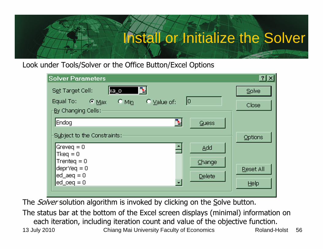
Install or Initialize the Solver

Look under Tools/Solver or the Office Button/Excel Options

The Solver solution algorithm is invoked by clicking on the Solve button. The status bar at the bottom of the Excel screen displays (minimal) information on

each iteration, including iteration count and value of the objective function.


Simulation Results

If successful, the solver will display the following dialog box:

To have the Solver overwrite the values of the endogenous variables, simply click on the OK button. Users can experiment with the other options.


Convergence and Consistency

If solution convergence was achieved, the model should have re-produced the base data set (within the limits of the convergence tolerance). All equations should evaluate to 0. The expression of Walras’ Law should evaluate to 0. All deviations from initial values should evaluate to 0. A final test is to check the consistency of the resulting SAM.

The SAM spreadsheet, contains the solution SAM. The solution SAM is expressed in terms of the model solution. For example, the labor remuneration cell (in agriculture) contains the formula:=wage*ld_a/scale

If the SAM is not consistent, either the solution is inconsistent, the model has been mis-specified, or the formulas in the SAM have been mis-specified. The formula is adjusted by the scale variable to make the solution SAM comparable with the initial SAM.


Homogeneity Test

If this is a new model, it is recommended to check model homogeneity. This involves a perturbation of the model numéraire. If the model is homogeneous in prices, perturbation of the model numéraire should leave all volumes constant, and adjust all prices and value variables by the same percentage amount as the percentage change in the numéraire(i.e. all relative prices remain constant). To check homogeneity, multiply the initial value of the numéraire by some constant, e.g. in cell L23, for the exchange rate substitute=er0*1.1

Initially, the only equations which will be affected by this change are the domestic investment equation, the domestic trade prices, and the tariff revenue equation because these are the only equations where the numéraire (the exchange rate) appears. Invoke Solver to find a new solution to the model. If the homogeneity test fails (other than due to the lack of convergence), at least one of the equations has been mis-specified, or there could be a built-in nominal rigidity, such as a fixed nominal wage. If both tests succeed, the model should be re-initialized, and the next step is to run one or more shocks to the model.


Installed Scenarios

1. Tariff Abolition2. Full Trade Reform3. Agricultural Export Tax4. Agricultural Export Price Changes5. Other Export Price Changes


Questions?

lecture 2 overview of cge modeling - university of...

Documents