lecture 3. experiments with a single factor: anovaminzhang/514_fall2016/lec...

Statistics 514: Experiments with One Single Factors: ANOVA Fall 2016

Lecture 3. Experiments with a Single Factor: ANOVA

Montgomery Sections 3.1 through 3.5 and Section 15.1.1

1 Lecture 3 –


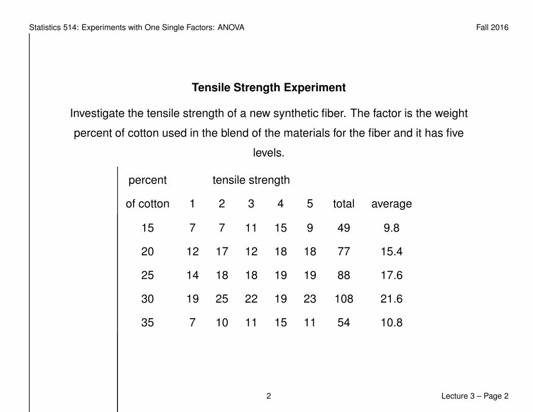
Tensile Strength Experiment

Investigate the tensile strength of a new synthetic fiber. The factor is the weight

percent of cotton used in the blend of the materials for the fiber and it has five

levels.

percent tensile strength

of cotton 1 2 3 4 5 total average

15 7 7 11 15 9 49 9.8

20 12 17 12 18 18 77 15.4

25 14 18 18 19 19 88 17.6

30 19 25 22 19 23 108 21.6

35 7 10 11 15 11 54 10.8

2 Lecture 3 –


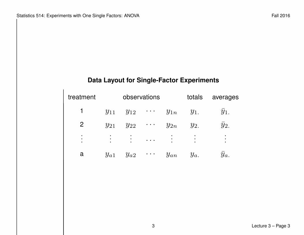
Data Layout for Single-Factor Experiments

treatment observations totals averages

1 y11 y12 · · · y1n y1. y1.

2 y21 y22 · · · y2n y2. y2....

.

.

.... · · ·

.

.

....

.

.

.

a ya1 ya2 · · · yan ya. ya.

3 Lecture 3 –


Analysis of Variance

• Statistical Model (Factor Effects Model):

yij = µ+ τi + ǫij

i = 1, 2 . . . , a

j = 1, 2, . . . , ni

µ - grand mean; τi - ith treatment effect; ǫijiid∼ N(0, σ2) - error

Constraint:∑a

i=1 τi = 0 (Conceptual Approach; SAS: τa = 0).

• Estimates for parameters:

µ = y..

τi = (yi. − y..)

ǫij = yij − yi. ( residual )

• Basic Hypotheses:

H0 : τ1 = τ2 = . . . = τa = 0 vs H1 : τi 6= 0 for at least one i

4 Lecture 3 –


Analysis of Variance (ANOVA) Table

Source of Sum of Degrees of Mean F0

Variation Squares Freedom Square

Between SSTreatment a− 1 MSTreatment F0

Within SSE N − a MSE

Total SST N − 1

• If balanced: N = n× a

SST =∑∑

y2ij − y2../N ; SSTreatment =1n

∑

y2i. − y2../N

SSE=SST - SSTreatment

• If unbalanced: N =∑a

i=1 ni

SST =∑∑

y2ij − y2../N ; SSTreatment =∑ y2

i.

ni− y2../N

SSE=SST - SSTreatment

• SSTreatments =∑a

i=1 niτ2i and SSE =

∑

i

∑

j ǫ2ij .

5 Lecture 3 –


• The Expected Mean Squares (EMS) are

E(MSE)=σ2

E(MSTreatment) = σ2 +∑

niτ2i /(a− 1)

• Test Statistic

F0 =SSTreatments/(a− 1)

SSE/(N − a)=

MSTreatments

MSE

• Under H0:

F0 =SSTreatment/σ

2(a− 1)

SSE/σ2(N − a)=

χ2a−1/(a− 1)

χ2N−a/(N − a)

∼ Fa−1,N−a

• Decision Rule: If F0 > Fα,a−1,N−a then reject H0

• When a = 2, the square of the t-test statistic t20 = MSTreatment

MSE

= F0.

– F -test and two-sample two-sided test are equivalent.

6 Lecture 3 –


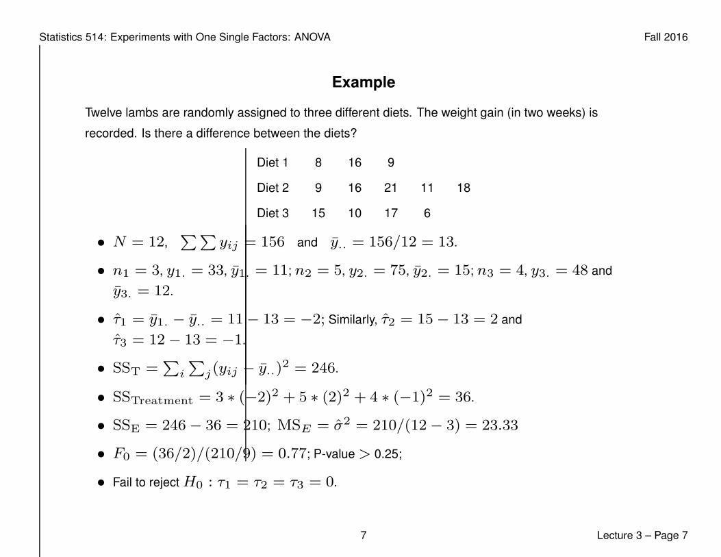
Example

Twelve lambs are randomly assigned to three different diets. The weight gain (in two weeks) is

recorded. Is there a difference between the diets?

Diet 1 8 16 9

Diet 2 9 16 21 11 18

Diet 3 15 10 17 6

• N = 12,∑∑

yij = 156 and y.. = 156/12 = 13.

• n1 = 3, y1. = 33, y1. = 11; n2 = 5, y2. = 75, y2. = 15; n3 = 4, y3. = 48 and

y3. = 12.

• τ1 = y1. − y.. = 11− 13 = −2; Similarly, τ2 = 15− 13 = 2 and

τ3 = 12− 13 = −1.

• SST =∑

i

∑j(yij − y..)2 = 246.

• SSTreatment = 3 ∗ (−2)2 + 5 ∗ (2)2 + 4 ∗ (−1)2 = 36.

• SSE = 246− 36 = 210; MSE = σ2 = 210/(12− 3) = 23.33

• F0 = (36/2)/(210/9) = 0.77; P-value > 0.25;

• Fail to reject H0 : τ1 = τ2 = τ3 = 0.

7 Lecture 3 –


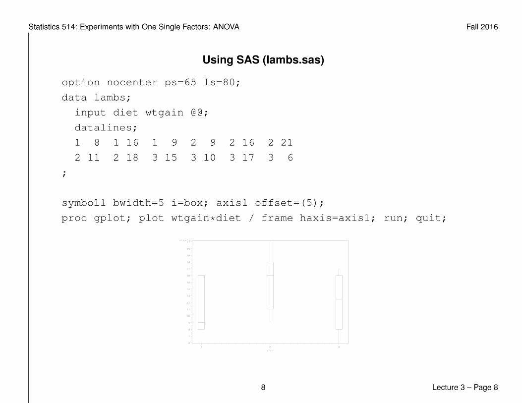
Using SAS (lambs.sas)

option nocenter ps=65 ls=80;

data lambs;

input diet wtgain @@;

datalines;

1 8 1 16 1 9 2 9 2 16 2 21

2 11 2 18 3 15 3 10 3 17 3 6

;

symbol1 bwidth=5 i=box; axis1 offset=(5);

proc gplot; plot wtgain*diet / frame haxis=axis1; run; quit;

8 Lecture 3 –


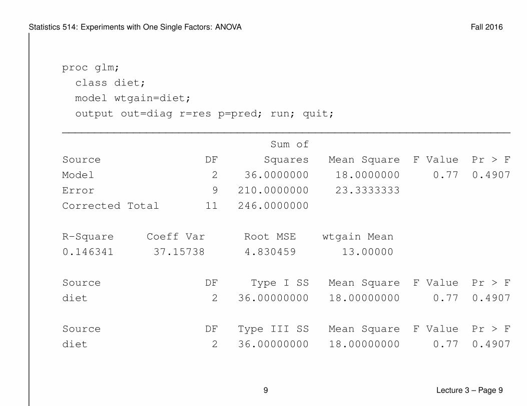
proc glm;

class diet;

model wtgain=diet;

output out=diag r=res p=pred; run; quit;

_____________________________________________________________________

Sum of

Source DF Squares Mean Square F Value Pr > F

Model 2 36.0000000 18.0000000 0.77 0.4907

Error 9 210.0000000 23.3333333

Corrected Total 11 246.0000000

R-Square Coeff Var Root MSE wtgain Mean

0.146341 37.15738 4.830459 13.00000

Source DF Type I SS Mean Square F Value Pr > F

diet 2 36.00000000 18.00000000 0.77 0.4907

Source DF Type III SS Mean Square F Value Pr > F

diet 2 36.00000000 18.00000000 0.77 0.4907

9 Lecture 3 –


proc gplot; plot res*diet /frame haxis=axis1;

proc sort; by pred;

symbol1 v=circle i=sm50;

proc gplot; plot res*pred / haxis=axis1;

run; quit;

10 Lecture 3 –


Model Checking and Diagnostics

• Model Assumptions

1 Model is correct

2 Independent observations

3 Errors normally distributed

4 Constant variance

yij = (y.. + (yi. − y..)) + (yij − yi.)

yij = yij + ǫij

observed = predicted + residual

• Note that the predicted response at treatment i is yij = yi.

• Diagnostics use predicted responses and residuals.

11 Lecture 3 –


Diagnostics

• Normality

– Histogram of residuals

– Normal probability plot / QQ plot

– Shapiro-Wilk Test

• Constant Variance

– Plot ǫij vs yij (residual plot)

– Bartlett’s or Modified Levene’s Test

• Independence

– Plot ǫij vs time/space

– Plot ǫij vs variable of interest

• Outliers

12 Lecture 3 –


Diagnostics Example: Tensile Strength Experiment

options ls=80 ps=60 nocenter;

goptions device=win target=winprtm rotate=landscape ftext=swiss

hsize=8.0in vsize=6.0in htext=1.5 htitle=1.5 hpos=60 vpos=60

horigin=0.5in vorigin=0.5in;

data one;

infile ’c:\saswork\data\tensile.dat’;

input percent strength time;

title1 ’Tensile Strength Example’;

proc print data=one; run;

_____________________________________________________________________

Obs percent strength time

1 15 7 15

2 15 7 19

3 15 15 25

4 15 11 12

5 15 9 6

6 20 12 8

: : : :

24 35 15 16

25 35 11 23

13 Lecture 3 –


symbol1 v=circle i=none;

title1 ’Plot of Strength vs Percent Blend’;

proc gplot data=one; plot strength*percent/frame; run;

proc boxplot;

plot strength*percent/boxstyle=skeletal pctldef=4; run;

14 Lecture 3 –


proc glm data=one;

class percent; model strength=percent;

means percent / hovtest=bartlett hovtest=levene;

output out=diag p=pred r=res; run;

____________________________________________________________________

Sum of

Source DF Squares Mean Square F Value Pr > F

Model 4 475.7600000 118.9400000 14.76 <.0001

Error 20 161.2000000 8.0600000


Levene’s Test for Homogeneity of strength Variance

ANOVA of Squared Deviations from Group Means

Sum of Mean

Source DF Squares Square F Value Pr > F

percent 4 91.6224 22.9056 0.45 0.7704

Error 20 1015.4 50.7720

Bartlett’s Test for Homogeneity of strength Variance

Source DF Chi-Square Pr > ChiSq

percent 4 0.9331 0.9198

15 Lecture 3 –


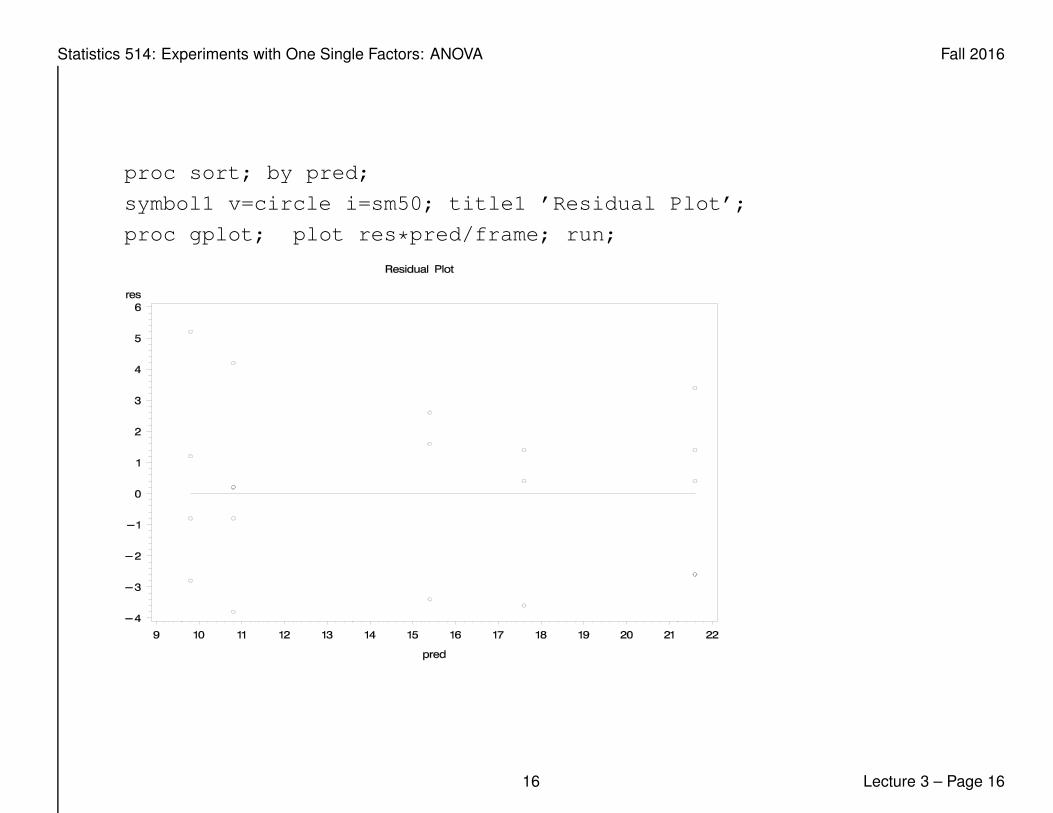
proc sort; by pred;

symbol1 v=circle i=sm50; title1 ’Residual Plot’;

proc gplot; plot res*pred/frame; run;

16 Lecture 3 –


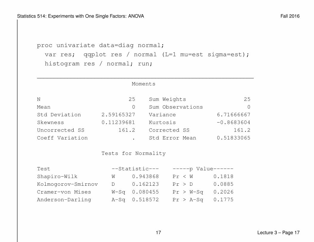
proc univariate data=diag normal;

var res; qqplot res / normal (L=1 mu=est sigma=est);

histogram res / normal; run;

________________________________________________________________

Moments

N 25 Sum Weights 25

Mean 0 Sum Observations 0

Std Deviation 2.59165327 Variance 6.71666667

Skewness 0.11239681 Kurtosis -0.8683604

Uncorrected SS 161.2 Corrected SS 161.2

Coeff Variation . Std Error Mean 0.51833065

Tests for Normality

Test --Statistic--- -----p Value------

Shapiro-Wilk W 0.943868 Pr < W 0.1818

Kolmogorov-Smirnov D 0.162123 Pr > D 0.0885

Cramer-von Mises W-Sq 0.080455 Pr > W-Sq 0.2026

Anderson-Darling A-Sq 0.518572 Pr > A-Sq 0.1775

17 Lecture 3 –


Histogram of Residuals & QQ Plot

18 Lecture 3 –


/* Time Serial Plot */

symbol1 v=circle i=none;

title1 ’Plot of residuals vs time’;

proc gplot; plot res*time / vref=0 vaxis=-6 to 6 by 1;

run;

19 Lecture 3 –


Non-Constant Variance: Impact and Remedy

• Does not affect F-test dramatically when the experiment is balanced

• Why concern?

– Comparison of treatments depends on MSE

– Incorrect intervals and comparison results

• Variance-Stabilizing Transformations

– Ideas for Finding Proper Transformations (E[Y ] = µ, Var(Y ) = σ2)

f(Y ) ≈ f(µ) + (Y − µ)f ′(µ)

=⇒ Var(f(Y )) ≈ [f ′(µ)]2Var(Y ) = [f ′(µ)]2σ2

∗ Find f such that Var(f(Y )) does not depend on µ anymore. So,

Y = f(Y ) has constant variance for different f(µ).

– Common transformations√x, log(x), 1/x, arcsin(

√x), and 1/

√x

20 Lecture 3 –


Transformations

• Suppose σ2 is a function of µ, that is σ2 = g(µ)

• Want to find transformation f such that Y = f(Y ) has constant variance:

Var(Y ) does not depend on µ.

• Have shown Var(Y )≈ [f ′(µ)]2σ2 ≈ [f ′(µ)]2g(µ)

• Want to choose f such that [f ′(µ)]2g(µ) ≈ c

Examples

g(µ) = µ (Poisson) f(µ) =∫

1√µdµ → f(X) =

√X

g(µ) = µ(1− µ) (Binomial) f(µ) =∫

1√µ(1−µ)

dµ → f(X) = arcsin(√X)

g(µ) = µ2β (Box-Cox) f(µ) =∫

µ−βdµ → f(X) = X1−β

g(µ) = µ2 (Box-Cox) f(µ) =∫

1µdµ → f(X) = logX

21 Lecture 3 –


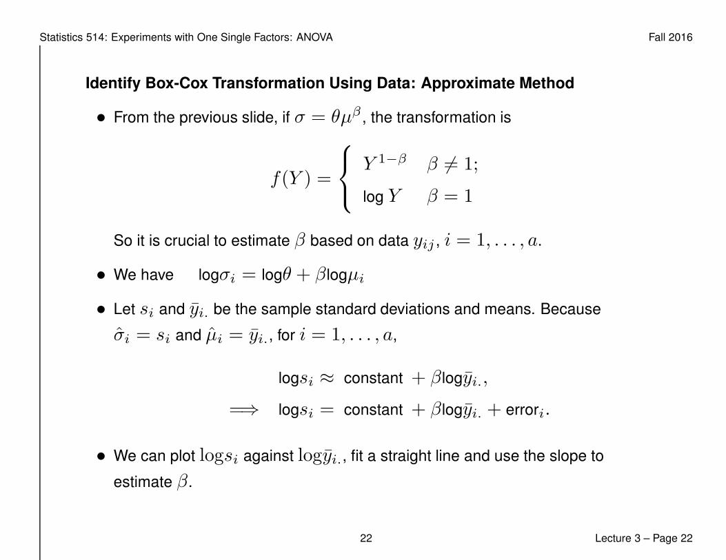
Identify Box-Cox Transformation Using Data: Approximate Method

• From the previous slide, if σ = θµβ , the transformation is

f(Y ) =

Y 1−β β 6= 1;

log Y β = 1

So it is crucial to estimate β based on data yij , i = 1, . . . , a.

• We have logσi = logθ + βlogµi

• Let si and yi. be the sample standard deviations and means. Because

σi = si and µi = yi., for i = 1, . . . , a,

logsi ≈ constant + βlogyi.,

=⇒ logsi = constant + βlogyi. + errori.

• We can plot logsi against logyi., fit a straight line and use the slope to

estimate β.

22 Lecture 3 –


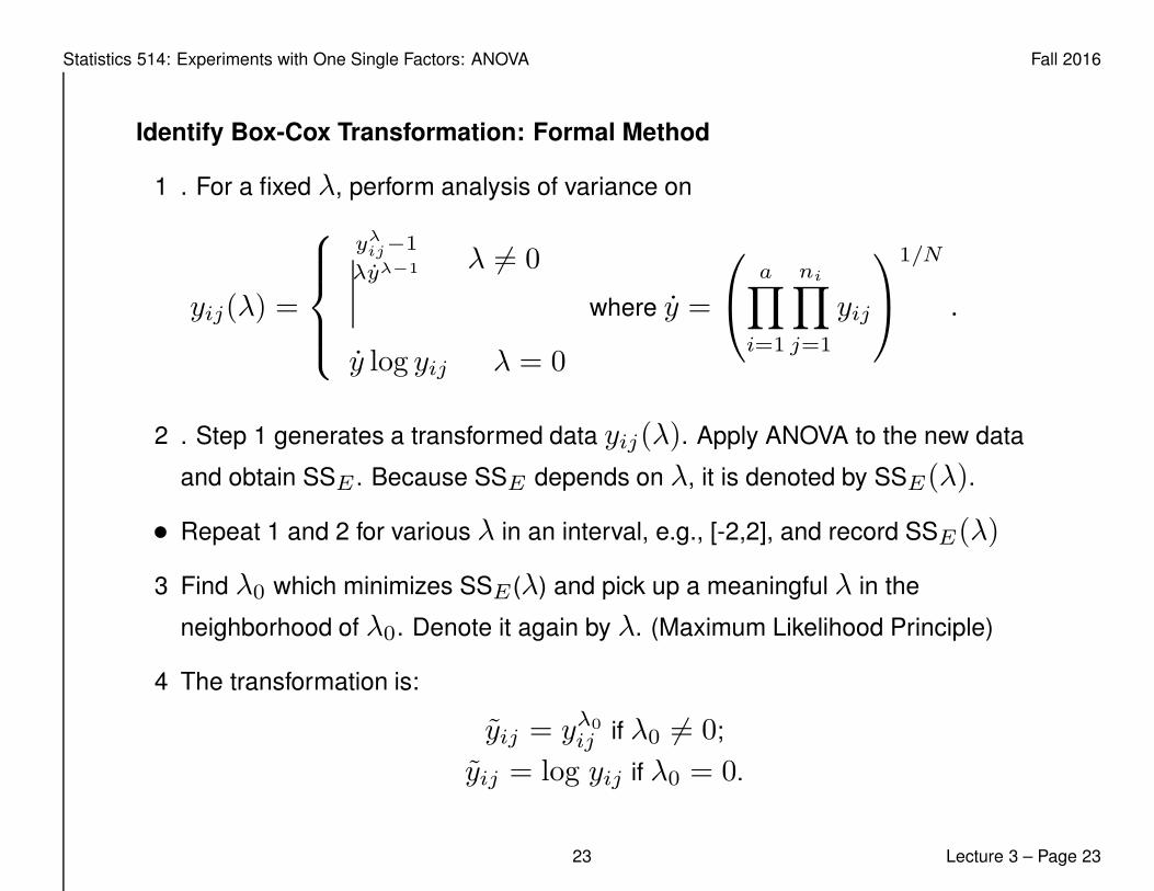
Identify Box-Cox Transformation: Formal Method

1 . For a fixed λ, perform analysis of variance on

yij(λ) =

yλij−1

λyλ−1 λ 6= 0

y log yij λ = 0

where y =

a∏

i=1

ni∏

j=1

yij

1/N

.

2 . Step 1 generates a transformed data yij(λ). Apply ANOVA to the new data

and obtain SSE . Because SSE depends on λ, it is denoted by SSE(λ).

• Repeat 1 and 2 for various λ in an interval, e.g., [-2,2], and record SSE(λ)

3 Find λ0 which minimizes SSE (λ) and pick up a meaningful λ in the

neighborhood of λ0. Denote it again by λ. (Maximum Likelihood Principle)

4 The transformation is:

yij = yλ0

ij if λ0 6= 0;

yij = log yij if λ0 = 0.

23 Lecture 3 –


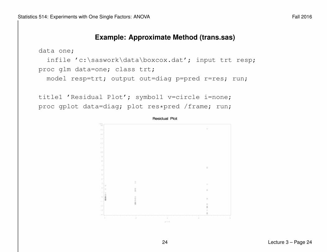
Example: Approximate Method (trans.sas)

data one;

infile ’c:\saswork\data\boxcox.dat’; input trt resp;

proc glm data=one; class trt;

model resp=trt; output out=diag p=pred r=res; run;

title1 ’Residual Plot’; symbol1 v=circle i=none;

proc gplot data=diag; plot res*pred /frame; run;

24 Lecture 3 –


proc univariate data=one noprint;

var resp; by trt; output out=two mean=mu std=sigma;

data three; set two; logmu = log(mu); logsig = log(sigma);

proc reg; model logsig = logmu;

title1 ’Mean vs Std Dev’; symbol1 v=circle i=rl;

proc gplot; plot logsig*logmu / regeqn; run;

25 Lecture 3 –


Example: Formal Method (trans1.sas)

data one;

infile ’c:\saswork\data\boxcox.dat’;

input trt resp;

logresp = log(resp);

proc univariate data=one noprint;

var logresp; output out=two mean=mlogresp;

data three;

set one; if _n_ eq 1 then set two;

ydot = exp(mlogresp);

do l=-2.0 to 2.0 by .25;

den = l*ydot**(l-1); if abs(l) eq 0 then den = 1;

yl=(resp**l -1)/den; if abs(l) < 0.0001 then yl=ydot*log(resp);

output;

end;

keep trt yl l;

proc sort data=three out=three; by l;

26 Lecture 3 –


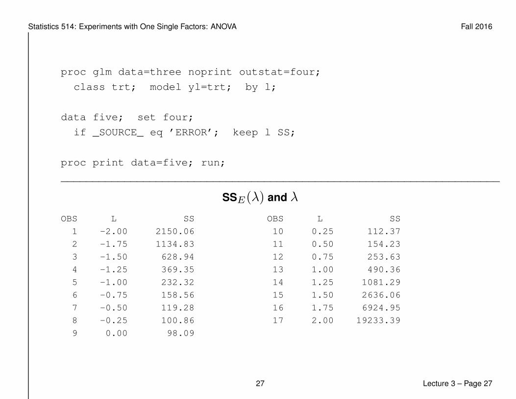
proc glm data=three noprint outstat=four;

class trt; model yl=trt; by l;

data five; set four;

if _SOURCE_ eq ’ERROR’; keep l SS;

proc print data=five; run;

_____________________________________________________________________

SSE(λ) and λ

OBS L SS OBS L SS

1 -2.00 2150.06 10 0.25 112.37

2 -1.75 1134.83 11 0.50 154.23

3 -1.50 628.94 12 0.75 253.63

4 -1.25 369.35 13 1.00 490.36

5 -1.00 232.32 14 1.25 1081.29

6 -0.75 158.56 15 1.50 2636.06

7 -0.50 119.28 16 1.75 6924.95

8 -0.25 100.86 17 2.00 19233.39

9 0.00 98.09

27 Lecture 3 –


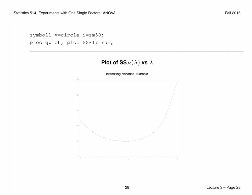
symbol1 v=circle i=sm50;

proc gplot; plot SS*l; run;

_____________________________________________________________________

Plot of SSE(λ) vs λ

28 Lecture 3 –


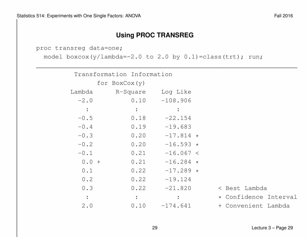
Using PROC TRANSREG

proc transreg data=one;

model boxcox(y/lambda=-2.0 to 2.0 by 0.1)=class(trt); run;

_____________________________________________________________________

Transformation Information

for BoxCox(y)

Lambda R-Square Log Like

-2.0 0.10 -108.906

: : :

-0.5 0.18 -22.154

-0.4 0.19 -19.683

-0.3 0.20 -17.814 *

-0.2 0.20 -16.593 *

-0.1 0.21 -16.067 <

0.0 + 0.21 -16.284 *

0.1 0.22 -17.289 *

0.2 0.22 -19.124

0.3 0.22 -21.820 < Best Lambda

: : : * Confidence Interval

2.0 0.10 -174.641 + Convenient Lambda

29 Lecture 3 –


Kruskal-Wallis Test: a Nonparametric Alternative for Nonnormality

a treatments, H0: a treatments are not different.

• Rank the observations yij in ascending order

• Replace each observation by its rank Rij (assign average for tied

observations), and apply one-way ANOVA to Rij .

• Test statistic (a = 2 =⇒ Wilcoxon rank-sum test)

H = 1S2

[

∑ai=1

R2

i.

ni− N(N+1)2

4

]

≈ χ2a−1 under H0

where S2 = 1N−1

[

∑ai=1

∑ni

j=1R2ij − N(N+1)2

4

]

• Decision Rule: reject H0 if H > χ2α,a−1.

• Let F0 be the F -test statistic in ANOVA based on Rij . Then

F0 =H/(a− 1)

(N − 1−H)/(N − a)

30 Lecture 3 –


A Nonnormality Example

data new;

input strain nitrogen @@;

cards;

1 19.4 1 32.6 1 27.0 1 32.1 1 33.0

2 17.7 2 24.8 2 27.9 2 25.2 2 24.3

3 17.0 3 19.4 3 9.1 3 11.9 3 15.8

4 20.7 4 21.0 4 20.5 4 18.8 4 18.6

5 14.3 5 14.4 5 11.8 5 11.6 5 14.2

6 17.3 6 19.4 6 19.1 6 16.9 6 20.8

;

proc glm data=new;

class strain; model nitrogen=strain;

output out=newres r=res; run;

proc univariate data=newres normal;

var res; qqplot res / normal (L=1 mu=est sigma=est);

run; quit;

31 Lecture 3 –


Tests for Normality

Test Statistic p Value

Shapiro-Wilk W 0.910027 Pr < W 0.0149

Kolmogorov-Smirnov D 0.174133 Pr > D 0.0205

Cramer-von Mises W-Sq 0.155870 Pr > W-Sq 0.0198

Anderson-Darling A-Sq 0.908188 Pr > A-Sq 0.0194

32 Lecture 3 –


proc npar1way data=new; /* May need option: wilcoxon */

class strain; var nitrogen; run;

________________________________________________________________

Analysis of Variance for Variable nitrogen

Classified by Variable strain

Source DF Sum of Squares Mean Square F Value Pr > F

--------------------------------------------------------------

Among 5 847.046667 169.409333 14.3705 <.0001

Within 24 282.928000 11.788667

Kruskal-Wallis Test

Chi-Square 21.6593

DF 5

Pr > Chi-Square 0.0006

Median One-Way Analysis

Chi-Square 13.5333

DF 5

Pr > Chi-Square 0.0189

33 Lecture 3 –


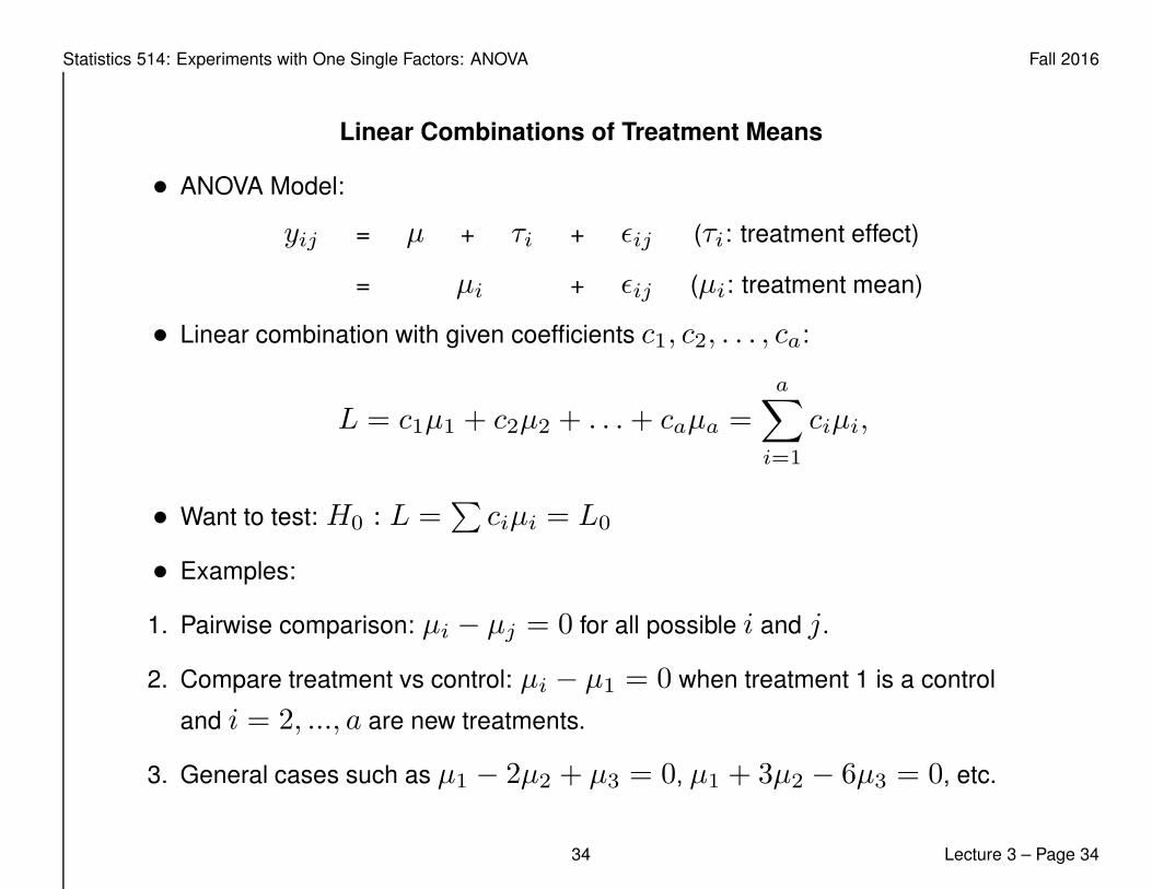
Linear Combinations of Treatment Means

• ANOVA Model:

yij = µ + τi + ǫij (τi: treatment effect)

= µi + ǫij (µi: treatment mean)

• Linear combination with given coefficients c1, c2, . . . , ca:

L = c1µ1 + c2µ2 + . . .+ caµa =a

∑

i=1

ciµi,

• Want to test: H0 : L =∑

ciµi = L0

• Examples:

1. Pairwise comparison: µi − µj = 0 for all possible i and j.

2. Compare treatment vs control: µi − µ1 = 0 when treatment 1 is a control

and i = 2, ..., a are new treatments.

3. General cases such as µ1 − 2µ2 + µ3 = 0, µ1 + 3µ2 − 6µ3 = 0, etc.

34 Lecture 3 –


• Estimate of L:

L =∑

ciµi =∑

ciyi.

Var(L) =∑

c2i Var(yi.) = σ2∑ c2i

ni

(

=σ2

n

∑

c2i

)

• Standard Error of L

S.E.{L} =

√

MSE∑ c2i

ni

• Test statistic

t0 =(L− L0)

S.E.{L}∼ t(N − a) under H0

35 Lecture 3 –


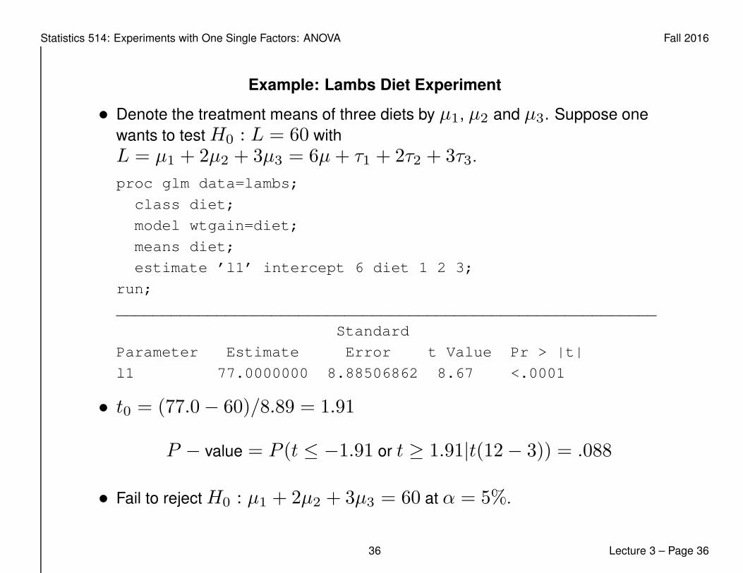
Example: Lambs Diet Experiment

• Denote the treatment means of three diets by µ1, µ2 and µ3. Suppose one

wants to test H0 : L = 60 with

L = µ1 + 2µ2 + 3µ3 = 6µ+ τ1 + 2τ2 + 3τ3.

proc glm data=lambs;

class diet;

model wtgain=diet;

means diet;

estimate ’l1’ intercept 6 diet 1 2 3;

run;

___________________________________________________________

Standard

Parameter Estimate Error t Value Pr > |t|

l1 77.0000000 8.88506862 8.67 <.0001

• t0 = (77.0− 60)/8.89 = 1.91

P − value = P (t ≤ −1.91 or t ≥ 1.91|t(12− 3)) = .088

• Fail to reject H0 : µ1 + 2µ2 + 3µ3 = 60 at α = 5%.

36 Lecture 3 –


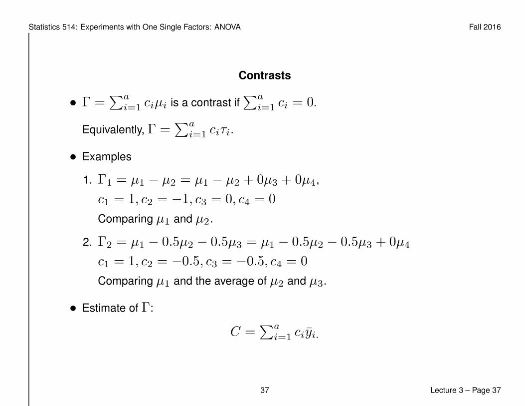
Contrasts

• Γ =∑a

i=1 ciµi is a contrast if∑a

i=1 ci = 0.

Equivalently, Γ =∑a

i=1 ciτi.

• Examples

1. Γ1 = µ1 − µ2 = µ1 − µ2 + 0µ3 + 0µ4,

c1 = 1, c2 = −1, c3 = 0, c4 = 0

Comparing µ1 and µ2.

2. Γ2 = µ1 − 0.5µ2 − 0.5µ3 = µ1 − 0.5µ2 − 0.5µ3 + 0µ4

c1 = 1, c2 = −0.5, c3 = −0.5, c4 = 0

Comparing µ1 and the average of µ2 and µ3.

• Estimate of Γ:

C =∑a

i=1 ciyi.

37 Lecture 3 –


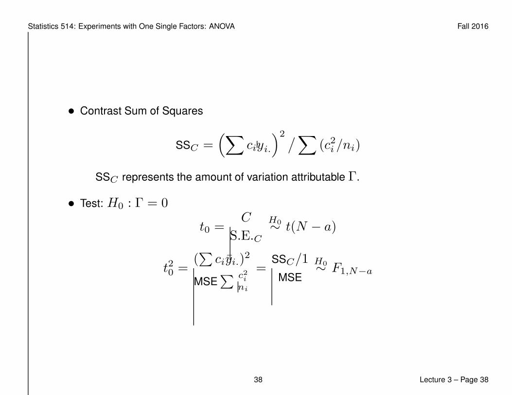
• Contrast Sum of Squares

SSC =(

∑

ciyi.

)2/

∑

(c2i /ni)

SSC represents the amount of variation attributable Γ.

• Test: H0 : Γ = 0

t0 =C

S.E.C

H0∼ t(N − a)

t20 =(∑

ciyi.)2

MSE∑ c2

i

ni

=SSC/1

MSE

H0∼ F1,N−a

38 Lecture 3 –


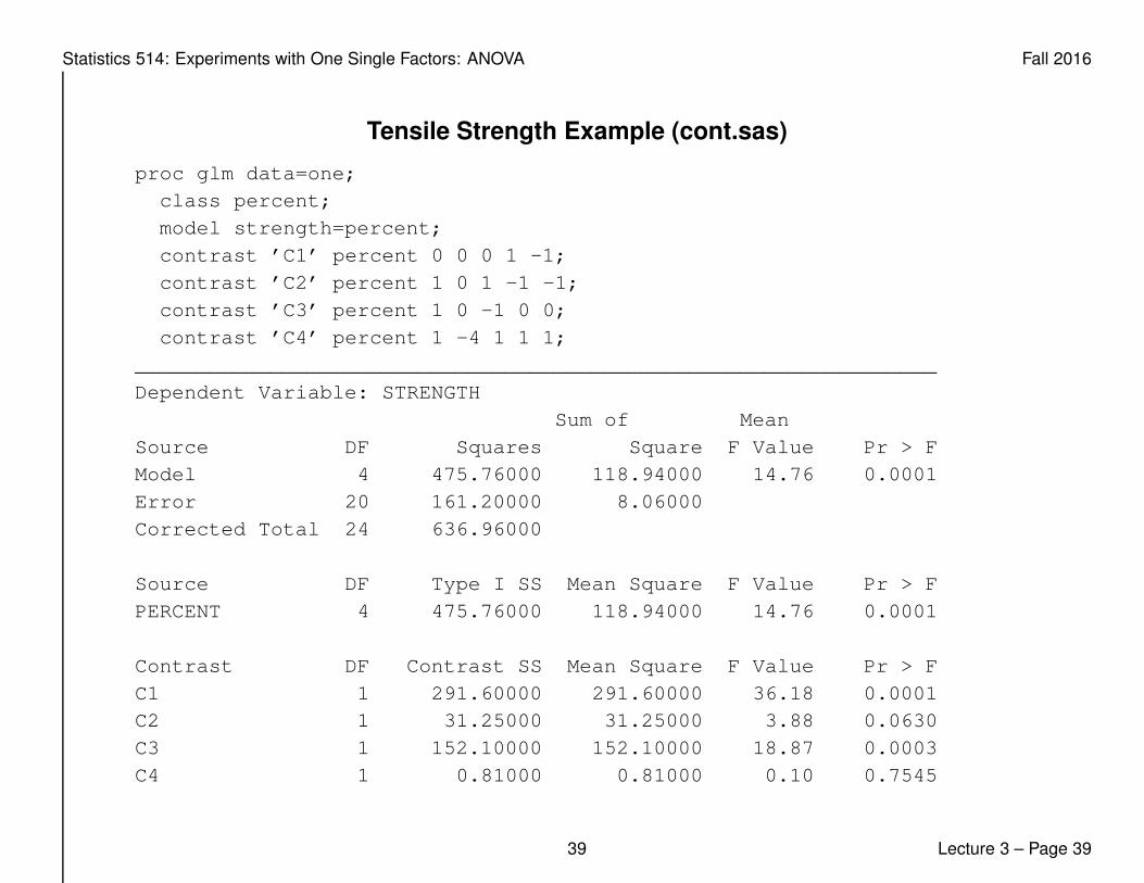
Tensile Strength Example (cont.sas)

proc glm data=one;

class percent;

model strength=percent;

contrast ’C1’ percent 0 0 0 1 -1;

contrast ’C2’ percent 1 0 1 -1 -1;

contrast ’C3’ percent 1 0 -1 0 0;

contrast ’C4’ percent 1 -4 1 1 1;

_________________________________________________________________

Dependent Variable: STRENGTH

Sum of Mean

Source DF Squares Square F Value Pr > F

Model 4 475.76000 118.94000 14.76 0.0001

Error 20 161.20000 8.06000


Source DF Type I SS Mean Square F Value Pr > F

PERCENT 4 475.76000 118.94000 14.76 0.0001

Contrast DF Contrast SS Mean Square F Value Pr > F

C1 1 291.60000 291.60000 36.18 0.0001

C2 1 31.25000 31.25000 3.88 0.0630

C3 1 152.10000 152.10000 18.87 0.0003

C4 1 0.81000 0.81000 0.10 0.7545

39 Lecture 3 –


Orthogonal Contrasts

• Two contrasts {ci} and {di} are Orthogonal if

a∑

i=1

cidini

= 0 (a

∑

i=1

cidi = 0 for balanced experiments)

• Example (Balanced Experiment)

Γ1 = µ1 + µ2 − µ3 − µ4, So c1 = 1, c2 = 1, c3 = −1, c4 = −1.

Γ2 = µ1 − µ2 + µ3 − µ4. So d1 = 1, d2 = −1, d3 = 1, d4 = −1

It is easy to verify that both Γ1 and Γ2 are contrasts. Furthermore,

c1d1 + c2d2 + c3d3 + c4d4 =

1× 1 + 1× (−1) + (−1)× 1 + (−1)× (−1) = 0. Hence, Γ1 and Γ2

are orthogonal to each other.

• A complete set of orthogonal contrasts C = {Γ1,Γ2, . . . ,Γa−1} if

contrasts are mutually orthogonal and there does not exist a contrast

orthogonal outside of C to all the contrasts in C.

40 Lecture 3 –


• If there are a treatments, C must contain a− 1 contrasts.

• Complete set is not unique. For example, in the tensile strength example

C1 : includes :

Γ1 = (0, 0, 0, 1, −1)

Γ2 = (1, 0, 1, −1, −1)

Γ3 = (1, 0, −1, 0, 0)

Γ4 = (1, −4, 1, 1, 1)

C2 : includes :

Γ′1 = (−2, −1, 0, 1, 2)

Γ′2 = (2, −1, −2, −1, 2)

Γ′3 = (−1, 2, 0, −2, 1)

Γ′4 = (1, −4, 6, −4, 1)

41 Lecture 3 –


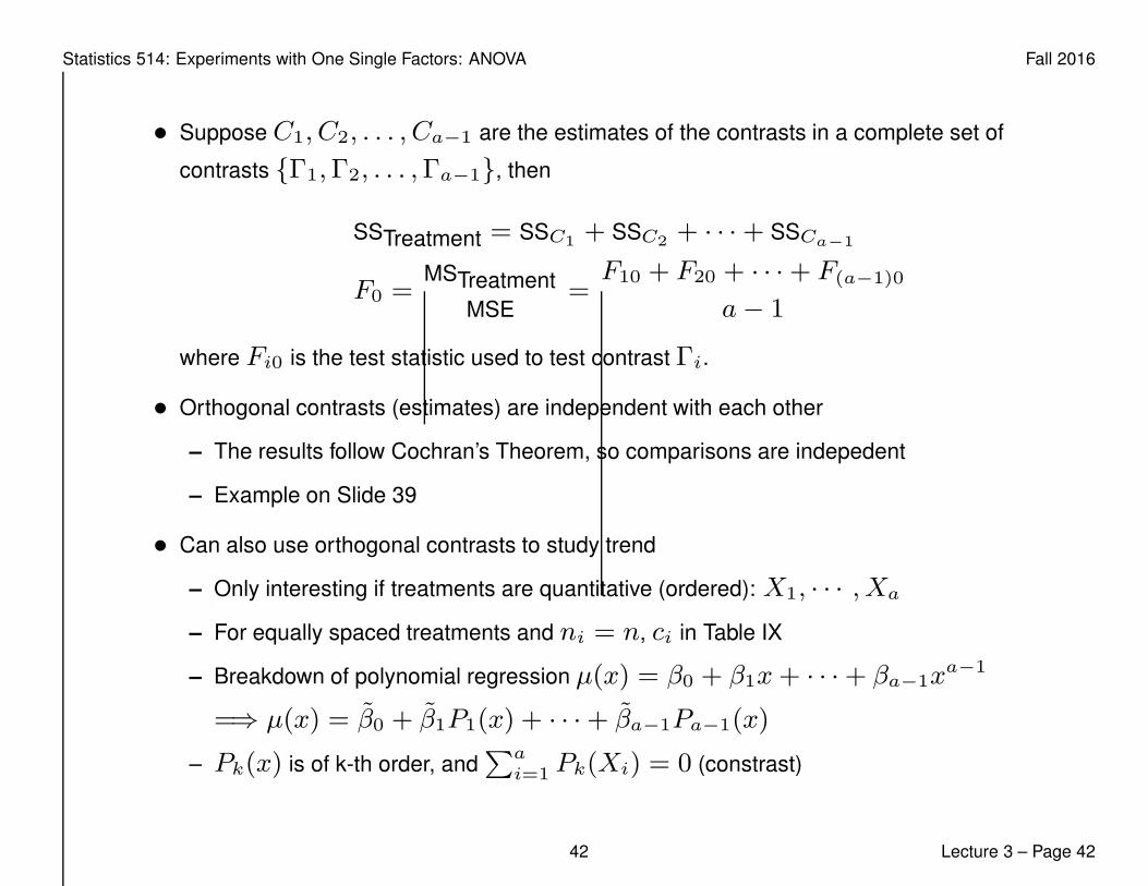
• Suppose C1, C2, . . . , Ca−1 are the estimates of the contrasts in a complete set of

contrasts {Γ1,Γ2, . . . ,Γa−1}, then

SSTreatment = SSC1+ SSC2

+ · · ·+ SSCa−1

F0 =MSTreatment

MSE=

F10 + F20 + · · ·+ F(a−1)0

a− 1

where Fi0 is the test statistic used to test contrast Γi.

• Orthogonal contrasts (estimates) are independent with each other

– The results follow Cochran’s Theorem, so comparisons are indepedent

– Example on Slide 39

• Can also use orthogonal contrasts to study trend

– Only interesting if treatments are quantitative (ordered): X1, · · · , Xa

– For equally spaced treatments and ni = n, ci in Table IX

– Breakdown of polynomial regression µ(x) = β0 + β1x+ · · ·+ βa−1xa−1

=⇒ µ(x) = β0 + β1P1(x) + · · ·+ βa−1Pa−1(x)

– Pk(x) is of k-th order, and∑a

i=1 Pk(Xi) = 0 (constrast)

42 Lecture 3 –


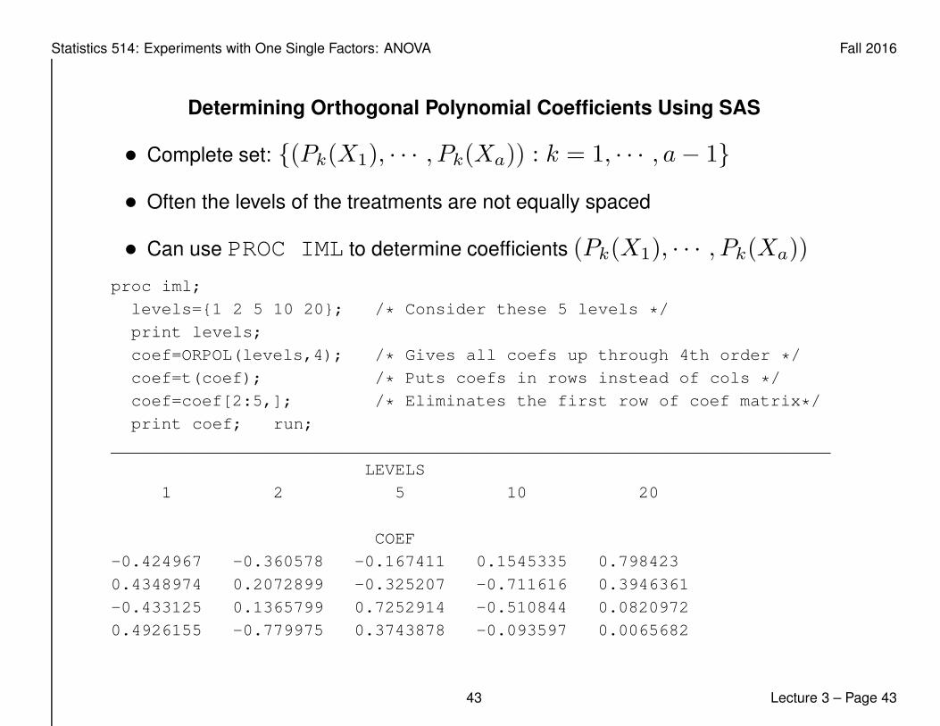
Determining Orthogonal Polynomial Coefficients Using SAS

• Complete set: {(Pk(X1), · · · , Pk(Xa)) : k = 1, · · · , a− 1}

• Often the levels of the treatments are not equally spaced

• Can use PROC IML to determine coefficients (Pk(X1), · · · , Pk(Xa))

proc iml;

levels={1 2 5 10 20}; /* Consider these 5 levels */

print levels;

coef=ORPOL(levels,4); /* Gives all coefs up through 4th order */

coef=t(coef); /* Puts coefs in rows instead of cols */

coef=coef[2:5,]; /* Eliminates the first row of coef matrix*/

print coef; run;

_______________________________________________________________________

LEVELS

1 2 5 10 20

COEF

-0.424967 -0.360578 -0.167411 0.1545335 0.798423

0.4348974 0.2072899 -0.325207 -0.711616 0.3946361

-0.433125 0.1365799 0.7252914 -0.510844 0.0820972

0.4926155 -0.779975 0.3743878 -0.093597 0.0065682

43 Lecture 3 –


Testing Multiple Contrasts (Multiple Comparisons)

• One contrast:

H0 : Γ =∑

ciµi = Γ0 vs H1 : Γ 6= Γ0 at α

100(1-α) Confidence Interval (CI) for Γ:

CI :∑

ciyi. ± tα/2,N−a

√

MSE

∑ c2ini

P (CI does not contain L0|H0) = α(= type I error rate)

• Decision Rule: Reject H0 if CI does not contain Γ0.

44 Lecture 3 –


• Multiple contrasts, for i = 1, 2, · · · ,m,

H(i)0 : Γ(i) = Γ

(i)0 , vs H

(i)1 : Γ(i) 6= Γ

(i)0

If we construct CI1, CI2,..., CIm, each with 100(1-α) level, then for each CIi,

P (rejectH(i)0 | H(i)

0 ) = P (CIi does not contain Γ(i)0 | H(i)

0 ) = α

• But the overall Type I error rate (probability of any type I error in testing

H(i)0 vs H

(i)1 , i = 1, · · · ,m) is inflated and much larger than α, that is,

P (reject at least one of {H(i)0 , i = 1, · · · ,m} | H(1)

0 , · · · , H(m)0 )

= P (at least one CIi do not contain Γ(i)0 | H(1)

0 , · · · , H(m)0 )

≫ α

• One way to achieve small overall error rate, we require much smaller error

rate (α′) of each individual CIi.

45 Lecture 3 –


Bonferroni Method for Testing Multiple Contrasts

• Bonferroni Inequality

P (reject at least one of {H(i)0 , i = 1, · · · ,m} | H

(1)0 , · · · , H

(m)0 )

= P (reject H(1)0 or reject H

(2)0 or ... or reject H

(m)0 | H

(1)0 , · · · , H

(m)0 )

≤ P (reject H(1)0 | H

(1)0 ) + · · ·+ P (reject H

(m)0 | H

(m)0 ) = mα′

• In order to control overall error rate (or, overall confidence level), let

mα′ = α,we have, α′ = α/m

• Bonferroni CIs:

CIi :∑

cij yj. ± tα/2m(N − a)

√

MSE

∑ c2ijnj

• When m is large, Bonferroni CIs are too conservative ( overall type II error too large).

46 Lecture 3 –


Scheffe’s Method for Testing All Contrasts

• Consider all possible contrasts: Γ =∑

ciµi

Estimate: C =∑

ciyi., St. Error: S.E.C =√

MSE∑ c2

i

ni

• Critical value:√

(a− 1)Fα,a−1,N−a

• Scheffe’s simultaneous CI: C ±√

(a− 1)Fα,a−1,N−a S.E.C

• Overall confidence level and error rate for m contrasts

P (CIs contain true parameter for any contrast) ≥ 1− α

P (at least one CI does not contain true parameter) ≤ α

Remark: Scheffe’s method is also conservative, too conservative when m is

small

47 Lecture 3 –


Methods for Pairwise Comparisons

• There are a(a− 1)/2 possible pairs: µi − µj (contrast for comparing µi

and µj ). We may be interested in m pairs or all pairs.

• Standard Procedure:

1. Estimation: yi. − yj.

2. Compute a Critical Difference (CD) (based on the method employed)

3. If

| yi. − yj. |> CD

or equivalently if the interval

(yi. − yj. − CD, yi. − yj. +CD)

does not contain zero, declare µi − µj significant.

48 Lecture 3 –


Methods for Calculating CD

• Least significant difference (LSD):

CD = tα/2,N−a

√

MSE(1/ni + 1/nj)

not control overall error rate

• Bonferroni method (for m pairs)

CD = tα/2m,N−a

√

MSE(1/ni + 1/nj)

control overall error rate for the m comparisons.

• Tukey’s method (for all possible pairs)

CD =qα(a,N − a)√

2

√

MSE(1/ni + 1/nj)

qα(a,N − a) from studentized range distribution (Table VII). Control overall

error rate (exact for balanced experiments). (Example 3.7).

49 Lecture 3 –


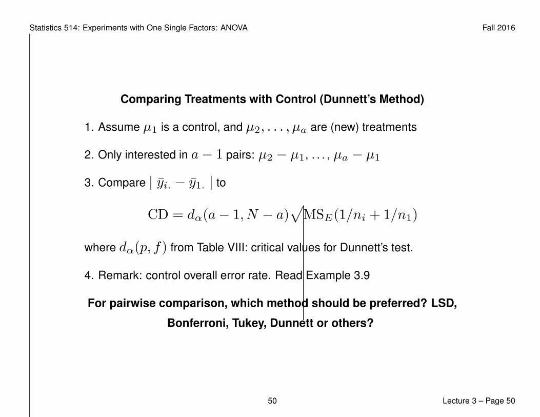
Comparing Treatments with Control (Dunnett’s Method)

1. Assume µ1 is a control, and µ2, . . . , µa are (new) treatments

2. Only interested in a− 1 pairs: µ2 − µ1, . . . , µa − µ1

3. Compare | yi. − y1. | to

CD = dα(a− 1, N − a)√

MSE(1/ni + 1/n1)

where dα(p, f) from Table VIII: critical values for Dunnett’s test.

4. Remark: control overall error rate. Read Example 3.9

For pairwise comparison, which method should be preferred? LSD,

Bonferroni, Tukey, Dunnett or others?

50 Lecture 3 –


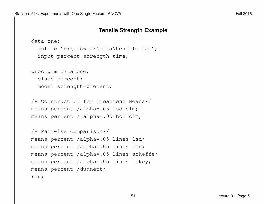
Tensile Strength Example

data one;

infile ’c:\saswork\data\tensile.dat’;

input percent strength time;

proc glm data=one;

class percent;

model strength=precent;

/* Construct CI for Treatment Means*/

means percent /alpha=.05 lsd clm;

means percent / alpha=.05 bon clm;

/* Pairwise Comparison*/

means percent /alpha=.05 lines lsd;

means percent /alpha=.05 lines bon;

means percent /alpha=.05 lines scheffe;

means percent /alpha=.05 lines tukey;

means percent /dunnett;

run;

51 Lecture 3 –


The GLM Procedure

t Confidence Intervals for y

Alpha 0.05

Error Degrees of Freedom 20

Error Mean Square 8.06

Critical Value of t 2.08596

Half Width of Confidence Interval 2.648434

95% Confidence

trt N Mean Limits

30 5 21.600 18.952 24.248

25 5 17.600 14.952 20.248

20 5 15.400 12.752 18.048

35 5 10.800 8.152 13.448

15 5 9.800 7.152 12.448

52 Lecture 3 –


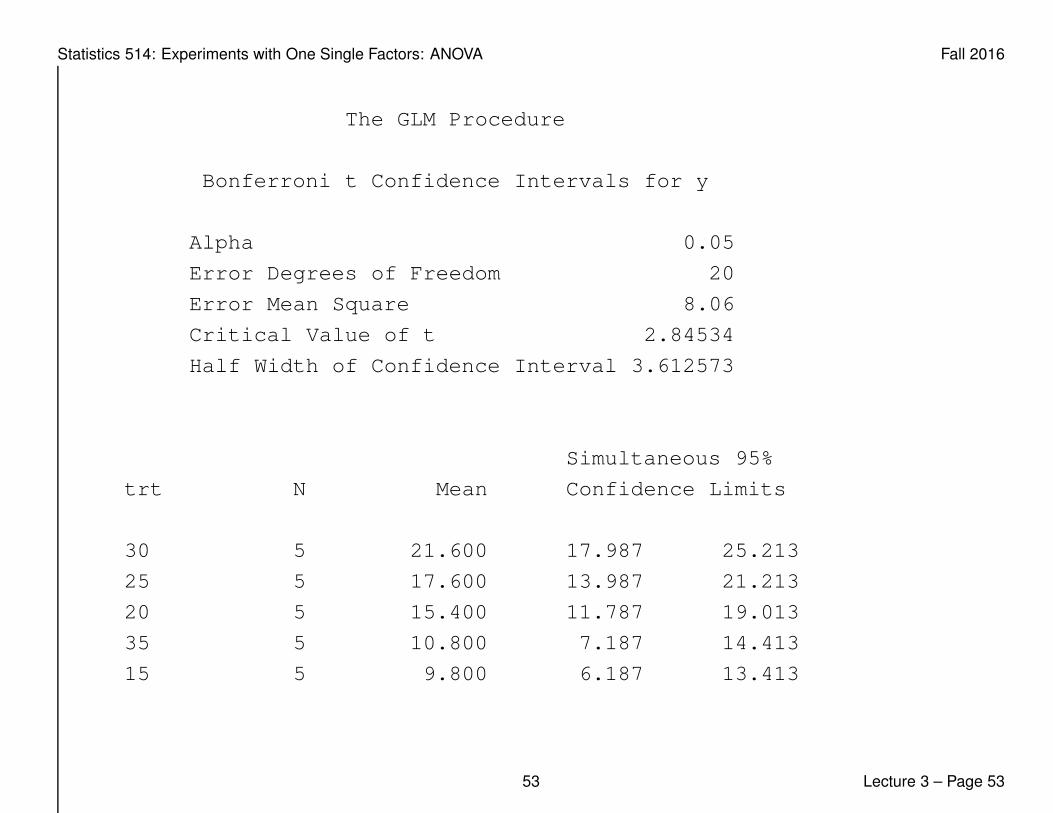
The GLM Procedure

Bonferroni t Confidence Intervals for y

Alpha 0.05




Half Width of Confidence Interval 3.612573

Simultaneous 95%

trt N Mean Confidence Limits

30 5 21.600 17.987 25.213

25 5 17.600 13.987 21.213

20 5 15.400 11.787 19.013

35 5 10.800 7.187 14.413

15 5 9.800 6.187 13.413

53 Lecture 3 –


t Tests (LSD) for y

NOTE: This test controls the Type I comparisonwise error rate, not

the experimentwise error rate.

Alpha 0.05




Least Significant Difference 3.7455

Means with the same letter are not significantly different.

t Grouping Mean N trt

A 21.600 5 30

B 17.600 5 25

B 15.400 5 20

C 10.800 5 35

C 9.800 5 15

54 Lecture 3 –


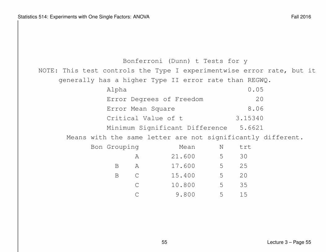
Bonferroni (Dunn) t Tests for y

NOTE: This test controls the Type I experimentwise error rate, but it

generally has a higher Type II error rate than REGWQ.

Alpha 0.05




Minimum Significant Difference 5.6621


Bon Grouping Mean N trt

A 21.600 5 30

B A 17.600 5 25

B C 15.400 5 20

C 10.800 5 35

C 9.800 5 15

55 Lecture 3 –


Scheffe’s Test for y

NOTE: This test controls the Type I experimentwise error rate.

Alpha 0.05



Critical Value of F 2.86608



Scheffe Grouping Mean N trt

A 21.600 5 30

A

B A 17.600 5 25

B

B C 15.400 5 20

C

C 10.800 5 35

C

C 9.800 5 15

56 Lecture 3 –


Tukey’s Studentized Range (HSD) Test for y

NOTE: This test controls the Type I experimentwise error rate, but it

generally has a higher Type II error rate than REGWQ.

Alpha 0.05



Critical Value of Studentized Range 4.23186



Tukey Grouping Mean N trt

A 21.600 5 30

A

B A 17.600 5 25

B

B C 15.400 5 20

C

D C 10.800 5 35

D

D 9.800 5 15

57 Lecture 3 –


Dunnett’s t Tests for y

NOTE: This test controls the Type I experimentwise error for

comparisons of all treatments against a control.

Alpha 0.05



Critical Value of Dunnett’s t 2.65112


Comparisons significant at the 0.05 level are indicated by ***.

Difference

trt Between Simultaneous 95%

Comparison Means Confidence Limits

30 - 15 11.800 7.040 16.560 ***

25 - 15 7.800 3.040 12.560 ***

20 - 15 5.600 0.840 10.360 ***

35 - 15 1.000 -3.760 5.760

58 Lecture 3 –

lecture 3. experiments with a single factor: anovaminzhang/514_fall2016/lec...

Documents