lecture 3 - first morphometric analysis

Department of Geological Sciences | Indiana University (c) 2012, P. David Polly

G562 Geometric Morphometrics

A

BCDE

F G

H

I

J K L

Mathematica map of Marmot localities from Assignment 1

First analysisGeometric Morphometrics



Tips for data manipulation in Mathematica

Flatten[ ] - Takes a nested list and flattens it into a single list.

Partition[ ] - Opposite of flatten: groups items into a nested list.

Transpose[ ] - Switches columns to rows and rows to columns.



Taking rows and columns of data in Mathematica

Double square brackets after a variable allow you to select parts of a list or matrix. For these examples, data is a matrix with ten rows and seven columns.

The first number in the brackets indicates rows, the second number indicates columns.

The code for taking the highlighted data is shown beneath each example.

Mathematica code: data[[5, 2]]

Example 1: take column 2 of row 5

Mathematica code: data[[4]]

Example 2: take all of row 4



Taking rows and columns (cont.)

Mathematica code: data[[3;;]]

Example 3: take rows 3 to the last row

Mathematica code: data[[3;;6]]

Example 4: take rows 3 through 6

Mathematica code: data[[{3,6}]]

Example 5: take rows 3 then 6

Mathematica code: data[[1;;,1]]

Example 6: take column 1




Mathematica code: data[[1;;,3;;]]

Example 7: take columns 3 through the end

Mathematica code: data[[1;;,3;;5]]

Example 8: take columns 3 through 5

Mathematica code: data[[1;;8,3;;5]]

Example 9: take rows 4 through 8 in columns 3 through 5

Mathematica code: data[[1;;,{3,6}]]

Example 10: take columns 3 then 6




Mathematica code: data[[1;;,{6,3}]]

Example 11: take columns 6 then 3

Mathematica code: data[[1;;6,{2,4,6}]]

Example 12: take rows 1 - 6 of columns 2, 4, and 6



Taking longitude and latitude from Assignment 1

For the map assignment you needed longitude and latitude from the table stored in data. Furthermore, you need longitude in your first column because it should be on the horizontal x-axis, whereas latitude should be in the second column so it will appear on the y-axis. You also need to discard the first row because it contains column labels instead of numbers.

Mathematica code: data[[2;;, {9,8}]]



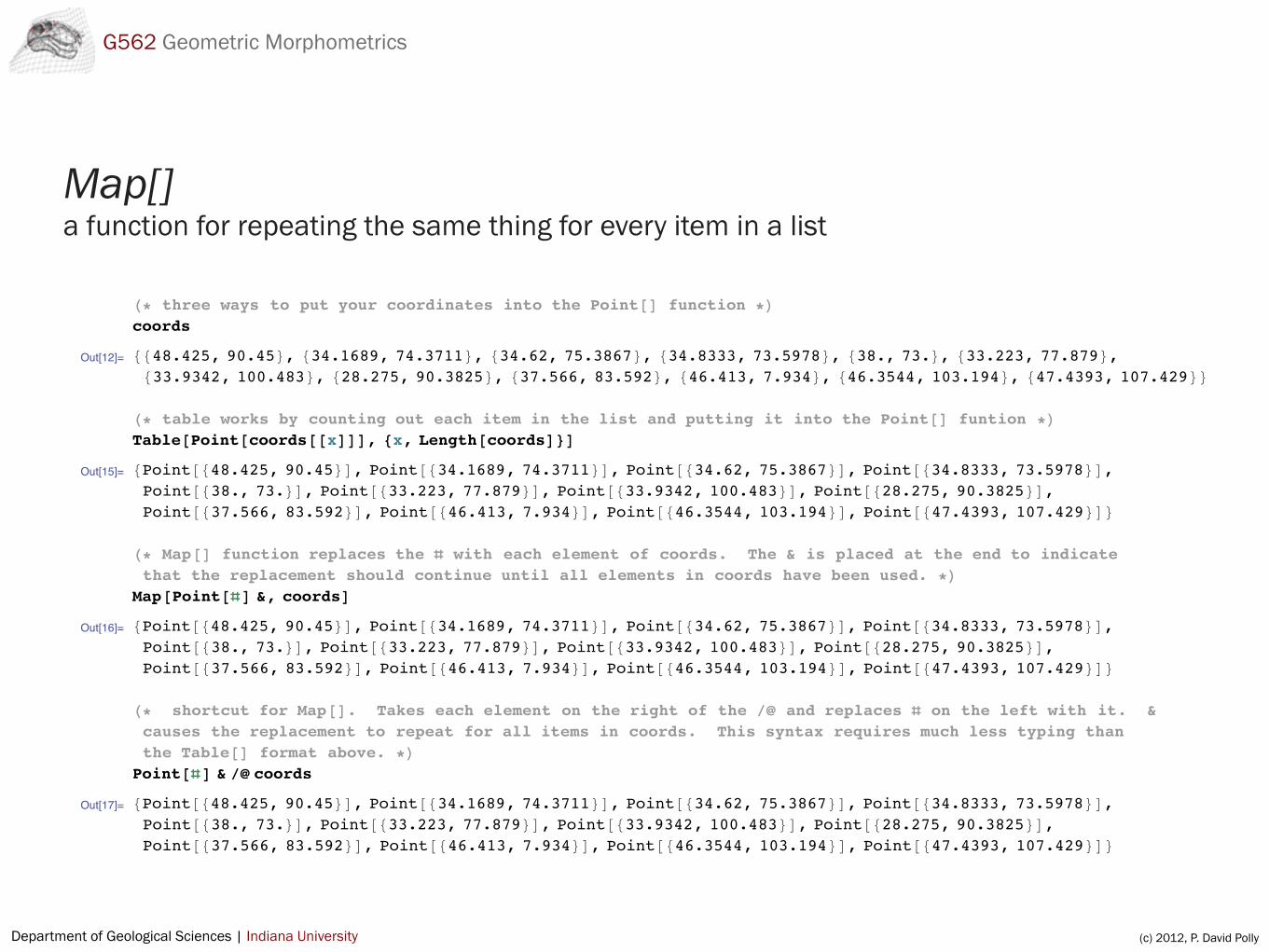
Map[] a function for repeating the same thing for every item in a list

H* three ways to put your coordinates into the Point@D function *Lcoords

Out[12]= 8848.425, 90.45<, 834.1689, 74.3711<, 834.62, 75.3867<, 834.8333, 73.5978<, 838., 73.<, 833.223, 77.879<,833.9342, 100.483<, 828.275, 90.3825<, 837.566, 83.592<, 846.413, 7.934<, 846.3544, 103.194<, 847.4393, 107.429<<H* table works by counting out each item in the list and putting it into the Point@D funtion *LTable@Point@coords@@xDDD, 8x, Length@coordsD<D

Out[15]= [email protected], 90.45<D, [email protected], 74.3711<D, [email protected], 75.3867<D, [email protected], 73.5978<D,Point@838., 73.<D, [email protected], 77.879<D, [email protected], 100.483<D, [email protected], 90.3825<D,[email protected], 83.592<D, [email protected], 7.934<D, [email protected], 103.194<D, [email protected], 107.429<D<

H* Map@D function replaces the with each element of coords. The & is placed at the end to indicatethat the replacement should continue until all elements in coords have been used. *L

Map@Point@D &, coordsDOut[16]= [email protected], 90.45<D, [email protected], 74.3711<D, [email protected], 75.3867<D, [email protected], 73.5978<D,

Point@838., 73.<D, [email protected], 77.879<D, [email protected], 100.483<D, [email protected], 90.3825<D,[email protected], 83.592<D, [email protected], 7.934<D, [email protected], 103.194<D, [email protected], 107.429<D<

H* shortcut for Map@D. Takes each element on the right of the êû and replaces on the left with it. &causes the replacement to repeat for all items in coords. This syntax requires much less typing thanthe Table@D format above. *L

Point@D & êû coordsOut[17]= [email protected], 90.45<D, [email protected], 74.3711<D, [email protected], 75.3867<D, [email protected], 73.5978<D,

Point@838., 73.<D, [email protected], 77.879<D, [email protected], 100.483<D, [email protected], 90.3825<D,[email protected], 83.592<D, [email protected], 7.934<D, [email protected], 103.194<D, [email protected], 107.429<D<



Steps in a Geometric Morphometric Methods (GMM) Analysis

1. Collect landmark coordinates

2. Do a Procrustes superimposition

Standardizes landmarks by rescaling them and rotating them to a common orientation using least-squares fitting

3. Analyze similarity and difference of shape

Analysis usually starts with a Principal Components Analysis, which (A) shows similarity and differences as simple scatter plots, and (B) provides new variables for further statistical analysis



Performing a GMM analysis in Mathematica

GMM functions are in the Polly Morphometrics add-in package for Mathematica

1. Download the latest version of the package at http://mypage.iu.edu/~pdpolly/Software.html (right click on link to save as file)

2. Open the file in Mathematica

3. From the File menu, choose “Install”

4. From “Type of Item” choose “Package”, from “Source” choose “PollyMorphometrics8.x.m”, under “Install Name” choose a short name for the package (e.g., “PollyMorphometrics”)

5. Once installed, enter the command “<<PollyMorphometrics`” to use the functions

For detailed information about the functions, see the Guide to Morphometrics for Mathematica available from the same web page.

http://mypage.iu.edu/~pdpolly/Software.html



Step 1: Collecting landmarks1. Each image must have the same number of landmarks;

2. The landmarks on each image must be in the same order;

3. Landmarks are ordinarily placed on homologous points, points that can be replicated from object to object based on common morphology, common function, or common geometry.

1

2

3

4

5

13

12

11 8

10 9

7

6

Osteostracan head shield from Sansom, 2009



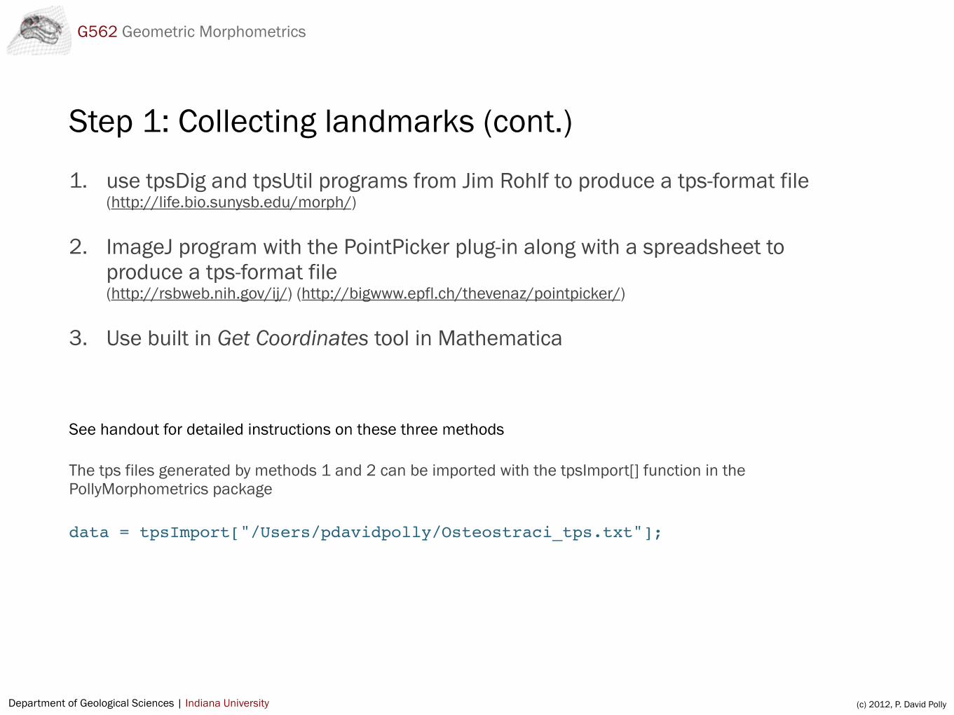
Step 1: Collecting landmarks (cont.)

1. use tpsDig and tpsUtil programs from Jim Rohlf to produce a tps-format file(http://life.bio.sunysb.edu/morph/)

2. ImageJ program with the PointPicker plug-in along with a spreadsheet to produce a tps-format file(http://rsbweb.nih.gov/ij/) (http://bigwww.epfl.ch/thevenaz/pointpicker/)

3. Use built in Get Coordinates tool in Mathematica

See handout for detailed instructions on these three methods

The tps files generated by methods 1 and 2 can be imported with the tpsImport[] function in the PollyMorphometrics package

data = tpsImport["/Users/pdavidpolly/Osteostraci_tps.txt"];

http://life.bio.sunysb.edu/morph/





Step 2: Procrustes superimposition

Procrustes superimposition is the “standardization” step in GMM.

Procrustes removes (1) size, (2) translation, (3) rotation from the original landmark data. In other words, it centers them all together, scales them to the same size, and rotates them into the same orientation.

The Procrustes step removes statistical degrees of freedom from your data, which has implications for later statistical analyses.

After landmarks have been superimposed, the similarities and differences in their shape can be analyzed.



Step 2: Procrustes (cont.)Once you have your landmarks, arrange them in a matrix where each row is a different object, and each column is a landmark coordinate. There should be no column labels.

260 6 258 141 259 167 260 305 259 388 445 395 403 263 308 45 297 168 222 168 217 51 118 264 76 394192 6 188 88 188 111 191 164 192 206 370 158 294 156 220 27 211 111 171 111 165 29 96 157 15 156161 23 158 206 159 229 160 269 157 292 313 227 198 250 182 171 172 227 148 229 137 171 120 250 5 227180 16 179 150 182 186 177 230 178 241 349 236 235 219 204 105 198 184 163 185 158 107 126 221 9 239152 11 150 99 152 121 151 209 147 268 262 279 284 210 198 40 171 120 129 122 109 42 30 211 52 283189 12 190 88 194 106 193 158 191 214 381 262 378 236 235 34 221 104 164 101 153 32 8 233 6 264148 2 146 100 148 123 148 206 147 246 269 290 269 211 174 33 176 125 123 127 122 37 25 214 31 290150 8 148 76 152 89 149 137 150 226 295 275 258 164 166 25 167 87 131 91 135 29 47 160 10 271135 5 134 221 133 252 136 314 132 342 242 259 196 281 155 149 154 253 118 253 114 147 71 280 30 258270 9 271 88 272 101 269 162 268 226 535 261 440 165 308 32 294 99 250 101 235 34 100 160 13 273161 1 163 46 163 70 163 123 163 190 300 203 290 147 194 23 187 70 141 71 132 25 37 146 20 204

Save that matrix in a variable called data then superimpose the landmarks using the Procrustes[] function:

proc = Procrustes[data, 13, 2]

where 13 is the number of landmarks and 2 indicates they are two-dimensional.

HINT: Don’t know how many landmarks? Count them by finding out the length of elements in one row (i.e., the number of columns) and divide by two: Length[data[[1]]] / 2



Step 3: Principal Components AnalysisPrincipal Components Analysis (PCA) ordinates the objects in your analysis by arranging them in a shape space. Similarities and differences can easily be seen in a PCA plot.

The axes of a PCA plot are Principal Components (PCs). The first PC of any analysis is, by definition, the one that shows the largest axis of variation in shape. The second PC shows the next largest axis of variation that is uncorrelated with the first, the third PC shows the third largest axis of variation, and so on.

Each point on a PCA plot represents the shape of a single object from your analysis. The closer two objects are, the more similar they are in shape.

Ateleaspis_tesselata

Benneviaspis_lankesteri

Boreaspis_ceratopsDicranaspis_gracilis

Hirella_gracilis

Parameteroaspis_gigis

Pattenaspis_acuminata

Scolenaspis_signata

Spatulaspis_costata

Stensiopelta_pustulata

Zenaspis_salweyi

-0.6 -0.4 -0.2 0.0 0.2

-0.3

-0.2

-0.1

0.0

0.1

0.2

0.3

PC 1

PC2

PCA Plot



Step 3: PCA (cont.)A PCA plot is often called a morphospace in GMM because each point on the plot represents a different shape or, more specifically, a different configuration of landmarks. An important part of understanding PCA results is to explore how shape varies in the PCA plot.

The thin-plate spline grids in this PCA plot show how shape varies along PC1 and PC2 for a data set of osteostracan fish head shields (shown at right). For example, at the left of the plot landmark 1 is located far in front of 8 and 11, at the right it is very close to 8 and 11. The species at the left of the plot on the previous slide have shapes like the grids on the left in this plot. Exploring morphospace with these grids can help understand the meaning of the PCA.

1

2

3

4

5

13

12

11 8

10 9

7

6

-1.0 -0.8 -0.6 -0.4 -0.2 0.0 0.2 0.4

-0.4

-0.2

0.0

0.2

0.4

PC 1

PC2

Morphospace

PCA Plot



Step 3: PCA (cont.)You can also explore the distribution of shape by referring back to your original photographs.

Compare these shapes to the grids on the previous slide.

Ateleaspis_tesselata

Benneviaspis_lankesteri

Boreaspis_ceratopsDicranaspis_gracilis

Hirella_gracilis

Parameteroaspis_gigis

Pattenaspis_acuminata

Scolenaspis_signata

Spatulaspis_costata

Stensiopelta_pustulata

Zenaspis_salweyi

-0.6 -0.4 -0.2 0.0 0.2

-0.3

-0.2

-0.1

0.0

0.1

0.2

0.3

PC 1

PC2

PCA Plot

1

2

3

4

5

13

12

11 8

10 9

7

6



Step 3: PCA (cont.)

To do a PCA of shape in Mathematica:

PrincipalComponentsOfShape[proc, {1,2}, labels]

where proc is matrix of Procrustes superimposed coordinates from Step 2, the list {1,2} tells the function to plot the first and second principal components, and labels is a list of text labels for each object in proc.

This function provides the following output:

1. A PCA plot showing the objects with labels

2. Text output explaining how much of the variation in shape is explained by each PC

3. A graphic representation of the mean shape in your data set, where each landmark is indicated by its number and a convex hull has been placed around the landmarks

4. A morphospace model showing thin-plate spline snapshots of shape variation in the PCA plot.



Step 3: PCA (cont.)

13

12

11

102

5

1

4

3 9

8

7

6

Mean Shape

1

2

3

4

5

13

12

11 8

10 9

7

6



Assignment 2 - “Faces” project1. Download the face photographs from Oncourse

2. Choose a landmark scheme for the faces, remembering that you must place the same number of landmarks on each face and they must always be placed in the same order.

3. Import the landmarks into Mathematica.

4. Superimpose them with the Procrustes[] function.

5. Do a Principal Components Analysis of Shape on your Procrustes superimposed landmarks.

6. Study the results to determine what the major axes of your PCA plot show, and to decide whether the results accurately pick up differences in people’s facial features or whether other biases affect the outcome of the analysis.

7. Turn in Assignment 2. We will discuss results next week in class.

lecture 3 - first morphometric analysis

Documents