lecture 3: multi-class classification · previous lecture vbinary linear classification models...

Lecture 3:Multi-Class Classification

Kai-Wei ChangCS @ UCLA

[email protected]

Couse webpage: https://uclanlp.github.io/CS269-17/

1ML in NLP

Previous Lecture

v Binary linear classification modelsv Perceptron, SVMs, Logistic regression

v Prediction is simple:v Given an example 𝑥, prediction is 𝑠𝑔𝑛 𝑤&xv Note that all these linear classifier have the same

inference rulev In logistic regression, we can further estimate the

probability

v Question?2CS6501 Lecture 3

This Lecture

vMulticlass classification overviewvReducing multiclass to binary

vOne-against-all & One-vs-onevError correcting codes

vTraining a single classifier vMulticlass Perceptron: Kesler’s constructionvMulticlass SVMs: Crammer&Singer formulationvMultinomial logistic regression

CS6501 Lecture 3 3

What is multiclass

v Output ∈ 1,2,3, …𝐾v In some cases, output space can be very large

(i.e., K is very large)v Each input belongs to exactly one class

(c.f. in multilabel, input belongs to many classes)

CS6501 Lecture 3 4

Multi-class Applications in NLP?

ML in NLP 5

Two key ideas to solve multiclass

vReducing multiclass to binary vDecompose the multiclass prediction into

multiple binary decisionsvMake final decision based on multiple binary

classifiers

vTraining a single classifier vMinimize the empirical riskvConsider all classes simultaneously

CS6501 Lecture 3 6

Reduction v.s. single classifier

vReductionvFuture-proof: binary classification improved so

does muti-classvEasy to implement

vSingle classifiervGlobal optimization: directly minimize the

empirical loss; easier for joint predictionv Easy to add constraints and domain knowledge

CS6501 Lecture 3 7

A General Formula

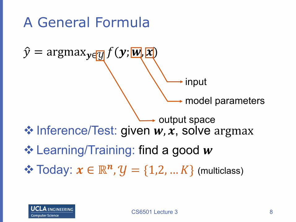
𝑦0 = argmax𝒚∈𝒴 𝑓(𝒚;𝒘, 𝒙)

v Inference/Test: given 𝒘, 𝒙, solve argmaxv Learning/Training: find a good 𝒘vToday: 𝒙 ∈ ℝ𝒏,𝒴 = {1,2, …𝐾} (multiclass)

CS6501 Lecture 3 8

input

output space

model parameters

This Lecture




CS6501 Lecture 3 9

One against all strategy

CS6501 Lecture 3 10

One against All learning

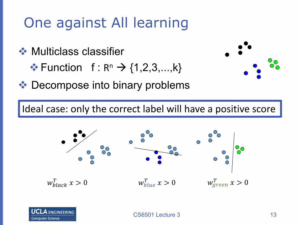
v Multiclass classifiervFunction f : Rn à {1,2,3,...,k}

v Decompose into binary problems

CS6501 Lecture 3 11

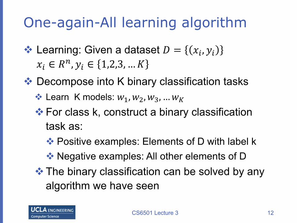
One-again-All learning algorithm

v Learning: Given a dataset 𝐷 = 𝑥C, 𝑦C𝑥C ∈ 𝑅E, 𝑦C ∈ 1,2,3, …𝐾

v Decompose into K binary classification tasksv Learn K models: 𝑤F,𝑤G, 𝑤H, …𝑤IvFor class k, construct a binary classification

task as: v Positive examples: Elements of D with label k v Negative examples: All other elements of D

vThe binary classification can be solved by any algorithm we have seen

CS6501 Lecture 3 12

One against All learning



𝑤JKLMN& 𝑥 > 0 𝑤JKRS& 𝑥 > 0 𝑤TUSSE& 𝑥 > 0

Idealcase:onlythecorrectlabelwillhaveapositivescore

CS6501 Lecture 3 13

One-again-All Inference


v Decompose into K binary classification tasksv Learn K models: 𝑤F,𝑤G, 𝑤H, …𝑤I

v Inference: “Winner takes all”v 𝑦0 = argmaxV∈{F,G,…I}𝑤V&𝑥

v An instance of the general form𝑦0 = argmax𝒚∈𝒴 𝑓(𝒚;𝒘, 𝒙)

CS6501 Lecture 3 14

Forexample:y = argmax(𝑤JKLMN& 𝑥, 𝑤JKRS& 𝑥, 𝑤TUSSE& 𝑥)

𝑤 = {𝑤F, 𝑤G, …𝑤I},𝑓 𝒚;𝒘, 𝒙 = 𝒘V&𝑥

One-again-All analysis

v Not always possible to learn v Assumption: each class individually separable from

all the others

v No theoretical justification vNeed to make sure the range of all classifiers is

the same – we are comparing scores produced by K classifiers trained independently.

v Easy to implement; work well in practice

CS6501 Lecture 3 15

One v.s. One (All against All) strategy

CS6501 Lecture 3 16



Training

One v.s. One learning

Test

CS6501 Lecture 3 17

One-v.s-One learning algorithm


v Decompose into C(K,2) binary classification tasksv Learn C(K,2) models: 𝑤F,𝑤G, 𝑤H, …𝑤I∗(IYF)/GvFor each class pair (i,j), construct a binary

classification task as: v Positive examples: Elements of D with label iv Negative examples Elements of D with label jv The binary classification can be solved by any

algorithm we have seen

CS6501 Lecture 3 18

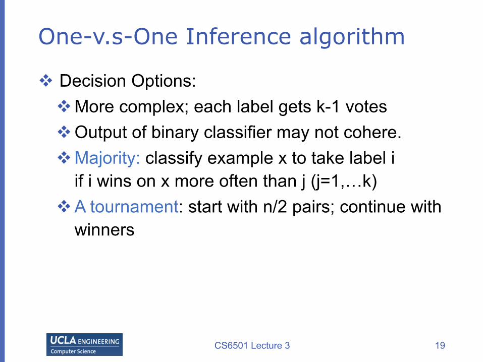
One-v.s-One Inference algorithm

v Decision Options: vMore complex; each label gets k-1 votesvOutput of binary classifier may not cohere. vMajority: classify example x to take label i

if i wins on x more often than j (j=1,…k) vA tournament: start with n/2 pairs; continue with

winners

CS6501 Lecture 3 19

Classifying with One-vs-one

Tournament

1red,2yellow,2greenè ?

MajorityVote

All are post-learning and might cause weird stuff

CS6501 Lecture 3 20

One-v.s.-one Assumption

vEvery pair of classes is separable

CS6501 Lecture 3

21

ItispossibletoseparateallkclasseswiththeO(k2)classifiers

Decision Regions

Comparisons

v One against allv O(K) weight vectors to train and storev Training set of the binary classifiers may unbalancedv Less expressive; make a strong assumption

v One v.s. One (All v.s. All)v O(𝐾G) weight vectors to train and storev Size of training set for a pair of labels could be small ⇒ overfitting of the binary classifiers

v Need large space to store model

CS6501 Lecture 3 22

Problems with Decompositions

v Learning optimizes over local metricsvDoes not guarantee good global performancevWe don’t care about the performance of the

local classifiersv Poor decomposition Þ poor performance

vDifficult local problemsv Irrelevant local problems

v Efficiency: e.g., All vs. All vs. One vs. Allv Not clear how to generalize multi-class to

problems with a very large # of output

CS6501 Lecture 3 23

Still an ongoing research direction

Key questions:v How to deal with large number of classesv How to select “right samples” to train binary classifiers

v Error-correcting tournaments[Beygelzimer, Langford, Ravikumar 09]

v Logarithmic Time One-Against-Some [Daume, Karampatziakis, Langford, Mineiro 16]

v Label embedding trees for large multi-class tasks.[Bengio, Weston, Grangier 10]

v …

CS6501 Lecture 3 24

Decomposition methods: Summary

vGeneral Ideas:v Decompose the multiclass problem into many

binary problemsv Prediction depends on the decomposition

v Constructs the multiclass label from the output of the binary classifiers

v Learning optimizes local correctnessv Each binary classifier don’t need to be globally

correct and isn’t aware of the prediction procedure

CS6501 Lecture 3 25

This Lecture




CS6501 Lecture 3 26

Revisit One-again-All learning algorithm


v Decompose into K binary classification tasksv Learn K models: 𝑤F,𝑤G, 𝑤H, …𝑤Iv 𝑤N:separate class 𝑘 from others

v Prediction𝑦0 = argmaxV∈{F,G,…I}𝑤V&𝑥

CS6501 Lecture 3 27

Observation

v At training time, we require 𝑤C&𝑥to be positive for examples of class 𝑖.

v Really, all we need is for 𝑤C&𝑥 to be more than all others ⇒ this is a weaker requirement

CS6501 Lecture 3 28

Forexampleswithlabel𝑖,weneed𝑤C&𝑥 > 𝑤_&𝑥 forall𝑗

Perceptron-style algorithm

vFor each training example 𝑥, 𝑦v If for some y’, 𝑤V&𝑥 ≤ 𝑤Vb& 𝑥 mistake!

v 𝑤V ← 𝑤V + 𝜂𝑥 update to promote yv 𝑤Vb ← 𝑤Vb − 𝜂𝑥 update to demote y’

CS6501 Lecture 3 29

Forexampleswithlabel𝑖,weneed𝑤C&𝑥 > 𝑤_&𝑥 forall𝑗

Whyadd𝜂𝑥 to𝑤Vpromotelabel𝑦:Beforeupdates y =< 𝑤ViKj, 𝑥 >Afterupdates y =< 𝑤VESk, 𝑥 >=< 𝑤ViKj +𝜂𝑥, 𝑥 >

=< 𝑤ViKj, 𝑥 > +𝜂 < 𝑥, 𝑥 >Note!< 𝑥, 𝑥 >= 𝑥& 𝑥 > 0

A Perceptron-style Algorithm

Prediction: argmaxq𝑤V&𝑥

CS6501 Lecture 3 30

Initialize𝒘 ← 𝟎 ∈ ℝEFor epoch 1…𝑇:For (𝒙,𝑦) in 𝒟:For 𝑦b ≠ 𝑦if𝑤V&𝑥 < 𝑤Vb& 𝑥 make a mistake𝑤V ← 𝑤V + 𝜂𝑥promote y𝑤Vb ← 𝑤Vb − 𝜂𝑥 demote y’

Return 𝒘

Given a training set 𝒟 = { 𝒙,𝑦 }

Howtoanalyzethisalgorithmandsimplifytheupdaterules?

Linear Separability with multiple classes

v Let’s rewrite the equation𝑤C&𝑥 > 𝑤_&𝑥 for all 𝑗

v Instead of having 𝑤F,𝑤G, 𝑤H, …𝑤I, we want to represent the model using a single vector 𝑤

𝑤& > 𝑤& for all j

vHow?

CS6501 Lecture 3 31

ChangetheinputrepresentationLet’sdefine𝜙(𝑥, 𝑦),suchthat𝑤&𝜙 𝑥, 𝑖 > 𝑤&𝜙 𝑥, 𝑗 ∀𝑗

? ?

multiplemodelsv.s.multipledatapoints

Kesler construction

CS6501 Lecture 3 32

𝑤C&𝑥 > 𝑤_&𝑥∀j

vmodels:𝑤F,𝑤G, …𝑤I, 𝑤N ∈ 𝑅E

v Input:𝑥 ∈ 𝑅E

𝑤&𝜙 𝑥, 𝑖 > 𝑤&𝜙 𝑥, 𝑗 ∀𝑗

Assumewehaveamulti-classproblemwithKclassandnfeatures.

Kesler construction

CS6501 Lecture 3 33

𝑤C&𝑥 > 𝑤_&𝑥∀j




vOnly one model:𝑤 ∈ 𝑅E×I


Kesler construction

CS6501 Lecture 3 34

𝑤C&𝑥 > 𝑤_&𝑥∀𝑗




v Only one model:𝑤 ∈ 𝑅EI

v Define 𝜙 𝑥, 𝑦 for label ybeing associated to input x

𝜙 𝑥, 𝑦 =

0E⋮𝑥⋮0E EI×F


𝑥in𝑦}~ block;Zeros elsewhere

Kesler construction

CS6501 Lecture 3 35

𝑤C&𝑥 > 𝑤C&𝑥∀iv models:

𝑤F,𝑤G,…𝑤I,𝑤N ∈ 𝑅E



𝑤 =

𝑤F⋮𝑤V⋮𝑤E EI×F

𝜙 𝑥, 𝑦 =


𝑤&𝜙 𝑥, 𝑦 = 𝑤V&𝑥



Kesler construction

CS6501 Lecture 3 36

𝑤&𝜙 𝑥, 𝑖 > 𝑤&𝜙 𝑥, 𝑗 ∀𝑗⇒ 𝑤& 𝜙 𝑥, 𝑖 − 𝜙 𝑥, 𝑗 > 0∀𝑗

𝑤 =


[𝜙 𝑥, 𝑖 − 𝜙 𝑥, 𝑗 ] =

0E⋮𝑥⋮−𝑥⋮0E EI×F

𝑥in𝑖}~ block;


−𝑥in𝑗}~ block;

binaryclassificationproblem

Linear Separability with multiple classes

CS6501 Lecture 3 37

Whatwewant𝑤&𝜙 𝑥, 𝑖 > 𝑤&𝜙 𝑥, 𝑗 ∀𝑗⇒ 𝑤& 𝜙 𝑥, 𝑖 − 𝜙 𝑥, 𝑗 > 0∀𝑗

Forallexample(x,y)withallotherlabelsy’indataset,𝑤 innK dimensionshouldlinearlyseparate𝜙 𝑥, 𝑖 − 𝜙 𝑥, 𝑗 and−[𝜙 𝑥, 𝑖 − 𝜙 𝑥, 𝑗 ]

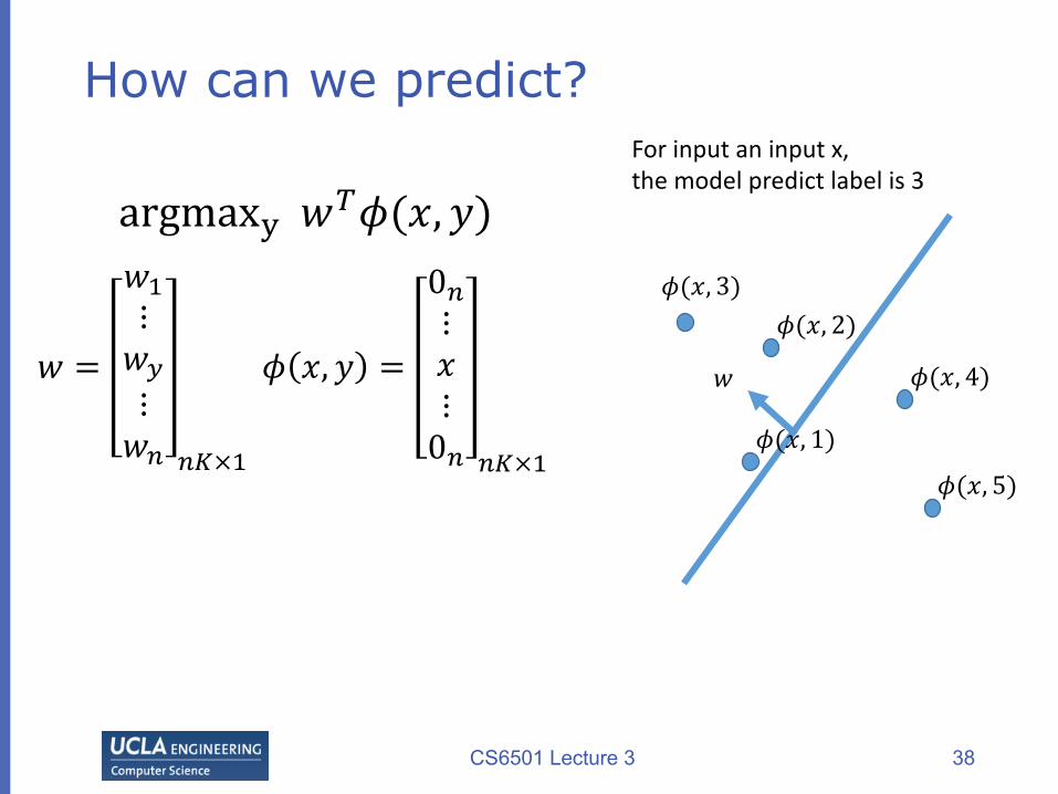
How can we predict?

CS6501 Lecture 3 38

argmaxq𝑤&𝜙(𝑥, 𝑦)

𝑤 =


𝜙 𝑥, 𝑦 =


𝑤

𝜙(𝑥, 3)

Forinputaninputx,themodelpredictlabelis3

𝜙(𝑥, 2)

𝜙(𝑥, 1)

𝜙(𝑥, 4)

𝜙(𝑥, 5)

How can we predict?

CS6501 Lecture 3 39


𝑤 =


𝜙 𝑥, 𝑦 =


𝑤𝜙(𝑥, 3)

Forinputaninputx,themodelpredictlabelis3

𝜙(𝑥, 2)

𝜙(𝑥, 1)

𝜙(𝑥, 4)

𝜙(𝑥, 5)

ThisisequivalenttoargmaxV∈{F,G,…I}𝑤V&𝑥

Constraint Classification

vGoal:vTraining:

vFor each example 𝑥, 𝑖v Update model if 𝑤& 𝜙 𝑥, 𝑖 − 𝜙 𝑥, 𝑗 < 0, ∀𝑗

CS6501 Lecture 3 40

𝑤 𝜙 𝑥, 𝑖 − 𝜙 𝑥, 𝑗 ≥ 0∀𝑗

-xx

Transform Examples

2>12>32>4

2>1

2>3

2>4


Prediction: argmaxq𝑤&𝜙(𝑥, 𝑦)

CS6501 Lecture 3 41

Initialize𝒘 ← 𝟎 ∈ ℝE

For epoch 1…𝑇:For (𝒙,𝑦) in 𝒟:For 𝑦b ≠ 𝑦if𝑤& 𝜙 𝑥, 𝑦 − 𝜙 𝑥, 𝑦′ < 0𝒘 ←𝒘+𝜂 𝜙 𝑥, 𝑦 − 𝜙 𝑥, 𝑦′

Return 𝒘


Howtointerpretthisupdaterule?

Thisneeds 𝐷 ×𝐾 updates,doweneedallofthem?

An alternative training algorithm

vGoal:

vTraining:vFor each example 𝑥, 𝑖

v Find the prediction of the current model:𝑦0 = argmax�𝑤&𝜙(𝑥, 𝑗)

v Update model if 𝑤& 𝜙 𝑥, 𝑖 − 𝜙 𝑥, 𝑦0 < 0, ∀𝑦′

CS6501 Lecture 3 42

𝑤 𝜙 𝑥, 𝑖 − 𝜙 𝑥, 𝑗 ≥ 0∀𝑗⇒ 𝑤&𝜙 𝑥, 𝑖 − max

_�C𝑤&𝜙 𝑥, 𝑖 ≥ 0

⇒ 𝑤&𝜙 𝑥, 𝑖 − max_

𝑤&𝜙 𝑥, 𝑖 ≥ 0



CS6501 Lecture 3 43


For epoch 1…𝑇:For (𝒙,𝑦) in 𝒟:

�̂� = argmaxqb𝑤&𝜙(𝑥, 𝑦′) if𝑤& 𝜙 𝑥, 𝑦 − 𝜙 𝑥, 𝑦0 < 0

𝒘←𝒘+𝜂 𝜙 𝑥, 𝑦 − 𝜙 𝑥, 𝑦�Return 𝒘





CS6501 Lecture 3 44



�̂� = argmaxqb𝑤&𝜙(𝑥, 𝑦′) if𝑤& 𝜙 𝑥, 𝑦 − 𝜙 𝑥, 𝑦0 < 0𝒘 ←𝒘+𝜂 𝜙 𝑥, 𝑦 − 𝜙 𝑥, 𝑦0

Return 𝒘



Thereareonlytwosituations:1.𝑦0 = 𝑦:𝜙 𝑥, 𝑦 − 𝜙 𝑥, 𝑦0 =02.𝑤& 𝜙 𝑥, 𝑦 − 𝜙 𝑥, 𝑦0 < 0



CS6501 Lecture 3 45



�̂� = argmaxqb𝑤&𝜙(𝑥, 𝑦′) 𝒘 ←𝒘+𝜂 𝜙 𝑥, 𝑦 − 𝜙 𝑥, 𝑦0

Return 𝒘



Consider multiclass margin

CS6501 Lecture 3 46

Marginal constraint classifier

vGoal: for every (x,y) in the training data set

CS6501 Lecture 3 47

minV��V

𝑤& 𝜙 𝑥, 𝑦 − 𝜙 𝑥, 𝑦′ ≥ 𝛿

⇒ 𝑤&𝜙 𝑥, 𝑦 − maxV�Vb

𝑤&𝜙 𝑥, 𝑦′ ≥ 𝛿

⇒ 𝑤&𝜙 𝑥, 𝑖 − [maxV�Vb

𝑤&𝜙 𝑥, 𝑗 + 𝛿] ≥ 0

𝛿 𝛿𝛿

Constraintsviolated⇒ needanupdate

Let’sdefine:

Δ 𝑦, 𝑦b = � 𝛿if𝑦 ≠ 𝑦′0𝑖𝑓𝑦 = 𝑦′

Checkif𝑦 = 𝑎𝑟𝑔𝑚𝑎𝑥V�𝑤&𝜙 𝑥, 𝑦′ + Δ(𝑦, 𝑦b)



CS6501 Lecture 3 48



�̂� = argmaxqb𝑤&𝜙 𝑥, 𝑦′ + Δ(𝑦, y’) 𝒘 ←𝒘+𝜂 𝜙 𝑥, 𝑦 − 𝜙 𝑥, 𝑦0

Return 𝒘



𝛿 𝛿𝛿

Remarks

v This approach can be generalized to train a ranker; in fact, any output structurev We have preference over label assignmentsv E.g., rank search results, rank movies / products

CS6501 Lecture 3 49

A peek of a generalized Perceptron model


CS6501 Lecture 3 50



�̂� = argmaxqb𝑤&𝜙(𝑥, 𝑦′) + Δ(𝑦, y’) 𝒘 ←𝒘+𝜂 𝜙 𝑥, 𝑦 − 𝜙 𝑥, 𝑦0

Return 𝒘


Structuralprediction/Inference

Modelupdate

Structuredoutput

Structuralloss

Recap: A Perceptron-style Algorithm

Prediction: argmaxq𝑤V&𝑥

CS6501 Lecture 3 51

Initialize𝒘 ← 𝟎 ∈ ℝEFor epoch 1…𝑇:For (𝒙,𝑦) in 𝒟:For 𝑦b ≠ 𝑦if𝑤V&𝑥 < 𝑤Vb& 𝑥 make a mistake𝑤V ← 𝑤V + 𝜂𝑥promote y𝑤Vb ← 𝑤Vb − 𝜂𝑥 demote y’

Return 𝒘


Recap: Kesler construction

CS6501 Lecture 3 52

𝑤C&𝑥 > 𝑤C&𝑥∀iv models:

𝑤F,𝑤G,…𝑤I,𝑤N ∈ 𝑅E



𝑤 =


𝜙 𝑥, 𝑦 =


𝑤&𝜙 𝑥, 𝑦 = 𝑤V&𝑥



Geometric interpretation

CS6501 Lecture 3 53


𝑤𝜙(𝑥, 3)

#features=n;#classes=K

𝜙(𝑥, 2)

𝜙(𝑥, 1)

𝜙(𝑥, 4)

𝜙(𝑥, 5)

argmaxV∈{F,G,…I}𝑤V&𝑥

In 𝑅�I spaceIn 𝑅� space

𝑤G𝑤F

𝑤H

𝑤

𝑤¡

Recap: A Perceptron-style Algorithm


CS6501 Lecture 3 54



�̂� = argmaxqb𝑤&𝜙(𝑥, 𝑦′) 𝒘 ←𝒘+𝜂 𝜙 𝑥, 𝑦 − 𝜙 𝑥, 𝑦0

Return 𝒘



Multi-category to Constraint Classification

v Multiclassv (x, A) Þ (x, (A>B, A>C, A>D) )

v Multilabelv (x, (A, B))Þ (x, ( (A>C, A>D, B>C, B>D) )

v Label Rankingv (x, (5>4>3>2>1)) Þ (x, ( (5>4, 4>3, 3>2, 2>1) )

CS6501 Lecture 3 55

Generalized constraint classifiers

v In all cases, we have examples (x,y) with y Î Skv Where Sk : partial order over class labels {1,...,k}

v defines “preference” relation ( > ) for class labelingv Consequently, the Constraint Classifier is: h: X® Sk

v h(x) is a partial orderv h(x) is consistent with y if (i<j) Î y è (i<j) Îh(x)

CS6501 Lecture 3 56

Justlikeinthemulticlasswelearnonewi Î Rn foreachlabel,thesameisdoneformulti-labelandranking.TheweightvectorsareupdatedaccordingwiththerequirementsfromyÎ Sk

Multi-category to Constraint Classification

Solving structured prediction problems by ranking algorithmsv Multiclass

v (x, A) Þ (x, (A>B, A>C, A>D) )v Multilabel

v (x, (A, B))Þ (x, ( (A>C, A>D, B>C, B>D) ) v Label Ranking

v (x, (5>4>3>2>1)) Þ (x, ( (5>4, 4>3, 3>2, 2>1) )yÎ Sk h:X® Sk

CS6501 Lecture 3 57

Properties of Construction (Zimak et. al 2002, 2003)

v Can learn any argmax wi.x function (even when i isn’t linearly separable from the union of the others)

v Can use any algorithm to find linear separationv Perceptron Algorithm

v ultraconservative online algorithm [Crammer, Singer 2001]

v Winnow Algorithmv multiclass winnow [ Masterharm 2000 ]

v Defines a multiclass margin by binary margin in RKN

v multiclass SVM [Crammer, Singer 2001]

CS6501 Lecture 3 58

This Lecture




CS6501 Lecture 3 59

Recall: Margin for binary classifiers

vThe margin of a hyperplane for a dataset is the distance between the hyperplane and the data point nearest to it.

60

++

++

+ +++

-- --

-- -- --

---- --

--

Marginwithrespecttothishyperplane

CS6501 Lecture 3

Multi-class SVM

v In a risk minimization frameworkvGoal: D = x£, y£ C¤F

�

1. 𝑤V¦& 𝑥C > 𝑤Vb& 𝑥C for all 𝑖, y’

2. Maximizing the margin

CS6501 Lecture 3 61

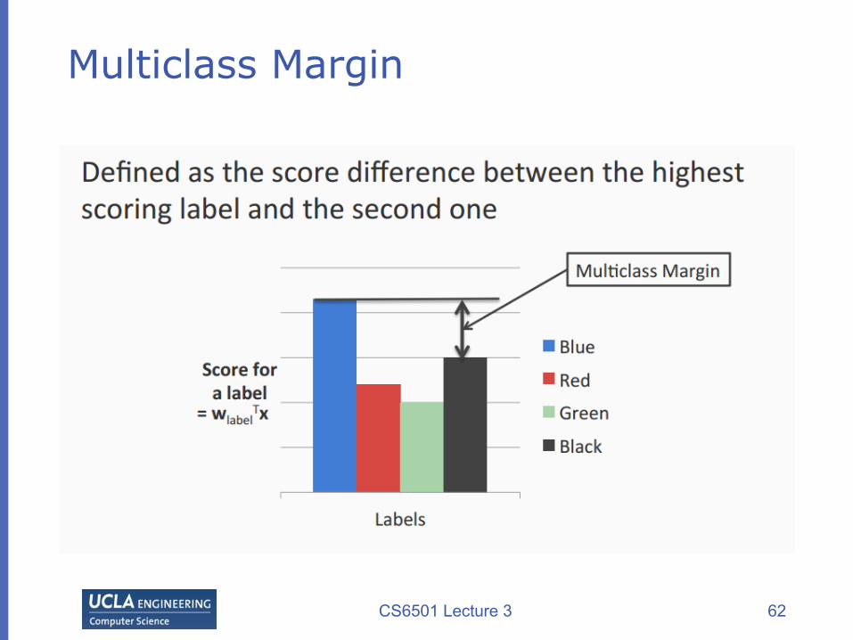
Multiclass Margin

62CS6501 Lecture 3

Multiclass SVM (Intuition)

v Binary SVMv Maximize margin. Equivalently,

Minimize norm of weights such that the closest points to the hyperplane have a score 1

v Multiclass SVMv Each label has a different weight vector

(like one-vs-all)v Maximize multiclass margin. Equivalently,

Minimize total norm of the weights such that the true label is scored at least 1 more than the second best one

63CS6501 Lecture 3

Multiclass SVM in the separable case

64

RecallhardbinarySVM

Thescoreforthetruelabelishigherthanthescoreforany otherlabelby1

Sizeoftheweights.Effectively,regularizer

CS6501 Lecture 3

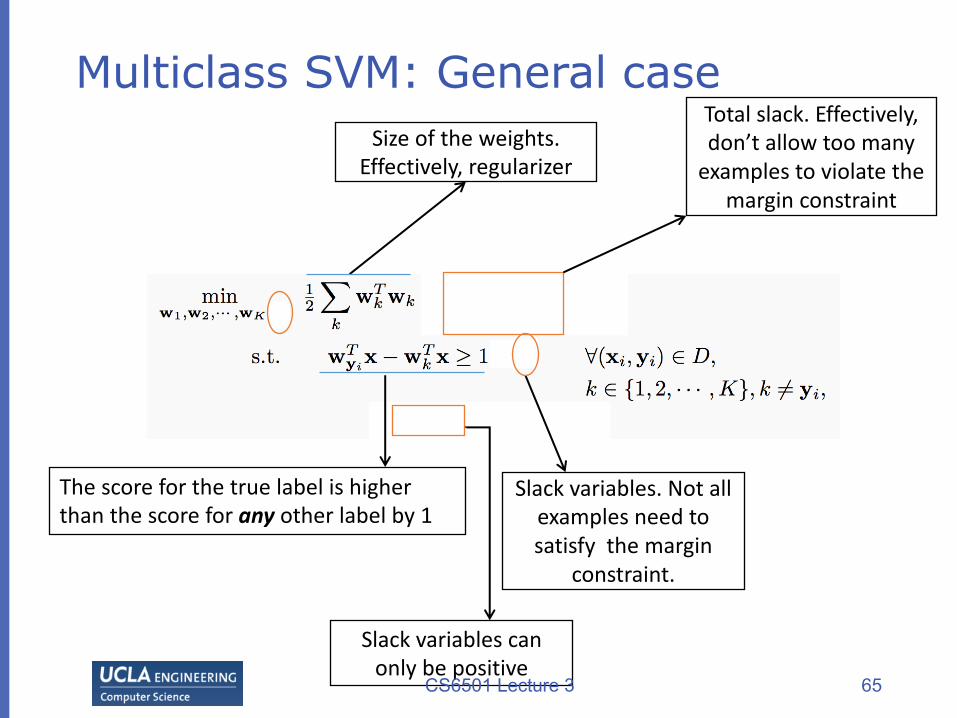
Multiclass SVM: General case

65


Thescoreforthetruelabelishigherthanthescoreforany otherlabelby1

Slackvariables.Notallexamplesneedtosatisfythemargin

constraint.

Totalslack.Effectively,don’tallowtoomanyexamplestoviolatethe

marginconstraint

Slackvariablescanonlybepositive

CS6501 Lecture 3

Multiclass SVM: General case

66

Thescoreforthetruelabelishigherthanthescoreforany otherlabelby1- »i


Slackvariables.Notallexamplesneedtosatisfythemargin

constraint.

Totalslack.Effectively,don’tallowtoomanyexamplestoviolatethe

marginconstraint

Slackvariablescanonlybepositive

CS6501 Lecture 3

Recap: An alternative SVM formulation

min𝒘,J,𝝃

FG𝒘&𝒘 + 𝐶 ∑ 𝜉C�

C

s. ty£(𝐰𝐱£ + 𝑏) ≥ 1 − 𝜉C;𝜉C ≥ 0∀𝑖vRewrite the constraints:

𝜉C ≥ 1 −y£(𝐰𝐱£ + 𝑏);𝜉C ≥ 0 ∀𝑖v In the optimum, 𝜉C = max(0, 1 −y£(𝐰𝐱£ + 𝑏))

vSoft SVM can be rewritten as:min𝒘,J

FG𝒘&𝒘 + 𝐶 ∑ max(0, 1 −y£(𝐰𝐱£ + 𝑏))�

C

CS6501 Lecture 3 67

EmpiricallossRegularizationterm

Rewrite it as unconstraint problem

mink

FG∑ 𝑤N&�

N 𝑤N + 𝐶∑ (maxN

Δ 𝑦C, 𝑘 + 𝑤N&𝑥 − 𝑤V¦& 𝑥)�

C

CS6501 Lecture 3 68

Let’sdefine:

Δ 𝑦, 𝑦b = � 𝛿if𝑦 ≠ 𝑦′0𝑖𝑓𝑦 = 𝑦′

Multiclass SVM

v Generalizes binary SVM algorithmv If we have only two classes, this reduces to the

binary (up to scale)

v Comes with similar generalization guarantees as the binary SVM

v Can be trained using different optimization methodsv Stochastic sub-gradient descent can be generalized

69CS6501 Lecture 3

Exercise!

v Write down SGD for multiclass SVM

v Write down multiclas SVM with Keslerconstruction

CS6501 Lecture 3 70

This Lecture




CS6501 Lecture 3 71

Recall: (binary) logistic regression

min𝒘12𝒘

&𝒘 + 𝐶°log( 1 + 𝑒Yq²(𝐰³𝐱²))�

C

Assume labels are generated using the following probability distribution:

CS6501 Lecture 3 72

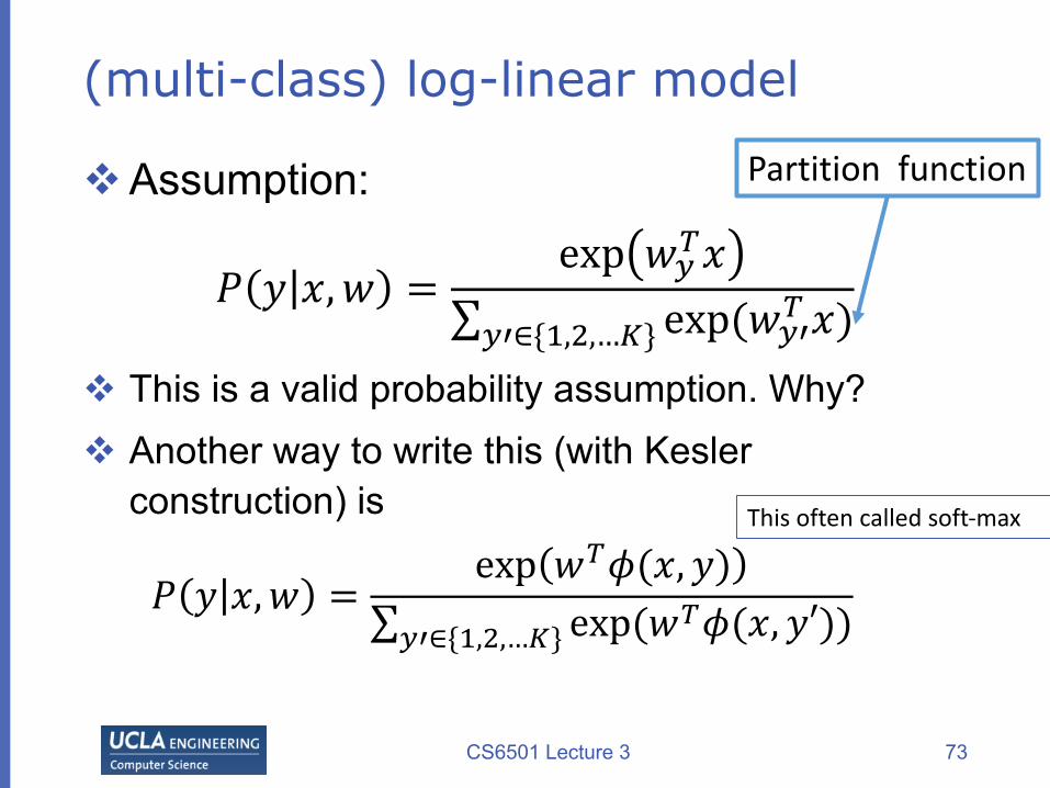
(multi-class) log-linear model

vAssumption:

𝑃 𝑦 𝑥, 𝑤 =exp 𝑤V&𝑥

∑ exp(𝑤Vb& 𝑥)�Vb∈{F,G,…I}

v This is a valid probability assumption. Why?v Another way to write this (with Kesler

construction) is

𝑃 𝑦 𝑥,𝑤 =exp 𝑤&𝜙(𝑥, 𝑦)

∑ exp(𝑤&𝜙(𝑥, 𝑦′))�Vb∈{F,G,…I}

CS6501 Lecture 3 73

Thisoftencalledsoft-max

Partitionfunction

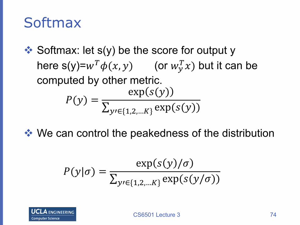
Softmax

v Softmax: let s(y) be the score for output yhere s(y)=𝑤&𝜙(𝑥, 𝑦) (or 𝑤V&𝑥) but it can be computed by other metric.

v We can control the peakedness of the distribution

CS6501 Lecture 3 74

𝑃(𝑦) =exp 𝑠(𝑦)

∑ exp(𝑠(𝑦))�Vb∈{F,G,…I}

𝑃(𝑦|𝜎) =exp 𝑠 𝑦 /𝜎

∑ exp(𝑠(𝑦/𝜎))�Vb∈{F,G,…I}

Example

CS6501 Lecture 3 75

-0.4

-0.2

0

0.2

0.4

0.6

0.8

1

1.2

Dog Cat Mouse Duck

S(dog)=.5;s(cat)=1;s(mouse)=0.3;s(duck)=-0.2

score softmax (hard)max(𝜎→0)

softmax(𝜎=0.5) softmax(𝜎=2)

Log linear model

𝑃 𝑦 𝑥,𝑤 = ·¸¹ kº»¼∑ ·¸¹(kº�» ¼)�º�∈{½,¾,…¿}

log 𝑃 𝑦 𝑥,𝑤 = log(exp 𝑤V&𝑥 ) − log(∑ exp(𝑤V�& 𝑥))�

Vb∈{F,G,…I}

= 𝑤V&𝑥 − log(∑ exp(𝑤V�& 𝑥))�

Vb∈{F,G,…I}

Note:

CS6501 Lecture 3 76

Linearfunction Exceptthisterm

Maximum log-likelihood estimation

v Training can be done by maximum log-likelihood estimation i.e. max

klog 𝑃(𝐷 𝑤

D={(𝑥C, 𝑦C)}

𝑃(𝐷 𝑤 = ΠC·¸¹ kº¦

» ¼¦∑ ·¸¹(kº�

» ¼¦)�º�∈{½,¾,…¿}

log 𝑃(𝐷 𝑤 = ∑ [𝑤V¦& 𝑥C −�

C log∑ exp(𝑤V�& 𝑥C)�

Vb∈{F,G,…I} ]

CS6501 Lecture 3 77

Maximum a posteriori

D={(𝑥C, 𝑦C)}

𝑃 𝑤 𝐷 ∝ 𝑃 𝑤 𝑃 𝐷 𝑤

m𝑎𝑥k −FG ∑ 𝑤V&𝑤V +�

V 𝐶 ∑ [𝑤V¦& 𝑥C −�

C log∑ exp(𝑤V�& 𝑥C)�

Vb∈{F,G,…I} ]

or

minkFG∑ 𝑤V&𝑤V +�

V 𝐶 ∑ [�C log∑ exp 𝑤V�& 𝑥C − 𝑤V¦

& 𝑥C�Vb∈{F,G,…I} ]

CS6501 Lecture 3 78

CanyouuseKesler constructiontorewritethisformulation?

Comparisonsv Multi-class SVM:

mink

FG∑ 𝑤N&�

N 𝑤N + 𝐶 ∑ (maxN(Δ 𝑦C, 𝑘 + 𝑤N&𝑥 − 𝑤V¦

& 𝑥))�C

v Log-linear model w/ MAP (multi-class)mink

F

G∑ 𝑤N&𝑤N + 𝐶�N ∑ [�C log∑ exp 𝑤N&𝑥C − 𝑤V¦

& 𝑥C�N∈{F,G,…I} ]

v Binary SVM:

min𝒘FG𝒘&𝒘 + 𝐶 ∑ max(0, 1 −y£(𝐰𝐱£))�

C

v Log-linear mode (logistic regression)

min𝒘FG𝒘&𝒘 + 𝐶 ∑ log( 1 + 𝑒Yq²(𝐰³𝐱²))�

C

CS6501 Lecture 3 79

lecture 3: multi-class classification · previous lecture vbinary linear classification models...

Documents