sp’10bafna/ideker classification (svms / kernel method)

Sp’10 Bafna/Ideker

Classification (SVMs / Kernel method)


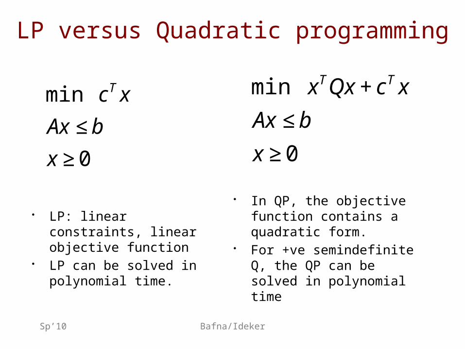
LP versus Quadratic programming

€

min cT x

Ax ≤ b

x ≥ 0

€

min xTQx + cT x

Ax ≤ b

x ≥ 0

• LP: linear constraints, linear objective function

• LP can be solved in polynomial time.

• In QP, the objective function contains a quadratic form.

• For +ve semindefinite Q, the QP can be solved in polynomial time


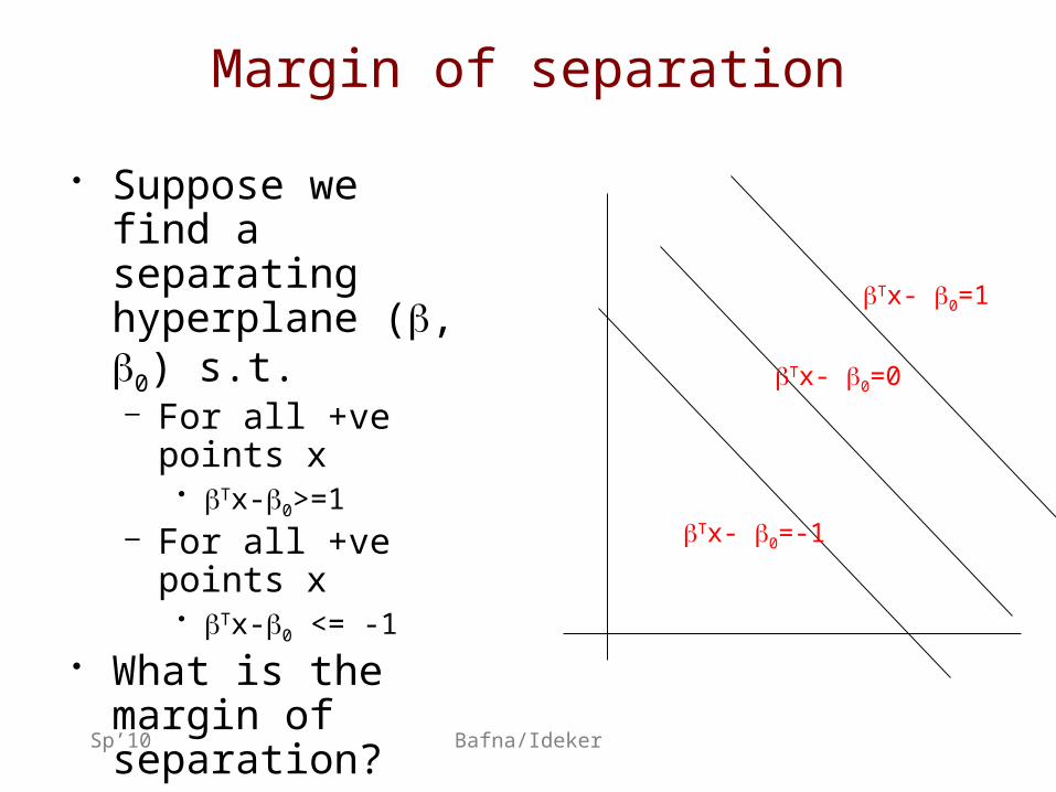
Margin of separation

• Suppose we find a separating hyperplane (, 0) s.t.– For all +ve points

x• Tx-0>=1

– For all +ve points x• Tx-0 <= -1

• What is the margin of separation?

Tx- 0=0

Tx- 0=1

Tx- 0=-1


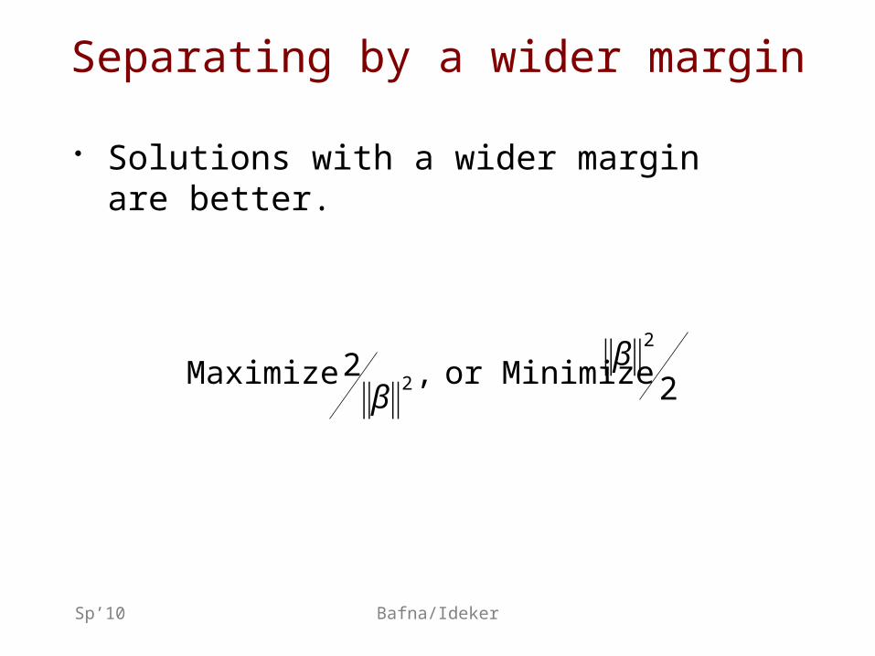
Separating by a wider margin

• Solutions with a wider margin are better.

€

Maximize 2β

2 , or Minimize β

2

2


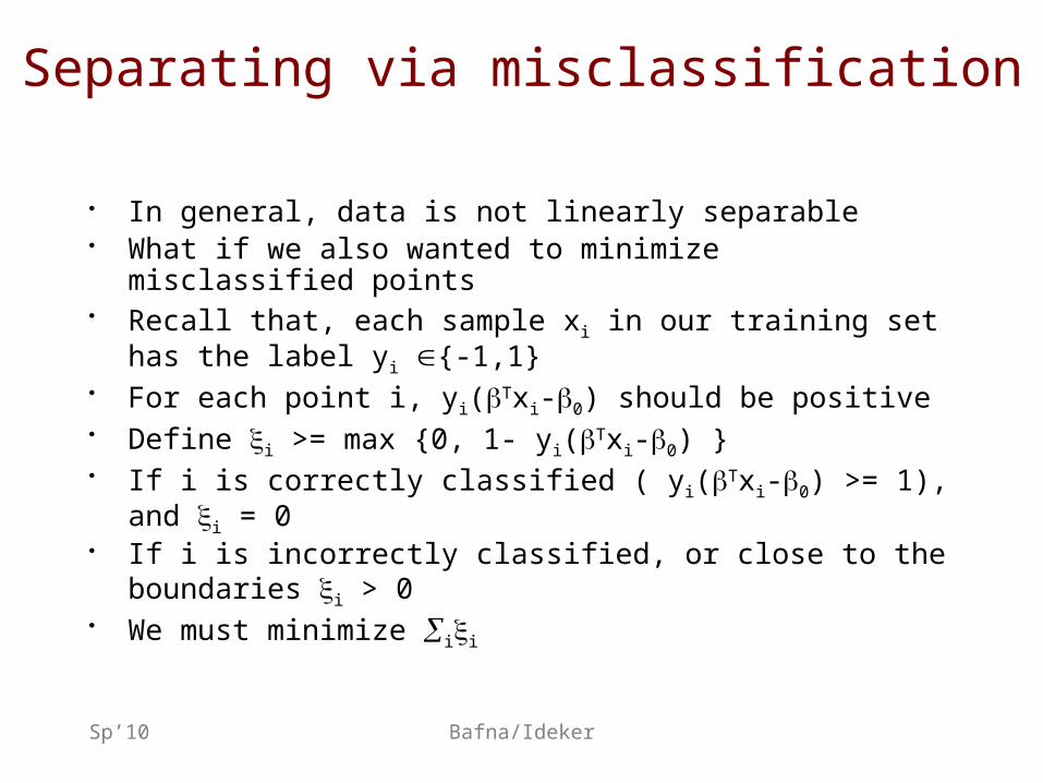
Separating via misclassification

• In general, data is not linearly separable• What if we also wanted to minimize misclassified points• Recall that, each sample xi in our training set has the

label yi {-1,1} • For each point i, yi(Txi-0) should be positive• Define i >= max {0, 1- yi(Txi-0) }• If i is correctly classified ( yi(Txi-0) >= 1), and i = 0• If i is incorrectly classified, or close to the boundaries i

> 0• We must minimize ii


Support Vector machines (wide margin and misclassification)

• Maximimize margin while minimizing misclassification

• Solved using non-linear optimization techniques

• The problem can be reformulated to exclusively using cross products of variables, which allows us to employ the kernel method.

• This gives a lot of power to the method. €

minβ

2

2 +C ξ ii∑


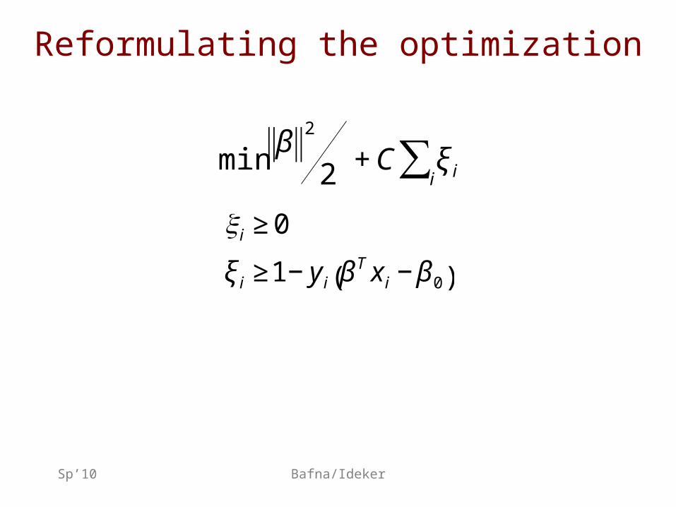
Reformulating the optimization

€

minβ

2

2 +C ξ ii∑

€

ξ i ≥ 0

ξ i ≥1− y i βT x i −β 0( )


Lagrangian relaxation

€

L =β

2

2+C ξ ii

∑ − α ii∑ ξ i −1+ y i β

T x i −β 0( )( ) − λ ii∑ ξ i

• Goal

• S.t.

• We minimize€

minβ

2

2+C ξ ii

∑

€

ξ i ≥ 0

ξ i ≥1− y i βT x i −β 0( )


Simplifying

€

L =β

2

2+C ξ ii

∑ − α ii∑ ξ i −1+ y i β

T x i −β 0( )( ) − λ ii∑ ξ i

= β Tβ

2− α iy ix ii∑

⎛

⎝ ⎜

⎞

⎠ ⎟+ C −α i − λ i( )

i∑ ξ i + α ii

∑ y iβ 0 + α ii∑

• For fixed >= 0, >= 0, we minimize the lagrangian

€

∂L∂β

= β − y ii∑ α ix i = 0 (1)

∂L

∂β 0

= y ii∑ α i = 0 (2)

∂L

∂ξ i=C −α i − λ i = 0 (3)


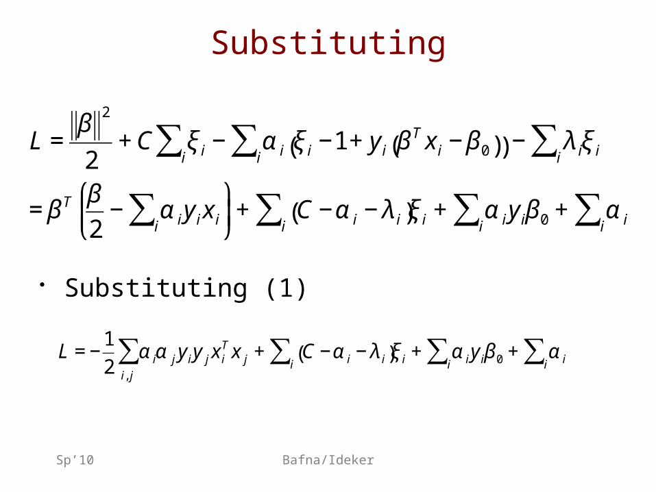
Substituting

• Substituting (1)

€

L =β

2

2+C ξ ii

∑ − α ii∑ ξ i −1+ y i β

T x i −β 0( )( ) − λ ii∑ ξ i

= β Tβ

2− α iy ix ii∑

⎛

⎝ ⎜

⎞

⎠ ⎟+ C −α i − λ i( )

i∑ ξ i + α ii

∑ y iβ 0 + α ii∑

€

L = −1

2α iα jy iy jx i

T x ji, j

∑ + C −α i − λ i( )i

∑ ξ i + α ii∑ y iβ 0 + α ii

∑


• Substituting (2,3), we have the minimization problem€

L = −1

2α iα jy iy jx i

T x ji, j

∑ + C −α i − λ i( )i

∑ ξ i + α ii∑ y iβ 0 + α ii

∑

€

min −1

2α iα jy iy jx i

T x ji, j

∑ + α ii∑

s.t.

y iα ii∑ = 0

0 ≤ α i ≤ C


Classification using SVMs

• Under these conditions, the problem is a quadratic programming problem and can be solved using known techniques

• Quiz: When we have solved this QP, how do we classify a point x?

€

f (x) = β T x −β 0 = y ii∑ α ix i

T x −β 0


The kernel method

• The SVM formulation can be solved using QP on dot-products.

• As these are wide-margin classifiers, they provide a more robust solution.

• However, the true power of SVMs approach from using ‘the kernel method’, which allows us to go to higher dimensional (and non-linear spaces)


kernel

• Let X be the set of objects – Ex: X =the set of samples in micro-arrays.– Each object xX is a vector of gene

expression values• k: X X -> R is a positive semidefinite

kernel if– k is symmetric.– k is +ve semidefinite

€

k(x,x ') = k(x',x)

€

cT kc ≥ 0 ∀c ∈ R p


Kernels as dot-product

• Quiz: Suppose the objects x are all real vectors (as in gene expression)

• Define

• Is kL a kernel? It is symmetric, but is is +ve semi-definite?€

kL x,x'( ) = xT x'


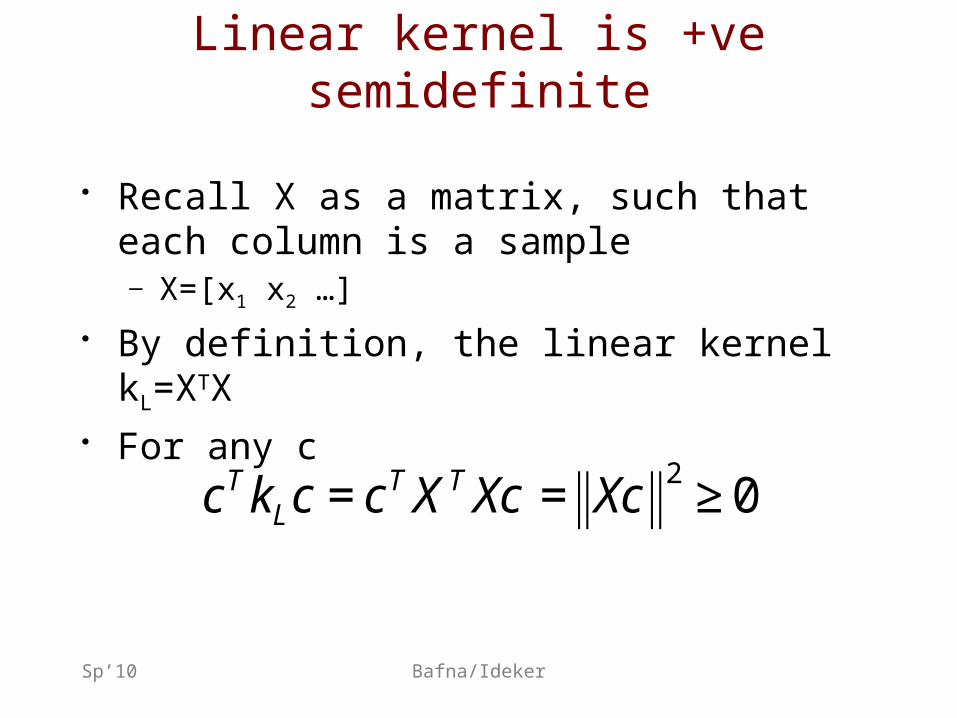
Linear kernel is +ve semidefinite

• Recall X as a matrix, such that each column is a sample– X=[x1 x2 …]

• By definition, the linear kernel kL=XTX• For any c

€

cT kLc = cTX TXc = Xc2

≥ 0


Generalizing kernels

• Any object can be represented by a feature vector in real space.

€

φ : X → R p

€

k(x,x ') = φ(x)T φ(x')


Generalizing

• Note that the feature mapping could actually be non-linear.

• On the flip side, Every kernel can be represented as a dot-product in a high dimensional space.

• Sometimes the kernel space is easier to define than the mapping


The kernel trick

• If an algorithm for vectorial data is expressed exclusively in the form of dot-products, it can be changed to an algorithm on an arbitrary kernel– Simply replace the dot-product by the kernel


Kernel trick example

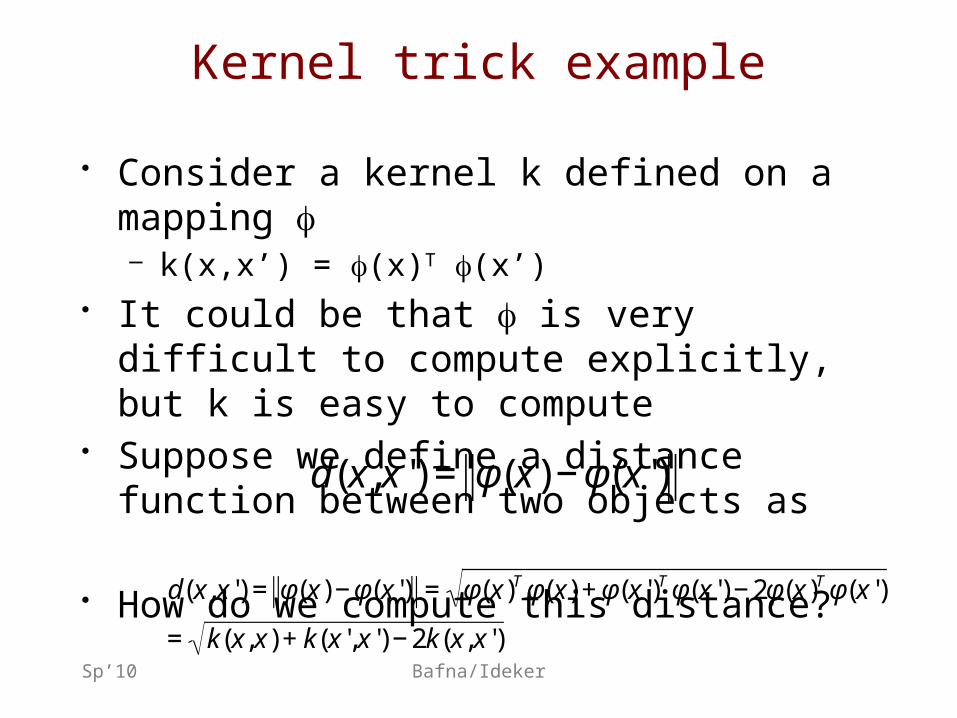
• Consider a kernel k defined on a mapping – k(x,x’) = (x)T (x’)

• It could be that is very difficult to compute explicitly, but k is easy to compute

• Suppose we define a distance function between two objects as

• How do we compute this distance?€

d(x,x ') = φ(x) −φ(x')

€

d(x,x ') = φ(x) −φ(x') = φ(x)T φ(x) + φ(x ')Tφ(x ') − 2φ(x)Tφ(x ')

= k(x,x) + k(x',x ') − 2k(x,x')


Kernels and SVMs

• Recall that SVM based classification is described as

€

min −1

2α iα jy iy jx i

T x ji, j

∑ + α ii∑

s.t.

y iα ii∑ = 0

0 ≤ α i ≤ C


Kernels and SVMs

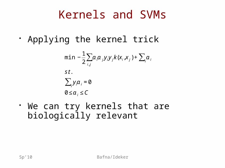
• Applying the kernel trick

• We can try kernels that are biologically relevant€

min −1

2α iα jy iy jk(x i

i, j

∑ ,x j ) + α ii∑

s.t.

y iα ii∑ = 0

0 ≤ α i ≤ C


Examples of kernels for vectors

€

linear kernel kL (x,x') = xT x '

€

poly kernel kp (x,x') = xT x'+c( )d

€

Gaussian RBF kernel kG (x,x') = exp −x − x '

2

2σ 2

⎛

⎝ ⎜ ⎜

⎞

⎠ ⎟ ⎟


String kernel

• Consider a string s = s1, s2,…

• Define an index set I as a subset of indices

• s[I] is the substring limited to those indices

• l(I) = span• W(I) = cl(I) c<1

– Weight decreases as span increases

• For any string u of length k

l(I)

€

φu(s) = c l(I )

I :s(I )= u

∑


String Kernel

• Map every string to a ||n dimensional space, indexed by all strings u of length upto n

• The mapping is expensive, but given two strings s,t,the dot-product kernel k(s,t) = (s)T(t) can be computed in O(n |s| |t|) time

€

φs u

€

φu(s)


SVM conclusion

• SVM are a generic scheme for classifying data with wide margins and low misclassifications

• For data that is not easily represented as vectors, the kernel trick provides a standard recipe for classification– Define a meaningful kernel, and solve using

SVM• Many standard kernels are available

(linear, poly., RBF, string)


Classification review

• We started out by treating the classification problem as one of separating points in high dimensional space

• Obvious for gene expression data, but applicable to any kind of data

• Question of separability, linear separation• Algorithms for classification

– Perceptron– Lin. Discriminant– Max Likelihood– Linear Programming– SVMs– Kernel methods & SVM


Classification review

• Recall that we considered 3 problems:– Group together samples in an unsupervised

fashion (clustering)– Classify based on a training data (often by

learning a hyperplane that separates).– Selection of marker genes that are

diagnostic for the class. All other genes can be discarded, leading to lower dimensionality.


Dimensionality reduction

• Many genes have highly correlated expression profiles.

• By discarding some of the genes, we can greatly reduce the dimensionality of the problem.

• There are other, more principled ways to do such dimensionality reduction.


Why is high dimensionality bad?

• With a high enough dimensionality, all points can be linearly separated.

• Recall that a point xi is misclassified if – it is +ve, but Txi-0<=0– it is -ve, but Txi+0 > 0

• In the first case choose i s.t. – Txi-0+i >= 0

• By adding a dimension for each misclassified point, we create a higher dimension hyperplane that perfectly separates all of the points!


Principle Components Analysis

• We get the intrinsic dimensionality of a data-set.


Principle Components Analysis

• Consider the expression values of 2 genes over 6 samples.

• Clearly, the expression of the two genes is highly correlated.

• Projecting all the genes on a single line could explain most of the data.

• This is a generalization of “discarding the gene”.


Projecting

• Consider the mean of all points m, and a vector emanating from the mean

• Algebraically, this projection on means that all samples x can be represented by a single value T(x-m)

m

x

x-m

T =

M

T(x-m)


Higher dimensions

• Consider a set of 2 (k) orthonormal vectors 1, 2…

• Once projected, each sample means that all samples x can be represented by 2 (k) dimensional vector– 1

T(x-m), 2T(x-m)

1m

x

x-m1

T

=

M

1T(x-m)

2


How to project

• The generic scheme allows us to project an m dimensional surface into a k dimensional one.

• How do we select the k ‘best’ dimensions?

• The strategy used by PCA is one that maximizes the variance of the projected points around the mean


PCA

• Suppose all of the data were to be reduced by projecting to a single line from the mean.

• How do we select the line ?

m


PCA cont’d

• Let each point xk map to x’k=m+ak. We want to minimize the error

• Observation 1: Each point xk maps to x’k = m + T(xk-m)– (ak= T(xk-m))€

xk − x 'k2

k

∑

m

xk

x’k


Proof of Observation 1

€

minak xk − x'k2

= minak xk −m + m − x'k2

= minak xk −m2

+ m − x'k2

− 2(x'k −m)T (xk −m)

= minak xk −m2

+ ak2β Tβ − 2akβ

T (xk −m)

= minak xk −m2

+ ak2 − 2akβ

T (xk −m)

€

2ak − 2β T (xk −m) = 0

ak = β T (xk −m)

⇒ ak2 = akβ

T (xk −m)

⇒ xk − x 'k2

= xk −m2

−β T (xk −m)(xk −m)T β

Differentiating w.r.t ak


Minimizing PCA Error

• To minimize error, we must maximize TS• By definition, = TS implies that is an eigenvalue, and

the corresponding eigenvector.• Therefore, we must choose the eigenvector

corresponding to the largest eigenvalue.

€

xk − x 'kk

∑2

=C − β T

k

∑ (xk −m)(xk −m)T β =C −β TSβ


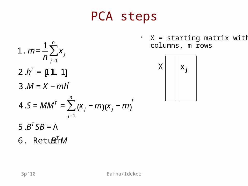
PCA steps• X = starting matrix with n

columns, m rows

xjX

€

1. m =1

nx j

j=1

n

∑

2. hT = 11L 1[ ]

3. M = X −mhT

4. S = MMT = x j −m( )j=1

n

∑ x j −m( )T

5. BTSB = Λ

6. Return BTM

End of Lecture



ALL-AML classification

• The two leukemias need different different therapeutic regimen.

• Usually distinguished through hematopathology

• Can Gene expression be used for a more definitive test?– 38 bonemarrow samples– Total mRNA was hybridized against probes for 6817

genes– Q: Are these classes separable


Neighborhood analysis (cont’d)

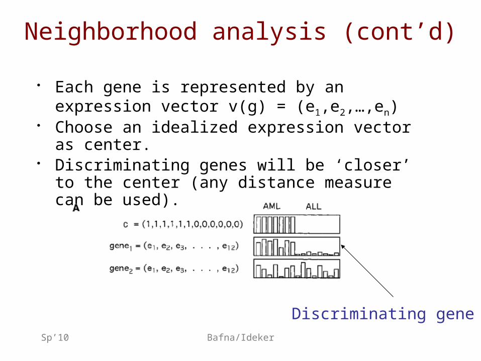
• Each gene is represented by an expression vector v(g) = (e1,e2,…,en)

• Choose an idealized expression vector as center.

• Discriminating genes will be ‘closer’ to the center (any distance measure can be used).

Discriminating gene


Neighborhood analysis

• Q: Are there genes, whose expression correlates with one of the two classes

• A: For each class, create an idealized vector c– Compute the number of genes Nc whose expression

‘matches’ the idealized expression vector– Is Nc significantly larger than Nc* for a random c*?


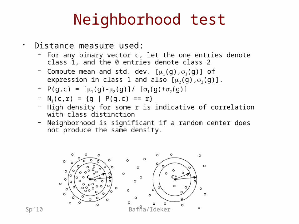
Neighborhood test• Distance measure used:

– For any binary vector c, let the one entries denote class 1, and the 0 entries denote class 2

– Compute mean and std. dev. [1(g),1(g)] of expression in class 1 and also [2(g),2(g)].

– P(g,c) = [1(g)-2(g)]/ [1(g)+2(g)] – N1(c,r) = {g | P(g,c) == r}– High density for some r is indicative of correlation with class

distinction– Neighborhood is significant if a random center does not

produce the same density.


Neighborhood analysis

• #{g |P(g,c) > 0.3} > 709 (ALL) vs 173 by chance.

• Class prediction should be possible using micro-array expression values.


Class prediction

• Choose a fixed set of informative genes (based on their correlation with the class distinction).– The predictor is uniquely defined by the sample and the subset

of informative genes.• For each informative gene g, define (wg,bg).

– wg=P(g,c) (When is this +ve?)– bg = [1(g)+2(g)]/2

• Given a new sample X– xg is the normalized expression value at g– Vote of gene g =wg|xg-bg| (+ve value is a vote for class 1, and

negative for class 2)


Prediction Strength

• PS = [Vwin-Vlose]/[Vwin+Vlose]– Reflects the margin of victory

• A 50 gene predictor is correct 36/38 (cross-validation)

• Prediction accuracy on other samples 100% (prediction made for 29/34 samples.

• Median PS = 0.73• Other predictors between 10 and 200 genes all

worked well.


Performance


Differentially expressed genes?

• Do the predictive genes reveal any biology?

• Initial expectation is that most genes would be of a hematopoetic lineage.

• However, many genes encode– Cell cycle progression genes– Chromatin remodelling– Transcription– Known oncogenes– Leukemia targets (etopside)


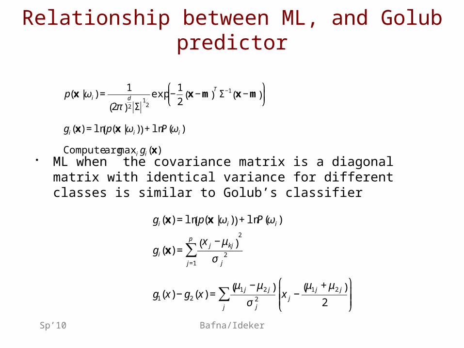
Relationship between ML, and Golub predictor

• ML when the covariance matrix is a diagonal matrix with identical variance for different classes is similar to Golub’s classifier€

p(x |ωi) =1

2π( )d

2 Σ1

2

exp −1

2x −m( )

TΣ−1 x −m( )

⎛

⎝ ⎜

⎞

⎠ ⎟

gi(x) = ln p(x |ωi)( ) + lnP(ωi)

Compute argmaxi gi(x)

€

gi(x) = ln p(x |ωi)( ) + lnP(ωi)

gi(x) =x j −μ kj( )

2

σ j2

j=1

p

∑

g1(x) − g2(x) =μ1 j −μ2 j( )

σ j2

x j −μ1 j + μ2 j( )

2

⎛

⎝ ⎜ ⎜

⎞

⎠ ⎟ ⎟

j

∑


Automatic class discovery

• The classification of different cancers is over years of hypothesis driven research.

• Suppose you were given unlabeled samples of ALL/AML. Would you be able to distinguish the two classes?


Self Organizing Maps

• SOMs was applied to group the 38 samples

• Class A1 contained 24/25 ALL and 3/13 AML samples.

• How can we validate this?• Use the labels to do supervised

classification via cross-validation• A 20 gene predictor gave 34 accurate

predictions, 1 error, and 2 of 3 uncertains


Comparing various error models


Conclusion

sp’10bafna/ideker classification (svms / kernel method)

Documents

object x x

x x r

objects x

sample x

point x

ve points x t x

sp10bafnaideker linear

sp10bafnaideker lp