the non-separable case non-linear svms and kernel methods...

CSCE 666 Pattern Analysis | Ricardo Gutierrez-Osuna | CSE@TAMU 1

L22: SVMs and kernel methods

• The non-separable case

• Non-linear SVMs and kernel methods

• A numerical example

• Optimization techniques

• SVM extensions

• Discussion


The non-separable case

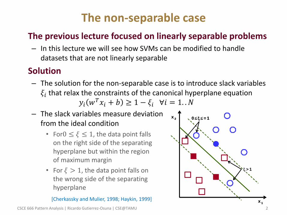
• The previous lecture focused on linearly separable problems – In this lecture we will see how SVMs can be modified to handle

datasets that are not linearly separable

• Solution – The solution for the non-separable case is to introduce slack variables 𝜉𝑖 that relax the constraints of the canonical hyperplane equation

𝑦𝑖 𝑤𝑇𝑥𝑖 + 𝑏 ≥ 1 − 𝜉𝑖 ∀𝑖 = 1. . 𝑁

– The slack variables measure deviation from the ideal condition

• For0 ≤ 𝜉 ≤ 1, the data point falls on the right side of the separating hyperplane but within the region of maximum margin

• For 𝜉 > 1, the data point falls on the wrong side of the separating hyperplane

[Cherkassky and Mulier, 1998; Haykin, 1999] x1

x2 0 = 1

> 1

x1

x2 0 = 1

> 1


The non-separable case

• How does the optimization problem change with the introduction of slack variables? – Our goal is to find a hyperplane with minimum misclassification rate

– This may be achieved by minimizing the following objective function

Θ 𝜉 = 𝐼 𝜉𝑖 − 1𝑁𝑖=1 𝑤ℎ𝑒𝑟𝑒 𝐼 𝜉𝑖 =

0; 𝜉 ≤ 01; 𝜉 > 0

• subject to the constraints on 𝑤 2 and the perceptron equation

– Θ 𝜉 represents the total number of misclassified samples

– Unfortunately, minimization of Θ 𝜉 is a difficult combinatorial problem (NP-complete) due to the non-linearity of the indicator function 𝐼 𝜉𝑖

[Cherkassky and Mulier, 1998]


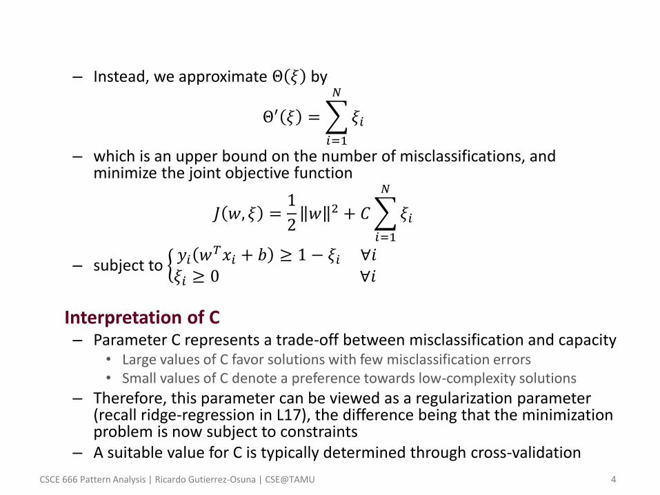
– Instead, we approximate Θ 𝜉 by

Θ′ 𝜉 = 𝜉𝑖

𝑁

𝑖=1

– which is an upper bound on the number of misclassifications, and minimize the joint objective function

𝐽 𝑤, 𝜉 =1

2𝑤 2 + 𝐶 𝜉𝑖

𝑁

𝑖=1

– subject to 𝑦𝑖 𝑤

𝑇𝑥𝑖 + 𝑏 ≥ 1 − 𝜉𝑖 ∀𝑖𝜉𝑖 ≥ 0 ∀𝑖

• Interpretation of C – Parameter C represents a trade-off between misclassification and capacity

• Large values of C favor solutions with few misclassification errors • Small values of C denote a preference towards low-complexity solutions

– Therefore, this parameter can be viewed as a regularization parameter (recall ridge-regression in L17), the difference being that the minimization problem is now subject to constraints

– A suitable value for C is typically determined through cross-validation


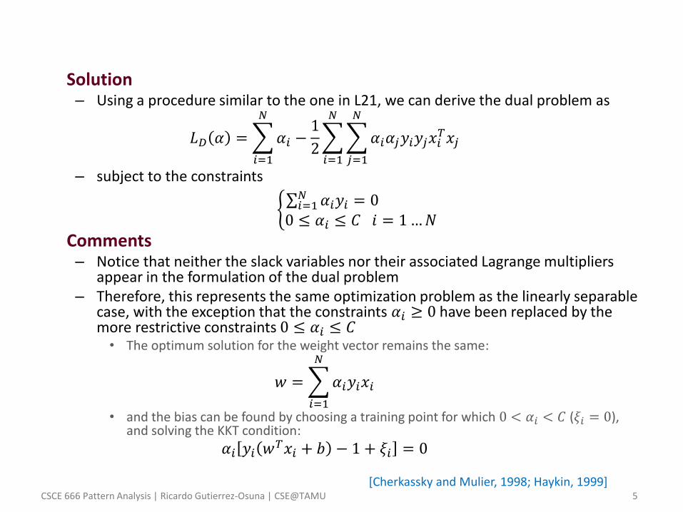
• Solution – Using a procedure similar to the one in L21, we can derive the dual problem as

𝐿𝐷 𝛼 = 𝛼𝑖 −1

2 𝛼𝑖𝛼𝑗𝑦𝑖𝑦𝑗𝑥𝑖

𝑇𝑥𝑗

𝑁

𝑗=1

𝑁

𝑖=1

𝑁

𝑖=1

– subject to the constraints

𝛼𝑖𝑦𝑖𝑁𝑖=1 = 0

0 ≤ 𝛼𝑖 ≤ 𝐶 𝑖 = 1…𝑁

• Comments – Notice that neither the slack variables nor their associated Lagrange multipliers

appear in the formulation of the dual problem – Therefore, this represents the same optimization problem as the linearly separable

case, with the exception that the constraints 𝛼𝑖 ≥ 0 have been replaced by the more restrictive constraints 0 ≤ 𝛼𝑖 ≤ 𝐶 • The optimum solution for the weight vector remains the same:

𝑤 = 𝛼𝑖𝑦𝑖𝑥𝑖

𝑁

𝑖=1

• and the bias can be found by choosing a training point for which 0 < 𝛼𝑖 < 𝐶 (𝜉𝑖 = 0), and solving the KKT condition:

𝛼𝑖 𝑦𝑖 𝑤𝑇𝑥𝑖 + 𝑏 − 1 + 𝜉𝑖 = 0

[Cherkassky and Mulier, 1998; Haykin, 1999]


Non-linear SVMs

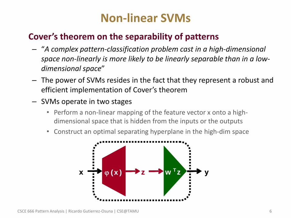
• Cover’s theorem on the separability of patterns – “A complex pattern-classification problem cast in a high-dimensional

space non-linearly is more likely to be linearly separable than in a low-dimensional space”

– The power of SVMs resides in the fact that they represent a robust and efficient implementation of Cover’s theorem

– SVMs operate in two stages

• Perform a non-linear mapping of the feature vector x onto a high-dimensional space that is hidden from the inputs or the outputs

• Construct an optimal separating hyperplane in the high-dim space

x (x ) z w T z yx (x ) z w T z y


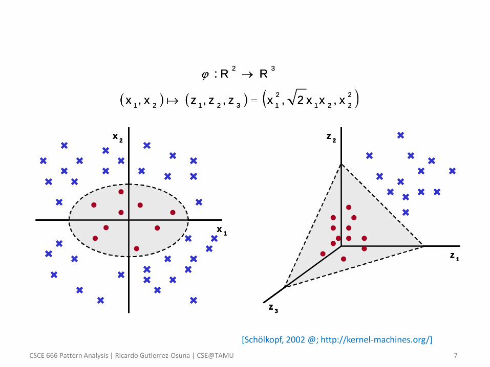
2

221

2

132121

32

x,xx2,xz,z,zx,x

RR:

x1

x2

z1

z2

z3

2

221

2

132121

32

x,xx2,xz,z,zx,x

RR:

x1

x2

x1

x2

z1

z2

z3

z1

z2

z3

[Schölkopf, 2002 @; http://kernel-machines.org/]


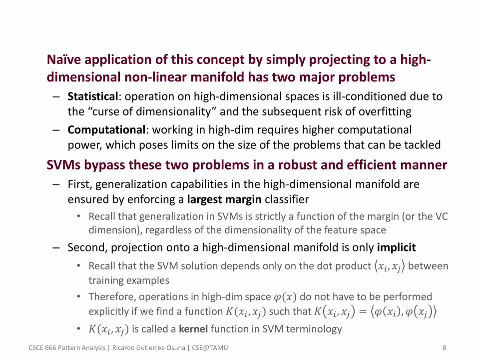
• Naïve application of this concept by simply projecting to a high-dimensional non-linear manifold has two major problems

– Statistical: operation on high-dimensional spaces is ill-conditioned due to the “curse of dimensionality” and the subsequent risk of overfitting

– Computational: working in high-dim requires higher computational power, which poses limits on the size of the problems that can be tackled

• SVMs bypass these two problems in a robust and efficient manner

– First, generalization capabilities in the high-dimensional manifold are ensured by enforcing a largest margin classifier

• Recall that generalization in SVMs is strictly a function of the margin (or the VC dimension), regardless of the dimensionality of the feature space

– Second, projection onto a high-dimensional manifold is only implicit

• Recall that the SVM solution depends only on the dot product 𝑥𝑖 , 𝑥𝑗 between

training examples

• Therefore, operations in high-dim space 𝜑(𝑥) do not have to be performed

explicitly if we find a function 𝐾(𝑥𝑖 , 𝑥𝑗) such that 𝐾 𝑥𝑖 , 𝑥𝑗 = 𝜑 𝑥𝑖 , 𝜑 𝑥𝑗

• 𝐾(𝑥𝑖 , 𝑥𝑗) is called a kernel function in SVM terminology


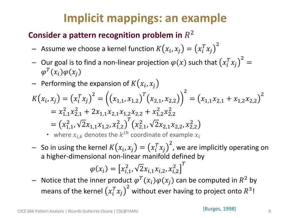
Implicit mappings: an example • Consider a pattern recognition problem in 𝑅2

– Assume we choose a kernel function 𝐾 𝑥𝑖 , 𝑥𝑗 = 𝑥𝑖𝑇𝑥𝑗

2

– Our goal is to find a non-linear projection 𝜑(𝑥) such that 𝑥𝑖𝑇𝑥𝑗

2=

𝜑𝑇(𝑥𝑖)𝜑(𝑥𝑗)

– Performing the expansion of 𝐾 𝑥𝑖 , 𝑥𝑗

𝐾 𝑥𝑖 , 𝑥𝑗 = 𝑥𝑖𝑇𝑥𝑗

2= 𝑥1,1, 𝑥1,2

𝑇𝑥2,1, 𝑥2,2

2

= 𝑥1,1𝑥2,1 + 𝑥1,2𝑥2,22

= 𝑥1,12 𝑥2,1

2 + 2𝑥1,1𝑥2,1𝑥1,2𝑥2,2 + 𝑥1,22 𝑥2,2

2

= 𝑥1,12 , 2𝑥1,1𝑥1,2, 𝑥1,2

2𝑇𝑥2,12 , 2𝑥2,1𝑥2,2, 𝑥2,2

2

• where 𝑥𝑖,𝑘 denotes the 𝑘𝑡ℎ coordinate of example 𝑥𝑖

– So in using the kernel 𝐾 𝑥𝑖 , 𝑥𝑗 = 𝑥𝑖𝑇𝑥𝑗

2, we are implicitly operating on

a higher-dimensional non-linear manifold defined by

𝜑 𝑥𝑖 = 𝑥𝑖,12 , 2𝑥𝑖,1𝑥𝑖,2, 𝑥𝑖,2

2 𝑇

– Notice that the inner product 𝜑𝑇(𝑥𝑖)𝜑(𝑥𝑗) can be computed in 𝑅2 by

means of the kernel 𝑥𝑖𝑇𝑥𝑗

2 without ever having to project onto 𝑅3!

[Burges, 1998]


Kernel methods

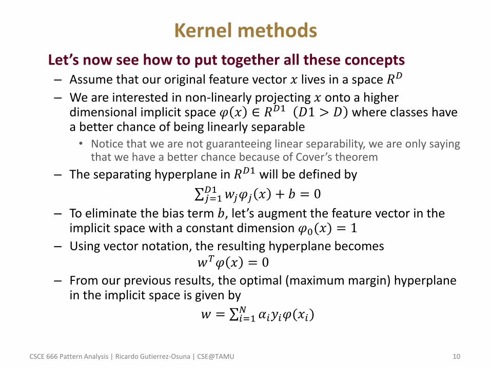
• Let’s now see how to put together all these concepts – Assume that our original feature vector 𝑥 lives in a space 𝑅𝐷

– We are interested in non-linearly projecting 𝑥 onto a higher dimensional implicit space 𝜑 𝑥 ∈ 𝑅𝐷1 𝐷1 > 𝐷 where classes have a better chance of being linearly separable • Notice that we are not guaranteeing linear separability, we are only saying

that we have a better chance because of Cover’s theorem

– The separating hyperplane in 𝑅𝐷1 will be defined by

𝑤𝑗𝜑𝑗 𝑥 + 𝑏𝐷1𝑗=1 = 0

– To eliminate the bias term 𝑏, let’s augment the feature vector in the implicit space with a constant dimension 𝜑0(𝑥) = 1

– Using vector notation, the resulting hyperplane becomes 𝑤𝑇𝜑 𝑥 = 0

– From our previous results, the optimal (maximum margin) hyperplane in the implicit space is given by

𝑤 = 𝛼𝑖𝑦𝑖𝜑(𝑥𝑖)𝑁𝑖=1


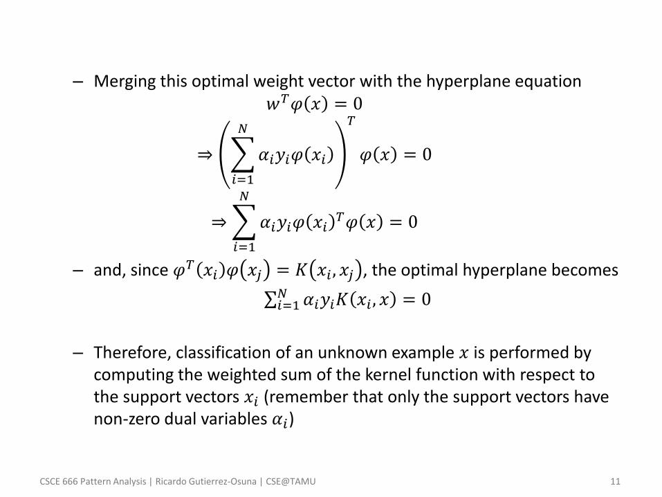
– Merging this optimal weight vector with the hyperplane equation 𝑤𝑇𝜑 𝑥 = 0

⇒ 𝛼𝑖𝑦𝑖𝜑 𝑥𝑖

𝑁

𝑖=1

𝑇

𝜑 𝑥 = 0

⇒ 𝛼𝑖𝑦𝑖𝜑 𝑥𝑖𝑇𝜑 𝑥

𝑁

𝑖=1

= 0

– and, since 𝜑𝑇 𝑥𝑖 𝜑 𝑥𝑗 = 𝐾 𝑥𝑖 , 𝑥𝑗 , the optimal hyperplane becomes

𝛼𝑖𝑦𝑖𝐾 𝑥𝑖 , 𝑥 = 0𝑁𝑖=1

– Therefore, classification of an unknown example 𝑥 is performed by computing the weighted sum of the kernel function with respect to the support vectors 𝑥𝑖 (remember that only the support vectors have non-zero dual variables 𝛼𝑖)


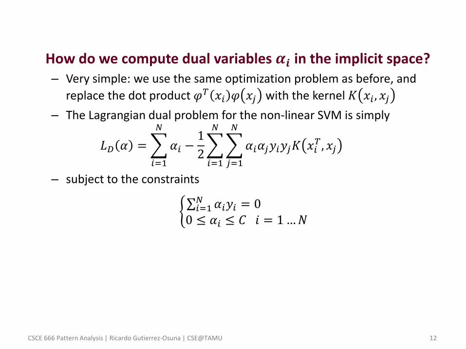
• How do we compute dual variables 𝜶𝒊 in the implicit space? – Very simple: we use the same optimization problem as before, and

replace the dot product 𝜑𝑇 𝑥𝑖 𝜑 𝑥𝑗 with the kernel 𝐾 𝑥𝑖 , 𝑥𝑗

– The Lagrangian dual problem for the non-linear SVM is simply

𝐿𝐷 𝛼 = 𝛼𝑖 −1

2 𝛼𝑖𝛼𝑗𝑦𝑖𝑦𝑗𝐾 𝑥𝑖

𝑇 , 𝑥𝑗

𝑁

𝑗=1

𝑁

𝑖=1

𝑁

𝑖=1

– subject to the constraints

𝛼𝑖𝑦𝑖𝑁𝑖=1 = 0

0 ≤ 𝛼𝑖 ≤ 𝐶 𝑖 = 1…𝑁


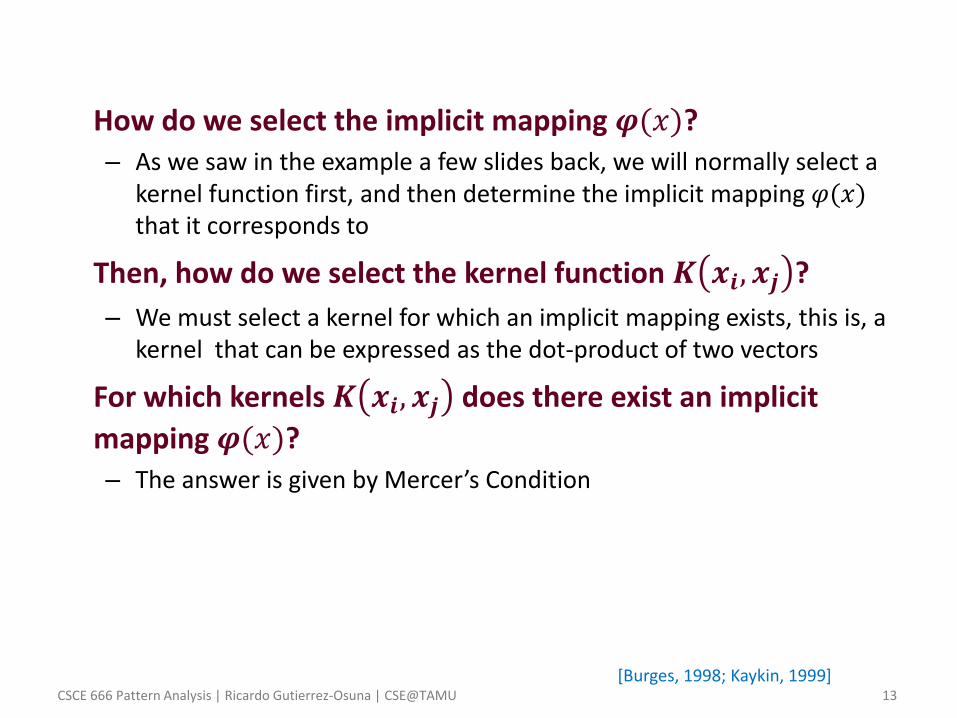
• How do we select the implicit mapping 𝝋(𝑥)? – As we saw in the example a few slides back, we will normally select a

kernel function first, and then determine the implicit mapping 𝜑(𝑥) that it corresponds to

• Then, how do we select the kernel function 𝑲 𝒙𝒊, 𝒙𝒋 ?

– We must select a kernel for which an implicit mapping exists, this is, a kernel that can be expressed as the dot-product of two vectors

• For which kernels 𝑲 𝒙𝒊, 𝒙𝒋 does there exist an implicit

mapping 𝝋(𝑥)? – The answer is given by Mercer’s Condition

[Burges, 1998; Kaykin, 1999]


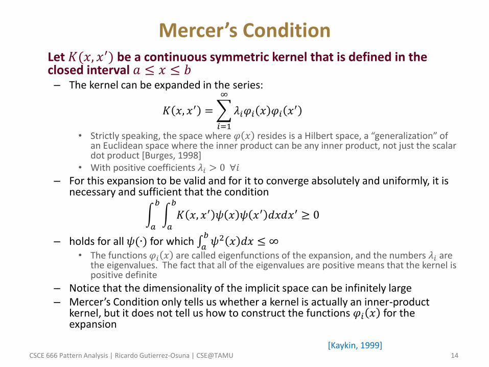
Mercer’s Condition • Let 𝐾(𝑥, 𝑥′) be a continuous symmetric kernel that is defined in the

closed interval 𝑎 ≤ 𝑥 ≤ 𝑏 – The kernel can be expanded in the series:

𝐾 𝑥, 𝑥′ = 𝜆𝑖𝜑𝑖 𝑥 𝜑𝑖 𝑥′

∞

𝑖=1

• Strictly speaking, the space where 𝜑 𝑥 resides is a Hilbert space, a “generalization” of an Euclidean space where the inner product can be any inner product, not just the scalar dot product [Burges, 1998]

• With positive coefficients 𝜆𝑖 > 0 ∀𝑖

– For this expansion to be valid and for it to converge absolutely and uniformly, it is necessary and sufficient that the condition

𝐾 𝑥, 𝑥′ 𝜓 𝑥 𝜓 𝑥′ 𝑑𝑥𝑑𝑥′𝑏

𝑎

≥ 0𝑏

𝑎

– holds for all 𝜓(∙) for which 𝜓2 𝑥 𝑑𝑥𝑏

𝑎≤ ∞

• The functions 𝜑𝑖 𝑥 are called eigenfunctions of the expansion, and the numbers 𝜆𝑖 are the eigenvalues. The fact that all of the eigenvalues are positive means that the kernel is positive definite

– Notice that the dimensionality of the implicit space can be infinitely large – Mercer’s Condition only tells us whether a kernel is actually an inner-product

kernel, but it does not tell us how to construct the functions 𝜑𝑖 𝑥 for the expansion

[Kaykin, 1999]


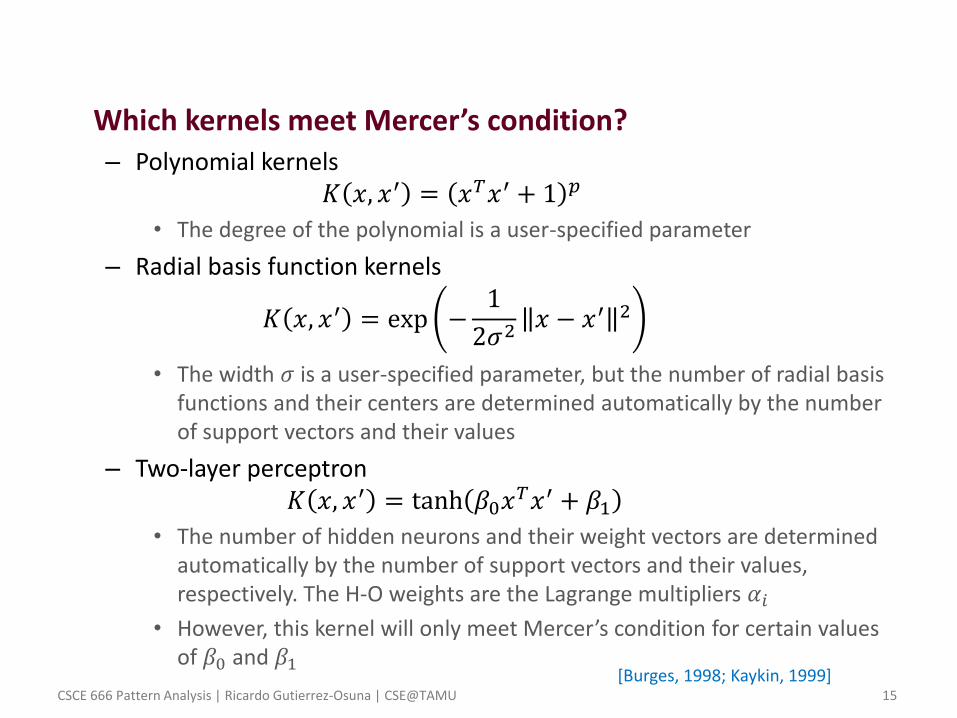
• Which kernels meet Mercer’s condition? – Polynomial kernels

𝐾 𝑥, 𝑥′ = 𝑥𝑇𝑥′ + 1 𝑝

• The degree of the polynomial is a user-specified parameter

– Radial basis function kernels

𝐾 𝑥, 𝑥′ = exp −1

2𝜎2𝑥 − 𝑥′ 2

• The width 𝜎 is a user-specified parameter, but the number of radial basis functions and their centers are determined automatically by the number of support vectors and their values

– Two-layer perceptron 𝐾 𝑥, 𝑥′ = tanh 𝛽0𝑥

𝑇𝑥′ + 𝛽1

• The number of hidden neurons and their weight vectors are determined automatically by the number of support vectors and their values, respectively. The H-O weights are the Lagrange multipliers 𝛼𝑖

• However, this kernel will only meet Mercer’s condition for certain values of 𝛽0 and 𝛽1

[Burges, 1998; Kaykin, 1999]


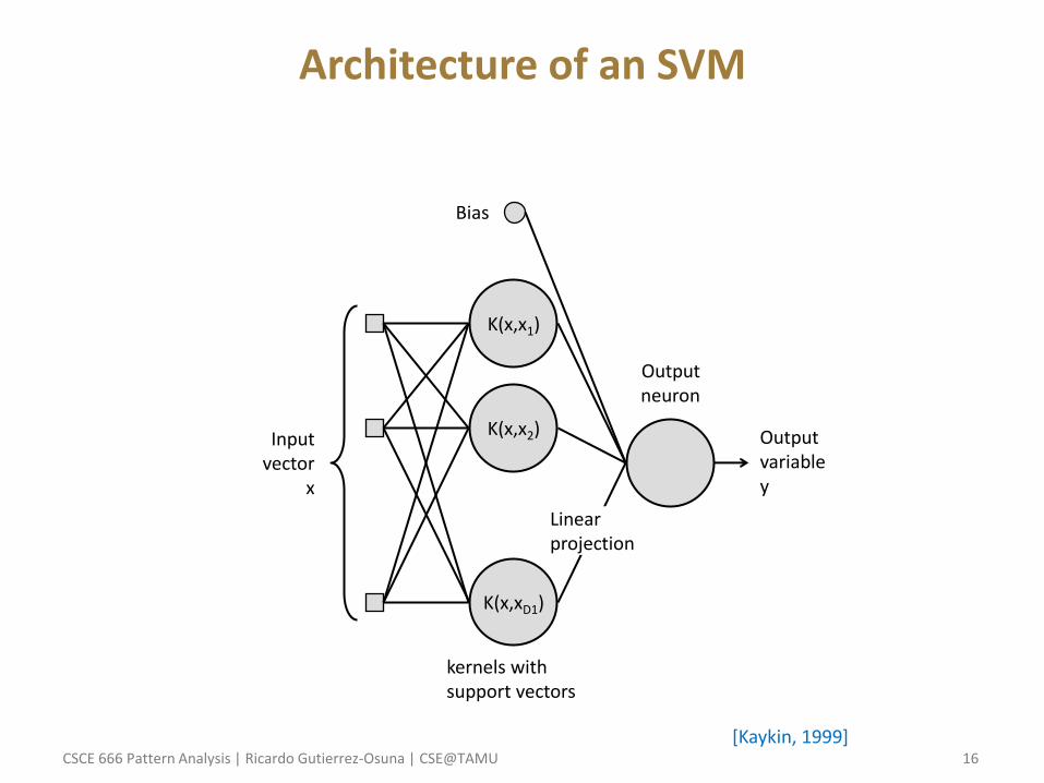
Architecture of an SVM

K(x,x1)

K(x,x2)

K(x,xD1)

Input vector

x

Bias

Output neuron

Linear projection

Output variable y

kernels with support vectors

[Kaykin, 1999]


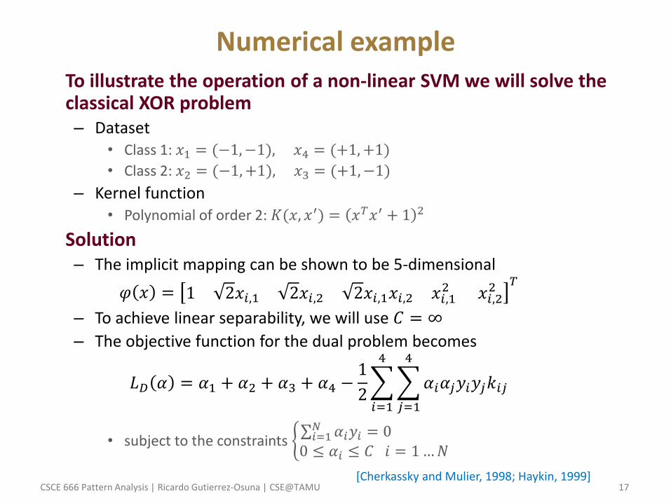
Numerical example • To illustrate the operation of a non-linear SVM we will solve the

classical XOR problem – Dataset

• Class 1: 𝑥1 = (−1,−1), 𝑥4 = (+1,+1)

• Class 2: 𝑥2 = (−1,+1), 𝑥3 = (+1,−1)

– Kernel function • Polynomial of order 2: 𝐾(𝑥, 𝑥′) = 𝑥𝑇𝑥′ + 1 2

• Solution – The implicit mapping can be shown to be 5-dimensional

𝜑 𝑥 = 1 2𝑥𝑖,1 2𝑥𝑖,2 2𝑥𝑖,1𝑥𝑖,2 𝑥𝑖,12 𝑥𝑖,2

2 𝑇

– To achieve linear separability, we will use 𝐶 = ∞

– The objective function for the dual problem becomes

𝐿𝐷 𝛼 = 𝛼1 + 𝛼2 + 𝛼3 + 𝛼4 −1

2 𝛼𝑖𝛼𝑗𝑦𝑖𝑦𝑗𝑘𝑖𝑗

4

𝑗=1

4

𝑖=1

• subject to the constraints 𝛼𝑖𝑦𝑖𝑁𝑖=1 = 0

0 ≤ 𝛼𝑖 ≤ 𝐶 𝑖 = 1…𝑁

[Cherkassky and Mulier, 1998; Haykin, 1999]


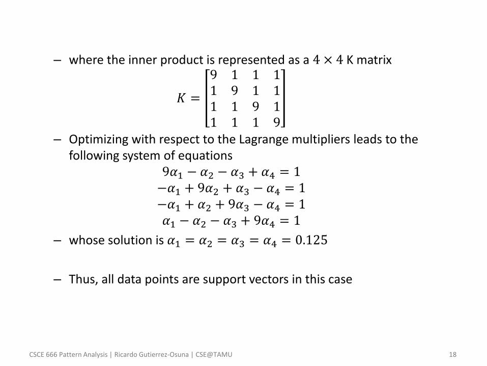
– where the inner product is represented as a 4 × 4 K matrix

𝐾 =

9 1 1 11 9 1 11 1 9 11 1 1 9

– Optimizing with respect to the Lagrange multipliers leads to the following system of equations

9𝛼1 − 𝛼2 − 𝛼3 + 𝛼4 = 1 −𝛼1 + 9𝛼2 + 𝛼3 − 𝛼4 = 1 −𝛼1 + 𝛼2 + 9𝛼3 − 𝛼4 = 1 𝛼1 − 𝛼2 − 𝛼3 + 9𝛼4 = 1

– whose solution is 𝛼1 = 𝛼2 = 𝛼3 = 𝛼4 = 0.125

– Thus, all data points are support vectors in this case


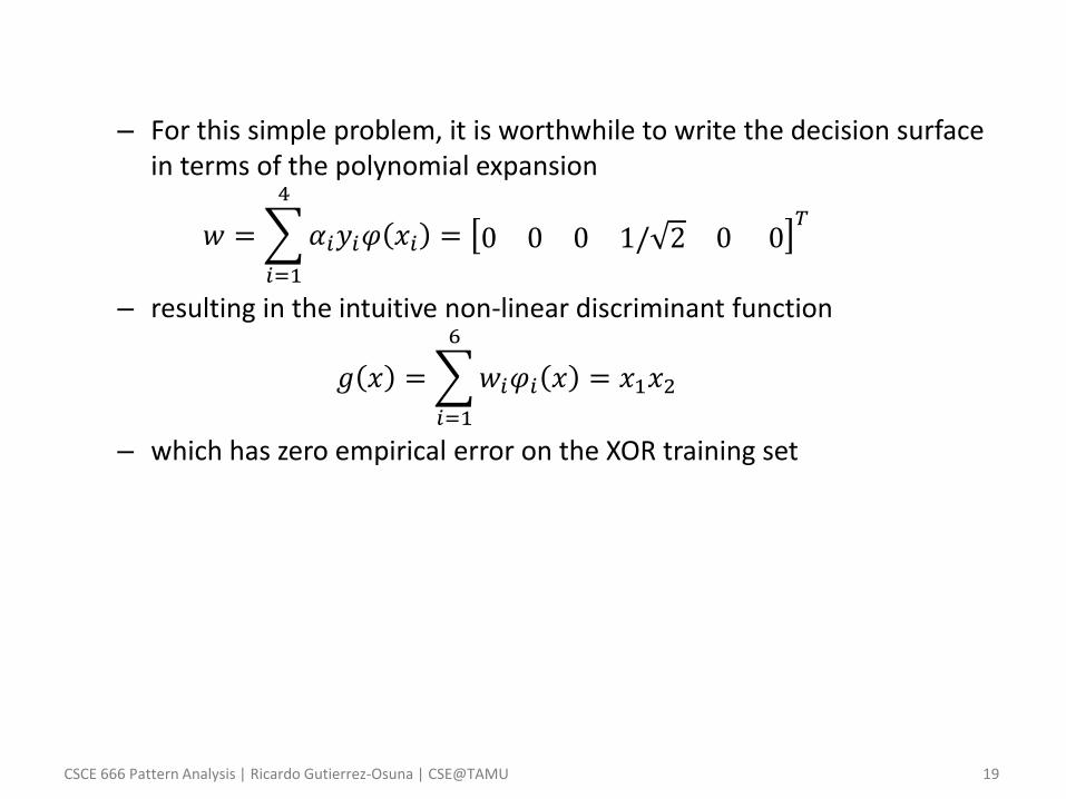
– For this simple problem, it is worthwhile to write the decision surface in terms of the polynomial expansion

𝑤 = 𝛼𝑖𝑦𝑖𝜑 𝑥𝑖

4

𝑖=1

= 0 0 0 1/ 2 0 0𝑇

– resulting in the intuitive non-linear discriminant function

𝑔 𝑥 = 𝑤𝑖𝜑𝑖 𝑥

6

𝑖=1

= 𝑥1𝑥2

– which has zero empirical error on the XOR training set


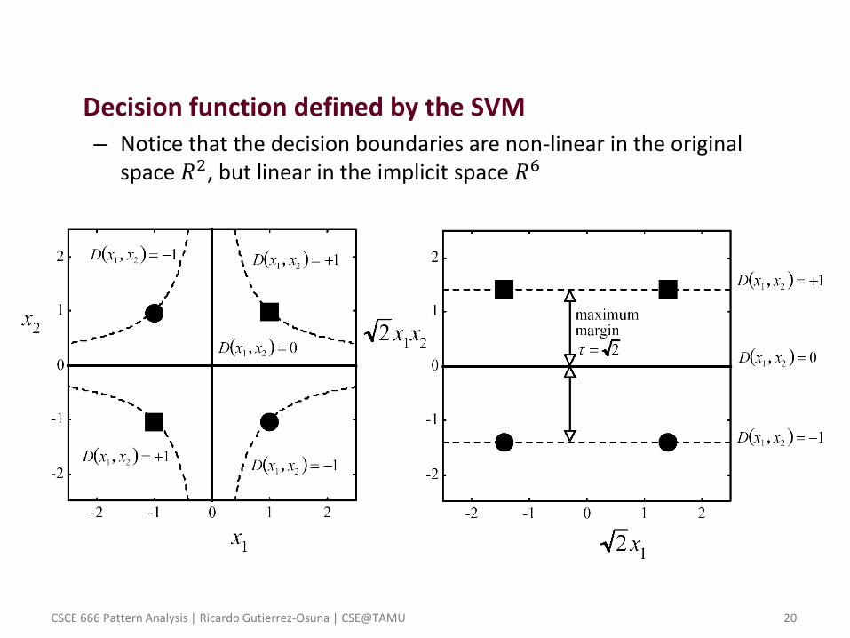
• Decision function defined by the SVM – Notice that the decision boundaries are non-linear in the original

space 𝑅2, but linear in the implicit space 𝑅6


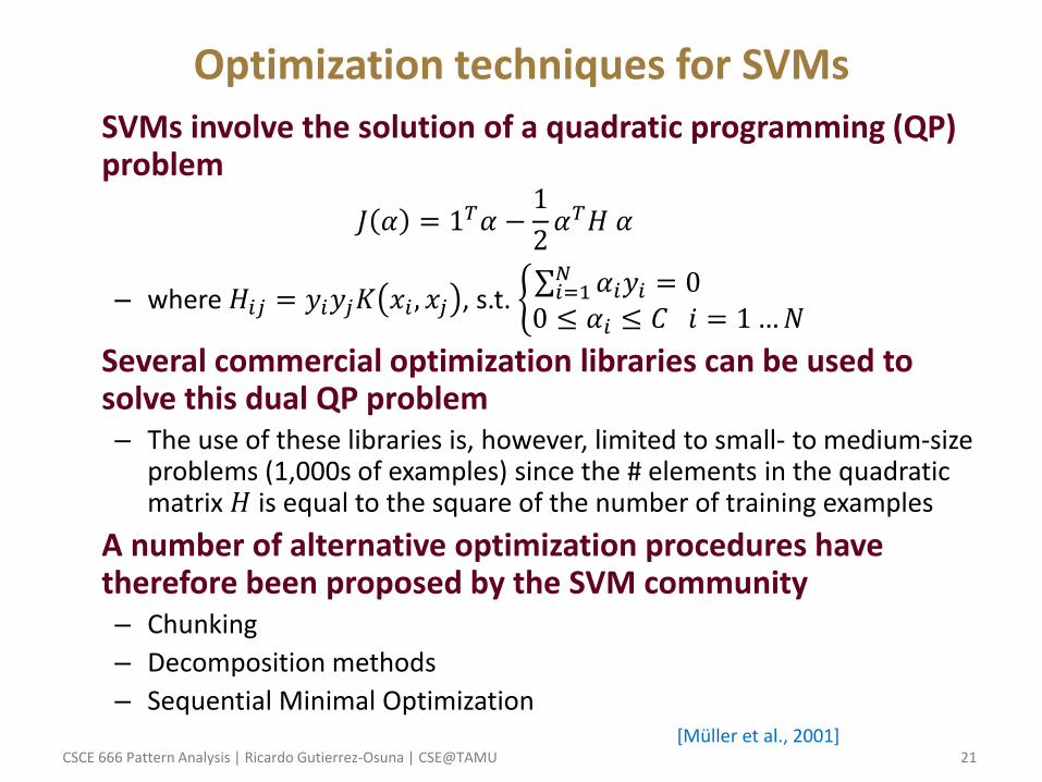
Optimization techniques for SVMs

• SVMs involve the solution of a quadratic programming (QP) problem

𝐽 𝛼 = 1𝑇𝛼 −1

2𝛼𝑇𝐻 𝛼

– where 𝐻𝑖𝑗 = 𝑦𝑖𝑦𝑗𝐾 𝑥𝑖 , 𝑥𝑗 , s.t. 𝛼𝑖𝑦𝑖𝑁𝑖=1 = 0

0 ≤ 𝛼𝑖 ≤ 𝐶 𝑖 = 1…𝑁

• Several commercial optimization libraries can be used to solve this dual QP problem – The use of these libraries is, however, limited to small- to medium-size

problems (1,000s of examples) since the # elements in the quadratic matrix 𝐻 is equal to the square of the number of training examples

• A number of alternative optimization procedures have therefore been proposed by the SVM community – Chunking

– Decomposition methods

– Sequential Minimal Optimization

[Müller et al., 2001]


• Chunking – This method is based on two facts

• Many of the optimal 𝛼s will be zero (or on the upper bound C). The QP solution is independent of these zero parameters, so their corresponding rows and columns in the quadratic matrix can be eliminated

• In addition, the optimal 𝛼s must meet the KKT condition

– At every step, chunking will solve a problem containing all the non-zero 𝛼s plus some of the 𝛼s that violate the KKT condition

– The size of the problem varies with every iteration, but is finally equal to the number of support vectors

– However, chunking is still limited by the maximum number of support vectors that fit in memory

– In addition, chunking requires an inner QP optimizer to solve each of the smaller problems


• Decomposition methods – Decomposition methods are similar to chunking in concept, except for

the size of the sub-problems is always fixed

– These methods are based on the fact that a sequence of QPs which contain at least one sample violating the KKT conditions will eventually converge to an optimal solution

– The original algorithm suggests adding and removing one example at every step, but this leads to very slow convergence

– Practical implementations use various heuristics to add or remove multiple examples at a time

– Decomposition methods still require an inner QP solver for the sub-problems


• Sequential Minimal Optimization (SMO) – This algorithm represents the extreme case of a decomposition

method: at every iteration SMO solves a QP problem of size TWO. This has two advantages

• A QP problem of size two can be solved analytically; no QP solver is required

• No extra matrix storage is required

– The main problem in SMO is how to choose a good pair of variables to optimize at every iteration. This is accomplished with a number of heuristics

– The implementation of SMO is straightforward, and the pseudo-code is even available [Platt, 1999]


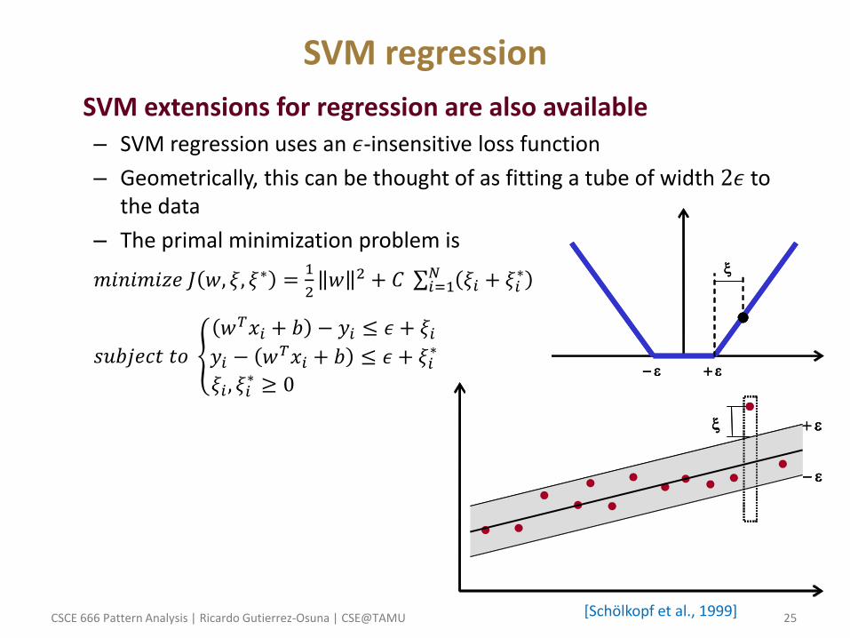
SVM regression

• SVM extensions for regression are also available – SVM regression uses an 𝜖-insensitive loss function

– Geometrically, this can be thought of as fitting a tube of width 2𝜖 to the data

– The primal minimization problem is

𝑚𝑖𝑛𝑖𝑚𝑖𝑧𝑒 𝐽 𝑤, 𝜉, 𝜉∗ =1

2𝑤 2 + 𝐶 𝜉𝑖 + 𝜉𝑖

∗𝑁𝑖=1

𝑠𝑢𝑏𝑗𝑒𝑐𝑡 𝑡𝑜

𝑤𝑇𝑥𝑖 + 𝑏 − 𝑦𝑖 ≤ 𝜖 + 𝜉𝑖𝑦𝑖 − 𝑤𝑇𝑥𝑖 + 𝑏 ≤ 𝜖 + 𝜉𝑖

∗

𝜉𝑖 , 𝜉𝑖∗ ≥ 0

[Schölkopf et al., 1999]


Kernel PCA

• SMVs can also be used to perform non-linear PCA – In this case, the problem involves the computation of eigenvectors and

eigenvalues of the SVM Kernel matrix 𝐾 𝑥𝑖 , 𝑥𝑗 = 𝜑 𝑥𝑖 , 𝜑 𝑥𝑗

– Because Kernel PCA is implicitly performed in a high-dimensional feature space, it can extract more features that those available in the original feature space (see example below)

– Similarly, SMV extensions to Fisher’s LDA are also available

First 8 non-linear principal components from a 2-dimensional dataset (from [Schölkopf et al., 1996])


Discussion

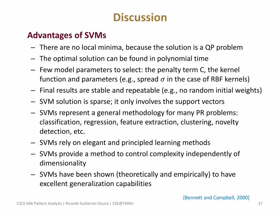
• Advantages of SVMs – There are no local minima, because the solution is a QP problem

– The optimal solution can be found in polynomial time

– Few model parameters to select: the penalty term C, the kernel function and parameters (e.g., spread 𝜎 in the case of RBF kernels)

– Final results are stable and repeatable (e.g., no random initial weights)

– SVM solution is sparse; it only involves the support vectors

– SVMs represent a general methodology for many PR problems: classification, regression, feature extraction, clustering, novelty detection, etc.

– SVMs rely on elegant and principled learning methods

– SVMs provide a method to control complexity independently of dimensionality

– SVMs have been shown (theoretically and empirically) to have excellent generalization capabilities

[Bennett and Campbell, 2000]


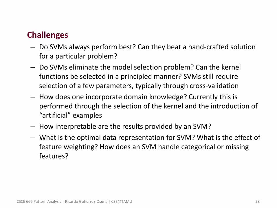
• Challenges – Do SVMs always perform best? Can they beat a hand-crafted solution

for a particular problem?

– Do SVMs eliminate the model selection problem? Can the kernel functions be selected in a principled manner? SVMs still require selection of a few parameters, typically through cross-validation

– How does one incorporate domain knowledge? Currently this is performed through the selection of the kernel and the introduction of “artificial” examples

– How interpretable are the results provided by an SVM?

– What is the optimal data representation for SVM? What is the effect of feature weighting? How does an SVM handle categorical or missing features?

the non-separable case non-linear svms and kernel methods...

Documents