lecture 4: quantitative spatial economicserossi/trade/lecture4_552.pdfi in the spirit of the seminal...

Lecture 4: Quantitative Spatial EconomicsEconomics 552

Esteban Rossi-Hansberg

Princeton University

ERH (Princeton University ) Lecture 4: Quantitative Spatial Economics 1 / 41

Redding and Rossi-Hansberg

Economic activity is highly unevenly distributed across space, as reflected inthe existence of cities

The delicate balance between agglomeration and dispersion forces thatunderlie these concentrations of economic activity is central to a range ofeconomic phenomena

I incomes of mobile and immobile factorsI the magnitude of residential amenitiesI investments,I and city and aggregate productivity

The impact of public policy interventions is crucially determined by how thesepolicies affect the equilibrium balance between these centripetal andcentrifugal forces in a realistic context

I transport infrastructure investmentsI local taxationI land regulationI place-based policies


Introduction

Theoretical literature on economic geography has traditionally focused onstylized settings that cannot easily be taken to the data

More recent research has developed quantitative models of the spatialdistribution of economic activity

I Rich enough to incorporate first-order features of the dataF Large numbers of locations with heterogenous geography, productivity,amenities, local factors

F Trade in goods, migration, and commuting

I Suffi ciently tractable as to enable quantitative counterfactuals to evaluatenumerically, in a realistic setup, a variety of policies and counterfactualscenarios


Introduction

Early theoretical research on new economic geography concentrated onformalizing mechanisms for agglomeration and cumulative causation

I Fujita, et al. 1999, Fujita and Thisse 2002 and Baldwin et al. 2003

This literature stressed the combination of love of variety, increasing returnsto scale and transport costs as a mechanism for agglomeration forces

I Provided a fundamental theoretical explanation for the emergence of anuneven distribution of economic activity even on a featureless plain of ex anteidentical locations

F multiple equilibria in location choicesF Alternative was to incorporate externalities

Theoretical literature stimulated a wave of empirical research, much of thisempirical research was reduced-form in nature

I Mapping from the model to the empirical specification was often unclearI Coeffi cients of these reduced-form relationships need not be invariant to policyintervention (the Lucas Critique)

I Inability to evaluate welfare effects of policy


Introduction

More recent research in economic geography has developed a quantitativeframework that connects closely to the observed data

I Following the introduction of quantitative models of international trade (inparticular Eaton and Kortum, 2002)

Does not aim to provide a fundamental explanation for the agglomeration ofeconomic activity

I Agglomeration in these models is simply the result of exogenous localcharacteristics, augmented by endogenous economic mechanisms

These frameworks can accommodate many realistic features and can bemade quite rich

The same quantitative framework can be derived from an entire class oftheoretical models of economic geography


Introduction

The close connection between model and data in this quantitative researchhas a number of advantages:

I Through accommodating many regions and a rich geography of trade costs,these models provide microfoundations for central features of the data

I Explain the observed data as an equilibrium of the modelI Models are typically exactly identified: one-to-one mapping from the observeddata and exogenous primitives or structural fundamentals of the model

F Can be inverted to identify the unique values of the structural fundamentalsF Observed variation in the data can be decomposed within the model into thecontributions of each fundamental


Introduction

A central advantage is the ability to undertake counterfactuals for policyinterventions or other out of sample changes in model primitives

I Assuming identified structural fundamentals are stable and invariant to theanalyzed policy interventions

Yield general equilibrium predictions for the spatial distribution of economicactivity

I Take full account of all the complex spatial interactions between locations

Key implication of this analysis is that locations are not independentobservations in a cross-section regression, but are rather systematically linkedto one another through trade, commuting and migrations flows

Use of the model’s structure makes it possible to compute the counterfactualchange in welfare


A Menu of Quantitative Spatial Models

All quantitative spatial models implicitly or explicitly makes assumptionsabout a number of building blocks:

1 Preferences2 Production Technology3 Technology for Trading Goods4 Technology for Idea Flows5 Technology for the movement of people6 Endowments7 Equilibrium


A Menu of QSM: Preferences

1 Homogeneous versus differentiated goods (love of variety)2 Single versus multiple sectors3 Exogenous amenities (e.g scenic views) and/or endogenous amenities (e.g.crime)

I In the spirit of the seminal work of Rosen (1979) and Roback (1982),amenities are understood as any characteristic that makes a location a moredesirable place of residence

4 Fixed local factors in utility (residential land use)5 Common versus idiosyncratic preferences

I Idiosyncratic preferences for each location that are typically modelled as beingdrawn from an extreme value distribution


A Menu of QSM: Production Technology

1 Constant versus increasing returns2 Exogenous productivity differences (e.g. mineral resources) and/orendogenous productivity differences (e.g. knowledge spillovers)

I Quantitative spatial models have typically found it necessary to allow for suchexogenous differences across locations in order to rationalize the observedemployment and income data

3 Input-output linkages4 Fixed local factors in production (commercial land use)


A Menu of QSM: Technology for Trading Goods

1 Variable versus fixed trade costsI A widespread assumption for analytical tractability is iceberg variable transportcosts, whereby dni ≥ 1 units of a good must be shipped from location i tolocation n in order for one unit to arrive

I Important to be consistent with the gravity equation (bilateral trade increaseswith exporter and importer size and declines with distance)

2 Asymmetric versus symmetric transport costs3 Geographic (e.g. mountains) versus economic frictions (e.g. borders, roadand rail networks)

4 Non-traded goods


A Menu of QSM: Technology for Idea Flows

1 Knowledge externalities and diffusionI Whenever an economic agent takes an action that affects another economicagent and this effect is not internalized when evaluating the cost and benefitsof the action

I The standard classification of these microfoundations is due to Marshall(1920) and distinguishes between knowledge spillovers, externalities due tothick labor markets, and backward and forward linkages

2 InnovationI Level of local productivity can be constant and exogenous, or the result ofintentional investments in innovation

I The incentives to undertake these investments depend on the market size andtherefore on the distribution of economic activity

3 Transferability of ideasI Extent to which ideas developed in one location can be costlessly transferredto other locations


A Menu of QSM: Technology for the movement of people

1 Migration costs2 Commuting and commuting costs

I Whether agents can separate their workplace and residence by commutingbetween them

I Standard in urban but not in regional models

3 Agent heterogeneityI Determines the need to track people as they switch locations

4 Congestion in transportation


A Menu of QSM: Endowments

1 Population and skills2 Spatial scope and units

I In most cases, geographically mobile labor is combined with geographicallyimmobile land

3 Capital and infrastructureI Other mobile factors of production can be introduced, such as physical capitalthat is used in a construction sector

I Incorporating local capital investments over time that do not depreciate fullyintroduces a dynamic forward looking problem

F The whole distribution of capital across space is the state variableF So far this has proven intractable


A Menu of QSM: Equilibrium

1 Market structureI Constant returns to scale and perfect competition or increasing returns toscale and monopolistic competition

2 General versus partial equilibriumI Choice of the level at which these equilibrium conditions are imposed

3 Land ownership and the distribution of rentsI If land is used for either residential or production purposes it will generaterents to its owners

F Need to specify who are the owners of land in the different locations

I Simply allowing for a land market where agents can buy and sell land would beideal

F Entails the diffi culty of incorporating location specific wealth effects whichmakes agents heterogenous

4 Trade balanceI In any spatial model one has to take a stand on the spatial unit for whichtrade is balanced


Criteria for Menu Choice1 Tractability

I Results on the existence and uniqueness of equilibrium and for comparativestatics

I Tractably undertaking counterfactuals using the observed initial equilibriumI Advances in computing power and computational methods have made itpossible to solve large systems of non-linear equations over realisticcomputational time periods

I Analytical characterizations of the dynamics of the distribution of economicactivity across space

2 Structural assumptionsI Determine what is assumed to be a structural parameter or fundamentalcharacteristic of locations that is exogenous and invariant to policyinterventions

3 Connection between model and dataI What are the spatial units for which the data is recorded? What types of dataare available?

I Quantitative models typically can be solved using either data on endogenousbilateral flows or data on exogenous trade frictions

I Over-identification checks


A Canonical Quantitative Spatial ModelOutline a canonical quantitative spatial model that corresponds to amulti-region version of the new economic geography model of Helpman(1998)From the menu of building blocks outlined above, this model selects:

I Preferences: Love of variety; Single traded sector; No amenities; Residentialland use; Common preferences

I Production Technology: Increasing returns to scale; Exogenous productivity;No input-output linkages; No commercial land use

I Technology for Trading Goods: Iceberg variable trade costs; Symmetrictrade costs; Economic and Geographic Frictions; No non-traded goods besidesresidential land use

I Technology for the Movement of Ideas: No knowledge externalities ordiffusion; No innovation; No transferability of ideas

I Technology for the Movement of People: Perfectly costless migration; Nocommuting; Single worker type with no heterogeneity; No congestion intransportation

I Endowments: Homogenous labor; Exogenous land endowments in regionswithin a single country; No capital

I Equilibrium: Monopolistic competition; General equilibrium with a singlecountry; Land rents redistributed to residents; Trade is balanced in eachlocation


A Canonical Quantitative Spatial Model

Consider an economy consisting of a set N of regions indexed by n

Each region is endowed with an exogenous quality-adjusted supply of land(Hi )

The economy as a whole is endowed with a measure L̄ of workers that supplyone unit of labor

Workers are perfectly geographically mobile so in equilibrium real wages areequalized across all populated regions

Regions are connected by a bilateral transport network that can be used toship goods subject to symmetric iceberg trade costs

I dni = din > 1 units must be shipped from region i in order for one unit toarrive in region n 6= i , where dnn = 1


A Canonical QSM: Consumer Preferences

Preferences are defined over goods consumption (Cn) and residential land use(hn) as in

Un =(Cnα

)α ( hn1− α

)1−α

, 0 < α < 1

The goods consumption index (Cn) is defined over consumption (cni (j)) ofthe endogenous measures (Mi ) of horizontally differentiated varieties suppliedby each region

Cn =

[∑i∈N

∫ Mi

0cni (j)

ρ dj

] 1ρ

with dual price index (Pn) given by

Pn =

[∑i∈N

∫ Mi

0pni (j)

1−σ dj

] 11−σ


A Canonical QSM: ProductionVarieties are produced under conditions of monopolistic competition andincreasing returns to scaleThe total amount of labor (li (j)) required to produce xi (j) units of a varietyj in location i is

li (j) = F +xi (j)Ai

Profit maximization and zero profits imply that

pni (j) =(

σ

σ− 1

)dniwiAi

and equilibrium output of each variety is equal to

xi (j) = x̄i = Ai (σ− 1)Fand so

li (j) = l̄ = σF

Then, labor market clearing implies that the total measure of varietiessupplied by each location is proportional to the endogenous supply of workersLi ,

Mi =LiσF


A Canonical QSM: Price Indices and Expenditure SharesThe price index can be expressed as

Pn =σ

σ− 1

(1

σF

) 11−σ

[∑i∈N

Li

(dniwiAi

)1−σ] 11−σ

The share of location n’s expenditure on goods produced in location i is

πni =Mip

1−σni

∑k∈N Mkp1−σnk

=Li(dni

wiAi

)1−σ

∑k∈N Lk(dnk

wkAk

)1−σ

The model therefore implies a “gravity equation” for goods trade, where thebilateral trade between locations n and i depends on both “bilateralresistance” (bilateral trade costs dni ) and “multilateral resistance” (tradecosts to all other locations k, dnk )

Hence,

Pn =σ

σ− 1

(Ln

σFπnn

) 11−σ wn

An


A Canonical QSM: Income and Population Mobility

Expenditure on land in each location is redistributed lump sum to the workersresiding in that location

Trade balance at each location implies that per capita income in eachlocation (vn) equals

vnLn = wnLn + (1− α)vnLn =wnLn

α

From the consumer f.o.c.,

rn =(1− α)vnLn

Hn=1− α

α

wnLnHn

Population mobility implies that workers receive the same real income in allpopulated locations, hence

Vn =vn

Pαn r1−αn

= V̄


A Canonical QSM: Income and Population Mobility

Using the price index, trade balance, and land market clearing in thepopulation mobility condition, real wage equalization implies that

V̄ =AαnH

1−αn π

−α/(σ−1)nn L

− σ(1−α)−1σ−1

n

α(

σσ−1

)α(1

σF

) α1−σ(1−α

α

)1−α

Therefore the population share of each location (λn ≡ Ln/L̄) is given by

λn =LnL̄=

[AαnH

1−αn π

−α/(σ−1)nn

] σ−1σ(1−α)−1

∑k∈N[AαkH

1−αk π

−α/(σ−1)kk

] σ−1σ(1−α)−1

Each location’s domestic trade share (πnn) summarizes its market access toother locations


A Canonical QSM: General EquilibriumCombining the trade share, price index, and population mobility conditionand using that dni = dni , one can show that the system above reduces to

Lσ̃γ1n A

− (σ−1)(σ−1)2σ−1n H

− σ(σ−1)(1−α)α(2σ−1)

n

= W̄ 1−σ ∑i∈N

1σF

(σ

σ− 1dni)1−σ (

Lσ̃γ1i

) γ2γ1 A

σ(σ−1)2σ−1i H

(σ−1)(σ−1)(1−α)α(2σ−1)

i

where the scalar W̄ is determined by the requirement that the labor marketclear (∑n∈N Ln = L̄) and

σ̃ ≡ σ− 12σ− 1 , γ1 ≡

σ(1− α)

α, γ2 ≡ 1+

σ

σ− 1 −(σ− 1)(1− α)

α

Wages in turn are implicitly determined by

w1−2σn Aσ−1

n L(σ−1) 1−α

αn H

−(σ−1) 1−αα

n = ξ

where ξ is a scalar that normalizes wages


A Canonical QSM: Existence and Uniqueness

There exists a unique vector Ln that satisfies as long as γ2/γ1 ∈ (0, 1]Furthermore, if γ2/γ1 ∈ (0, 1) one can also guarantee that a solution can befound by iteration from any initial distribution of populations

These parameter restrictions amount to imposing conditions that guaranteethat congestion forces always dominate agglomeration forces

A suffi cient condition for γ2/γ1 ∈ (0, 1) is σ (1− α) > 1I The higher the elasticity of substitution (σ), the weaker the agglomerationforce

I The higher the share of land (1− α), the stronger the dispersion force

Important because it ensures that counterfactuals for transport infrastructureimprovements or other public policy interventions have determinateimplications


A Canonical QSM: Model Inversion

Suppose that a researcher knows values of the model’s two key parameters: αand σ

Assumed we have parameterized trade costs (dni ) and and observeendogenous population, {Ln} , and nominal wages, {wn}Then, the model can be inverted to recover the unique values of unobservedquality-adjusted land and productivities that rationalize the observed data asan equilibrium outcome of the model

I Amounts to solving the system of equations for {An ,Hn} given {Ln ,wn}I Solution exists if σ (1− α) > 1

For some models and counterfactuals the model can be solved in changes andso solving for a full set of values {An ,Hn} is not necessary

I As in Dekle, Eaton and Kortum (2005)


A Canonical QSM: Welfare

Welfare effects of public policy interventions that change trade costs can beexpressed solely in terms of empirically observable suffi cient statistics

Consider a transport infrastructure improvement that reduces trade costsbetween an initial equilibrium (indexed by 0) and a subsequent equilibrium(indexed by 1)

Perfect population mobility implies that the transport infrastructureimprovement leads to reallocations of population across locations, until realwages are equalized. Hence

V̄ 1

V̄ 0=

(π0nnπ1nn

) ασ−1(

λ0nλ1n

) σ(1−α)−1σ−1

Under our assumption of σ (1− α) > 1, a larger reduction in a location’sdomestic trade share must be offset by a larger increase in its population topreserve real wage equalization


A Canonical QSM: Quantitative Illustration

Consider a model economy on a 30× 30 latitude and longitude gridI Each location has the same quality-adjusted land area (Hn) of 100 kilometerssquared.

We assume that this economy consists of two countries, one of whichoccupies the Western half of the grid (West), and another which takes up theEastern half of the grid (East)

We assume that labor is perfectly mobile across locations within eachcountry, but perfectly immobile across countries

We compute a measure of the lowest cost route effective distance betweenlocations following Donaldson (2016)

I Normalize the horizontal or vertical distance between neighboring locations toone

For each location, we draw a realization for productivity {An} from anindependent standard log normal distribution


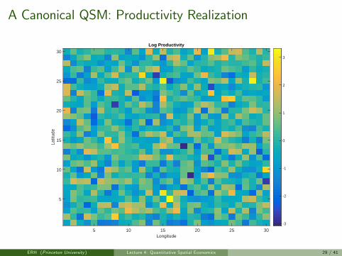
A Canonical QSM: Productivity Realization

Log Productivity

Longitude5 10 15 20 25 30

Latit

ude

5

10

15

20

25

30

-3

-2

-1

0

1

2

3


A Canonical QSM: Parameter Values

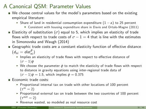
We choose central values for the model’s parameters based on the existingempirical literature:

I Share of land in residential consumption expenditure (1− α) to 25 percentF Consistent with housing expenditure share in Davis and Ortalo-Magne (2011)

Elasticity of substitution (σ) equal to 5, which implies an elasticity of tradeflows with respect to trade costs of σ− 1 = 4 that is line with the estimatesin Simonovska and Waugh (2014)

Trade costs are a constant elasticity function of effective distance(dni = dist

φni )

I Implies an elasticity of trade flows with respect to effective distance of(σ− 1)φ

I We choose the parameter φ to match the elasticity of trade flows with respectto distance in gravity equations using inter-regional trade data of(σ− 1)φ = 1.5, which implies φ = 0.375


A Canonical QSM: Parameter ValuesWe choose central values for the model’s parameters based on the existingempirical literature:

I Share of land in residential consumption expenditure (1− α) to 25 percentF Consistent with housing expenditure share in Davis and Ortalo-Magne (2011)

Elasticity of substitution (σ) equal to 5, which implies an elasticity of tradeflows with respect to trade costs of σ− 1 = 4 that is line with the estimatesin Simonovska and Waugh (2014)Geographic trade costs are a constant elasticity function of effective distance(dni = dist

φni )

I Implies an elasticity of trade flows with respect to effective distance of(σ− 1)φ

I We choose the parameter φ to match the elasticity of trade flows with respectto distance in gravity equations using inter-regional trade data of(σ− 1)φ = 1.5, which implies φ = 0.375

Economic trade costs:I Proportional internal tax on trade with other locations of 100 percent(τin = 2)

I Proportional external tax on trade between the two countries of 100 percent(τout = 2)

I Revenue wasted, so modeled as real resource costERH (Princeton University ) Lecture 4: Quantitative Spatial Economics 31 / 41

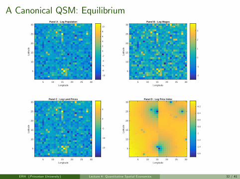
A Canonical QSM: EquilibriumPanel A : Log Population

Longitude5 10 15 20 25 30

Latit

ude

5

10

15

20

25

30

-10

-8

-6

-4

-2

0

2

4

6

8

10

Panel B : Log Wages

Longitude5 10 15 20 25 30

Latit

ude

5

10

15

20

25

30

-2

-1

0

1

2

3

Panel C : Log Land Prices

Longitude5 10 15 20 25 30

Latit

ude

5

10

15

20

25

30

-15

-10

-5

0

5

Panel D : Log Price Index

Longitude5 10 15 20 25 30

Latit

ude

5

10

15

20

25

30

-1.6

-1.4

-1.2

-1

-0.8

-0.6

-0.4

-0.2


A Canonical QSM: External LiberalizationNo tax between countries

Panel A : Log Relative Population

Longitude5 10 15 20 25 30

Latit

ude

5

10

15

20

25

30

0

0.5

1

1.5

2

2.5

3

Panel B : Log Relative Wages

Longitude5 10 15 20 25 30

Latit

ude

5

10

15

20

25

30

-0.1

-0.05

0

0.05

0.1

0.15

0.2

0.25

0.3

Panel C : Log Relative Land Rents

Longitude5 10 15 20 25 30

Latit

ude

5

10

15

20

25

30

0

0.5

1

1.5

2

2.5

3

Panel D : Log Relative Price Index

Longitude5 10 15 20 25 30

Latit

ude

5

10

15

20

25

30

-0.65

-0.6

-0.55

-0.5

-0.45

-0.4

-0.35

-0.3

-0.25

-0.2

-0.15


A Canonical QSM: Internal LiberalizationNo tax between regions

Panel A : Log Relative Population

Longitude5 10 15 20 25 30

Latit

ude

5

10

15

20

25

30

0

0.5

1

1.5

2

2.5

3

3.5

4

Panel B : Log Relative Wages (Truncated)

Longitude5 10 15 20 25 30

Latit

ude

5

10

15

20

25

30

-0.05

-0.04

-0.03

-0.02

-0.01

0

0.01

0.02

0.03

0.04

0.05

Panel C : Log Relative Land Rents

Longitude5 10 15 20 25 30

Latit

ude

5

10

15

20

25

30

-0.5

0

0.5

1

1.5

2

2.5

3

3.5

4

Panel D : Log Relative Price Index (Truncated)

Longitude5 10 15 20 25 30

Latit

ude

5

10

15

20

25

30

-1.35

-1.3

-1.25

-1.2

-1.15


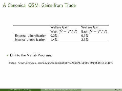
A Canonical QSM: Gains from Trade

Welfare Gain Welfare GainWest (V̂ = V ′/V ) East (V̂ = V ′/V )

External Liberalization 0.2% 0.3%Internal Liberalization 1.4% 2.3%

Link to the Matlab Programs:

https://www.dropbox.com/sh/ujgdq8xx5ki0zfy/AACXqPflODpXt-DXFftNXfEfa?dl=0


https://www.dropbox.com/sh/ujgdq8xx5ki0zfy/AACXqPflODpXt-DXFftNXfEfa?dl=0

Using more Data

General equilibrium spatial models are typically exactly identified

We can still use additional data, assumptions or sources of variation toprovide

I Evidence on the mechanisms in these modelsI Test their quantitative predictions (Over-identification tests)I Structurally estimate their parameters


Market Access

A key implication of quantitative spatial models is that both wages andpopulation depend on market access

Using CES demand, profit maximization and zero profits , the free on boardprice (pi ) charged for each variety by a firm in each location i must be lowenough in order to sell the quantity x̄i and cover the firm’s fixed productioncosts, so (

σ

σ− 1wiAi

)σ

=1x̄i

∑n∈N

(wnLn) (Pn)σ−1 (dni )

1−σ

Define the weighted sum of market demands faced by firms as firm marketaccess (FMAi ) such that

wi = ξAσ−1

σi (FMAi )

1σ , FMAi ≡ ∑

n∈N(wnLn) (Pn)

σ−1 (dni )1−σ

where ξ ≡ (F (σ− 1))−1/σ (σ− 1) /σ collects together earlier constants.

Thus, wages are increasing in both productivity Ai and firm market access(FMAi )


Market Access

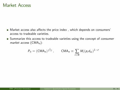
Market access also affects the price index , which depends on consumers’access to tradeable varieties.

Summarize this access to tradeable varieties using the concept of consumermarket access (CMAn):

Pn = (CMAn)11−σ , CMAn ≡ ∑

i∈NMi (pidni )

1−σ


Market Access

Redding and Venables (2004) find a strong correlation between wages andthese measures of market access

For counties within the United States, Hanson (2005) finds a similarly strongrelationship between wages and market access

Establishing that these relationships are causal is more challengingI Typically studies use instrumental variablesI Exclusion restriction that the instruments only affects wages through marketaccess is hard to justify

F Use for example trade liberalizations

Also use changes in transport infrastructure as in Donaldson (2016) forIndia’s railroads and Donaldson and Hornbeck (2016) for U.S. railroads.

Redding and Sturm (2008) use the division of Germany after the SecondWorld War as a natural experiment of changes in market access

I Results are broadly consistent with the model outlined above


Productivity and Density

A large empirical literature finds that wages, land prices, productivity,employment and employment growth are positively correlated with populationdensity

Rosenthal and Strange (2004) report that the elasticity of productivity withrespect to the density of economic activity is typically estimated to lie withinthe range of 3-8 percent

Establishing that this correlation is indeed causal remains challenging

Kline and Moretti (2014) provide evidence on the long-run effects of one ofthe most ambitious regional development programs in U.S. history: theTennessee Valley Authority (TVA)

I Manufacturing employment is found to increase well after federal transfers hadlapsed, consistent with agglomeration economies

Bleakley and Lin (2012) find permanent effects of a temporary historicaladvantage on the spatial distribution of population using variation fromportage sites in the United States


Future Research in QSM

Most research has continued to be concerned with the production and tradeof goods, whereas much economic activity today is concentrated in services,whether tradable or non-tradable

Most of the main frameworks in the literature are static and abstract fromthe effect of spatial frictions on the evolution of the spatial distribution ofeconomic activity and growth

Although there have been several influential studies of the sorting ofheterogeneous workers and firms across geographic space, there remainsscope for further work

The economic analysis of the geography of firm and worker networks remainsunder-explored


lecture 4: quantitative spatial economicserossi/trade/lecture4_552.pdfi in the spirit of the seminal...

Documents