lecture 5: finite differences 1 -...

Lecture 5: Finite differences 1

Sourendu Gupta

TIFR Graduate School

Computational Physics 1February 17, 2010

c©: Sourendu Gupta (TIFR) Lecture 5: Finite differences 1 CP 1 1 / 35

Outline

1 Finite differences

2 Interpolating tabulated values

3 Difference equations

4 Differential equations

5 Function approximationFinite differencesSplinesA first look at Fourier series

6 References


Finite differences

Outline






6 References


Finite differences

The generic function is pathological

The Bolzano-Weierstrass function is defined for any odd positive integer b

as

f (x) =∞

∑

n=0

an cos πbnx , 0 < a < 1, ab > 1 + 3π/2.

This was the first known example of a real function which is continuous atall points, but has no derivative anywhere. Functions of this kind aregeneric. The trajectory of Brownian motion is of this form. Path integralsin any non-trivial field theory are dominated by such paths: they are theessence of quantum theory.

Problem 1: What can you say about the accuracy of numericalcomputations of the BW function and its derivative from the seriesdefinition above? Assume that the machine precision is p. What is thecoarsest grid on which you can tabulate the BW function and still getclose to machine precision evaluation of the function through apolynomial interpolation?


Finite differences

Non-Newtonian machines

The forward, backward and central dif-ferences are

∆hf =f (x + h) − f (x)

h,

∇hf =f (x) − f (x − h)

h,

Dhf =f (x + h) − f (x − h)

2h,

all have the same limit (over reals) as h → 0,and it is the derivative, f ′(x). The limit hasno meaning for floating point numbers: ash becomes smaller and smaller, the differ-ences in the numerator become smaller andcatastrophic loss of significance sets in.

0.000122070312 0.540527344 0.540039062

6.10351562E-05 0.541015625 0.540039062

3.05175781E-05 0.541015625 0.5390625

1.52587891E-05 0.54296875 0.5390625

7.62939453E-06 0.546875 0.5390625

3.81469727E-06 0.546875 0.53125

1.90734863E-06 0.5625 0.53125

9.53674316E-07 0.5625 0.5

4.76837158E-07 0.625 0.5

2.38418579E-07 0.75 0.5

1.19209290E-07 1. 0.5

5.96046448E-08 1. 0.

2.98023224E-08 2. 0.

1.49011612E-08 4. 0.

7.45058060E-09 8. 0.

3.72529030E-09 16. 0.

h, ∆h sin(1.0) and∇h sin(1.0) in singleprecision arithmetic.


Finite differences

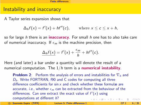
Instability and inaccuracy

A Taylor series expansion shows that

∆hf (x) = f ′(x) + hf ′′(c), where x ≤ c ≤ x + h,

so for large h there is an inaccuracy. For small h one has to also take careof numerical inaccuracy. If ǫm is the machine precision, then

∆hf (x) = f ′(x) +ǫmh

+ hf ′′(c).

Here (and later) a bar under a quantity will denote the result of anumerical computation. The 1/h term is a numerical instability.

Problem 2: Perform the analysis of errors and instabilities for ∇h andDh. Write FORTRAN, f90 and C codes for computing all threedifference coefficients for sin x and check whether these formulæ areaccurate, i.e., whether ǫm can be extracted from the behaviour of thedifferences. Can one extract the exact value of f ′(x) usingcomputations at different h?


Interpolating tabulated values

Outline






6 References



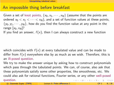
An impossible thing before breakfast

Given a set of knot points, {x0, x1, · · · , xN} (assume that the points areordered x0 < x1 < · · · < xN), and a set of function values at these points,{y0, y1, · · · , yN}, how do you find the function value at any point in therange [x0, xN ]?If you find an answer, f (x), then I can always construct a new function

which coincides with f (x) at every tabulated value and can be made todiffer from f (x) everywhere else by as much as we wish. Therefore, this isan ill-posed question.We try to make the answer unique by asking how to construct polynomialswhich pass through the tabulated points. We can, of course, also ask thatthese polynomials satisfy some other properties, like smoothness, etc. Wecould also ask for rational functions, Fourier series, or any other well-posedquestion.



An impossible thing before breakfast

Given a set of knot points, {x0, x1, · · · , xN} (assume that the points areordered x0 < x1 < · · · < xN), and a set of function values at these points,{y0, y1, · · · , yN}, how do you find the function value at any point in therange [x0, xN ]?If you find an answer, f (x), then I can always construct a new function

f (x) + g(x)N

∏

i=0

(x − xi )

which coincides with f (x) at every tabulated value and can be made todiffer from f (x) everywhere else by as much as we wish. Therefore, this isan ill-posed question.We try to make the answer unique by asking how to construct polynomialswhich pass through the tabulated points. We can, of course, also ask thatthese polynomials satisfy some other properties, like smoothness, etc. Wecould also ask for rational functions, Fourier series, or any other well-posedquestion.



Polynomial fits and van der Monde matrices

Typically, you could find a polynomial of order N which passes throughN + 1 points—

P(x) =N

∑

i=0

cixi , where P(xi ) = yi (0 ≤ i ≤ N).

This gives a set of linear equations to solve—

1 x0 · · · xN0

1 x1 · · · xN1

......

...1 xN · · · xN

N

c0

c1...

cN

=

y0

y1...

yN

.

This (N + 1) × (N + 1) matrix is called a van der Monde matrix. It hasvery small determinant: typically det M ∝ exp[−O(Np)] where p > 1 . Asa result, inverting it by the usual methods leads to catastrophic loss ofprecision. So look for more clever methods.



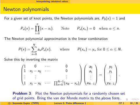
Newton polynomials

For a given set of knot points, the Newton polynomials are, P0(x) = 1 and

Pn(x) =

n∏

i=0

(x − xi ). Note Pn(xα) = 0 when α ≤ n.

The Newton polynomial approximation is the linear combination

P(x) =

N∑

n=0

anPn(x), where P(xα) = yα for 0 ≤ α ≤ N.

Solve this by inverting the matrix

1 0 · · · 01 x1 − x0 · · · 0...

......

1 x1 − x0 · · ·∏N−1

n=0 (xN − xn)

a0

a1

...aN−1

=

y0

y1

...yN−1

.

Problem 3: Plot the Newton polynomials for a randomly chosen setof grid points. Bring the van der Monde matrix to the above form.



Divided differences

Solutions are the divided differences. Solve recursively starting fromequation for a0:

a0 = y0, a1 =y1 − y0

x1 − x0, a2 =

2∑

j=0

yj∏

n=0,2|n 6=j(xj − xn)· · · .

One usually displays this as the tableau:

x0 y0 y(1)0 y

(2)0 y

(3)0 · · ·

x1 y1 y(1)1 y

(2)1 · · ·

x2 y2 y(1)2 · · ·

x3 y3 · · ·

The elements of the tableau can be generated by the recursive formulæ

x(l+1)i = x

(l)i+1 − x

(l)i , y

(l+1)i =

(

y(l)i+1 − y

(l)i

)

/x(l+1)i ,

starting with x(0)i = xi and y

(0)i = yi .



A few problems

Problem 4: Show that when the knot points, xi , approach eachother, the Newton polynomial approximation approaches a truncatedTaylor series. If these computations are performed in floating pointarithmetic, is the limit well-defined? Given a certain machine precision,is there a limit to how closely the xi s can be spaced before catastrophicloss of precision renders the divided differences meaningless?

Problem 5: What relation does the Newton polynomialapproximation bear to the Lagrange interpolation formula

P(t) =

N∑

j=0

yj

∏

n=0,N|n 6=j(t − xn)∏

n=0,N|n 6=j(xj − xn)?

Is there any way to make this approximation behave better than thedivided differences at any fixed value of machine precision?

Problem 6: Are the derivative of the Lagrange interpolation formulacontinuous at the knot points?


Difference equations

Outline






6 References



Solving a finite difference equation

The equation ∆hf = αf gives

f (t + h) = (1 + αh)f (t) = (1 + αh)1+t/hf (0).

In the limit of h → 0, this is indeed the exponential function.With the approximation ∆ for the derivative, we neglect terms of order h2.The solution of the differential equation f ′(t) = αf (t) would give

f (t + h) = ehαf (t) ≃

[

1 + hα + O(h2)]

f (t).

So, the solution of the difference equation is correct to the same order.This will be generalized to Euler’s method. Improvements can beobtained by solving the equation

∆hf =1

h

(

ehα − 1

)

f .

It is common to improve the equation by placing correction terms into theright hand side. It is also possible to use expressions for the derivativewhich are correct to higher order in h.



Instability and inaccuracy

The solution of the differential equation f ′(t) = −αf (t) goes to zero inthe limit t → ∞ for all positive values of α and generic initial conditions.The equation ∆hf = −αf gives

f (t + h) = (1 − αh)f (t) = (1 − αh)1+t/hf (0).

If αh > 2 then |f (t)| → ∞ in the limit t → ∞. In other words, thesolution is unstable.In a region around h = 2/α, one may have catastrophic loss ofsignificance. Even if the loss per step is not catastrophic, errors couldbuild up over many steps. In general, if the error at the n-th step is ǫn,one will have |ǫn| = Kn|ǫ1|, where K is the error in evaluating themultiplicative factor. This is large also when αh is small.If 1 − αh were evaluated exactly, then an error made for some reason atany step of the computation propagates unchanged, i.e., K = 1. Any errorin computing this multiplicative factor increases K . Hence, the error growsexponentially, irrespective of the sign of α.



Stabilizing the solution

One way to stabilize the solution is to replace the difference equation by∆hf (t) = −αf (t + h). Then

f (t + h) =1

1 + αhf (t) =

1

(1 + αh)1+t/hf (0).

This goes to zero in the limit of large t. Since the solution requires theevaluation of the derivative at the next step of the solution, a methodsuch as this is called an implicit method.Another stable solution is obtained by using the difference equation∆hf (t) = −α[f (t) + f (t + h)]/2. This has the solution

f (t + h) =1 − αh/2

1 + αh/2f (t) =

(

1 − αh

1 + αh

)t/h

f (0).

Not only is this stable, one can also check that this is correct to O(h2).Evaluating the derivative at the mid-point of the interval is a techniquewill be used in the 2nd order Runge-Kutta method.



An oscillator: instabilities

The system of equations

df

dt=

(

0 1−1 0

)

f, f(0) =

(

01

)

has the solution f1(t) = sin t and f2(t) = cos t. The corresponding forwarddifference equations, ∆hf(t) = Mf(t), where M is the 2 × 2 matrix above,have the solutions

f(t + h) =

(

1 h

−h 1

)

f(t).

This matrix has eigenvalues λ± = 1 ± ih. Since |λ±| > 1, errors in thecomputed solution will always grow.Replace this by the implicit equation ∆hf(t) = Mf(t + h). Then thesolution is

f(t + h) =

(

1 −h

h 1

)−1

f(t).

This matrix has eigenvalues |λ±| < 1, so the solutions will always decay.c©: Sourendu Gupta (TIFR) Lecture 5: Finite differences 1 CP 1 17 / 35


The leap-frog method0

12

34

56

7

3/2

1/2

5/2

7/2

9/2

11/2

13/2

t= t=The oscillator should have a conserved quantity |f|2. In thesemethods |f(t + h)|2 = |λ±|

2|f(t)|2 = |f(t)|2 + O(h2). If oneimproves the conservation law, one may have a better algo-rithm.Introduce a staggered lattice as here. Place f1 at integerpoints nh and f2 at half-integers (n + 1/2)h. Place the f1 onthe integer lattice and the f2 at the half integer points. Thenthe solutions of the difference equations are—

f1(t + h) = f1(t) + hf2(t +h

2), f2(t +

3h

2) = f2(t +

h

2) − hf1(t + h).

The initial and final half steps are: f2(h/2) = f2(0) − hf1(0)/2 andf2(nh) = f2(nh − h/2) − hf1(nh)/2. Clearly this is equivalent to

f1(t+h) = f1(t)+hf2(t)−h2

2f1(t), f2(t+h) = f2(t)−

h

2[f1(t)+f1(t+h)].

Therefore |f(t + h)|2 = |f(t)|2 + O(h4).c©: Sourendu Gupta (TIFR) Lecture 5: Finite differences 1 CP 1 18 / 35


Using the Euler and leapfrog methods

Problem 7: Write Mathematica functions which will take as inputthe vector f(t) and the quantity h and give back (1) the Euler updatedvector, (2) the implicit Euler updated vector, and (3) the leap-frogupdated vector, f(t + h). In each case use the function to evolve thevector (0, 1)T through time 4π using h = 2π/10, 2π/20, 2π/50 and2π/100. Plot the phase space trajectories, and write out the initial andfinal values of |f|2 in each case.

Problem 8: Generalize the leap-frog method to solve the problem ofthe anharmonic oscillator, i.e.,

H =1

2p2 +

1

4!q4.

Implement your solution in Mathematica and compare it with theresults obtained using the inbuilt methods for solving differentialequations. Change the precision of the Mathematica routines to seehow this affects the solution.


Differential equations

Outline






6 References



Solving differential equations

Euler’s method of solving a system of first order differential equations,f ′(x) = d(f(x), x), is

f(x + h) = f(x) + hd(f(x), x),

where fi (x) is the i − th function. This is equivalent to solving thedifference equation ∆hf(x) = d(f(x), x). The solution is correct to order h.The second-order Runge-Kutta algorithm (RK2) is defined by

f(x+h) = f(x)+hd(f(x+h/2), x+h/2), f(x+h/2) = f(x)+h

2d(f (x), x),

x

RK2

Euler

x+h

x+h/2

f(x) This is correct to O(h2). One can also think ofthis as Euler’s method on a staggered lattice.This corrects the right hand side of the equationby interpolating the derivative linearly between x

and x + h. A quadratic interpolation gives rise tothe fourth order Runge-Kutta algorithm.



Complexity of algorithms

Suppose that the dimension of the vectors f and d is M. Suppose alsothat the CPU time taken to perform an arithmetic operation is T1, andthat required for the evaluation of each component of d is T2. It mayhappen that T2 ≫ T1.Then the time taken per step of the Euler method is M(2T1 +T2), and thetime per step in RK2 is exactly twice, i.e., 2M(2T1 + T2). If the ODEs areintegrated from xi to xf in N steps, i.e., h = (xf − x1)/N, then the timetaken for the Euler method is MN(2T1 + T2), giving an error of O(N−2).RK2 takes exactly twice the time to get an error of O(N−3). A faircomparison would would be of the time taken to make comparable errors.To get an error of O(N−3) using Euler’s method would require time oforder MN3/2(2T1 + T2). We say that RK2 is faster because to get thesame error, the time requirements are

T =

{

O(N3/2) for Euler’s method,

O(N ) for RK2.



Example

Problem 9: The RK2 solution of the equations

dx

dt= v ,

dv

dt= −x ,

are

x(nh +h

2) = x(nh) +

h

2v(nh)

v(nh +h

2) = v(nh) −

h

2x(nh)

x(nh + h) = x(nh) + hv(nh +h

2) =

(

1 −h2

2

)

x(nh) +h

2v(nh)

v(nh + h) = v(nh) − hx(nh +h

2) =

(

1 −h2

2

)

v(nh) −h

2x(nh).

Verify using Mathematica that this is indeed the correct solution ofthe equations upto and including the O(h2) term.



A problem

Problem 10: Implement a leap-frog integration for the anharmonicoscillator

H =1

2p2 +

1

4!q4

as a subroutine in f90 and c which is suitable for updating an ensembleof initial conditions; i.e., it should take a set of (staggered) initial phasespace positions (pi , qi ) where 1 ≤ i ≤ N and a time step, h, and returnthe final phase space positions. Also implement a method for ahalf-step evolution of pi in the beginning and end as a separatesubroutine.

Take N = 1000 different initial conditions distributed uniformly withinthe phase space volume with H ≤ 1. Find the density of points withinthe phase space volumes with H ≤ 1/4, 1/2 and 1. Evolve the systemsusing your program for trajectories of time duration 1, 2, 5 and 10units. At the end of these times compute the same three phase spacedensities as initially. Are these conserved?


Function approximation

Outline






6 References


Function approximation Finite differences

Recursive evaluation of the Lagrange interpolation formula

Let Pi :i+m be the m-th order polynomial interpolating the function at xi ,xi+1, · · · , xi+m. Then one has Neville’s recurrence formula—

Pi :i+m(t) =1

xi+m − xi

∣

∣

∣

∣

t − xi Pi :i+m−1(t)t − xi+m Pi+1:i+m(t)

∣

∣

∣

∣

.

which starts from the constant polynomials Pi :i (t) = yi .If the error in Pi ,i+1,···i+m is δi ,i+1,···i+m, whose magnitude is bounded byδ, then the recurrence gives—

|δi ,i+1,···i+m| ≤ δ

(∣

∣

∣

∣

xi+m − x

xi+m − xi

∣

∣

∣

∣

+

∣

∣

∣

∣

x − xi

xi+m − xi

∣

∣

∣

∣

)

= δ.

Therefore errors in the function values do not grow unless the knot pointsare so close that terms like xi+m − xi are dominated by catastrophic loss ofsignificance.For a further improvement on this algorithm, see Numerical Recipes.



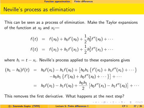
Neville’s process as elimination

This can be seen as a process of elimination. Make the Taylor expansionsof the function at x0 and x1—

f (t) = f (x0) + h0f′(x0) +

1

2h20f

′′(x0) + · · ·

f (t) = f (x1) + h1f′(x1) +

1

2h21f

′′(x1) + · · ·

where hi = t − xi . Neville’s process applied to these expansions gives

(h1 − h0)f (t) = h0f (x1) − h1f (x0) +[

h0h1

{

f ′(x1) + h1f′′(x1) + · · ·

}

−h0h1

{

f ′(x0) + h0f′′(x0) + · · ·

}]

+ · · ·

= h0f (x1) − h1f (x0) +h0h1

2

[

h0f′′(x1) − h1f

′′(x0)]

+ · · ·

This removes the first derivative. What happens at the next step?



Is Lagrange interpolation a well-posed problem?

Problem 11: Write a Mathematica code which starts from a Taylorexpansion of a function (and its derivatives) around some number ofknot points. Apply successive steps of Neville’s process to this andshow that at each step of the process one more derivative is removed.

Problem 12: We have shown above that initial errors, δ, in thefunction values, yi , do not grow when using Lagrange interpolationusing Neville’s recurrence. Check what happens to the Newtonpolynomials, divided differences, the Lagrange interpolation formulaand Neville’s recurrence when the knot point, xi , are changed slightly.What happens when one of the knot-points is removed entirely? Is thebehaviour equally stable (or unstable) for interpolation (i.e.,x0 ≤ t ≤ xN) and extrapolation (t < x0 or t > xN)?



Numerical integration

Problem 13: Given a polynomial approximation to tabulated data onfunctions, give expressions for integrating them. Note that theintegration formulae should only involve the tabulated function valuesand constants. Read the Newton-Cotes integration formulae and checkwhat kind of function interpolations they come from.

Problem 14: Consider integrals of functions with poles in the regionof integration, such as

I =

∫ ∞

−∞

dxP(x)

x − 1,

where P(1) 6= 0. These are often regularized using the CauchyPrincipal Value prescription—

I =Lim

ǫ → 0

∫ 1−ǫ

−∞

dxP(x)

x − 1+

∫ ∞

1+ǫ

dxP(x)

x − 1.

Find an efficient method of evaluating the principal value. How doesthe value change if the integral is defined as the sum over the the twointervals [−∞, 1 − 5ǫ] and [1 + ǫ,∞]?


Function approximation Splines

Smooth polynomials

Given knot points {x0, x1} and function values {y0, y1}, one has a linearinterpolation

g(t) = A(t)y0+B(t)y1, where A(t) =t − x1

x0 − x1, B(t) =

x0 − t

x0 − x1.

The first derivative is constant in the interval (x0, x1). In the next interval,(x1, x2), the first derivative is again constant but a different value. As aresult, the second derivative is discontinuous at the knot points.If one had information on the second derivatives at the knot points, onecould build an interpolating function

h(t) = A(t)y ′′0 + B(t)y ′′

1 .

Using this, one could try to make cubic interpolating function

f (t) = g(t) + (t − x0)(t − x1)h(t),

and arrange it to have continuous first derivatives at the knot points. Thisis the idea of a spline.


Function approximation Splines

Cubic splines

In fact the first derivative is

f ′(t) = g ′(t)y1 + (t − x0 + t − x1)h(t) + (t − x0)(t − x1)h′(t).

At the knot point x1 one has the two expressions—

f ′(x1) =y0 − y1

x0 − x1− (x0 − x1)y

′′1 , f ′(x1) =

y1 − y2

x1 − x2+ (x1 − x2)y

′′1 .

Continuity of the derivative is obtained by equating these two expressions.This gives a solution for the unknown quantity—

y ′′1 =

1

x0 − x2

[

y0 − y1

x0 − x1−

y1 − y2

x1 − x2

]

.

One can eliminate y ′′i at every knot point except x0 and xN . At these two

points one can give a boundary condition of one’s choice.


Function approximation A first look at Fourier series

A Fourier series

A periodic function y(t) = y(t + L), has a compact representation as theFourier series

y(t) =

N∑

k=0

fk exp

(

2πitk

NL

)

.

The Fourier coefficients are given by the solution of a complex van derMonde matrix equation

1 z0 · · · zN0

1 z1 · · · zN1

......

...1 zN · · · zN

N

f0f1...

fN

=

y0

y1...

yN

.

where zj = exp(2πixj/NL) and |zj | = 1. If the knot points xj = jL, thenthe zjs are roots of unity, and the sum over the elements of all but one rowadd up to zero. Since the rows orthogonal to each other, the matrix isinvertible.


Function approximation A first look at Fourier series

Fourier inversion

In fact, the definition of the Fourier transformation,

fk =1

N + 1

N∑

j=0

yj exp

(

−2πixjk

NL

)

,

gives the inverse (z∗j is the complex conjugate of zj)

1

N + 1

1 1 · · · 1z∗0 z∗1 · · · z∗N...

......

z∗0N z∗1

N · · · z∗NN

y0

y1...

yN

=

f0f1...

fN

.

Problem 15: Hadamard’s bound states that for a real(N + 1) × (N + 1) matrix whose elements are bounded by unity, thedeterminant is at most (N + 1)(N+1)/2. What relation do the Fouriermatrices hold to Hadamard matrices, i.e., those real matrices whichsatisfy the bound?


References

Outline






6 References


References

References and further reading

1 Numerical Recipes, by W. H. Press, S. A. Teukolsky, W. T.Vetterling, B. P. Flannery, Cambridge University Press. Treat this asa well written manual for a ready source of building blocks. However,be ready to go into the blocks to improve their performance.

2 E. H. Neville, “Iterative interpolation”, Journal of the Indian

Mathematical Society , Vol 20, p. 87 (1934).

3 Several points in this lecture are illustrated in the associatedMathematica notebooks. These notebooks also have additionalexamples. They are given in tar.gz format. Unpack them using thetar -xvzf command.


http://theory.tifr.res.in/~sgupta/courses/cp2010/Math/lec5.tar.gz

lecture 5: finite differences 1 -...

Documents