lecture # 5 spatial filteringbiomisa.org/wp-content/uploads/2019/02/lect-5.pdf · smoothing spatial...
TRANSCRIPT
1
Digital Image Processing
Lecture # 5Spatial Filtering
Spatial Filtering

3
Spatial Filtering
4
Spatial Filtering
5
Spatial Filtering

6
Spatial Filtering

Spatial Filtering
8
Spatial Filtering: Basics
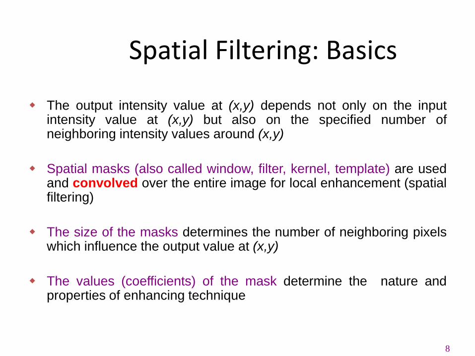
The output intensity value at (x,y) depends not only on the inputintensity value at (x,y) but also on the specified number ofneighboring intensity values around (x,y)
Spatial masks (also called window, filter, kernel, template) are usedand convolved over the entire image for local enhancement (spatialfiltering)
The size of the masks determines the number of neighboring pixelswhich influence the output value at (x,y)
The values (coefficients) of the mask determine the nature andproperties of enhancing technique

9
Spatial Filtering: Basics
1 1where a = , b =
2 2
0,1,2,...., 1, 0,1,2,..., 1
m n
x M y N
( , ) ( , ) ( , )a b
s a t b
g x y w s t f x s y t
Filtering can be given in equation
form as shown above
10
Spatial Filtering: Basics
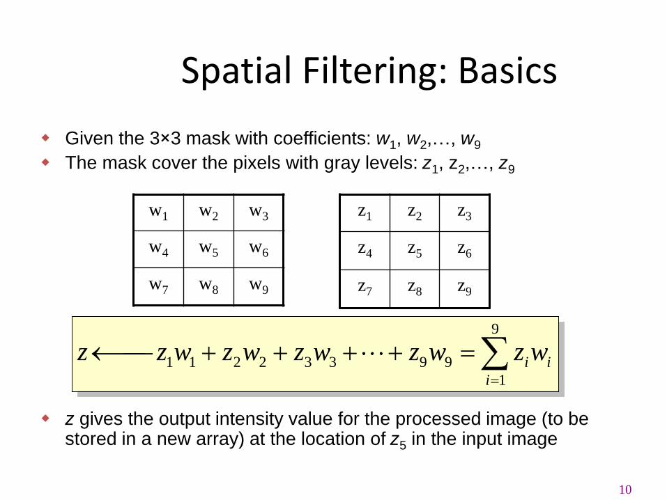
Given the 3×3 mask with coefficients: w1, w2,…, w9
The mask cover the pixels with gray levels: z1, z2,…, z9
z gives the output intensity value for the processed image (to be stored in a new array) at the location of z5 in the input image
z1 z2 z3
z4 z5 z6
z7 z8 z9
9
1 1 2 2 3 3 9 9
1
i i
i
z z w z w z w z w z w
w1 w2 w3
w4 w5 w6
w7 w8 w9
13
Spatial Filtering: Basics
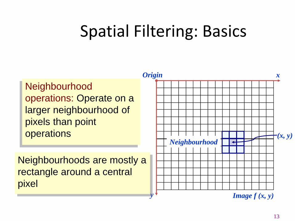
Neighbourhood
operations: Operate on a
larger neighbourhood of
pixels than point
operations
Origin x
y Image f (x, y)
(x, y)Neighbourhood
Neighbourhoods are mostly a
rectangle around a central
pixel
14
Spatial Filtering: Basics
r s t
u v w
x y z
Origin x
y Image f (x, y)
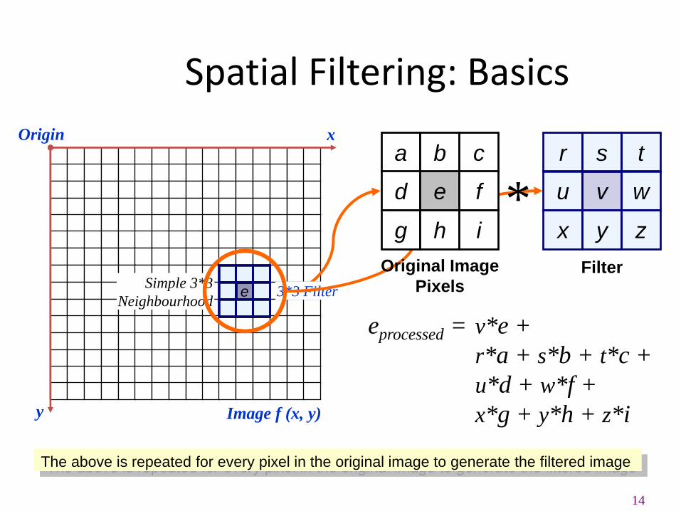
eprocessed = v*e +
r*a + s*b + t*c +
u*d + w*f +
x*g + y*h + z*i
FilterSimple 3*3
Neighbourhoode 3*3 Filter
a b c
d e f
g h i
Original Image
Pixels
*
The above is repeated for every pixel in the original image to generate the filtered image
15
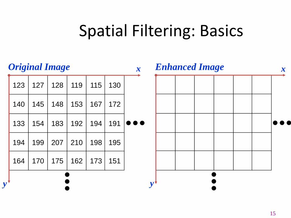
Spatial Filtering: Basics
123 127 128 119 115 130
140 145 148 153 167 172
133 154 183 192 194 191
194 199 207 210 198 195
164 170 175 162 173 151
Original Image x
y
Enhanced Image x
y

16
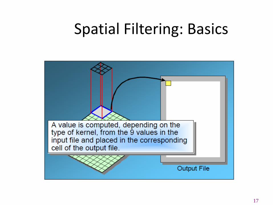
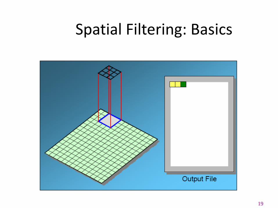
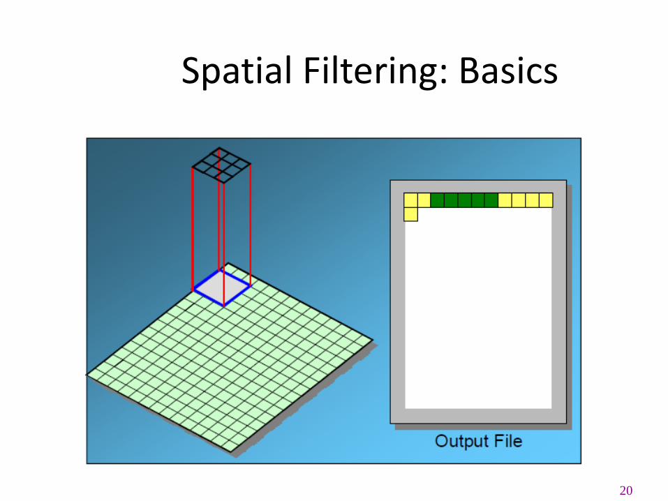
Spatial Filtering: Basics
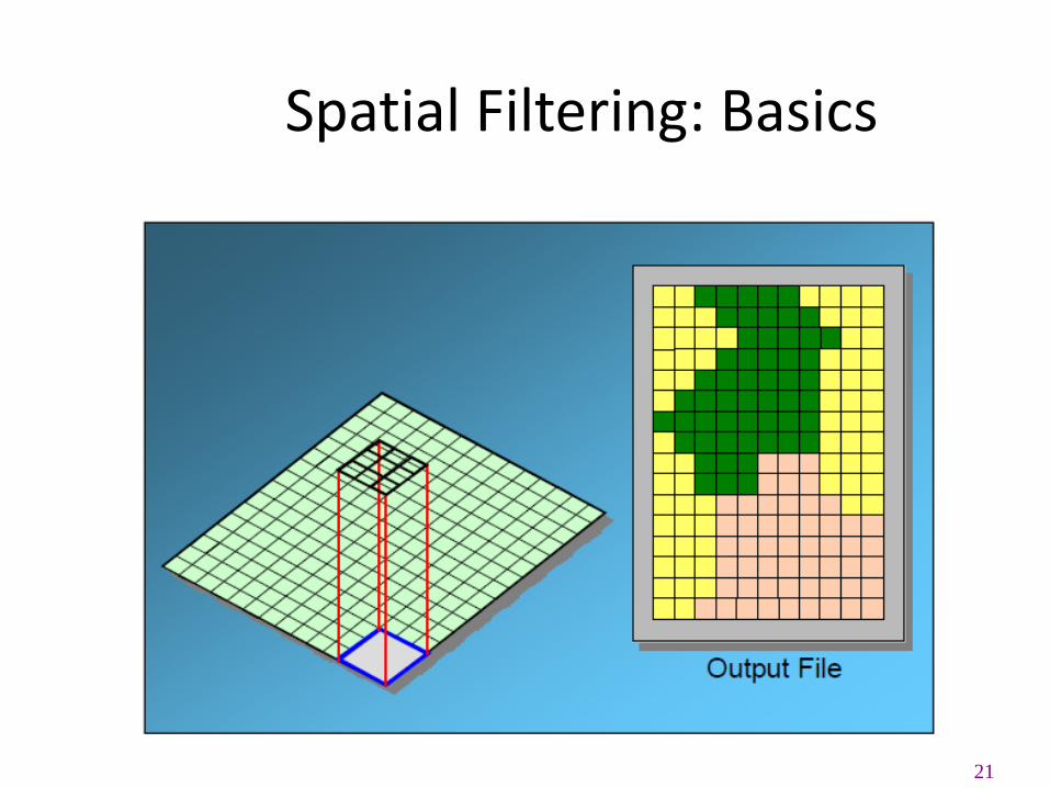
Moving window (kernel)
scans the 3x3
neighborhood of every
pixel in the image
Original Image
17
Spatial Filtering: Basics

18
Spatial Filtering: Basics
19
Spatial Filtering: Basics
20
Spatial Filtering: Basics
21
Spatial Filtering: Basics
22
Spatial Filtering: Basics
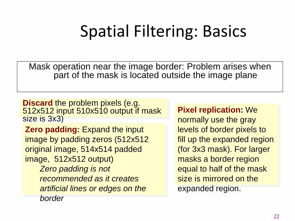
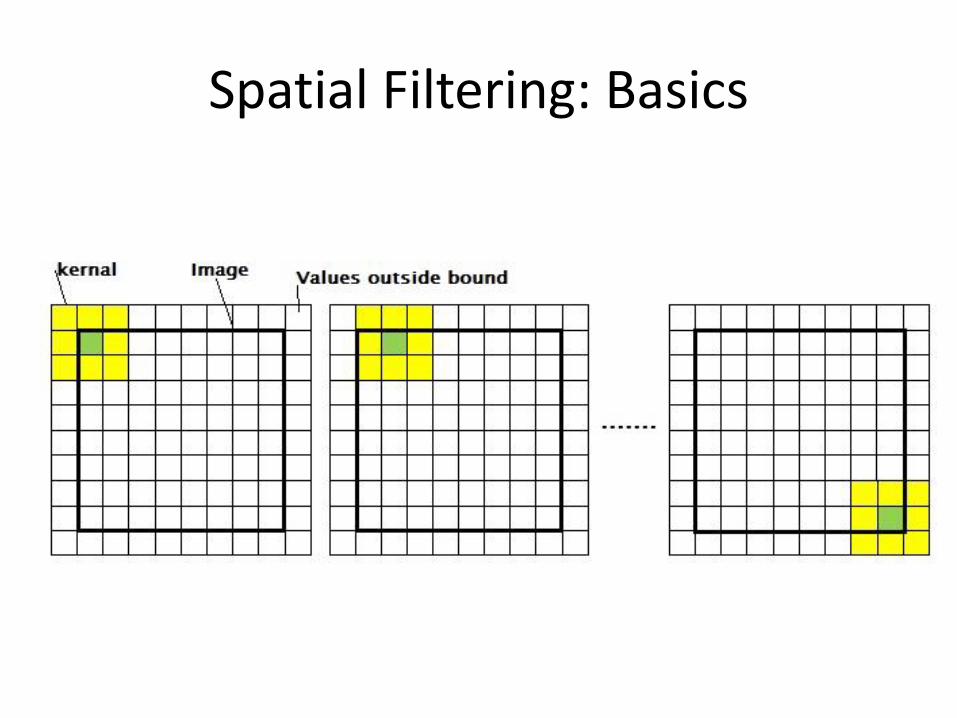
Mask operation near the image border: Problem arises when part of the mask is located outside the image plane
Discard the problem pixels (e.g. 512x512 input 510x510 output if mask size is 3x3)
Zero padding: Expand the input
image by padding zeros (512x512
original image, 514x514 padded
image, 512x512 output)
Zero padding is not
recommended as it creates
artificial lines or edges on the
border
Pixel replication: We
normally use the gray
levels of border pixels to
fill up the expanded region
(for 3x3 mask). For larger
masks a border region
equal to half of the mask
size is mirrored on the
expanded region.
Spatial Filtering: Basics

24
Mask operation near the border: Pixel replication
25
Smoothing Spatial Filters
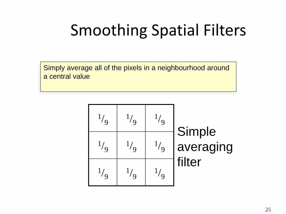
Simply average all of the pixels in a neighbourhood around
a central value
1/91/9
1/9
1/91/9
1/9
1/91/9
1/9
Simple
averaging
filter
26
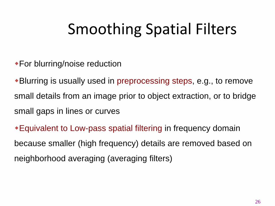
Smoothing Spatial Filters
For blurring/noise reduction
Blurring is usually used in preprocessing steps, e.g., to remove
small details from an image prior to object extraction, or to bridge
small gaps in lines or curves
Equivalent to Low-pass spatial filtering in frequency domain
because smaller (high frequency) details are removed based on
neighborhood averaging (averaging filters)
27
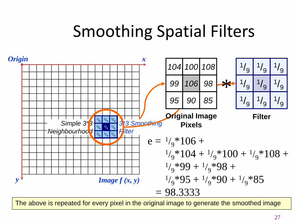
Smoothing Spatial Filters
1/91/9
1/91/9
1/91/9
1/91/9
1/9
Origin x
y Image f (x, y)
e = 1/9*106 + 1/9*104 + 1/9*100 + 1/9*108 + 1/9*99 + 1/9*98 + 1/9*95 + 1/9*90 + 1/9*85
= 98.3333
FilterSimple 3*3
Neighbourhood106
104
99
95
100 108
98
90 85
1/91/9
1/9
1/91/9
1/9
1/91/9
1/9
3*3 Smoothing
Filter
104 100 108
99 106 98
95 90 85
Original Image
Pixels
*
The above is repeated for every pixel in the original image to generate the smoothed image

28
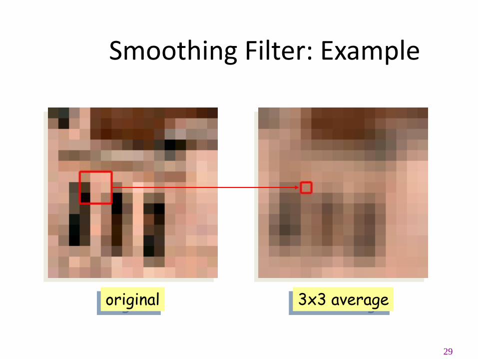
Smoothing Filter: Example
original 3x3 average
29
Smoothing Filter: Example
original 3x3 average

30
Smoothing Filter: Example
original 3x3 average

31
Smoothing Filter: Example
original 3x3 average
32
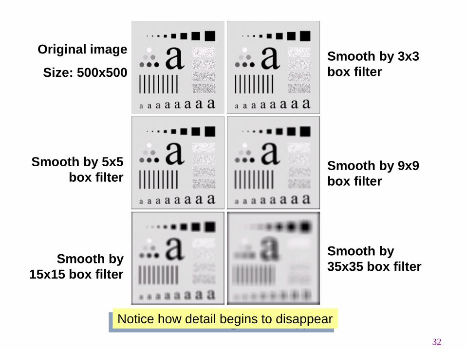
Original image
Size: 500x500
Smooth by 3x3
box filter
Smooth by 5x5
box filterSmooth by 9x9
box filter
Smooth by
15x15 box filter
Smooth by
35x35 box filter
Notice how detail begins to disappear
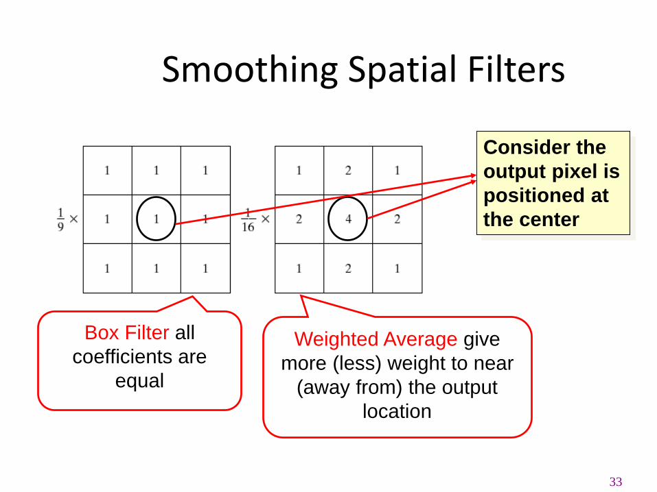
33
Smoothing Spatial Filters
Box Filter all
coefficients are
equal
Weighted Average give
more (less) weight to near
(away from) the output
location
Consider the
output pixel is
positioned at
the center
Sharpening Spatial Filters
Previously we have looked at smoothing filters which remove
fine detail
Sharpening spatial filters seek to highlight fine detail
Remove blurring from images
Highlight edges
Sharpening filters are based on spatial differentiation
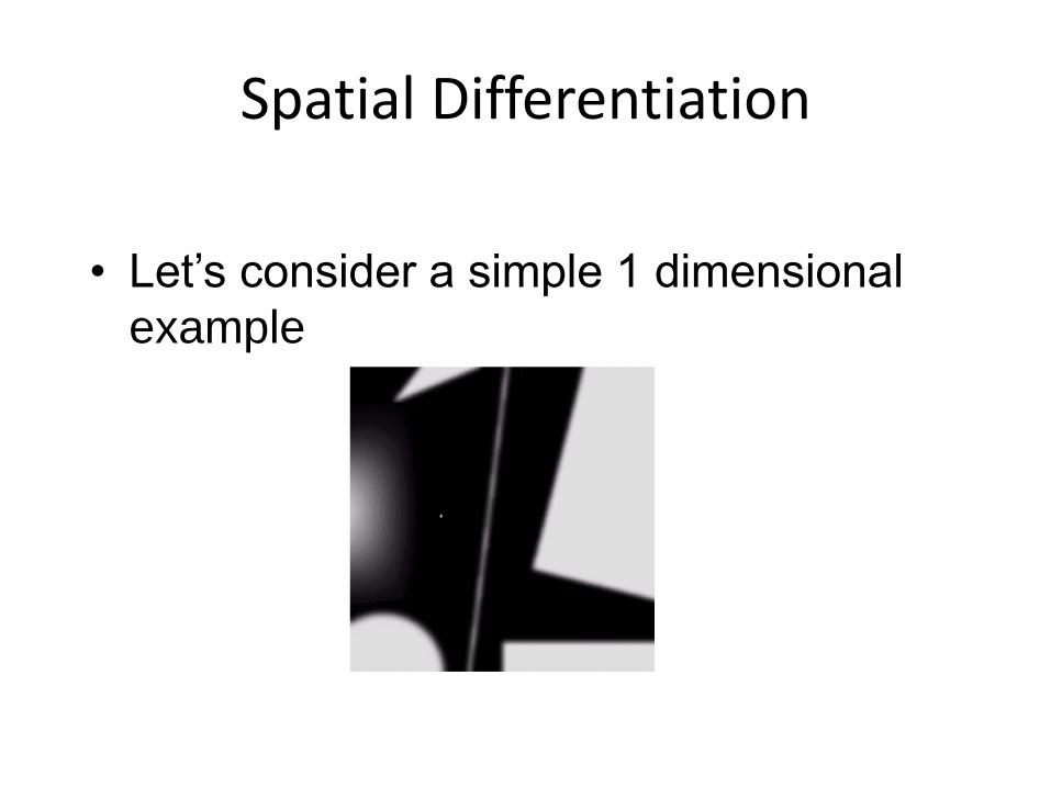
Spatial Differentiation
• Let’s consider a simple 1 dimensional
example
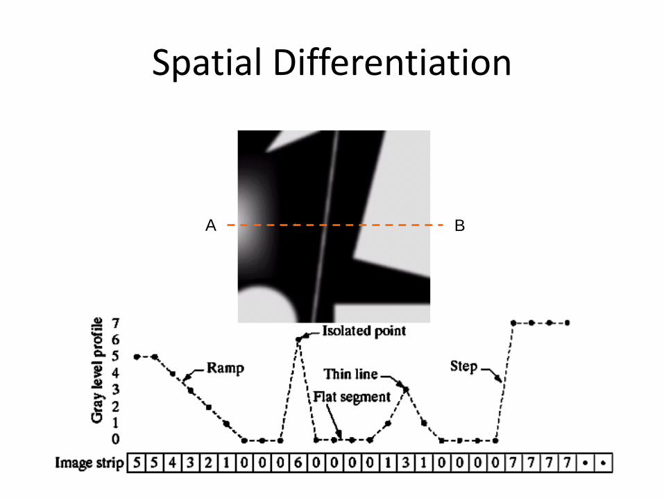
Spatial Differentiation
A B
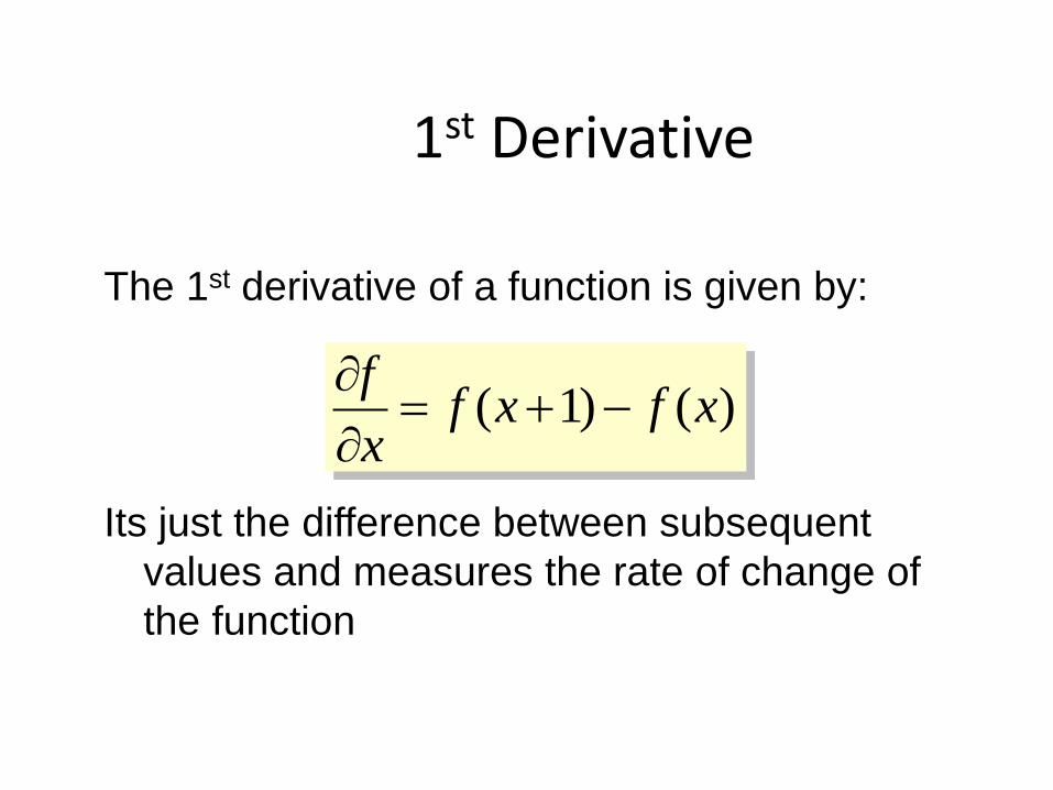
1st Derivative
The 1st derivative of a function is given by:
Its just the difference between subsequent
values and measures the rate of change of
the function
)()1( xfxfx
f

Image Strip
0
1
2
3
4
5
6
7
8
1st Derivative
-8
-6
-4
-2
0
2
4
6
8
5 5 4 3 2 1 0 0 0 6 0 0 0 0 1 3 1 0 0 0 0 7 7 7 7
-1 -1 -1 -1 -1 0 0 6 -6 0 0 0 1 2 -2 -1 0 0 0 7 0 0 0
1st Derivative
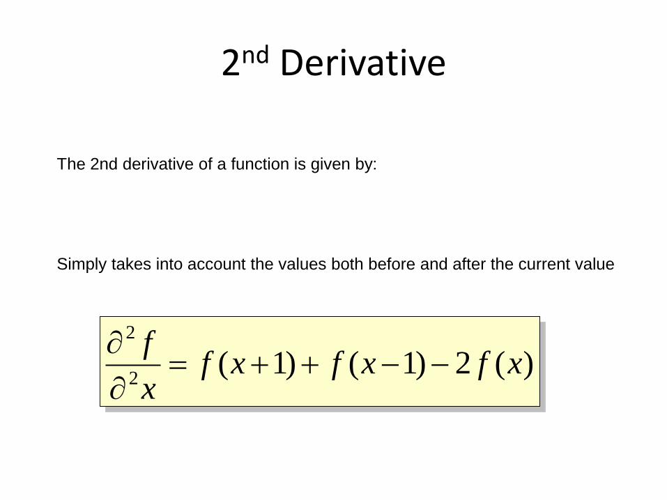
2nd Derivative
The 2nd derivative of a function is given by:
Simply takes into account the values both before and after the current value
)(2)1()1(2
2
xfxfxfx
f

Image Strip
0
1
2
3
4
5
6
7
8
5 5 4 3 2 1 0 0 0 6 0 0 0 0 1 3 1 0 0 0 0 7 7 7 7
2nd Derivative
2nd Derivative
-15
-10
-5
0
5
10
-1 0 0 0 0 1 0 6 -12 6 0 0 1 1 -4 1 1 0 0 7 -7 0 0
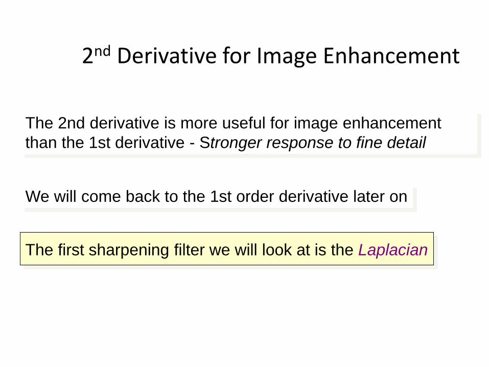
2nd Derivative for Image Enhancement
The 2nd derivative is more useful for image enhancement
than the 1st derivative - Stronger response to fine detail
We will come back to the 1st order derivative later on
The first sharpening filter we will look at is the Laplacian
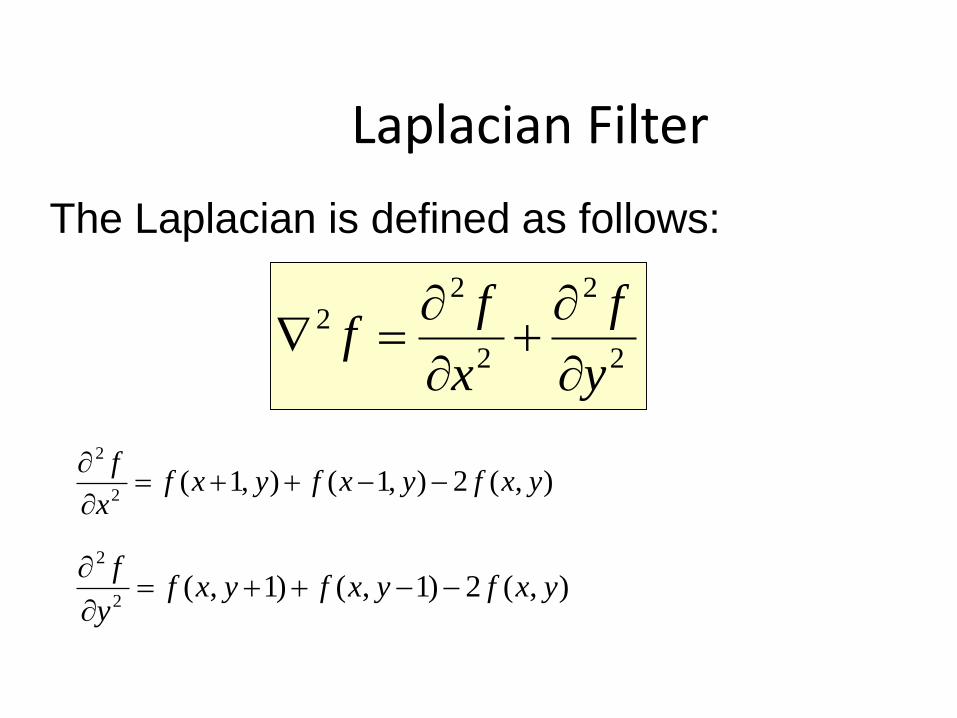
Laplacian Filter
2
2
2
22
y
f
x
ff
),(2),1(),1(2
2
yxfyxfyxfx
f
The Laplacian is defined as follows:
),(2)1,()1,(2
2
yxfyxfyxfy
f

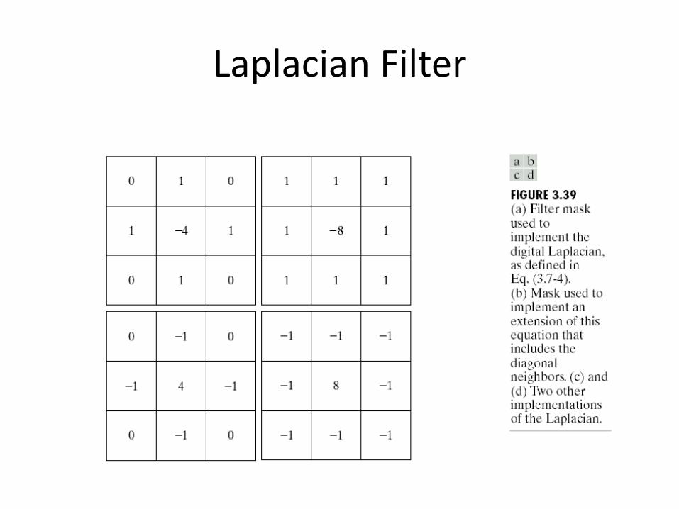
Laplacian Filter
So, the Laplacian can be given as follows:
),1(),1([2 yxfyxff
)]1,()1,( yxfyxf
),(4 yxf
0 1 0
1 -4 1
0 1 0
Can we implement it using a filter/ mask?
Laplacian Filter
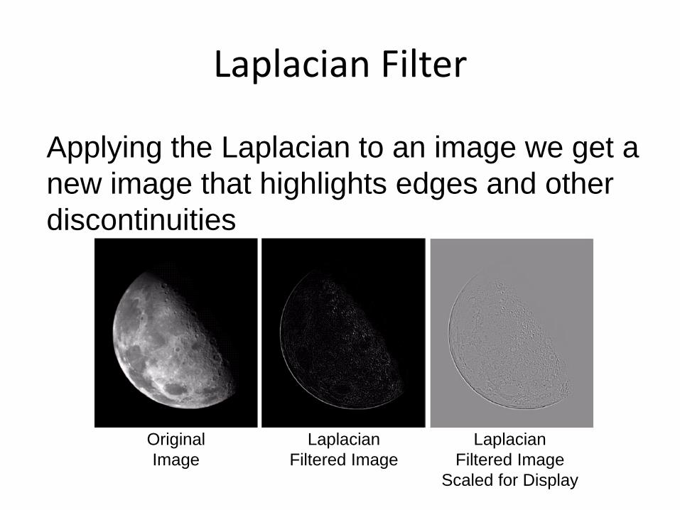
Laplacian Filter
Applying the Laplacian to an image we get a
new image that highlights edges and other
discontinuities
Original
Image
Laplacian
Filtered Image
Laplacian
Filtered Image
Scaled for Display
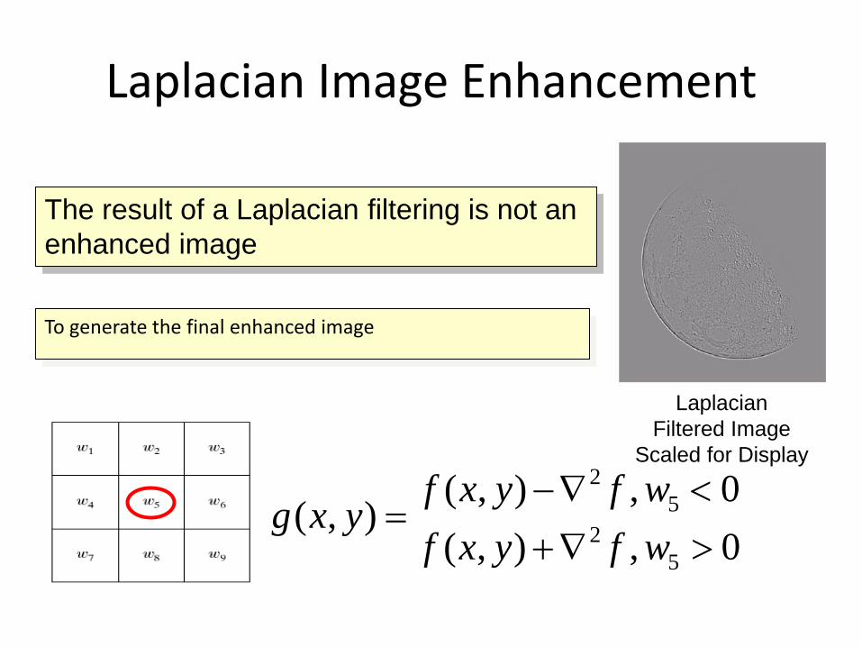
Laplacian Image Enhancement
The result of a Laplacian filtering is not an
enhanced image
Laplacian
Filtered Image
Scaled for Display2
5
2
5
( , ) , 0( , )
( , ) , 0
f x y f wg x y
f x y f w
To generate the final enhanced image
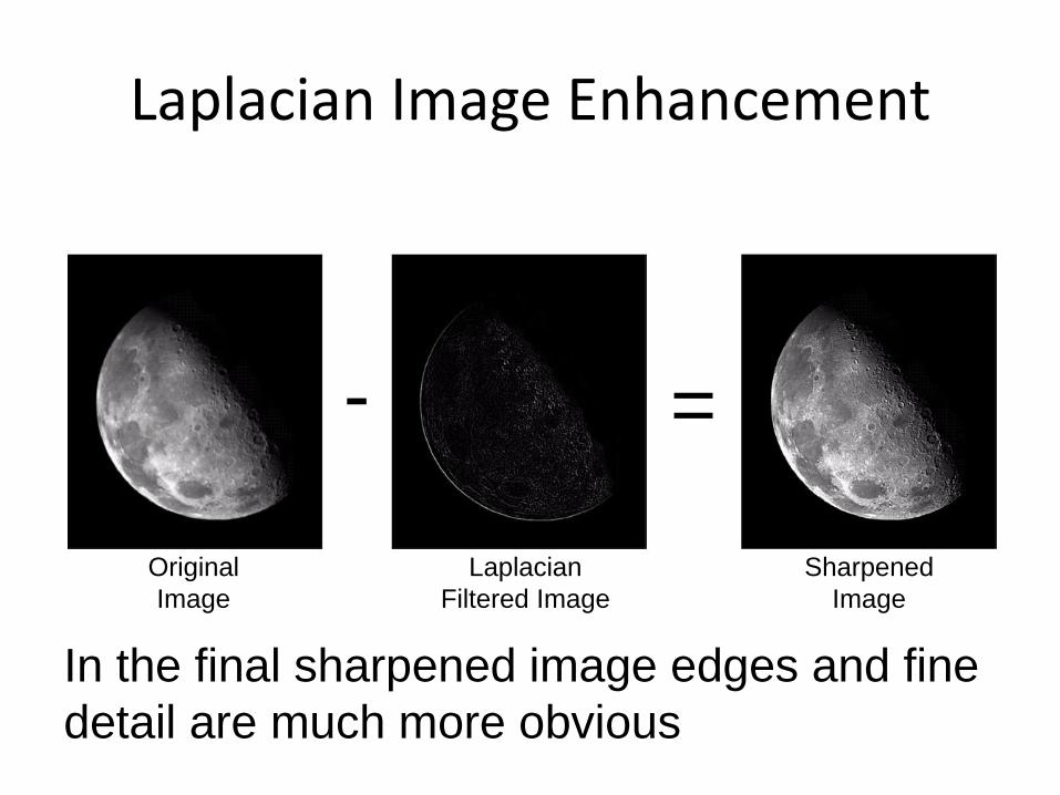
Laplacian Image Enhancement
In the final sharpened image edges and fine
detail are much more obvious
- =
Original
Image
Laplacian
Filtered Image
Sharpened
Image

Laplacian Image Enhancement
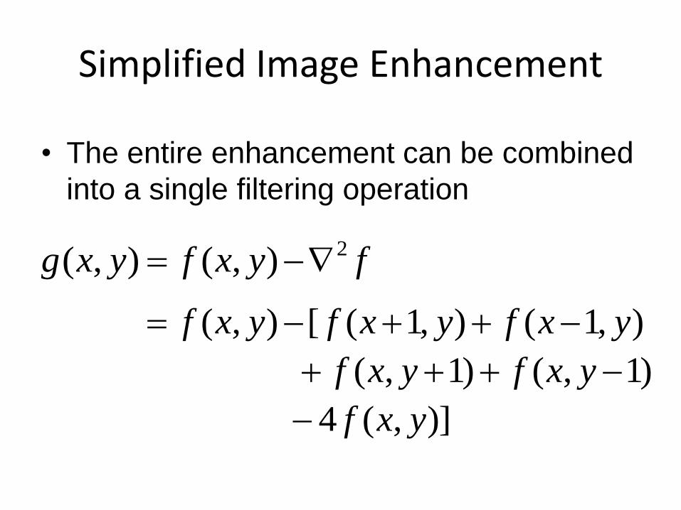
Simplified Image Enhancement
• The entire enhancement can be combined
into a single filtering operation
),1(),1([),( yxfyxfyxf
)1,()1,( yxfyxf
)],(4 yxf
fyxfyxg 2),(),(
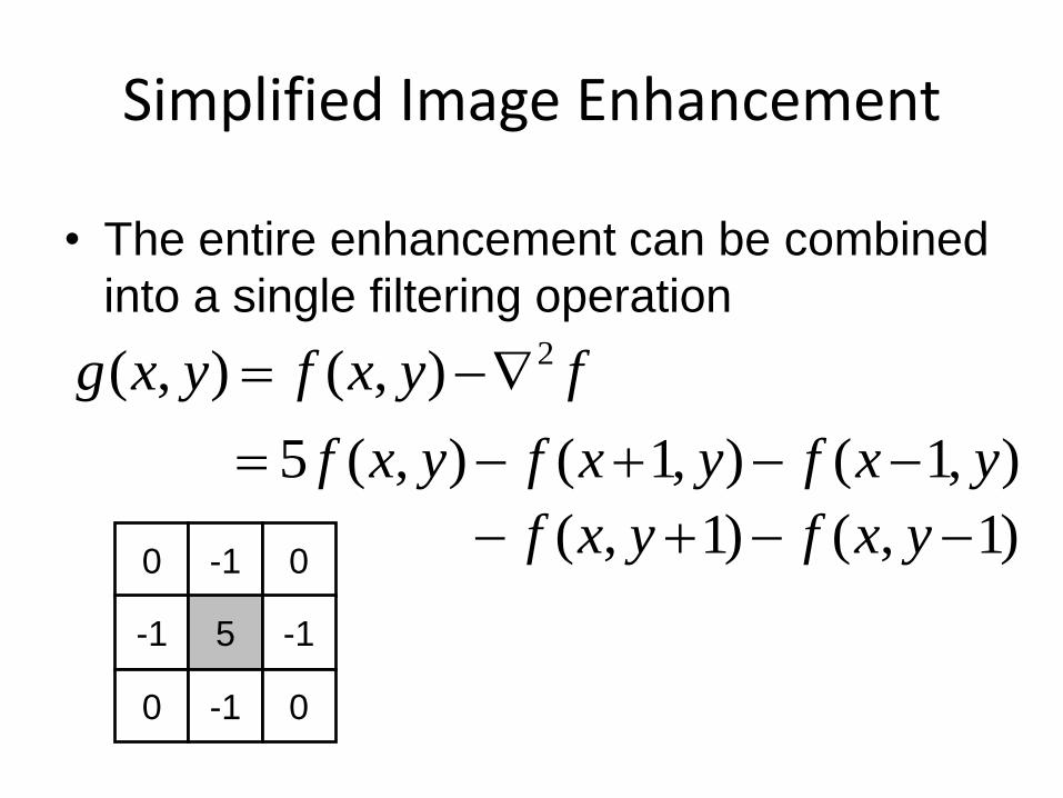
Simplified Image Enhancement
• The entire enhancement can be combined
into a single filtering operation
fyxfyxg 2),(),(
),1(),1(),(5 yxfyxfyxf
)1,()1,( yxfyxf0 -1 0
-1 5 -1
0 -1 0
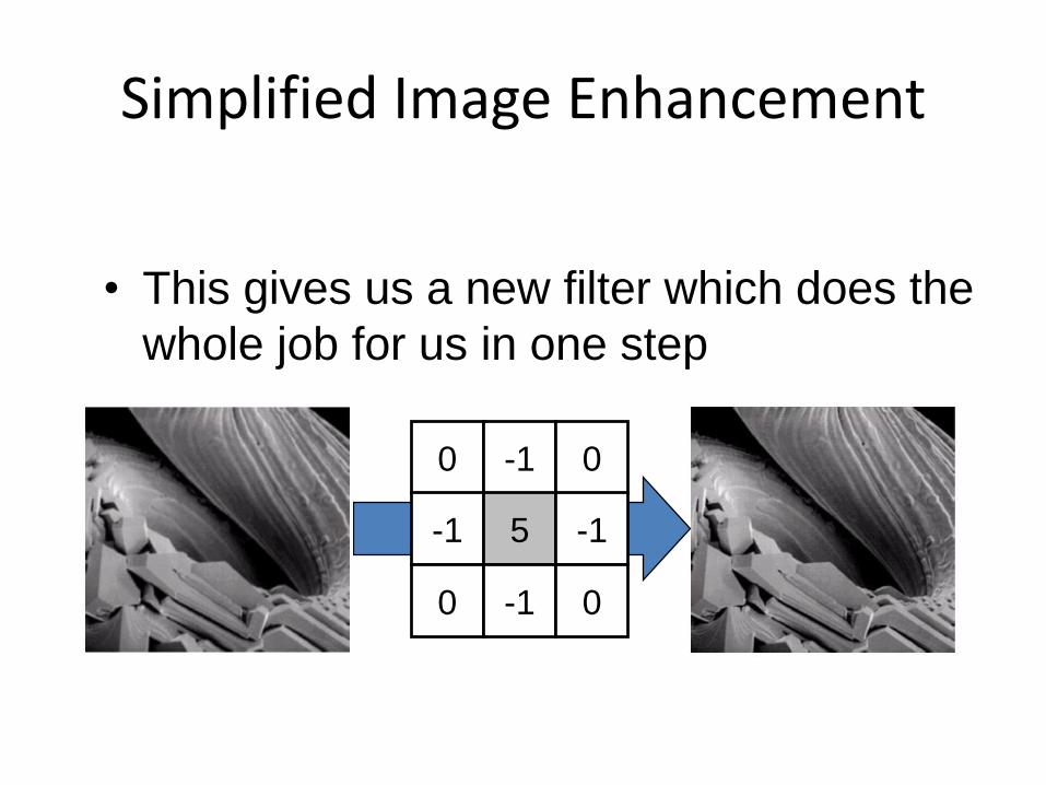
Simplified Image Enhancement
• This gives us a new filter which does the
whole job for us in one step
0 -1 0
-1 5 -1
0 -1 0
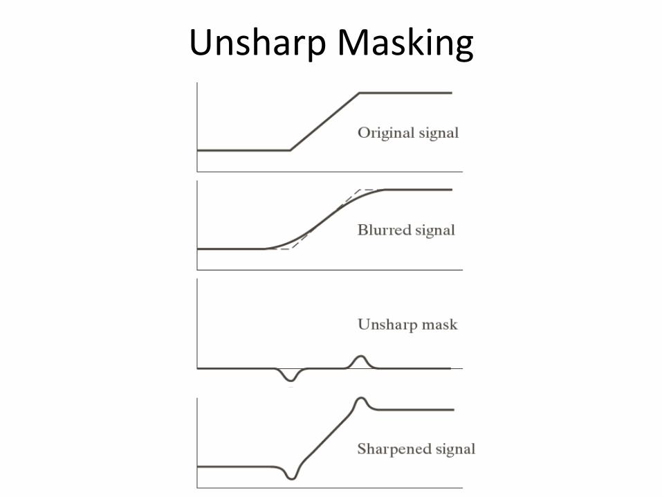
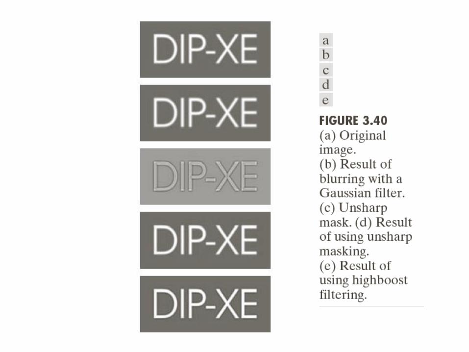
Unsharp Masking

Use of first derivatives for image enhancement: The Gradient
• The gradient of a function f(x,y) is defined as
y
fx
f
G
G
y
xf
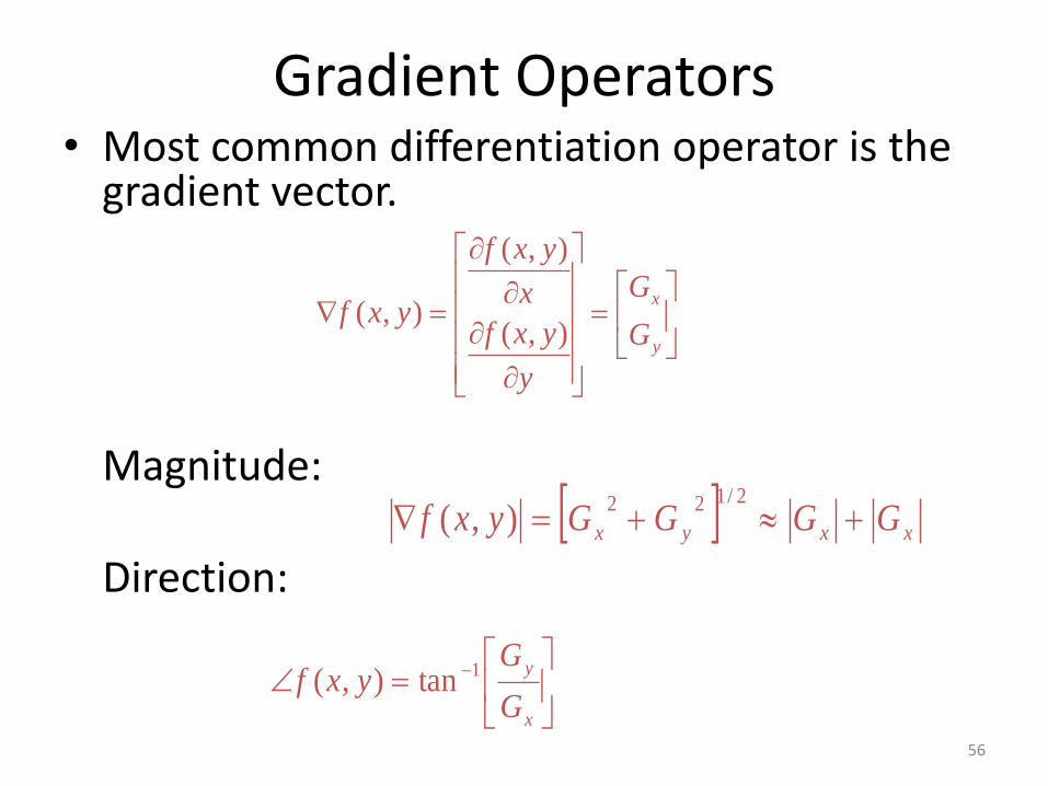
Gradient Operators• Most common differentiation operator is the
gradient vector.
Magnitude:
Direction:
y
x
G
G
y
yxf
x
yxf
yxf),(
),(
),(
xxyx GGGGyxf 2/122
),(
x
y
G
Gyxf 1tan),(
56
-1 -2 -1
0 0 0
1 2 1
-1 0 1
-2 0 2
-1 0 1
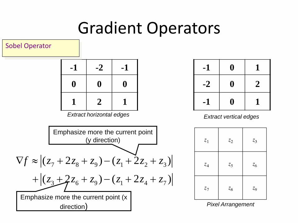
Extract horizontal edges
7 8 9 1 2 3
3 6 9 1 4 7
( 2 ) ( 2 )
( 2 ) ( 2 )
f z z z z z z
z z z z z z
Emphasize more the current point
(y direction)
Emphasize more the current point (x
direction) Pixel Arrangement
Gradient Operators
Extract vertical edges
Sobel Operator
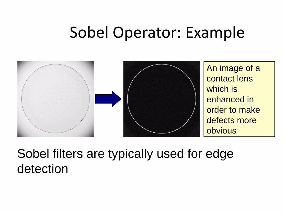
Sobel Operator: Example
Sobel filters are typically used for edge
detection
An image of a
contact lens
which is
enhanced in
order to make
defects more
obvious
59
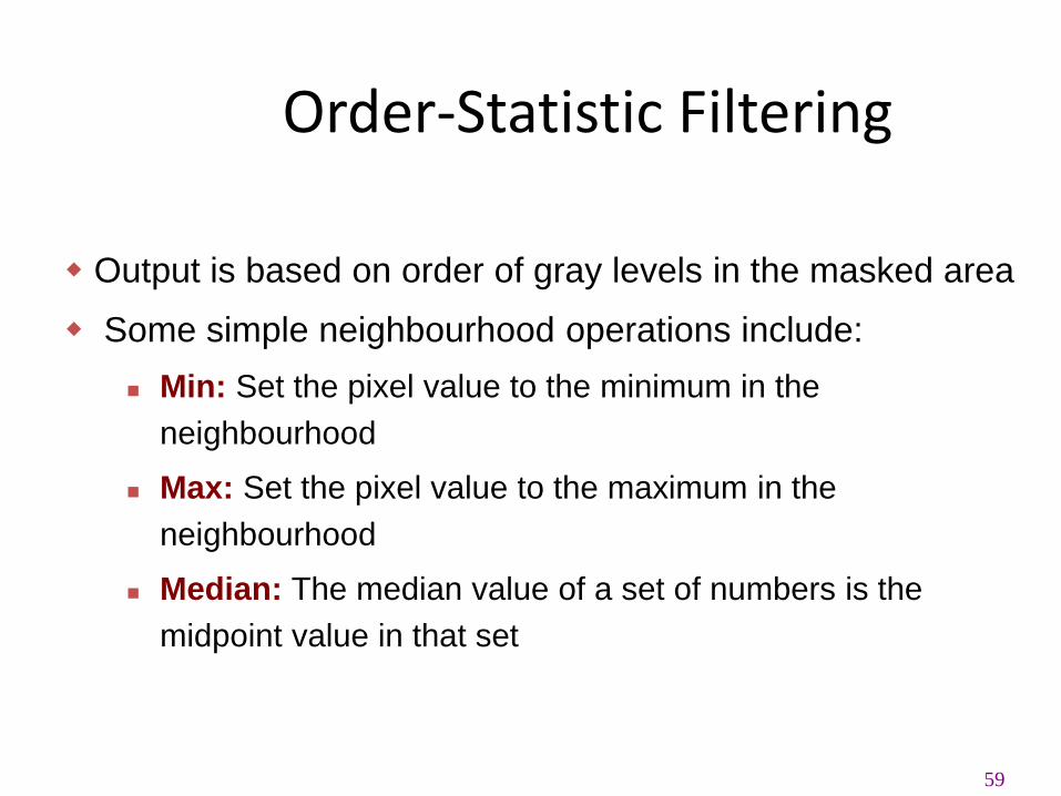
Order-Statistic Filtering
Output is based on order of gray levels in the masked area
Some simple neighbourhood operations include:
Min: Set the pixel value to the minimum in the
neighbourhood
Max: Set the pixel value to the maximum in the
neighbourhood
Median: The median value of a set of numbers is the
midpoint value in that set
60
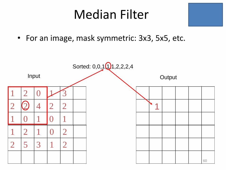
Median Filter
• For an image, mask symmetric: 3x3, 5x5, etc.
0 2
1 2
1 2 1
2 5 3
1 3
2 2
0 1
1 2 0
2 2 4
1 0 1
Input Output
Sorted: 0,0,1,1,1,2,2,2,4
1

61
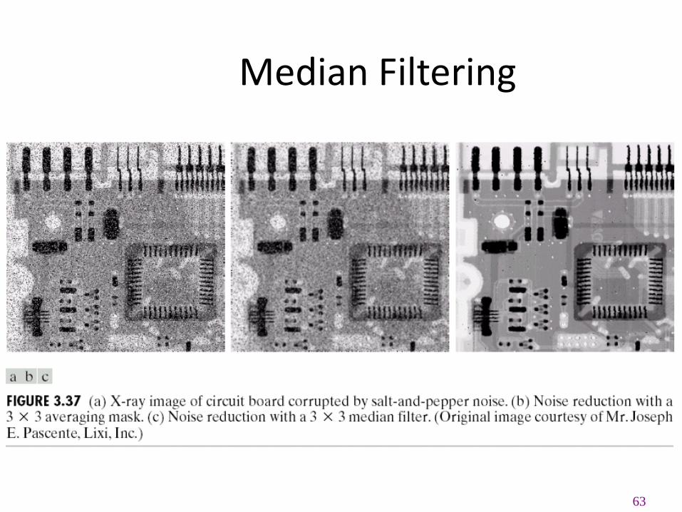
Median Filtering
Median = ? 20
Particularly effective when
The noise pattern consists of strong
impulse noise ( salt-and-pepper)
Sort the values
Determine the median

Salt and Pepper Noise
63
Median Filtering

Min/Max Filtering
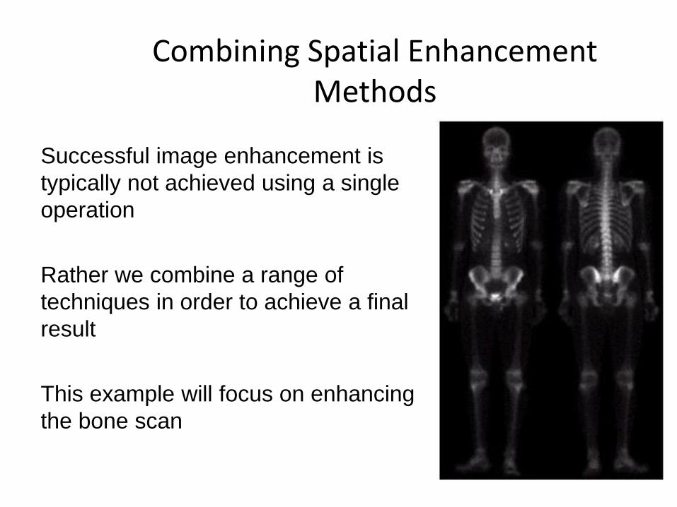
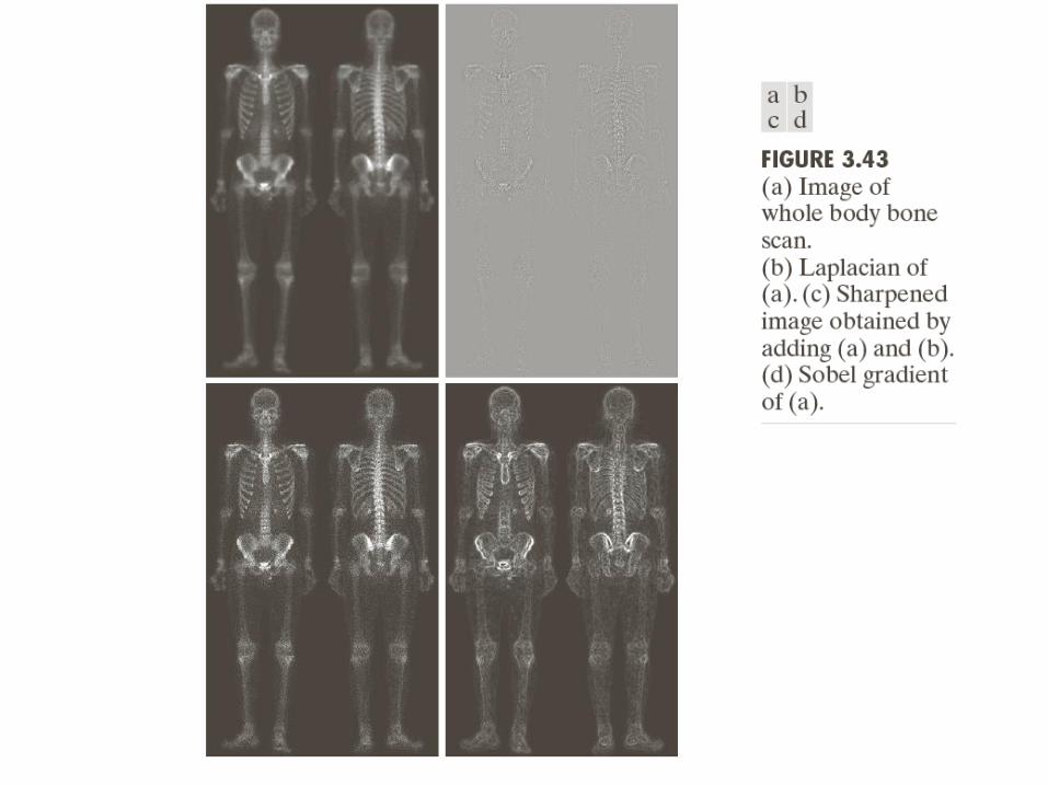
Combining Spatial Enhancement Methods
Successful image enhancement is
typically not achieved using a single
operation
Rather we combine a range of
techniques in order to achieve a final
result
This example will focus on enhancing
the bone scan

Readings from Book (3rd Edn.)
• 3.4 Filtering
• 3.5 Smoothing Filters
• 3.5 Spatial filtering
• Sharpening Filters (Chapter – 3)
• Reading Assignment
• High Boost Filtering (Chap –3.6.3)

68
Acknowledgements
Statistical Pattern Recognition: A Review – A.K Jain et al., PAMI (22) 2000
Pattern Recognition and Analysis Course – A.K. Jain, MSU
Pattern Classification” by Duda et al., John Wiley & Sons.
Digital Image Processing”, Rafael C. Gonzalez & Richard E. Woods, Addison-Wesley, 2002
Machine Vision: Automated Visual Inspection and Robot Vision”, David Vernon, Prentice Hall, 1991
www.eu.aibo.com/
Advances in Human Computer Interaction, Shane Pinder, InTech, Austria, October 2008
Mat
eria
l in
th
ese
slid
es h
as b
een
tak
en f
rom
, th
e fo
llow
ing
reso
urc
es