lecture 7 - 1 ers 482/682 (fall 2002) infiltration ers 482/682 small watershed hydrology
Post on 21-Dec-2015
226 views
TRANSCRIPT
ERS 482/682 (Fall 2002) Lecture 7 - 1
Infiltration
ERS 482/682Small Watershed Hydrology
ERS 482/682 (Fall 2002) Lecture 7 - 2
Definitions
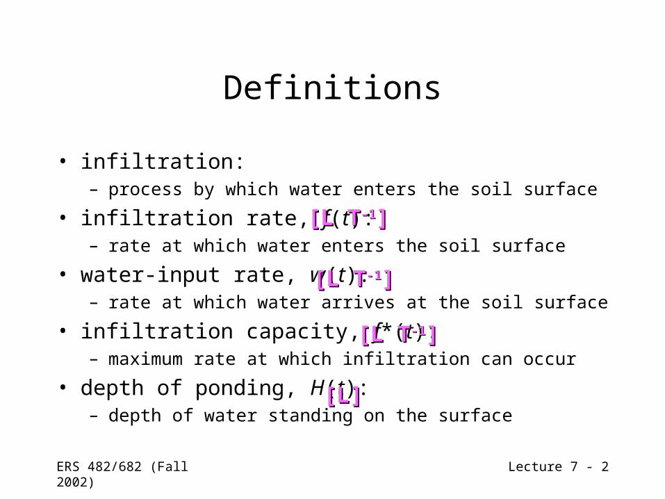
• infiltration:– process by which water enters the soil surface
• infiltration rate, f(t):– rate at which water enters the soil surface
• water-input rate, w(t):– rate at which water arrives at the soil surface
• infiltration capacity, f*(t):– maximum rate at which infiltration can occur
• depth of ponding, H(t):– depth of water standing on the surface
[L T[L T-1-1]]
[L T[L T-1-1]]
[L T[L T-1-1]]
[L][L]
ERS 482/682 (Fall 2002) Lecture 7 - 3
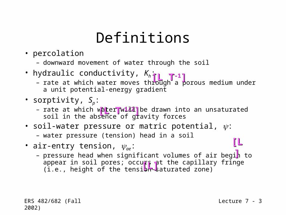
Definitions• percolation
– downward movement of water through the soil
• hydraulic conductivity, Kh:– rate at which water moves through a porous medium under a
unit potential-energy gradient
• sorptivity, Sp:– rate at which water will be drawn into an unsaturated soil in the
absence of gravity forces
• soil-water pressure or matric potential, :– water pressure (tension) head in a soil
• air-entry tension, ae:– pressure head when significant volumes of air begin to appear
in soil pores; occurs at the capillary fringe (i.e., height of the tension-saturated zone)
[L T[L T-1-1]]
[L T[L T-1/2-1/2]]
[L][L]
[L][L]

ERS 482/682 (Fall 2002) Lecture 7 - 4
Why is infiltration important?
ERS 482/682 (Fall 2002) Lecture 7 - 5
Why is infiltration important?
• Determines availability of water for overland flow– Flood prediction
ERS 482/682 (Fall 2002) Lecture 7 - 6
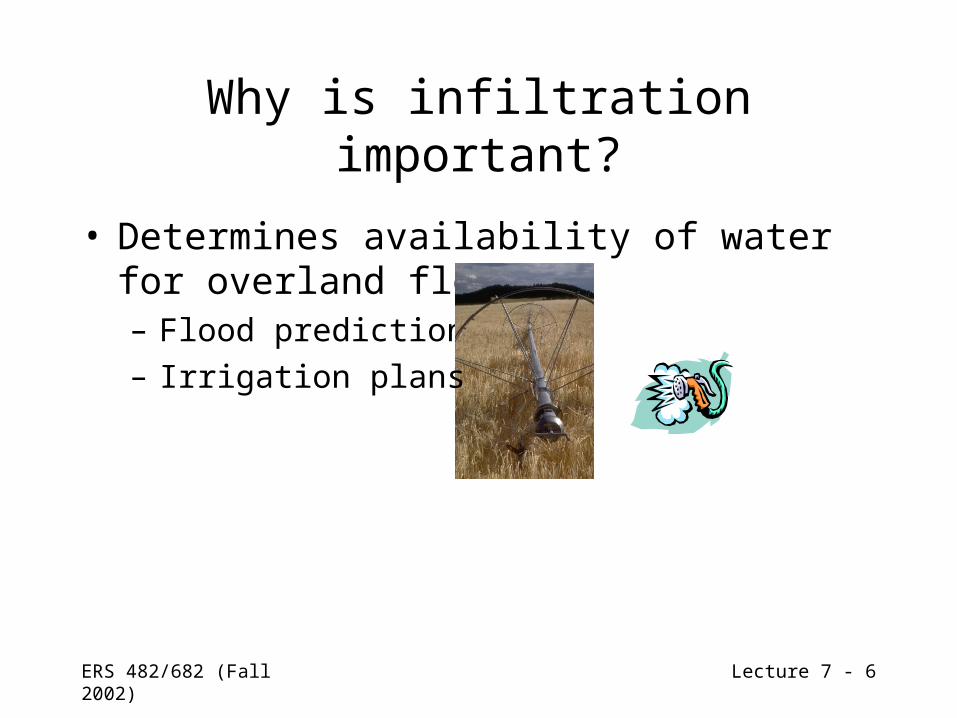
Why is infiltration important?
• Determines availability of water for overland flow– Flood prediction– Irrigation plans

ERS 482/682 (Fall 2002) Lecture 7 - 7
Why is infiltration important?
• Determines availability of water for overland flow– Flood prediction– Irrigation plans– Runoff pollution
• Determines how much water goes into the soil– Groundwater estimates– Water availability for plants
ERS 482/682 (Fall 2002) Lecture 7 - 8
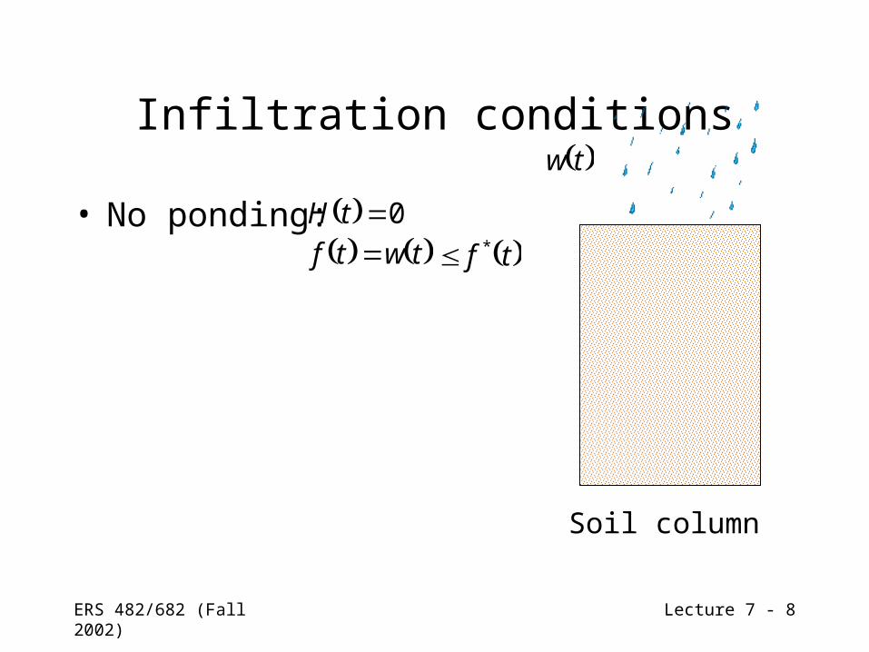
Infiltration conditions
• No ponding:
Soil column
0tH
tw
twtf tf *
ERS 482/682 (Fall 2002) Lecture 7 - 9
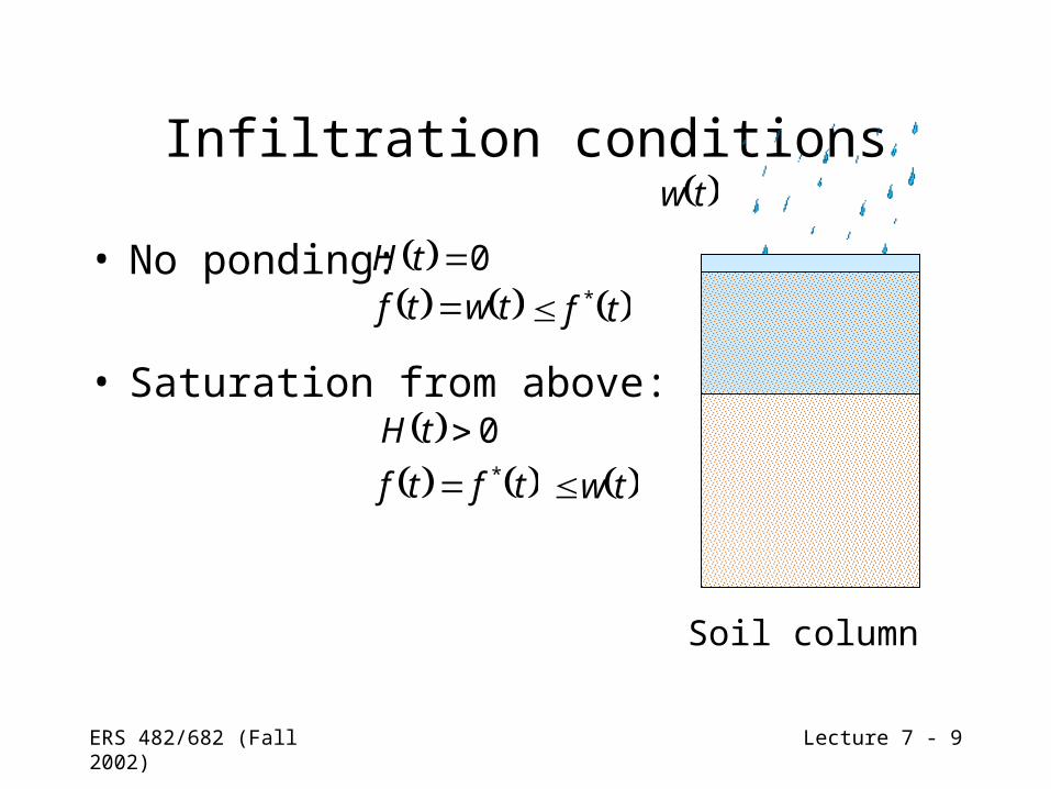
Infiltration conditions
• No ponding:
Soil column
0tH
tw
twtf tf *
• Saturation from above: 0tH
tftf * tw
ERS 482/682 (Fall 2002) Lecture 7 - 10
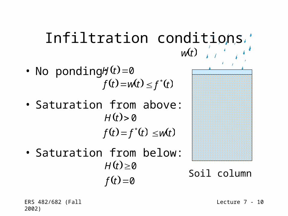
Infiltration conditions
• No ponding:
Soil column
0tH
tw
twtf tf *
• Saturation from above: 0tH
tftf * tw
• Saturation from below: 0tH
0tf

ERS 482/682 (Fall 2002) Lecture 7 - 11
Figure 5.2: Manning (1987)
• Capillarity:– Sorptivity– Matric potential
• Gravity:– Percolation– Hydraulic conductivity

ERS 482/682 (Fall 2002) Lecture 7 - 12
What are models?
Models are representations of the real world
A model is a conceptualizationconceptualization of a system
that retains the essential essential characteristicscharacteristics of
that system for a specific purposespecific purpose.
ERS 482/682 (Fall 2002) Lecture 7 - 13
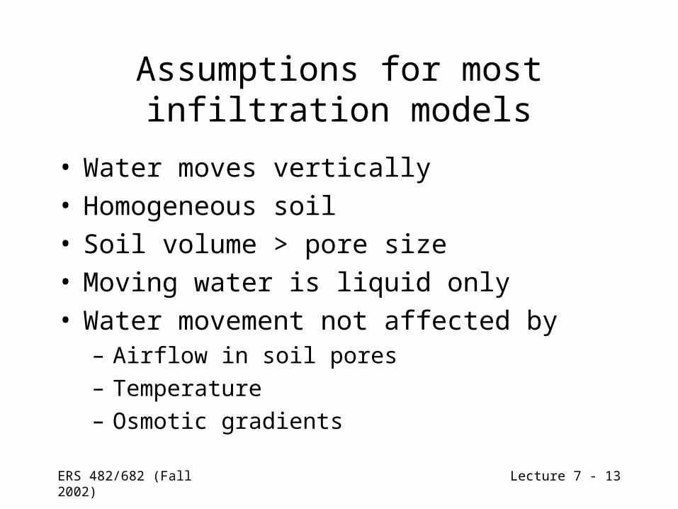
Assumptions for most infiltration models
• Water moves vertically• Homogeneous soil• Soil volume > pore size• Moving water is liquid only• Water movement not affected by
– Airflow in soil pores– Temperature– Osmotic gradients

ERS 482/682 (Fall 2002) Lecture 7 - 14
Infiltration models
• Horton• Kostiakov• Green-Ampt• Philip• Others
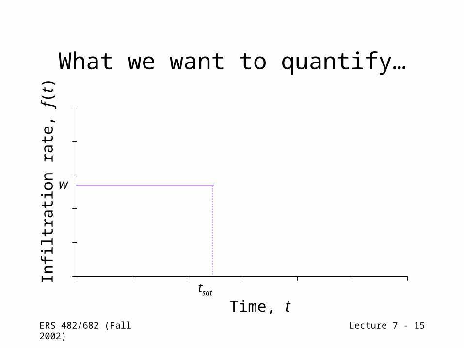
ERS 482/682 (Fall 2002) Lecture 7 - 15
Time, t
Infilt
rati
on r
ate
, f(
t)What we want to quantify…
tsat
w
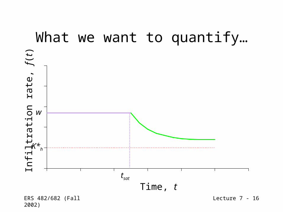
ERS 482/682 (Fall 2002) Lecture 7 - 16
Time, t
Infilt
rati
on r
ate
, f(
t)What we want to quantify…
K*h
tsat
w

ERS 482/682 (Fall 2002) Lecture 7 - 17
Time, t
Infilt
rati
on r
ate
, f(
t)What we want to quantify…
K*h
tsat,1 tsat,2tsat,3
Runoff
f(t)<f*(t) f(t)=f*(t)

ERS 482/682 (Fall 2002) Lecture 7 - 18
What we want to quantify…
Figure 4.2: Brooks et al. (1991)
ERS 482/682 (Fall 2002) Lecture 7 - 19
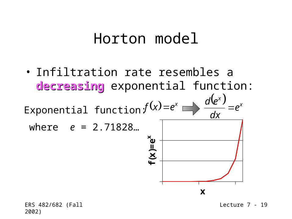
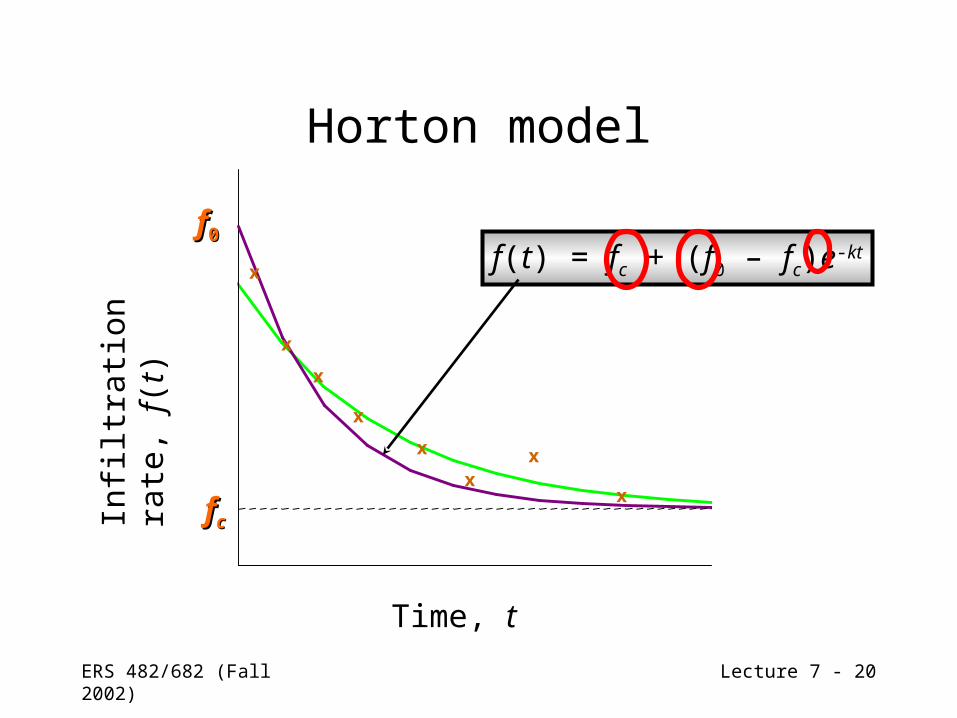
Horton model
• Infiltration rate resembles a decreasingdecreasing exponential function:
Exponential function: xexf
where e = 2.71828…
xx
edx
ed
x
f(x)=
ex
ERS 482/682 (Fall 2002) Lecture 7 - 20
Horton model
Time, t
Infilt
rati
on
rate
, f(
t)
ffcc
ff00
f(t) = fc + (f0 – fc)e-ktx
x
x
x
x
xx
x
ERS 482/682 (Fall 2002) Lecture 7 - 21
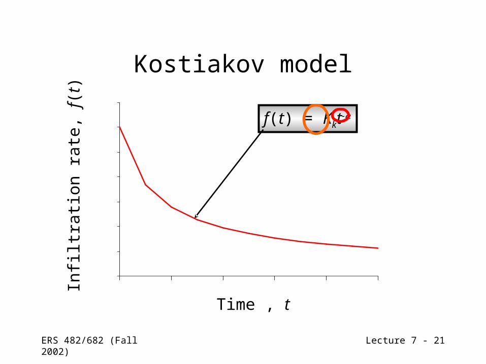
Kostiakov model
Time , t
Infilt
rati
on
rate
, f(
t) f(t) = Kkt-
ERS 482/682 (Fall 2002) Lecture 7 - 22
Water
Soil column
Dry soil = 0
Wet soil =
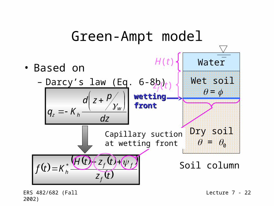
Green-Ampt model
• Based on– Darcy’s law (Eq. 6-8b)
dz
pzdKq w
hz
tz
tztHKtf
f
ffh
*
Capillary suctionat wetting front
wetting wetting frontfront
zf(t)
H(t)
ERS 482/682 (Fall 2002) Lecture 7 - 23
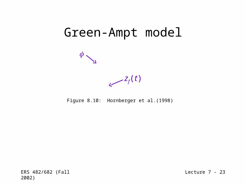
Green-Ampt model
Figure 8.10: Hornberger et al.(1998)
zf(t)
ERS 482/682 (Fall 2002) Lecture 7 - 24
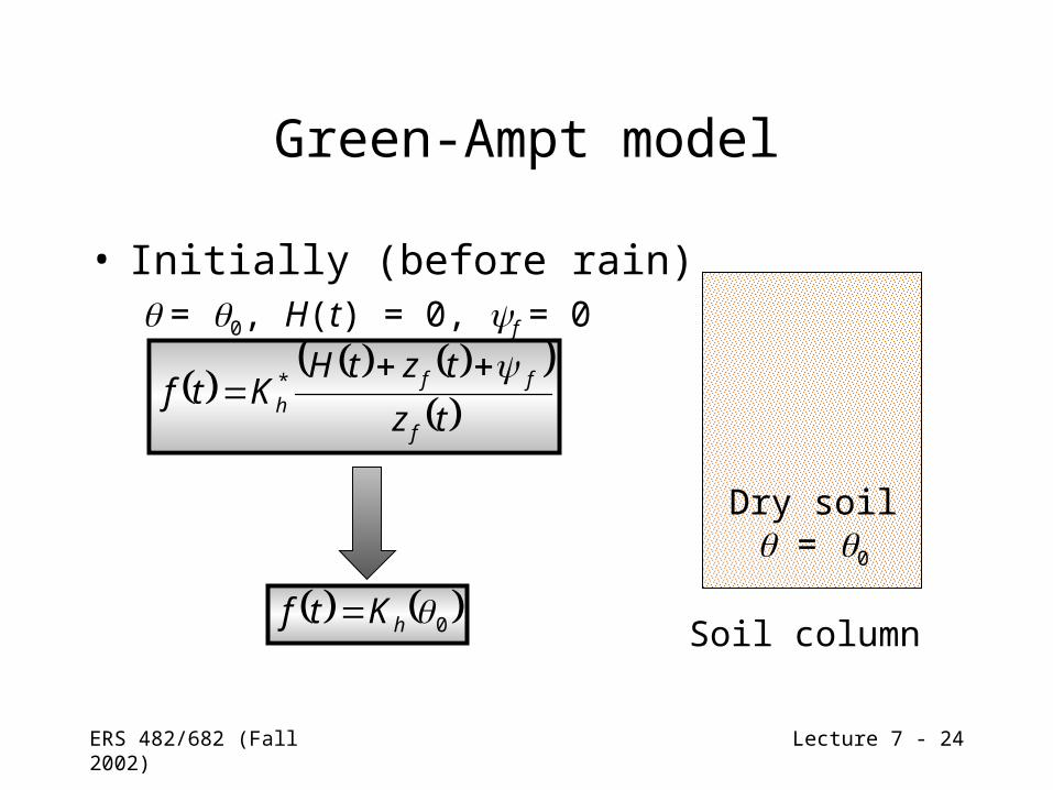
• Initially (before rain) = 0, H(t) = 0, f = 0
Green-Ampt model
Soil column
Dry soil = 0
tz
tztHKtf
f
ffh
*
0hKtf
ERS 482/682 (Fall 2002) Lecture 7 - 25
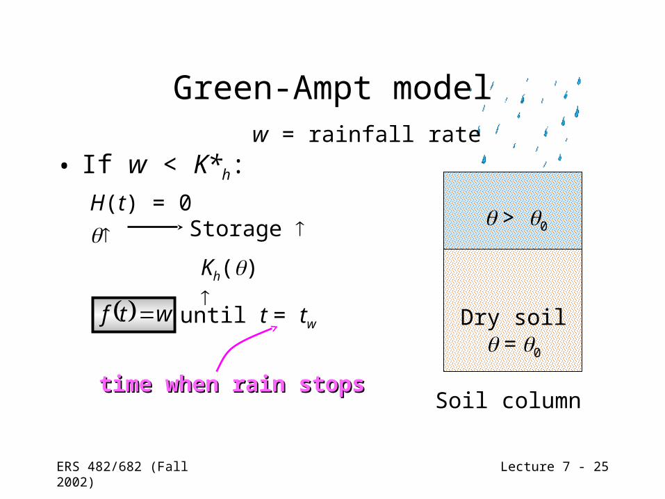
Green-Ampt model
• If w < K*h:H(t) = 0
Soil column
Dry soil = 0
wtf
Kh()
w = rainfall rate
Storage
until t = tw
> 0
time when rain stopstime when rain stops

ERS 482/682 (Fall 2002) Lecture 7 - 26
Green-Ampt model
• If w > K*h:H(t) = 0
Soil column
Dry soil = 0
wtf
Kh() up to up to K*K*hh
Storage
until t=tp
=
time when ponding startstime when ponding starts
ERS 482/682 (Fall 2002) Lecture 7 - 27
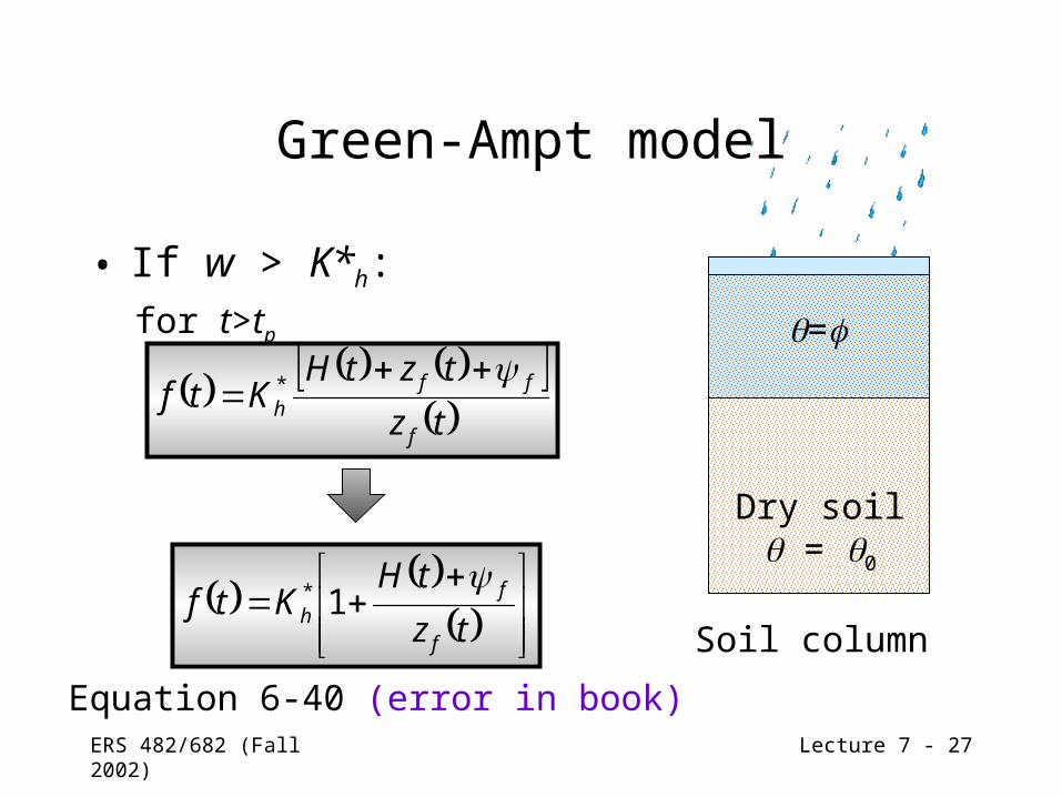
Green-Ampt model
• If w > K*h:
Soil column
Dry soil = 0
for t>tp =
tz
tztHKtf
f
ffh
*
tz
tHKtf
f
fh
1*
Equation 6-40 (error in book)
ERS 482/682 (Fall 2002) Lecture 7 - 28
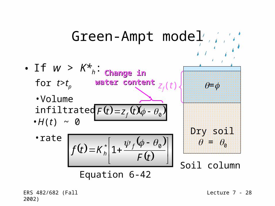
Green-Ampt model
• If w > K*h:
Soil column
Dry soil = 0
for t>tp =
0 tztF f
tFKtf f
h0* 1
Equation 6-42
•Volume infiltrated
zf(t)Change inChange in
water contentwater content
•H(t) ~ 0
•rate

ERS 482/682 (Fall 2002) Lecture 7 - 29
Green-Ampt model
• Difficulties with model– Need to know
• Porosity, • Initial water content, 0
• K*h
f
• See Examples 6-6 and 6-7
measuremeasureTable 6-1Table 6-1
Table 6-1Table 6-1
Equation 6-46 with Table Equation 6-46 with Table 6-16-1
ERS 482/682 (Fall 2002) Lecture 7 - 30
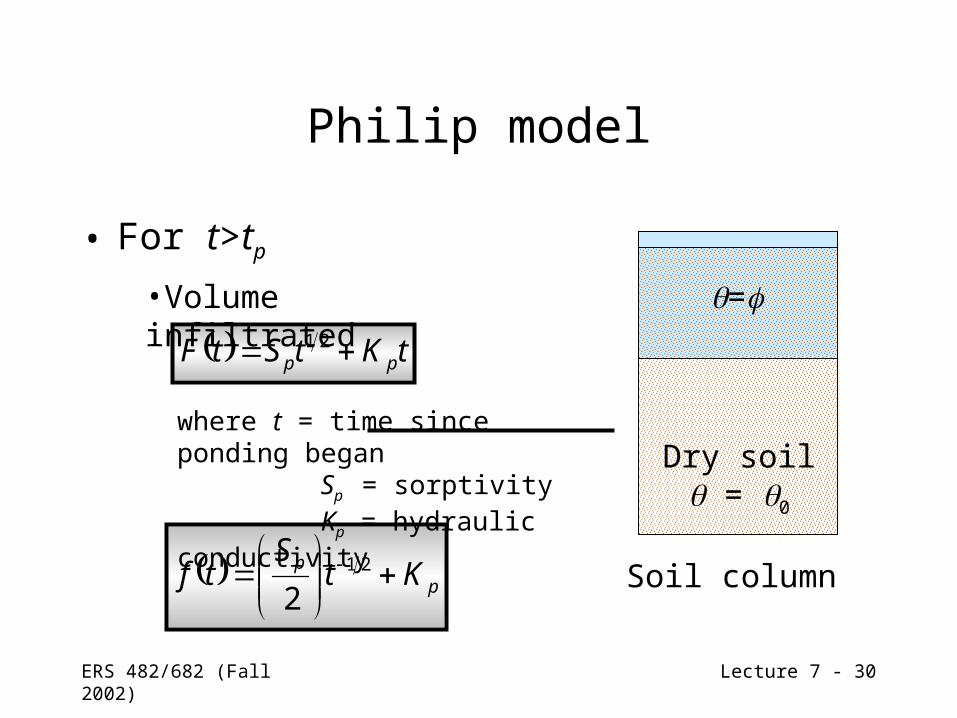
Philip model
• For t>tp
Soil column
Dry soil = 0
=
tKtStF pp 21
•Volume infiltrated
pp Kt
Stf
21
2
where t = time since ponding began Sp = sorptivity Kp = hydraulic conductivity
ERS 482/682 (Fall 2002) Lecture 7 - 31
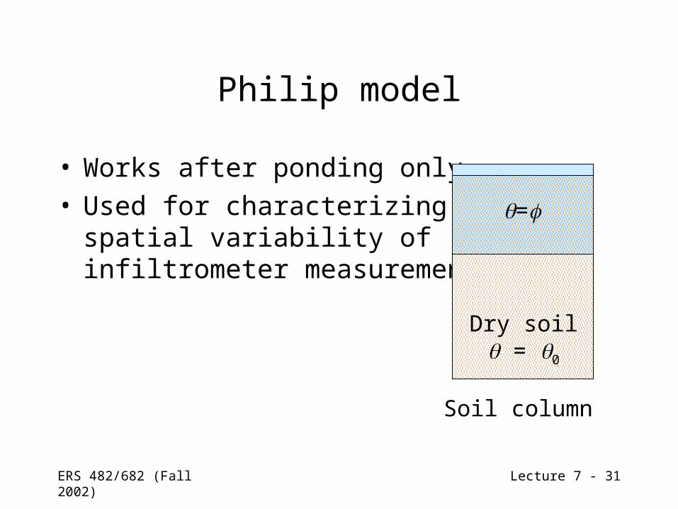
Philip model
• Works after ponding only• Used for characterizing
spatial variability of infiltrometer measurements
Soil column
Dry soil = 0
=
ERS 482/682 (Fall 2002) Lecture 7 - 32
Other models
• Richard’s equation– Physically-based– Numerically intensive
• Morel-Seytoux and Khanji model– Includes viscous resistance
• Smith-Parlange model– Account for different rates of changing
hydraulic conductivity with water content
ERS 482/682 (Fall 2002) Lecture 7 - 33
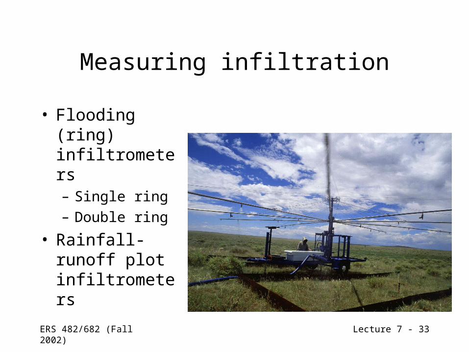
Measuring infiltration
• Flooding (ring) infiltrometers– Single ring– Double ring
• Rainfall-runoff plot infiltrometers
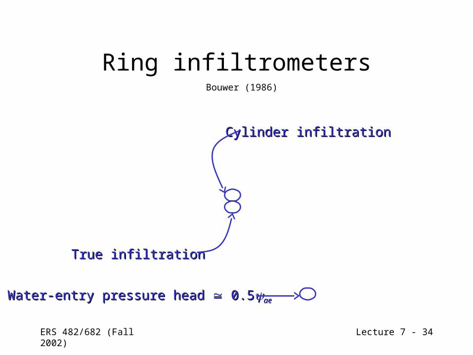
ERS 482/682 (Fall 2002) Lecture 7 - 34
Ring infiltrometersBouwer (1986)
Cylinder infiltrationCylinder infiltration
True infiltrationTrue infiltration
Water-entry pressure head Water-entry pressure head 0.5 0.5aeae
ERS 482/682 (Fall 2002) Lecture 7 - 35
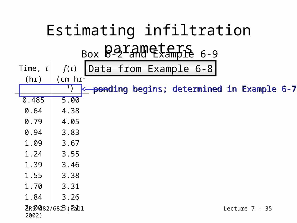
Estimating infiltration parametersBox 6-2 and Example 6-9
Time, t(hr)
f(t)(cm hr-
1)
0.4850.640.790.941.091.241.391.551.701.842.00
5.004.384.053.833.673.553.463.383.313.263.21
ponding begins; determined in Example 6-7ponding begins; determined in Example 6-7
Data from Example 6-8

ERS 482/682 (Fall 2002) Lecture 7 - 36
Estimating infiltration parametersBox 6-2 and Example 6-9
Time, t(hr)
t’(hr)
f(t)(cm hr-
1)
0.4850.640.790.941.091.241.391.551.701.842.00
0.000.1550.3050.4550.6050.7550.9051.0651.2151.3651.515
5.004.384.053.833.673.553.463.383.313.263.21

ERS 482/682 (Fall 2002) Lecture 7 - 37
Estimating infiltration parametersBox 6-2 and Example 6-9
Time, t(hr)
t’(hr)
f(t)(cm hr-
1)
0.4850.640.790.941.091.241.391.551.701.842.00
0.000.1550.3050.4550.6050.7550.9051.0651.2151.3651.515
5.004.384.053.833.673.553.463.383.313.263.21
Least squares approach:Find the parameters that
provide the ‘best fit’ of the model to the observed data
‘best fit’ occurs when sum of the squared differences
between measured and modeled values is
minimized

ERS 482/682 (Fall 2002) Lecture 7 - 38
Estimating infiltration parametersBox 6-2 and Example 6-9
Time, t(hr)
t’(hr)
f(t)(cm hr-
1)
0.4850.640.790.941.091.241.391.551.701.842.00
0.000.1550.3050.4550.6050.7550.9051.0651.2151.3651.515
5.004.384.053.833.673.553.463.383.313.263.21
2
21
2121
11
122
ii
ii
i
i
p
ttN
ttf
ttf
N
S
N
tStf
K ipi
p 2
12 21
Equations 6B2-8 and 6B2-9
note errorin book!
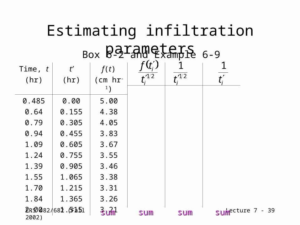
ERS 482/682 (Fall 2002) Lecture 7 - 39
Estimating infiltration parametersBox 6-2 and Example 6-9
Time, t(hr)
t’(hr)
f(t)(cm hr-
1)
0.4850.640.790.941.091.241.391.551.701.842.00
0.000.1550.3050.4550.6050.7550.9051.0651.2151.3651.515
5.004.384.053.833.673.553.463.383.313.263.21
21
i
i
t
tf
21
1
it it1
sumsum sumsum sumsum sumsum

ERS 482/682 (Fall 2002) Lecture 7 - 40
Variability of infiltration
• Factors that affect infiltration rate– Water-input rate or depth of ponding– Hydraulic conductivity at the surface
• Organic surface layers• Frost• Swelling-drying• Inwashing of fine sediment• Anthropogenic modification
ERS 482/682 (Fall 2002) Lecture 7 - 41
Variability of infiltration
• Factors that affect infiltration rate– Water-input rate or depth of ponding– Hydraulic conductivity at the surface
• Organic surface layers• Frost• Swelling-drying• Inwashing of fine sediment• Anthropogenic modification

ERS 482/682 (Fall 2002) Lecture 7 - 42
Variability of infiltration
• Factors that affect infiltration rate– Water content of surface pores– Surface slope and roughness– Chemical characteristics of soil
• hydrophobicity
– Physical/chemical properties of water
Figure 4.5: Brooks et al. (1991)
ERS 482/682 (Fall 2002) Lecture 7 - 43
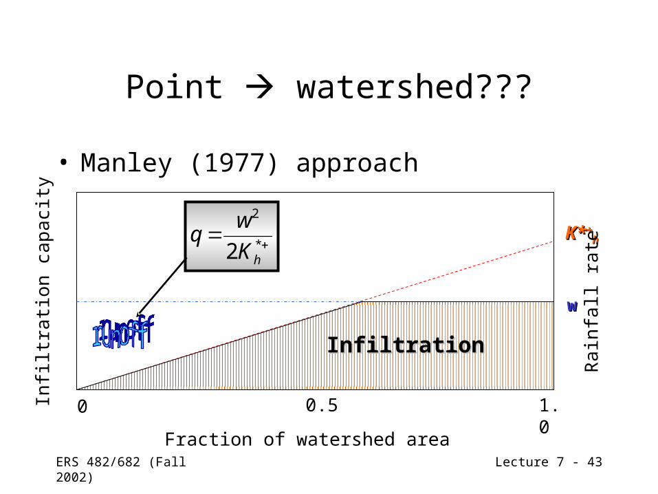
Point watershed???
• Manley (1977) approach
0 1.0
0.5
Fraction of watershed area
Infilt
rati
on
cap
aci
ty
K*K*++hh
ww
Rain
fall
rate
InfiltrationInfiltration
*
2
2 hK
wq
ERS 482/682 (Fall 2002) Lecture 7 - 44
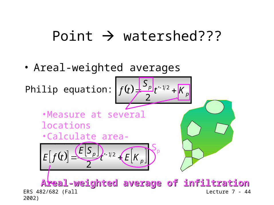
Point watershed???
• Areal-weighted averages
pp Kt
Stf 21
2Philip equation:
•Measure at several locations•Calculate area-weighted average of Sp and Kp
pp KEt
SEtfE 21
2
Areal-weighted average of infiltrationAreal-weighted average of infiltration

ERS 482/682 (Fall 2002) Lecture 7 - 45
Point watershed???
• Divide watershed into subareas– Soil properties– Initial conditions– Etc.
pp KEt
SEtfE 21
2
• Calculate areally-weighted infiltration
ERS 482/682 (Fall 2002) Lecture 7 - 46
Example: Incline Creek Watershed
• Objective: determine which data collection techniques are best for quantifying spatial variations in surface infiltration– Used Philip equation
Sullivan et al. 1996

ERS 482/682 (Fall 2002) Lecture 7 - 47
Watershed size:7.2 km2
ERS 482/682 (Fall 2002) Lecture 7 - 48
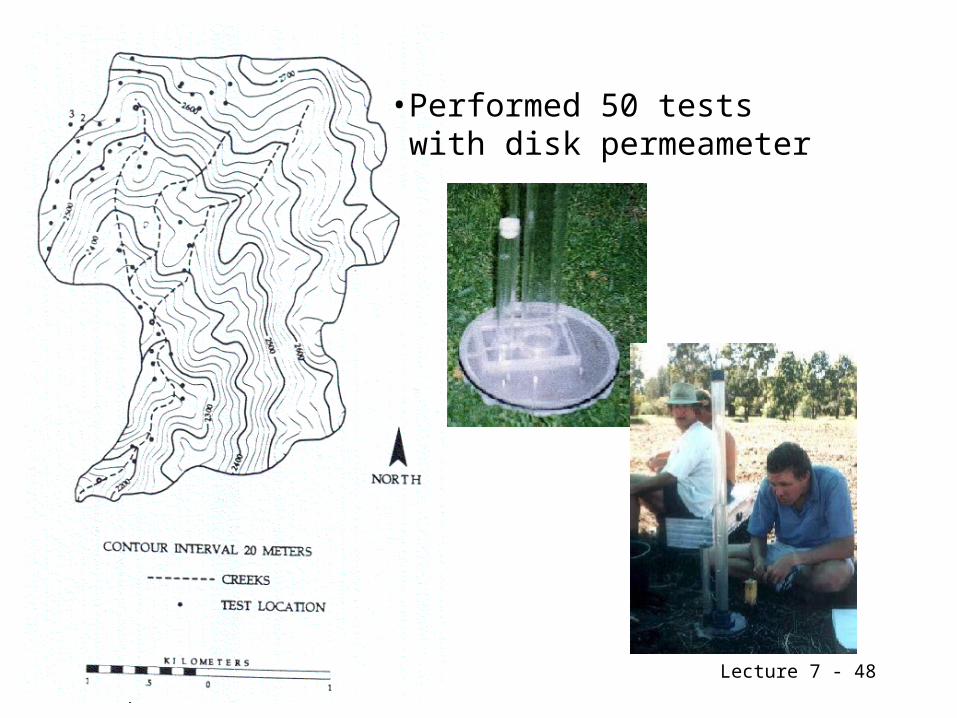
•Performed 50 tests with disk permeameter

ERS 482/682 (Fall 2002) Lecture 7 - 49
•Performed 50 tests with disk permeameter
•Sites were selected based on:AccessibilityMinimal surface disturbanceMacropores were absent
•Tried to pick sites that represented different soil types and vegetative cover

ERS 482/682 (Fall 2002) Lecture 7 - 50
•Created GIS coveragesSoil typesVegetative groupings
•Used field method to determine average areal % of vegetation classification per disk- permeameter test
•Calculated weighted values for Ks based on average areal % vegetation cover
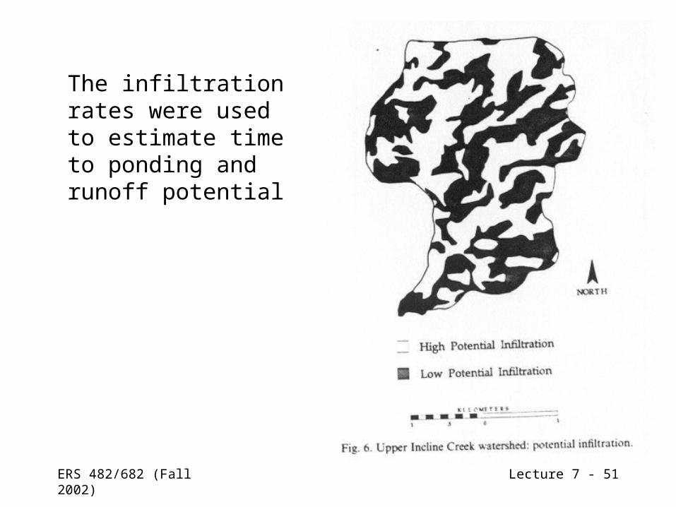
ERS 482/682 (Fall 2002) Lecture 7 - 51
The infiltration rates were used to estimate time to ponding and runoff potential