lecture 9 - university of arizonaatlas.physics.arizona.edu/~shupe/indep_studies...21 7. maxwell...
TRANSCRIPT
1
Lecture 9Lecture 9
Covariant electrodynamicsCovariant electrodynamics
WS2010/11WS2010/11: : ‚‚Introduction to Nuclear and Particle PhysicsIntroduction to Nuclear and Particle Physics‘‘
2
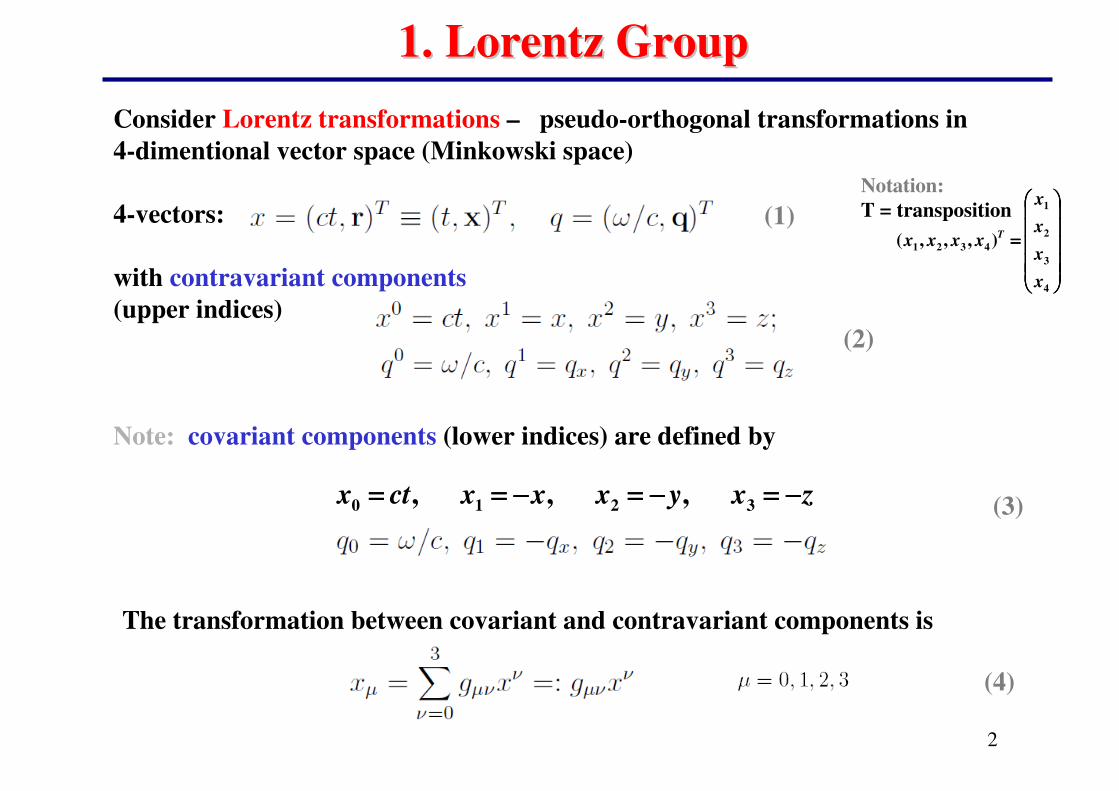
Consider Lorentz transformations – pseudo-orthogonal transformations in
4-dimentional vector space (Minkowski space)
4-vectors:
with contravariant components
(upper indices)
Note: covariant components (lower indices) are defined by
1. Lorentz Group1. Lorentz Group
The transformation between covariant and contravariant components is
zxyxxxctx −−−−====−−−−====−−−−======== 3210 ,,,
(1)
(2)
(3)
(4)
��������������������
����
����
��������������������
����
����
====
4
3
2
1
4321 ),,,(
x
x
x
x
xxxx T
Notation:
T = transposition
3
1. Lorentz Group1. Lorentz Group
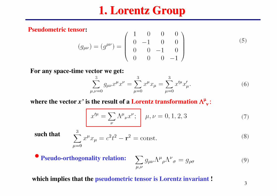
Pseudometric tensor:
(5)
For any space-time vector we get:
where the vector x’ is the result of a Lorentz transformation ΛΛΛΛµµµµν ν ν ν ::::
such that
(6)
(7)
(8)
(9)• Pseudo-orthogonality relation:
which implies that the pseudometric tensor is Lorentz invariant !
4
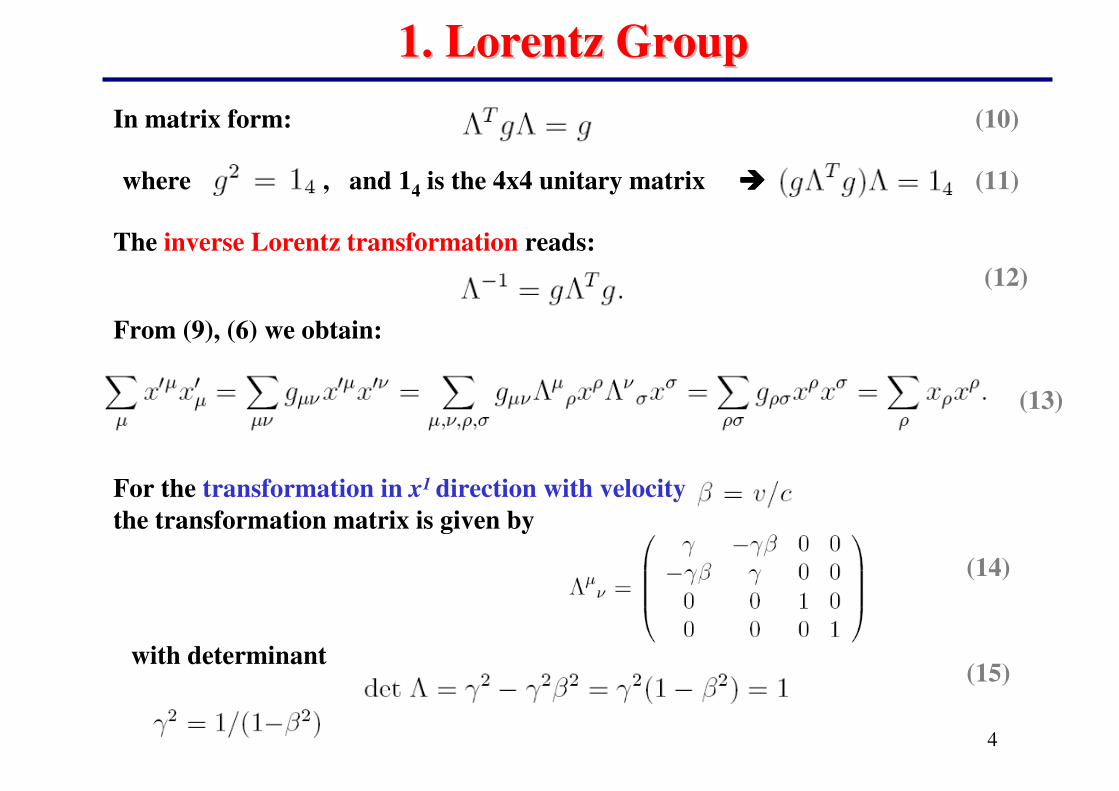
For the transformation in x1 direction with velocity
the transformation matrix is given by
where , and 14 is the 4x4 unitary matrix ����
1. Lorentz Group1. Lorentz Group
In matrix form:
The inverse Lorentz transformation reads:
(10)
(11)
(12)
(13)
(14)
From (9), (6) we obtain:
with determinant(15)
5
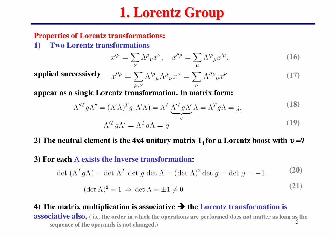
Properties of Lorentz transformations:
1) Two Lorentz transformations
applied successively
appear as a single Lorentz transformation. In matrix form:
2) The neutral element is the 4x4 unitary matrix 14 for a Lorentz boost with υ υ υ υ =0
3) For each ΛΛΛΛ exists the inverse transformation:
4) The matrix multiplication is associative ���� the Lorentz transformation is
associative also, ( i.e. the order in which the operations are performed does not matter as long as the
sequence of the operands is not changed.)
1. Lorentz Group1. Lorentz Group
(16)
(17)
(18)
(19)
(20)
(21)
6
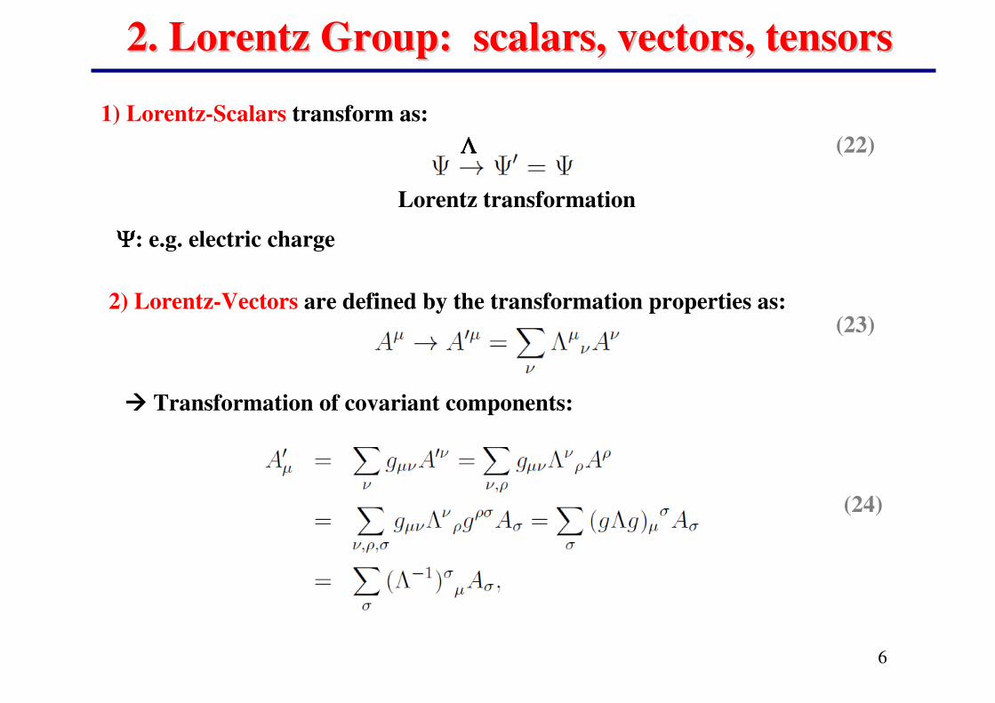
2. Lorentz Group: scalars, vectors, tensors2. Lorentz Group: scalars, vectors, tensors
1) Lorentz-Scalars transform as:
Lorentz transformation
ΛΛΛΛ (22)
ΨΨΨΨ: e.g. electric charge
2) Lorentz-Vectors are defined by the transformation properties as:(23)
(24)
���� Transformation of covariant components:
7
2. Lorentz Group: vectors, tensors2. Lorentz Group: vectors, tensors
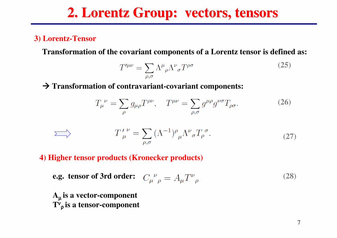
3) Lorentz-Tensor
(25)
(26)
(27)
Transformation of the covariant components of a Lorentz tensor is defined as:
���� Transformation of contravariant-covariant components:
4) Higher tensor products (Kronecker products)
(28)e.g. tensor of 3rd order:
Aµ µ µ µ is a vector-component
Tννννρ ρ ρ ρ is a tensor-component
8
2. Lorentz Group: vectors, tensors2. Lorentz Group: vectors, tensors
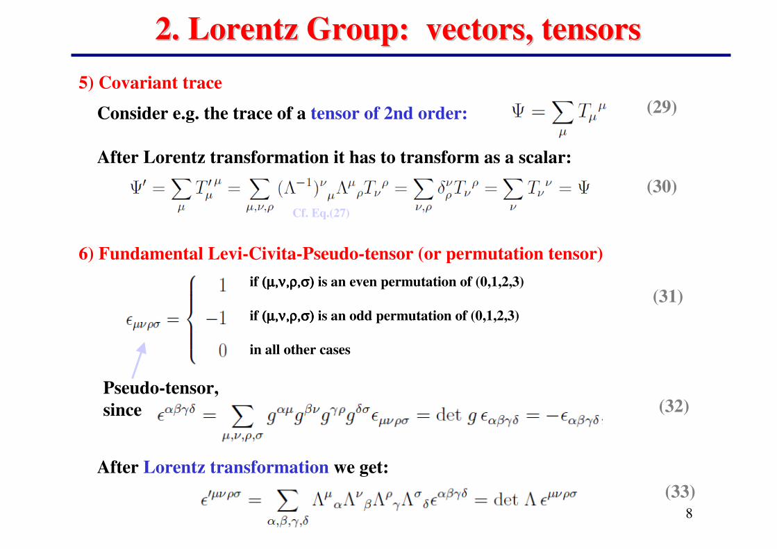
5) Covariant trace
(29)
(30)
(31)
Consider e.g. the trace of a tensor of 2nd order:
After Lorentz transformation it has to transform as a scalar:
6) Fundamental Levi-Civita-Pseudo-tensor (or permutation tensor)
if (µ,ν,ρ,σ)(µ,ν,ρ,σ)(µ,ν,ρ,σ)(µ,ν,ρ,σ) is an even permutation of (0,1,2,3)
if (µ,ν,ρ,σ)(µ,ν,ρ,σ)(µ,ν,ρ,σ)(µ,ν,ρ,σ) is an odd permutation of (0,1,2,3)
in all other cases
(32)Pseudo-tensor,
since
After Lorentz transformation we get:
(33)
Cf. Eq.(27)
9
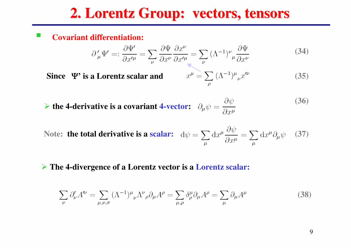
2. Lorentz Group: vectors, tensors2. Lorentz Group: vectors, tensors
� Covariant differentiation:
(34)
(35)
(36)
(37)
ΨΨΨΨ’ is a Lorentz scalar and
� the 4-derivative is a covariant 4-vector:
� The 4-divergence of a Lorentz vector is a Lorentz scalar:
(38)
Since
Note: the total derivative is a scalar:
10
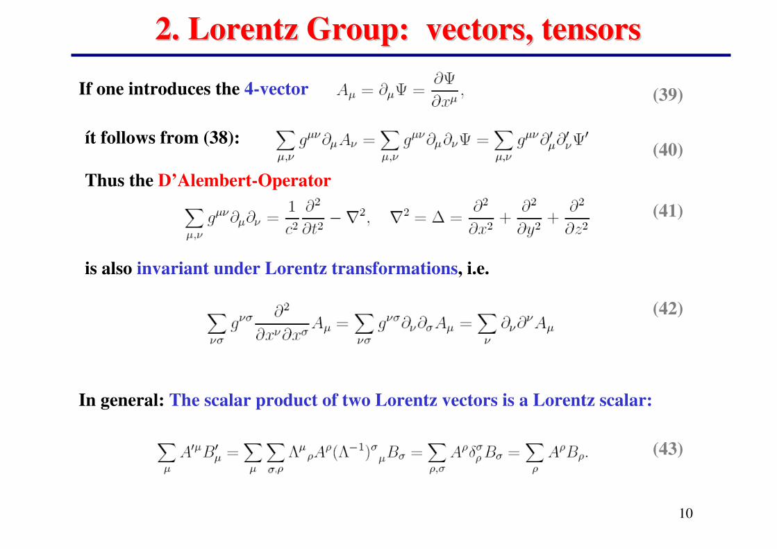
2. Lorentz Group: vectors, tensors2. Lorentz Group: vectors, tensors
If one introduces the 4-vector (39)
(41)
(40)
Thus the D’Alembert-Operator
is also invariant under Lorentz transformations, i.e.
(42)
(43)
In general: The scalar product of two Lorentz vectors is a Lorentz scalar:
ít follows from (38):
11
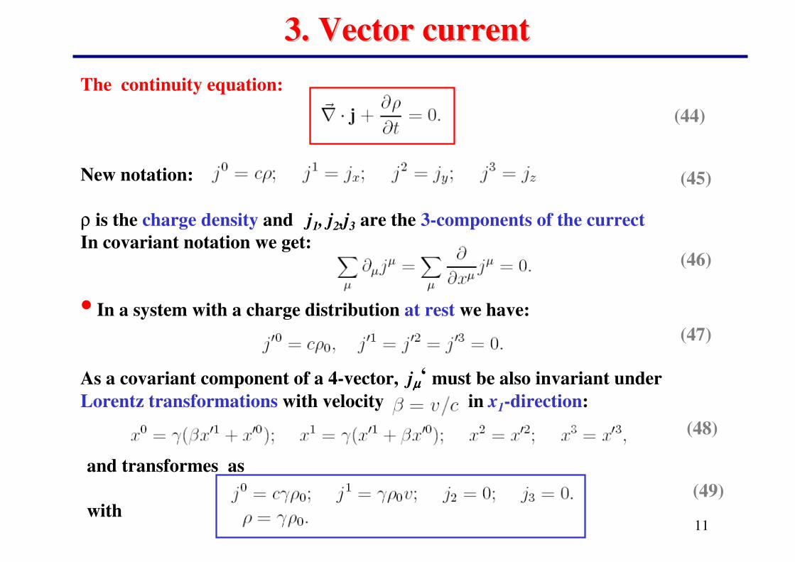
The continuity equation:
New notation:
ρ is the charge density and j1, j2,j3 are the 3-components of the currect
In covariant notation we get:
• In a system with a charge distribution at rest we have:
As a covariant component of a 4-vector, jµµµµ‘ must be also invariant under
Lorentz transformations with velocity in x1-direction:
3. Vector current3. Vector current
(44)
(45)
(46)
(47)
(48)
and transformes as
with(49)
12
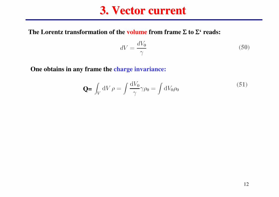
3. Vector current3. Vector current
The Lorentz transformation of the volume from frame ΣΣΣΣ to ΣΣΣΣ‘ reads:
(50)
(51)
One obtains in any frame the charge invariance:
Q=
13
4. The four4. The four--potentialpotential
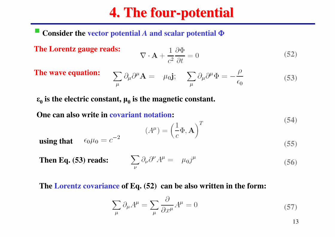
� Consider the vector potential A and scalar potential ΦΦΦΦ
(52)
(53)
The Lorentz gauge reads:
The wave equation:
One can also write in covariant notation:(54)
(55)
(56)
using that
Then Eq. (53) reads:
The Lorentz covariance of Eq. (52) can be also written in the form:
(57)
�0 is the electric constant, �0 is the magnetic constant.
14
4. The four4. The four--potentialpotential
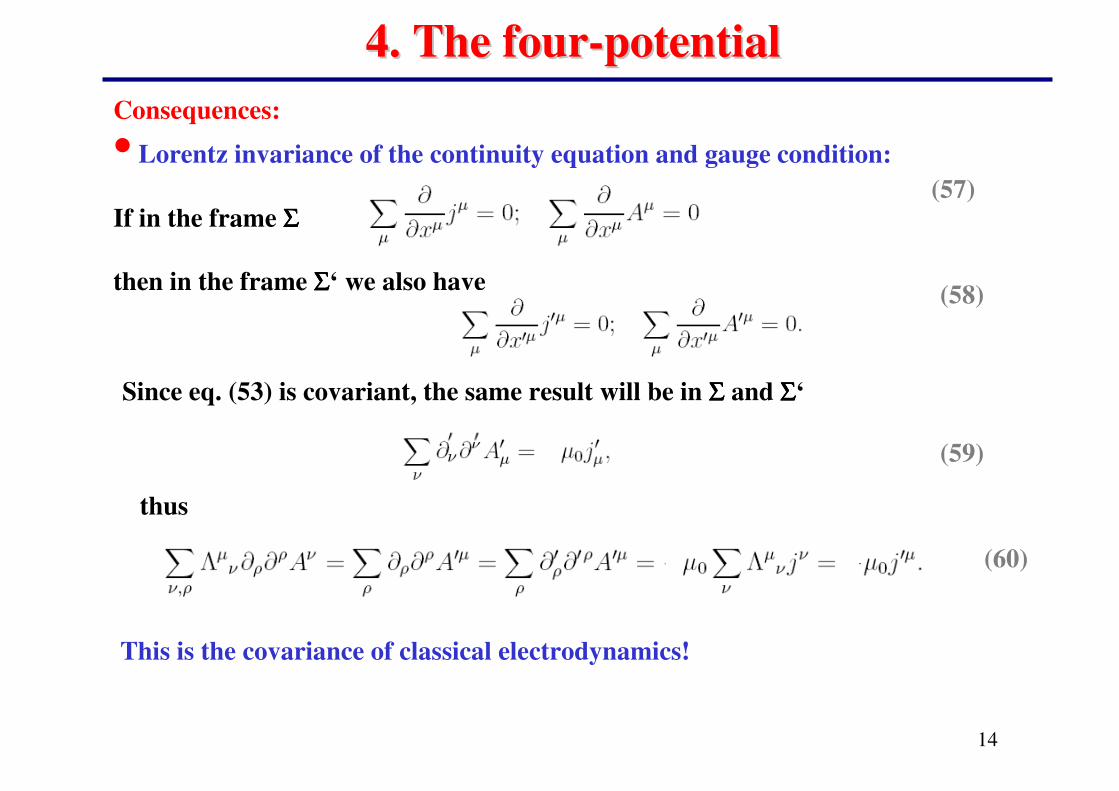
Consequences:
• Lorentz invariance of the continuity equation and gauge condition:
If in the frame ΣΣΣΣ
then in the frame ΣΣΣΣ‘ we also have
(57)
(58)
Since eq. (53) is covariant, the same result will be in Σ Σ Σ Σ and ΣΣΣΣ‘
(59)
(60)
thus
This is the covariance of classical electrodynamics!
15
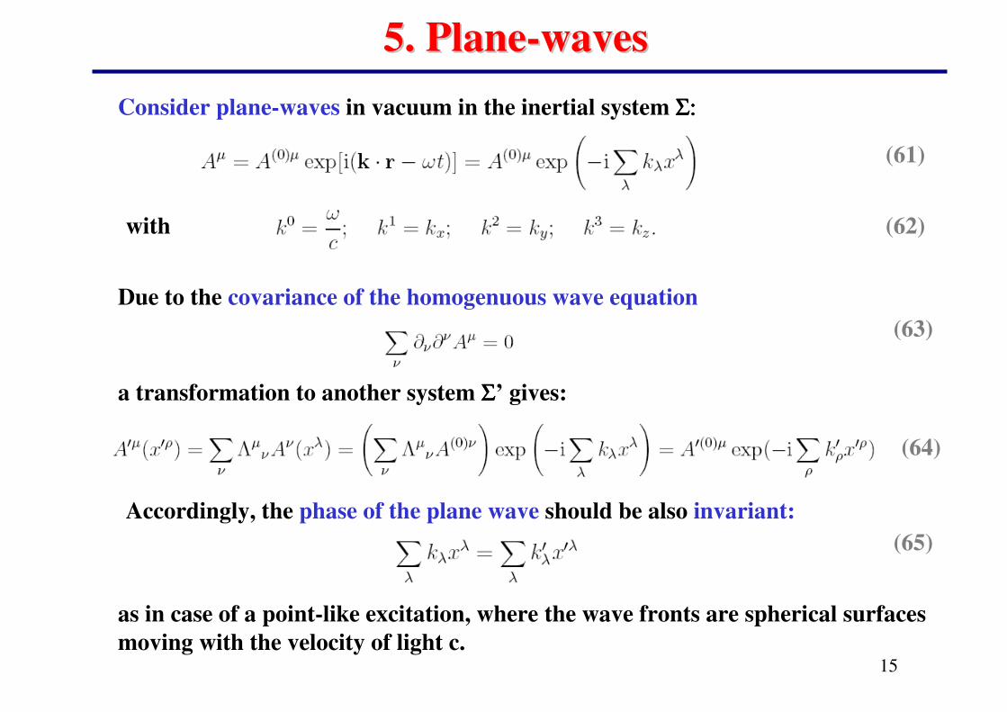
5. Plane5. Plane--waveswaves
(61)
Consider plane-waves in vacuum in the inertial system Σ:Σ:Σ:Σ:
(62)
(63)
Due to the covariance of the homogenuous wave equation
a transformation to another system ΣΣΣΣ’ gives:
(64)
Accordingly, the phase of the plane wave should be also invariant:
as in case of a point-like excitation, where the wave fronts are spherical surfaces
moving with the velocity of light c.
(65)
with
16
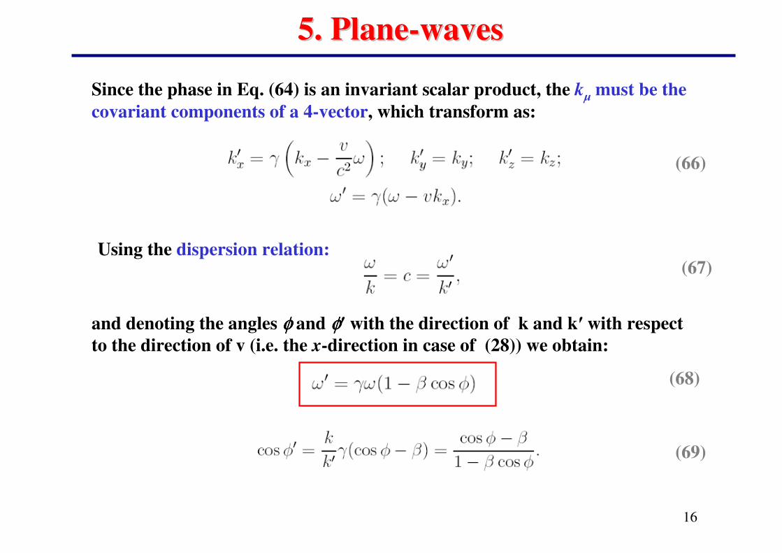
5. Plane5. Plane--waveswaves
(66)
Since the phase in Eq. (64) is an invariant scalar product, the k� must be the
covariant components of a 4-vector, which transform as:
(67)Using the dispersion relation:
(68)
(69)
and denoting the angles φφφφ and φφφφ� with the direction of k and k� with respect
to the direction of v (i.e. the x-direction in case of (28)) we obtain:
17
5. Plane5. Plane--wavewave
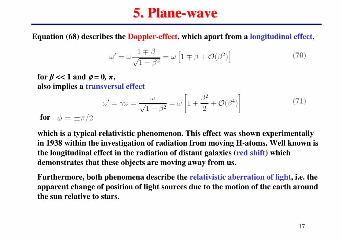
(70)
Equation (68) describes the Doppler-effect, which apart from a longitudinal effect,
(71)
for � << 1 and φφφφ = 0, �,
also implies a transversal effect
for
which is a typical relativistic phenomenon. This effect was shown experimentally
in 1938 within the investigation of radiation from moving H-atoms. Well known is
the longitudinal effect in the radiation of distant galaxies (red shift) which
demonstrates that these objects are moving away from us.
Furthermore, both phenomena describe the relativistic aberration of light, i.e. the
apparent change of position of light sources due to the motion of the earth around
the sun relative to stars.

18
6. Transformation of the fields E and B6. Transformation of the fields E and B
Once knowing the fields A and ΦΦΦΦ, one can compute the fields E and B via
(72)
(73)
(74)
Let‘s rewrite Eq. (72) in covariant form with coordinates x� and the
components of the 4-potential A� . For example we obtain:
Eq. (73) suggests to introduce the antisymmetric field-strength tensor
of second rank
(75)
19
6. Transformation of the fields E and B6. Transformation of the fields E and B
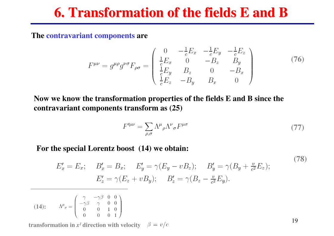
(76)
(77)
The contravariant components are
(78)
Now we know the transformation properties of the fields E and B since the
contravariant components transform as (25)
For the special Lorentz boost (14) we obtain:
transformation in x1 direction with velocity
(14):
20
6. Transformation of the fields E and B6. Transformation of the fields E and B
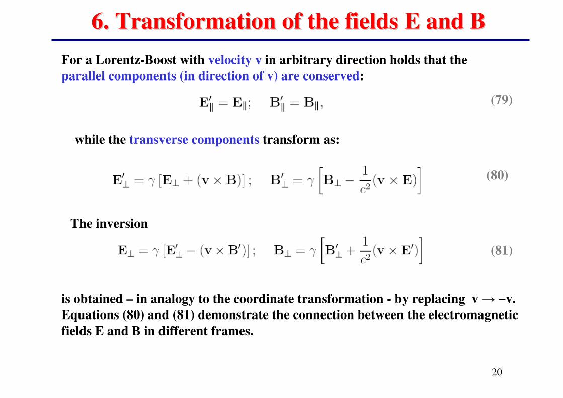
(79)
(80)
(81)
For a Lorentz-Boost with velocity vv in arbitrary direction holds that the
parallel components (in direction of v) are conserved:
while the transverse components transform as:
The inversion
is obtained – in analogy to the coordinate transformation - by replacing v � −v.
Equations (80) and (81) demonstrate the connection between the electromagnetic
fields E and B in different frames.
21
7. 7. Maxwell equationsMaxwell equations
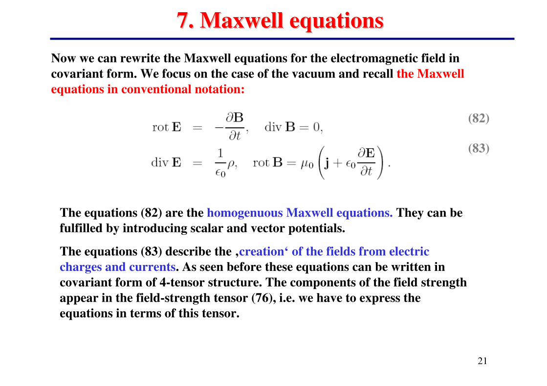
Now we can rewrite the Maxwell equations for the electromagnetic field in
covariant form. We focus on the case of the vacuum and recall the Maxwell
equations in conventional notation:
(82)
(83)
The equations (82) are the homogenuous Maxwell equations. They can be
fulfilled by introducing scalar and vector potentials.
The equations (83) describe the ‚creation‘ of the fields from electric
charges and currents. As seen before these equations can be written in
covariant form of 4-tensor structure. The components of the field strength
appear in the field-strength tensor (76), i.e. we have to express the
equations in terms of this tensor.
22
7. 7. Maxwell equationsMaxwell equations
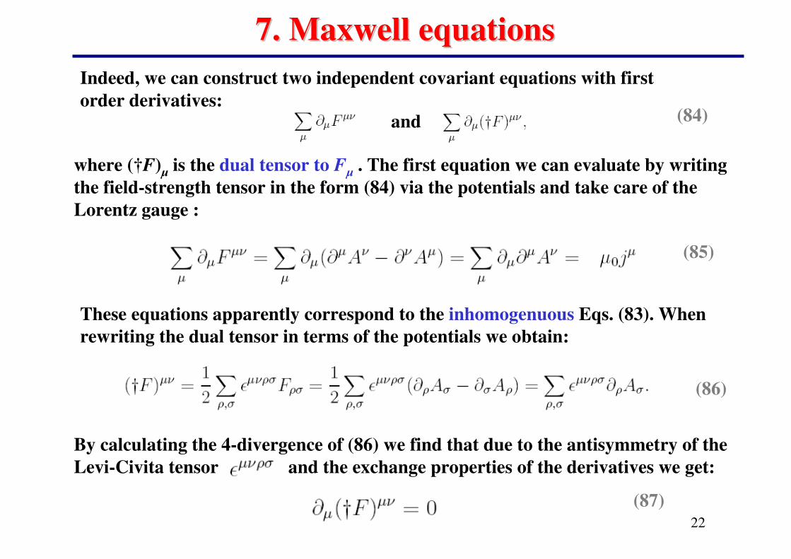
and
where (†F)� is the dual tensor to F� . The first equation we can evaluate by writing
the field-strength tensor in the form (84) via the potentials and take care of the
Lorentz gauge :
(84)
(85)
(86)
These equations apparently correspond to the inhomogenuous Eqs. (83). When
rewriting the dual tensor in terms of the potentials we obtain:
By calculating the 4-divergence of (86) we find that due to the antisymmetry of the
Levi-Civita tensor and the exchange properties of the derivatives we get:
(87)
Indeed, we can construct two independent covariant equations with first
order derivatives:
23
7. 7. Maxwell equationsMaxwell equations
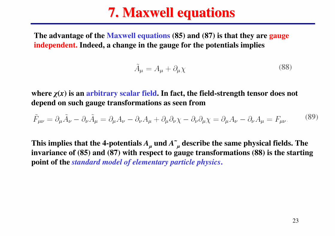
where �(x) is an arbitrary scalar field. In fact, the field-strength tensor does not
depend on such gauge transformations as seen from
The advantage of the Maxwell equations (85) and (87) is that they are gauge
independent. Indeed, a change in the gauge for the potentials implies
This implies that the 4-potentials A� und A˜� describe the same physical fields. The
invariance of (85) and (87) with respect to gauge transformations (88) is the starting
point of the standard model of elementary particle physics.
(88)
(89)
24
8. Coulomb field8. Coulomb field
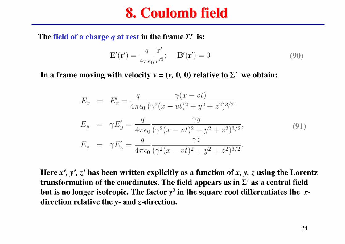
(90)
The field of a charge q at rest in the frame ΣΣΣΣ� is:
(91)
In a frame moving with velocity v = (v, 0, 0) relative to ΣΣΣΣ� we obtain:
Here x�, y�, z� has been written explicitly as a function of x, y, z using the Lorentz
transformation of the coordinates. The field appears as in ΣΣΣΣ� as a central field
but is no longer isotropic. The factor �2 in the square root differentiates the x-
direction relative the y- and z-direction.
25
8. Coulomb Field8. Coulomb Field
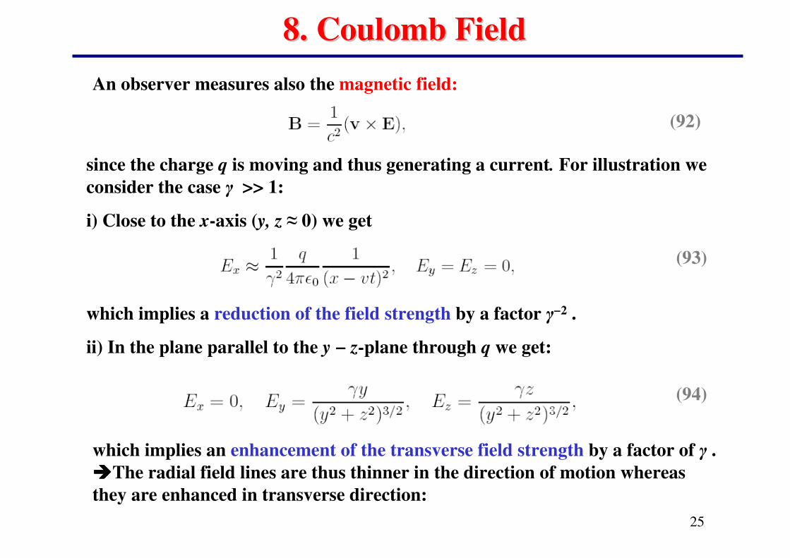
(93)
since the charge q is moving and thus generating a current. For illustration we
consider the case � >> 1:
i) Close to the x-axis (y, z � 0) we get
which implies a reduction of the field strength by a factor �−2 .
ii) In the plane parallel to the y − z-plane through q we get:
(94)
which implies an enhancement of the transverse field strength by a factor of � .
����The radial field lines are thus thinner in the direction of motion whereas
they are enhanced in transverse direction:
An observer measures also the magnetic field:
(92)
26
Covariant electrodynamicsCovariant electrodynamics
Summary:
The basic equations of electrodynamics are covariant
with respect to Lorentz transformations and have the
same form in all inertial systems thus following the
Einstein principle of relativity.