LECTURE :FACTOR ANALYSIS

Rita Osadchy

Based on Lecture Notes by A. Ng

Motivation

Distribution comes from MoG

Have sufficient amount of data: m>>n

Use EM to fit Mixture of Gaussians

If m<<n

difficult to model a single Gaussian

much less a mixture of Gaussian

num. of training points

dimension

Motivation m data points span only a low-dimensional

subspace of

ML estimator of Gaussian parameters:

More generally, unless m exceeds n by some reasonable amount, the maximum likelihood estimates of the mean and covariance may be quite poor.

n

m

i

ixm 1

1 T

i

m

i

i xxm

))((1

1

Singular Can’t compute

Gaussian Density

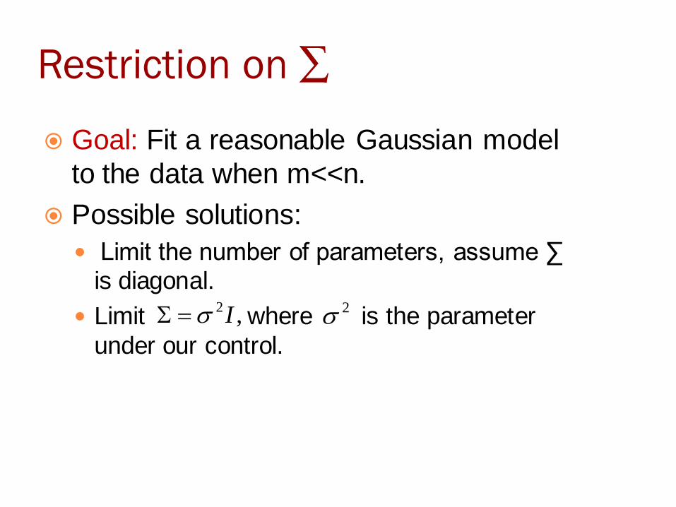
Restriction on ∑

Goal: Fit a reasonable Gaussian model

to the data when m<<n.

Possible solutions:

Limit the number of parameters, assume ∑ is diagonal.

Limit where is the parameter

under our control.

,2I 2

Contours of a Gaussian Density

General ∑ Diagonal ∑

Contours are axis aligned

,2I

Correlation in the data Restricting ∑ to be diagonal means modelling the

different coordinates of the data as being

uncorrelated and independent.

Often, we would like to capture some interesting

correlation structure in the data.

Modeling Correlation

The model we

will see today

Factor Analysis Model

Assume a latent random variable

),( nkz k ),0(~ INz

),(~| zNzx

n knnn is diagonal

The parameters of the model

zx),0(~ N

z

Equivalently,

and are independent.

Example of the generative model

of x 21 , xz

1

2

20

01

0

0

)1,0(~ Nz

)1,0|(zp

1z 2z3z 4z

7z

z2

7 z

zx ),0(~ N2x

1x

Generative process in higher

dimensions

We assume that each data point is

generated by sampling a k-dimension

multivariate Gaussian .

Then, it is mapped to a k-dimensional

affine space of by computing

Lastly, is generated by adding

covariance noise to

iz

n iz

ix

.iz

Definitions

Suppose is r.v., where

Suppose , where

Here …and

Under our assumptions, and are jointly multivariate

Gaussian.

2

1

x

xx

srsr xxx , , 21

),(~ Nx

2221

1211

2

1 ,

, , , , 121121

srrrsr T

2112

1x2x

Partitioned vector

Marginal distribution of x1

By definition of the joint covariance of and

1x 2x

T

T

x

x

x

xExxExCov

22

11

22

11

2221

1211)(

.))(())((

))(())((

22221122

22111111

TT

TT

xxxx

xxxxE

1111111 ][)( T

xxExCov

Marginal distributions of Gaussians are themselves

Gaussian, hence ),(~ 1111 Nx

2

2211 ),()(x

dxxxpxp

Conditional distribution of x1

given x2

Referring to the definition of the multivariate Gaussian

distribution, it can be shown that

where

),,(~| 2|12|121 Nxx

21

1

2212112|1

22

1

221212|1 ),(

x

)(

),()|(

2

2121

xp

xxpxxp

),( N

),( 222 N

Finding the Parameters of FA

model

Assume z and x have a joint Gaussian distribution:

We want to find and

),(~

zxN

z

x

zx

0][ zE ),0(~ INz

.][][][][ EzEzExE

(since )

0

x

zEzx

k

n

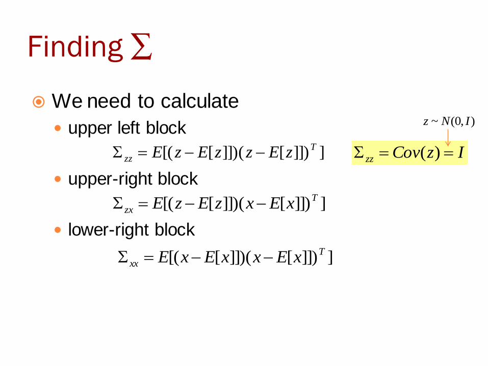
Finding ∑

We need to calculate

upper left block

upper-right block

lower-right block

]]])[]])([[( T

zz zEzzEzE

]]])[]])([[( T

zx xExzEzE

]]])[]])([[( T

xx xExxExE

IzCovzz )(

),0(~ INz

Finding ∑zx

])([]])[])([[( TT zzExExzEzE

=0

][][ TT zEzzE

)(zCov 0][][ EzEindependent

T

Finding ∑xx

Similarly,

]])[])([[( T

xx xExxExE

][ TTTTTT zzzzE

][][ TTT EzzE T

]))([( TzzE

Finding the parameters (cont.)

Putting everything together, we have that,

T

TIN

x

z,

0~

We also see that the marginal distribution of x is given by

),(~ TNx

Thus, given a training set log likelihood of the

parameters is:

m

iix 1}{

m

i

i

TT

iTnxxl

12/ 2

1exp

2

1log),,(

Finding the parameters (cont.)

To perform maximum likelihood estimation, we

would like to maximize this quantity with

respect to the parameters.

But maximizing this formula explicitly is hard,

and we are aware of no algorithm that does

so in closed-form.

So, we will instead use the EM algorithm.

m

i

i

TT

iTnxxl

12/ 2

1exp

2

1log),,(

EM for Factor Analysis

E-step:

M-step:

),|( iiii xzpzQ

i

i z ii

iiii dz

zQ

zxpzQ

i

);,(

logmaxarg

E-step (EM for FA)

We need to compute

Using a conditional distribution of a Gaussian

we find that

),,;|( iiii xzpzQ

)()(0 1

|

i

TT

xz xii

),(~| || iiii xzxzii Nxz

21

1

2212112|1

22

1

221212|1 ),(

x

T

TI

)()(

2

1exp

2

1|

1

||2/1

|

2 iiiiii

ii

xzixz

T

xzi

xz

kii zzzQ

1

| )( TT

xz Iii

1 12

1

22

)( 22 x

11 121

22

12

M-step (EM for FA)

Maximize:

with respect to the parameters

We will work out the optimization with respect to

Derivations of the updates for is an exercise

(Do it!)

i

ii

iim

i z

ii dzzQ

zxpzQ

i

),,;,(log

1

,,

,

Update for Λ

i

ii

iim

i z

ii dzzQ

zxpzQ

i

),,;,(log

1

iiiiii

m

i z

ii dzzQzpzxpzQ

i

]log)(log),,;|([log1

]log)(log),,;|([log1

~ iiiii

m

i

Qz zQzpzxpEii

Expectation with respect to , drawn from iz iQ

Update for Λ (cont.)

]log)(log),,;|([log1

~ iiiii

m

i

Qz zQzpzxpEii

Remember that We want to maximize this expression

with respect to Λ

)],,;|([log1

~

ii

m

i

Qz zxpEii

)()(2

1exp

2

1log 1

2/12/1

ii

T

iin

m

i

zxzxE

)()(2

12log

2log

2

1 1

1

ii

T

ii

m

i

zxzxn

E

Do not depend on Λ

),(~| zNzx

Update for Λ (cont.)

)()(2

1 1

1

ii

T

ii

m

i

zxzxE

Take derivative with respect to Λ

; ,tr aaa

scalar

)()(2

1tr 1

1

ii

T

ii

m

i

zxzxE

)(tr 2

1tr 11

1

i

TT

ii

TT

i

m

i

xzzzE

Simplify:

)(tr 2

1tr 11

1

i

TT

ii

TT

i

m

i

xzzzE

trtr BAAB

Update for Λ (cont.)

CABCABCABA TTTTTT

AT tr

T

ii

TT

ii

Tm

i

zxzzE )(tr 2

1tr 11

1

T

ii

T

ii

m

i

zxzzE )(11

1

Update for Λ (cont.)

Setting this to zero and simplifying, we get:

T

ii

T

ii

m

i

zxzzE )(11

1

T

iQz

m

i

i

T

ii

m

i

Qz zExzzEiiii ~

11

~

Solving for Λ, we obtain:

1

1

~~

1

T

ii

m

i

Qz

T

iQz

m

i

i zzEzExiiii

Since is Gaussian with mean and covariance | ii xzii xz | Q

T

xz

T

iQz iiiizE |~ ][

iiiiiiii xz

T

xzxz

T

iiQz zzE |||~ ][

][][][)( TT YEYEYYEYCov

)(][][][ YCovYEYEYYE TT

hence,

Update for Λ (cont.)

1

1

~~

1

T

ii

m

i

Qz

T

iQz

m

i

i zzEzExiiii

T

xz

T

iQz iiiizE |~ ][

iiiiiiii xz

T

xzxz

T

iiQz zzE |||~ ][

1

1

||||

1

m

i

xz

T

xzxz

T

xz

m

i

i iiiiiiiix

substitute

M-step updates for μ and Ψ

),,;|( iiii xzpzQ

m

i

ixm 1

1

Doesn’t depend on ,

hence can be computed once for all the

iterations .

T

xz

T

xzxz

T

ixz

TT

xzi

T

i

m

i

i iiiiiiiiiixxxx

m

)(1

|||||

1

The diagonal

(contains only diagonal entrees)

iiii

Probabilistic PCA

Probabilistic, generative view of data

MDx z ,

Compare

Probabilistic PCA

FA

diagonal, axis-aligned

spherical

Probabilistic PCA

The columns of W are the principle

components.

Can be found using

ML in closed form

EM ( more efficient when only few eigenvectors are required, avoids evaluation

of data covariance matrix)

Other advantages (see Bishop, Ch.12.2)