lecture notes 7 - high energy physics at the...

UIUC Physics 436 EM Fields & Sources II Fall Semester, 2015 Lect. Notes 7.5 Prof. Steven Errede

© Professor Steven Errede, Department of Physics, University of Illinois at Urbana-Champaign, Illinois 2005-2015. All Rights Reserved.

1

LECTURE NOTES 7.5

Dispersion: The Frequency-Dependence of the Electric Permittivity

and the Electric Susceptibility 1e o

Over the entire EM frequency interval 0 ,f Hz the speed of propagation propv of

monochromatic (i.e. single-frequency) EM waves in matter is often not constant, not independent of frequency: propv constant; frequency, propfcn f v f , because matter - at the

microscopic scale - is composite - comprised of atoms/molecules – which have resonances in energy/energy levels – which are governed by the laws of quantum mechanics…

The frequency-dependence of the wavelength , or wavenumber 2k ,

and linear momentum p associated with macroscopic EM waves propagating in a dispersive

medium arises from the frequency-dependence of the macroscopic electric permittivity

(or equivalently the electric susceptibility e since:

1o e .

The frequency-dependence of the macroscopic electric permittivity is known as

dispersion; a medium that has fcn is known as a dispersive medium.

For non-magnetic/non-conducting linear/homogeneous/isotropic media, the index of refraction

on . Thus, if: 1o e then: on .

For a wave packet (= a group {= superposition/linear combination} of waves of many frequencies – as explained by Mssr. Fourier), the envelope of the wave packet travels with (in general, frequency-dependent) group speed = speed at which energy in the wave flows:

1" " 1

g

dkdv

dk dk d d

A propagating wave packet: f kz t

v

k

1

g

dkv

d

A space-point z t on the waveform moves - with constant phase kz t

with (in general, frequency-dependent) phase speed v k .

Hence: ,z t k v t . Note that {in general}: gv v .



2

If v k is frequency-dependent, and 1

gv dk d v

{e.g. as in

the case for surface waves on water, where 2 gv v } the relationship between and gv v

depends on the detailed physics of the medium (as we shall soon see. . . ). Note that in certain circumstances, v can exceed c {= speed of light in the vacuum} but in these situations, no

energy (and/or information) is transmitted at super-luminal speeds – energy/information is transmitted at gv < c always, by causality…

A physical/mechanical example: calculate the phase speed of the intersection point of the two halves of a scissors as the blades of the scissors are closed. {Answer: scissorsv !!!}

Dispersion Phenomena in Linear Dielectrics

In a non-conducting, linear, homogeneous, isotropic medium there are no free electrons (i.e. 0free r

). Atomic electrons are permanently bound to nuclei of atoms comprising the

medium. no preferential direction / no preferential directions in such an {isotropic} medium.

Suppose each atomic electron (charge –e) in a dielectric is displaced by a small distance r

from its equilibrium position, e.g. by application of a static electric field ˆE r r direction.

The resulting macroscopic electric polarization (aka electric dipole moment per unit volume) is:

ber n p r

where: b

en = bound atomic electron number density 3#e m

and the {induced} atomic/molecular electric dipole moment is: p r er

{here}, where r

is the

{vector} displacement of the atomic electron from its equilibrium { r

= 0} position.

Thus: b be er n p r n er

The atomic electrons are each elastically bound to their equilibrium positions with a force

constant ek N m . The force equation for each atomic electron is thus: e eF r eE r k r

.

Hence: er eE r k

.

The static polarization is therefore given by: 2b

b b b ee e e

e e

eE r n er n p r n er n e E r

k k

However, if the E

-field e.g. varies harmonically with time, i.e. ˆ, ; i kz toE E r t E e n

due to a monochromatic EM plane wave incident on an atom, the above relation is incorrect !

A more correct {but “semi-classical”} approach to treat this situation is to consider the bound atomic electrons as classical, damped, forced harmonic oscillators (driven by the incident electric field), as mathematically described by the following differential equation:

; ; ; , ;e e em r t m r t k r t eE r t ← inhomogeneous 2nd-order differential eqn.

The damping constant rads sec represents the effect of EM re-radiation by the atom {here}.



3

2

2

; ;; , ;

e

e e e

m a

r t r tm m k r t eE r t

t t

31electron mass 9.1 10em kg

Suppose the driving/forcing term varies sinusoidally/is harmonic/periodic with angular

frequency , i.e. ˆ, ; , ; i te oF r t eE r t eE e r because ˆ, ; i t

oE r t E e r .

n.b. The electric field E

is complex E and plane-polarized in the r̂ -direction.

The inhomogeneous force equation becomes: î te e e om r m r k r eE e r with complex

time-domain vector displacement amplitude: ˆ; ;r t r t r . In the steady state, we have:

î te e e om r m r k r eE e r

Since ;r t physically represents the complex vector spatial displacement of an atomic

electron from its equilibrium { 0r

} position, then: ˆ ˆ; ; i tor t r t r r e r

Thus: î te e e om r m r k r eE e r

2

2

; ;; , ;e e e

r t r tm m k r t eE r t

t t

2 i te om r e i t

e oi m r e i te ok r e i t

oeE e

2e e e o om k i m r eE characteristic equation

Divide this equation through by em : 2 eo o

e e

k ei r E

m m

Define: 20

e

e

k

m

or: 0e

e

k

m = characteristic/natural resonance {angular} frequency. Then:

2 20 o o

e

ei r E

m

or:

2 20

1o o

e

er E

m i

Note that the complexness of frequency-domain or is in the denominator.

We can move it to the numerator using the following standard “trick”/procedure:

If: 2 2

1 1 x iy x iyz

x iy x iy x iy x y

where: 2 2

xe z

x y

and: 2 2

ym z

x y

n.b. we have neglected the

ev B eE term here...

Velocity-dependent damping term

damping constant

Potential Force (binding of atomic electrons to atom)

Driving Force

Bound atomic electron complex frequency-

domain spatial displacement amplitude



4

Thus:

2 20

2 2 2 2 2 20 0 0

2 20

2 2 2 20 0

2 20

22 2 2 20 0

*

*

e e

e

e

e eo om m

o

eom

eom

iE Er

i i i

iE

i i

E i

i

2 20i

2 2

2 20

22 2 2 20

e

eom

iE

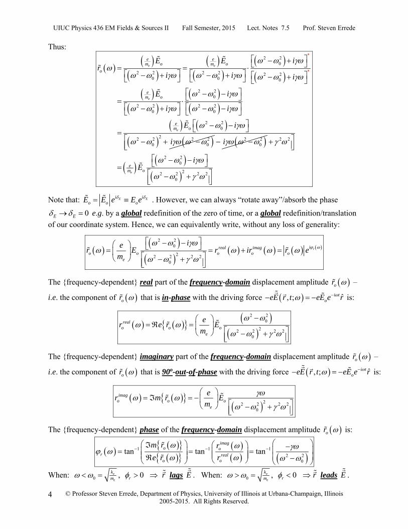
Note that: E Ei io o oE E e E e . However, we can always “rotate away”/absorb the phase

0E E e.g. by a global redefinition of the zero of time, or a global redefinition/translation

of our coordinate system. Hence, we can equivalently write, without any loss of generality:

2 2

0

22 2 2 20

rireal imago o o o o

e

ier E r ir r e

m

The {frequency-dependent} real part of the frequency-domain displacement amplitude or –

i.e. the component of or that is in-phase with the driving force ˆ, ; i toeE r t eE e r

is:

2 20

22 2 2 20

realo o o

e

er e r E

m

The {frequency-dependent} imaginary part of the frequency-domain displacement amplitude or –

i.e. the component of or that is 90o-out-of-phase with the driving force ˆ, ; i toeE r t eE e r

is:

22 2 2 2

0

imago o o

e

er m r E

m

The {frequency-dependent} phase of the frequency-domain displacement amplitude or is:

1 1 1

2 20

tan tan tanimag

o or real

oo

m r r

re r

When: 0e

e

km , 0r r

lags E . When: 0

e

e

km , 0r r

leads E .



5

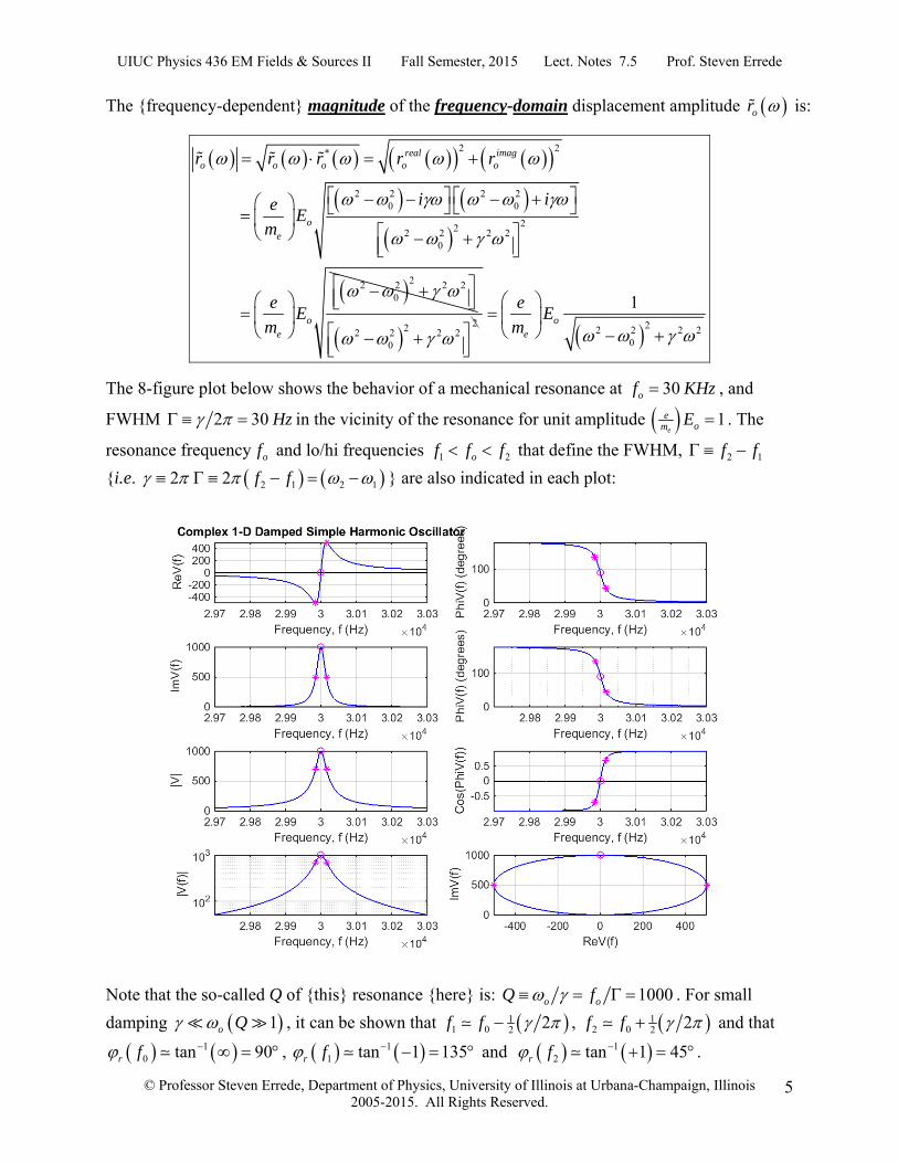
The {frequency-dependent} magnitude of the frequency-domain displacement amplitude or is:

2 2*

2 2 2 20 0

222 2 2 20

22 2 2 20

real imago o o o o

oe

oe

r r r r r

i ieE

m

eE

m

222 2 2 2

0 22 2 2 2

0

1o

e

eE

m

The 8-figure plot below shows the behavior of a mechanical resonance at 30 of KHz , and

FWHM 2 30 Hz in the vicinity of the resonance for unit amplitude 1e

eom E . The

resonance frequency of and lo/hi frequencies 1 2of f f that define the FWHM, 2 1f f

{i.e. 2 1 2 12 2 f f } are also indicated in each plot:

Note that the so-called Q of {this} resonance {here} is: 1000o oQ f . For small

damping 1o Q , it can be shown that 11 0 2 2f f , 1

2 0 2 2f f and that

10 tan 90r f , 1

1 tan 1 135r f and 12 tan 1 45r f .



6

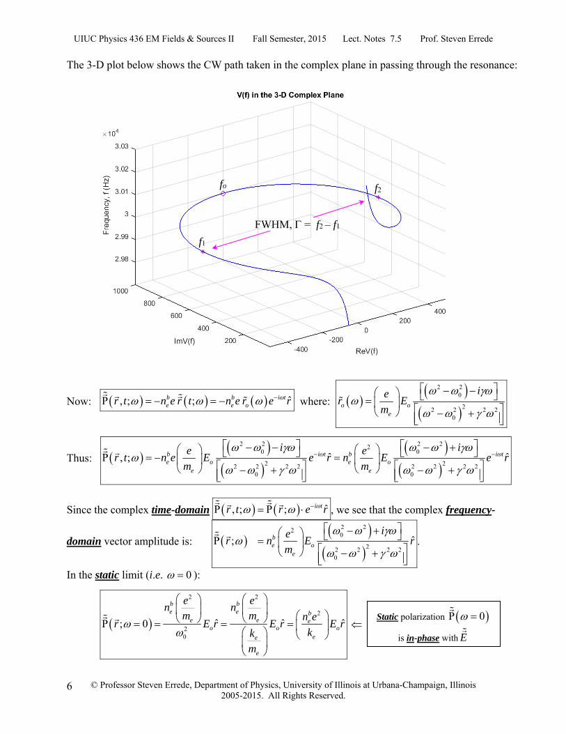
The 3-D plot below shows the CW path taken in the complex plane in passing through the resonance:

Now: ˆ, ; ; b b i te e or t n e r t n e r e r

where:

2 20

22 2 2 20

o oe

ier E

m

Thus:

2 2 2 220 0

2 22 2 2 2 2 2 2 20 0

ˆ ˆ, ; b i t b i te o e o

e e

i ie er t n e E e r n E e r

m m

Since the complex time-domain ˆ, ; ; i tr t r e r , we see that the complex frequency-

domain vector amplitude is:

2 220

22 2 2 20

ˆ; be o

e

ier n E r

m

.

In the static limit (i.e. 0 ):

2 2

2

20

ˆ ˆ ˆ; 0

b be e b

e e eo o o

ee

e

e en n

m m n er E r E r E r

kk

m

Static polarization 0

is in-phase with E

fo

f1

f2

FWHM, = f2 – f1



7

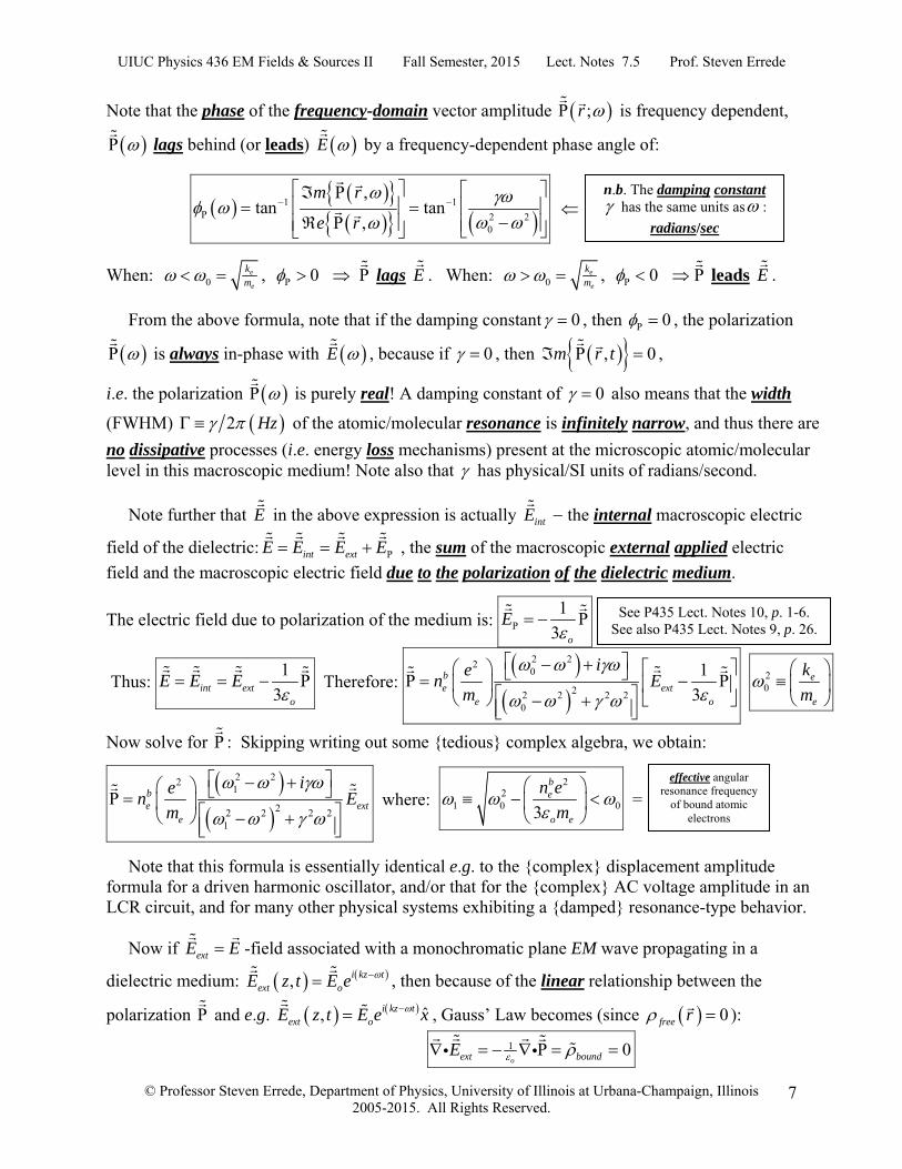
Note that the phase of the frequency-domain vector amplitude ;r is frequency dependent,

lags behind (or leads) E

by a frequency-dependent phase angle of:

1 1

2 20

,tan tan

,

m r

e r

When: 0e

e

km , 0

lags E . When: 0

e

e

km , 0

leads E .

From the above formula, note that if the damping constant 0 , then 0 , the polarization

is always in-phase with E

, because if 0 , then , 0m r t ,

i.e. the polarization is purely real! A damping constant of 0 also means that the width

(FWHM) 2 Hz of the atomic/molecular resonance is infinitely narrow, and thus there are

no dissipative processes (i.e. energy loss mechanisms) present at the microscopic atomic/molecular level in this macroscopic medium! Note also that has physical/SI units of radians/second.

Note further that E in the above expression is actually intE

the internal macroscopic electric

field of the dielectric: Pint extE E E E , the sum of the macroscopic external applied electric

field and the macroscopic electric field due to the polarization of the dielectric medium.

The electric field due to polarization of the medium is: P

1

3 o

E

Thus: 1

3int exto

E E E

Therefore:

2 220

22 2 2 20

1

3be ext

e o

ien E

m

20

e

e

k

m

Now solve for : Skipping writing out some {tedious} complex algebra, we obtain:

2 221

22 2 2 21

be ext

e

ien E

m

where: 2

21 0 03

be

o e

n e

m

=

Note that this formula is essentially identical e.g. to the {complex} displacement amplitude formula for a driven harmonic oscillator, and/or that for the {complex} AC voltage amplitude in an LCR circuit, and for many other physical systems exhibiting a {damped} resonance-type behavior.

Now if extE E -field associated with a monochromatic plane EM wave propagating in a

dielectric medium: , i kz text oE z t E e , then because of the linear relationship between the

polarization and e.g. ˆ, i kz t

ext oE z t E e x , Gauss’ Law becomes (since 0free r

):

1 0oext boundE

See P435 Lect. Notes 10, p. 1-6. See also P435 Lect. Notes 9, p. 26.

effective angular resonance frequency

of bound atomic electrons

n.b. The damping constant has the same units as :

radians/sec



8

The wave equation for a dielectric medium with 0free r and 0freeJ

becomes:

2 22 22 212

2 2 2 222 2 2 21

1 bext extext o o e

e

iE EeE n

c t t m t

with: 2

1o oc

Or:

2 22 212

2 222 2 2 21

11

be ext

exto e

in e EE

c m t

with:

22

1 0 3

be

o e

n e

m

The general solution to this dispersive wave equation is of the form:

, ;i kz t

ext oE r t E e

with complex k k i and:

2 22212

2 22 2 2 21

1be

o e

in ek

c m

.

Thus, we also see that here {again} the complex wavenumber k k i is explicitly

dependent on the angular frequency , i.e. k k i .

We further see that monochromatic plane EM waves propagating in a dispersive dielectric

medium are exponentially attenuated, because: , ;i kz t i kz tz

ext o oE r t E e E e e

,

i.e. the m k term corresponds to absorption/dissipation in the macroscopic

dielectric, and is physically related to/is proportional to the damping constant .

Note that we also have: , , , ,o e extr t E r t , thus the susceptibility e {here} is

also complex, and frequency-dependent: e e ei . The e em term

corresponds to absorption/dissipation in the dielectric, and is physically related to/is proportional to the damping constant . The corresponding dissipative energy losses at the microscopic, atomic/ molecular level in the dielectric ultimately wind up as heat!

Since:

2 221

22 2 2 21

2 221

22 2 2 21

, ; , ; , ;

, ;

bo e ext e ext

e

be

o exto e

ier t E r t n E r t

m

in eE r t

m

where: 2

21 0 3

be

o e

n e

m



9

We see that the complex susceptibility associated with a single resonance is:

2 221

22 2 2 21

be

e e eo e

in ei

m

Hence:

2 221

22 2 2 21

be

e eo e

n ee

m

And:

2

22 2 2 21

be

e eo e

n em

m

Now before we go much further with this, we need to discuss another aspect of our model – namely that in most linear dielectric materials, the atoms comprising the material are multi-electron atoms, and consequently there are many different binding energies – the outer shell

atomic electrons are weakly bound, hence have small ek , and thus small 0 e ek m , whereas

the inner-shell electrons are much more tightly bound, hence have larger ek , larger 0 e ek m .

Furthermore, in complex media, i.e. dielectrics with more than one kind of atom, electrons can be shared between atoms – i.e. they are bound to molecules e.g. the π-electrons in benzene ring / aromatic hydrocarbon-type compounds, which can be weakly bound in some molecules.

Thus, there can be also be {molecular} resonances e.g. in the microwave and infra-red regions of the EM spectrum – atomic resonances are typically in the optical and UV regions {for the outer-most shell electrons}, as well as in the far UV and x-ray regions {for the inner-shell electrons}!

Allowing for all such resonances, we can write the {complex} electric polarization as a

summation over all of the resonances present in the linear dielectric as follows:

2 221

22 2 2 211

, ; , ;b n

j josceo j ext

jo ej j

in er t f E r t

m

where: 2

21 0 3

be

j jo e

n e

m

and: 0e j

je

k

m

and where: oscjf oscillator strength of jth resonance, defined such that:

1

1n

oscj

j

f

Physically: oscjf = fractional strength of the jth resonance and j = 2×width j of the jth resonance.



10

Thus, we see that the multi-resonance complex electric susceptibility e e ei is:

2 221

22 2 2 211

b nj josce

e j e ejo e

j j

in ef i

m

Hence:

2 221

22 2 2 211

b njosce

e e jjo e

j j

n ee f

m

And:

2

22 2 2 211

b njosce

e e jjo e

j j

n em f

m

The complex electric permittivity 1o e i of a dispersive, linear

dielectric medium is:

2 221

22 2 2 211

1 1b n

j josceo e o j

jo ej j

in ef i

m

with the relations:

2 221

22 2 2 211

1 1

1

o e o e

b nj josce

o jjo e

j j

e e

in ef

m

and:

2

22 2 2 211

1

o e o e

b njosce

o jjo e

j j

m m

n ef

m

.



11

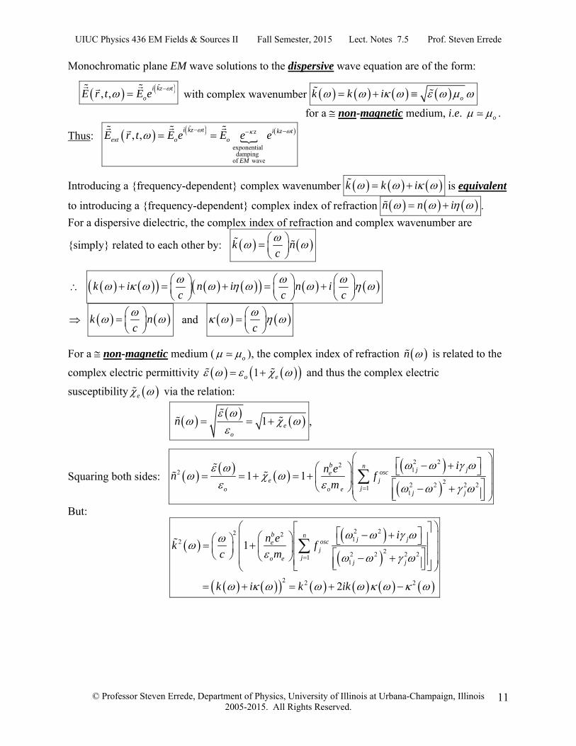
Monochromatic plane EM wave solutions to the dispersive wave equation are of the form:

, ,i kz t

oE r t E e

with complex wavenumber ok k i

for a non-magnetic medium, i.e. o .

Thus:

exponential dampingof wave

, ,i kz t i kz tz

ext o o

EM

E r t E e E e e

Introducing a {frequency-dependent} complex wavenumber k k i is equivalent

to introducing a {frequency-dependent} complex index of refraction n n i .

For a dispersive dielectric, the complex index of refraction and complex wavenumber are

{simply} related to each other by: k nc

k i n i n ic c c

k nc

and c

For a non-magnetic medium ( o ), the complex index of refraction n is related to the

complex electric permittivity 1o e and thus the complex electric

susceptibility e via the relation:

1 eo

n

,

Squaring both sides:

2 2212

22 2 2 211

1 1b n

j joscee j

jo o ej j

in en f

m

But:

2 22 212

22 2 2 211

2 2 2

1

2

b nj josce

jjo e

j j

in ek f

c m

k i k ik



12

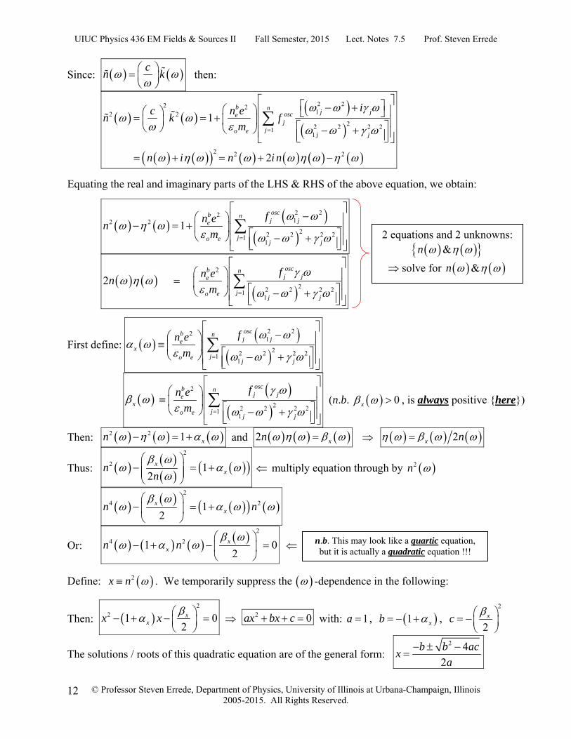
Since: cn k

then:

2 22 212 2

22 2 2 211

2 2 2

1

2

b nj josce

jjo e

j j

in ecn k f

m

n i n i n

Equating the real and imaginary parts of the LHS & RHS of the above equation, we obtain:

2 2212 2

22 2 2 211

1oscb nj je

jo ej j

fn en

m

2

22 2 2 211

2 oscb nj je

jo ej j

fn en

m

First define:

2 221

22 2 2 211

oscb nj je

xjo e

j j

fn e

m

2

22 2 2 211

oscb nj je

xjo e

j j

fn e

m

(n.b. 0x , is always positive {here})

Then: 2 2 1 xn and 2 xn 2x n

Thus:

2

2 12

xxn

n

multiply equation through by 2n

2

4 212

xxn n

Or: 2

4 21 02

xxn n

Define: 2x n . We temporarily suppress the -dependence in the following:

Then: 2

2 1 02

xxx x

2 0ax bx c with: 1a , 1 xb , 2

2xc

The solutions / roots of this quadratic equation are of the general form: 2 4

2

b b acx

a

2 equations and 2 unknowns:

&n

solve for &n

n.b. This may look like a quartic equation, but it is actually a quadratic equation !!!



13

22

2 2

1 1 42 1

1 12 2

xx x

x x xx

i.e.

2

11 1 1

2 1x

xx

x

n.b. the term:

2

01

x

x

Must select +ve root on physical grounds, since 2 0x n .

2

2 11 1 1

2 1x

xx

x n

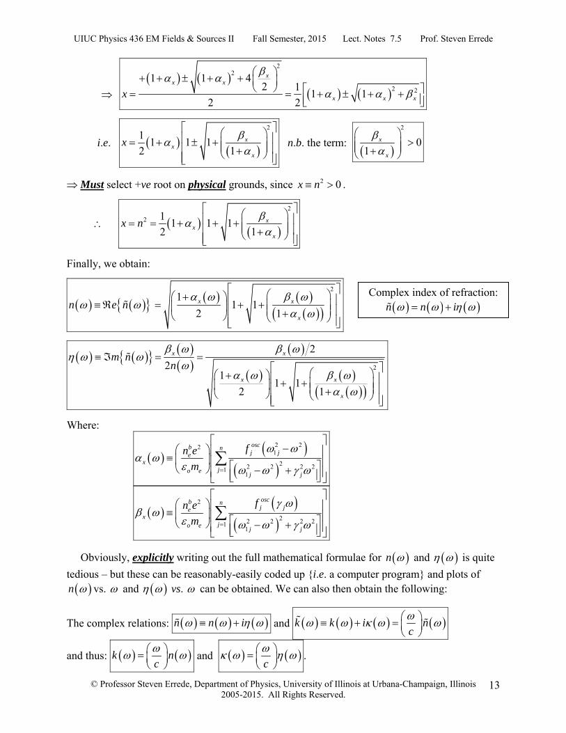
Finally, we obtain:

2

1 1 1

2 1x x

x

n e n

2

2

21

1 12 1

x x

x x

x

m nn

Where:

2 221

22 2 2 211

oscb nj je

xjo e

j j

fn e

m

2

22 2 2 211

oscb nj je

xjo e

j j

fn e

m

Obviously, explicitly writing out the full mathematical formulae for n and is quite

tedious – but these can be reasonably-easily coded up {i.e. a computer program} and plots of

n vs. and vs. can be obtained. We can also then obtain the following:

The complex relations: n n i and k k i nc

and thus: k nc

and c

.

Complex index of refraction:

n n i



14

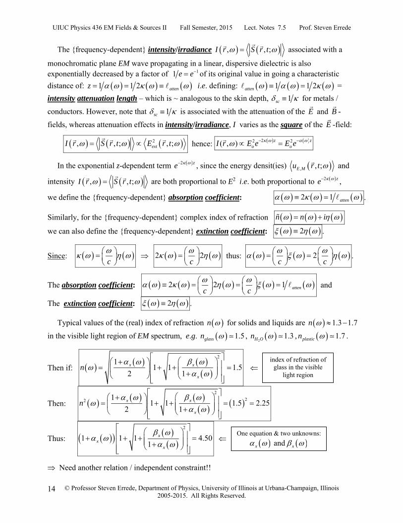
The {frequency-dependent} intensity/irradiance , , ;I r S r t

associated with a

monochromatic plane EM wave propagating in a linear, dispersive dielectric is also exponentially decreased by a factor of 11 e e of its original value in going a characteristic

distance of: 1 1 2 attenz i.e. defining: 1 1 2atten =

intensity attenuation length – which is ~ analogous to the skin depth, 1sc for metals /

conductors. However, note that 1sc is associated with the attenuation of the E

and B

-

fields, whereas attenuation effects in intensity/irradiance, I varies as the square of the E

-field:

2, , ; , ;extI r S r t E r t

hence: 22 2( , ) z zo oI r E e E e

In the exponential z-dependent term 2 ze , since the energy densit(ies) , , ;E Mu r t and

intensity , , ;I r S r t

are both proportional to E2 i.e. both proportional to 2 ze ,

we define the {frequency-dependent} absorption coefficient: 2 1 atten .

Similarly, for the {frequency-dependent} complex index of refraction n n i

we can also define the {frequency-dependent} extinction coefficient: 2 .

Since: c

2 2c

thus: 2c c

.

The absorption coefficient: 2 2 1 attenc c

and

The extinction coefficient: 2 .

Typical values of the (real) index of refraction n for solids and liquids are 1.3 1.7n

in the visible light region of EM spectrum, e.g. 1.5glassn , 2

1.3H On , 1.7plasticn .

Then if:

21

1 1 1.52 1x x

x

n

Then:

2

22 11 1 1.5 2.25

2 1x x

x

n

Thus:

2

1 1 1 4.501

xx

x

Need another relation / independent constraint!!

index of refraction of glass in the visible

light region

One equation & two unknowns:

and x x



15

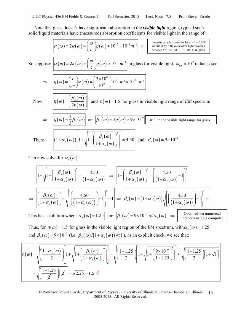
Note that glass doesn’t have significant absorption in the visible light region, typical such solid/liquid materials have (measured) absorption coefficients for visible light in the range of:

2 1 12 10 10 mc

So suppose: 1 12 10 mc

in glass for visible light, 1610 radians / secvis

8

1 916

3 1010 3 10 1

10

c

Now: 2

x

n

and 1.5n for glass in visible light range of EM spectrum.

1

3 x or: 93 9 10x

Then:

2

1 1 1 4.501

xx

x

and: 99 10x .

Can now solve for x :

2

4.501 1

1 1x

x x

22

4.501 1

1 1x

x x

2

4.501 1

1 1x

x x

2

4.501 1 1

1x xx

This has a solution when: 1.25x for: 99 10x x

Thus, for 1.5n for glass in the visible light region of the EM spectrum, with 1.25x

and 99 10x (i.e. 1 1x x ), as an explicit check, we see that:

2 291 1 1.25 9 10 1 1.251 1 1 1 1 1

2 1 2 1 1.25 2

1 1.25

2

x x

x

n

2

2.25 1.5

Intensity I(z) decreases to 1/e = e–1 = 0.368 of initial I(z = 0) value after light travels a distance z = 1/ () ~ 10 – 100 m in glass.

Obtained via numerical methods using a computer

1 in the visible light range for glass



16

Thus we also see that:

2 2212

22 2 2 211

1oscb nj je

xjo e

j j

fn en

m

i.e. 2 1 xn

for typical materials – glass, water, plastic – in the visible light region of the EM spectrum, 1610 radians / sec .

Whereas:

2

22 2 2 211

1oscb nj je

xjo e

j j

fn e

m

for these same materials – glass, water, plastic – in the visible light region of the EM spectrum, 1610 radians / sec .

Our original equations were: 2 2 1 xn and 2 xn or:

2x n with: 1.25x and 99 10x for 1.5n (for glass)

with visible light and: 92 3 10x n .

We now see more clearly that: n in the visible light region of the EM spectrum

for glass, i.e. the complex index of refraction 91.25 9 10n n i i for glass is

predominantly real in the visible light region of the EM spectrum.

Thus, for glass in the visible light region of the EM spectrum:

2 22

22 2 2

22 2 2 211

1 1 1.5 2.25oscb nj je

xjo

j j

fn en n

m

and:

29

22 2 2 2101

2 9 10oscb nj je

xj

j j

fn en

m

2 22

22 2 2 211

1.25oscb nj je

xjo

j j

fn e

m

Note that these results that we just obtained for glass in the visible light region of the EM spectrum do not hold true for all frequencies of EM waves {visible light region is in fact only a narrow portion of the EM spectrum}!!! In particular, these results do not hold at {or near} an atomic (or molecular) resonance!



17

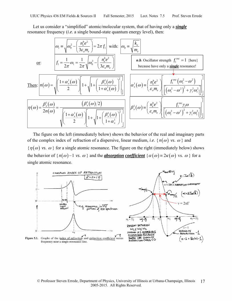
Let us consider a “simplified” atomic/molecular system, that of having only a single resonance frequency (i.e. a single bound-state quantum energy level), then:

22

1 0 123

be

o e

n ef

m

with: 0e

e

k

m

or: 2

21 1 0

1 1

2 2 3

be

o e

n ef

m

Then:

21 1

1

11 1

2 1x x

x

n

2 221 11

22 2 2 21 1 1

oscbe

xo e

fn e

m

11

21 1

1

2

21

1 12 1

xx

x x

x

n

21 1 1

22 2 2 21 1 1

b osce

xo e

n e f

m

The figure on the left (immediately below) shows the behavior of the real and imaginary parts of the complex index of refraction of a dispersive, linear medium, i.e. { n vs. } and

{ vs. } for a single atomic resonance. The figure on the right (immediately below) shows

the behavior of { 1n vs. } and the absorption coefficient { 2 vs. } for a

single atomic resonance.

n.b. Oscillator strength 1 1oscf {here}

because have only a single resonance!

= 2



18

1 0 n

= o

= 0 =

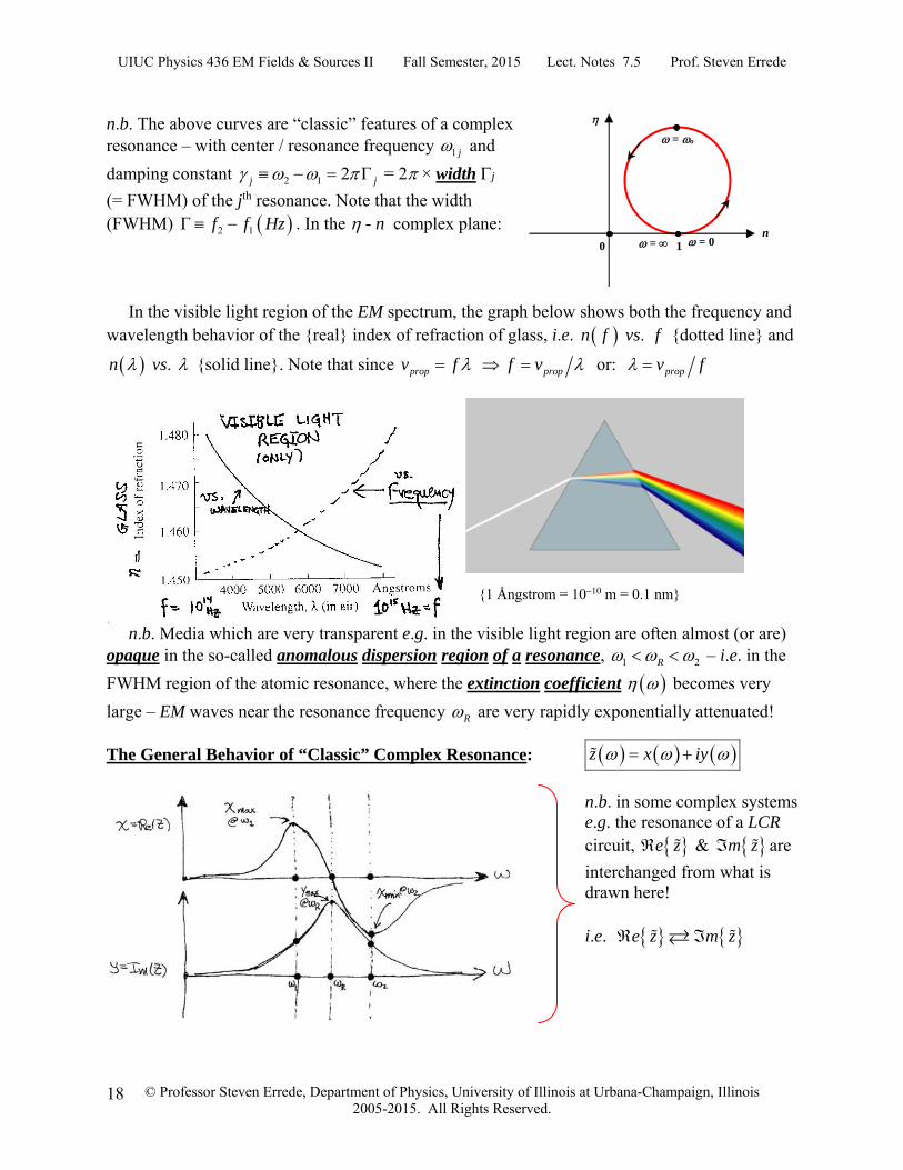
n.b. The above curves are “classic” features of a complex resonance – with center / resonance frequency 1 j and

damping constant 2 1 2 Γj j = 2 × width j

(= FWHM) of the jth resonance. Note that the width (FWHM) 2 1Γ f f Hz . In the - n complex plane:

In the visible light region of the EM spectrum, the graph below shows both the frequency and wavelength behavior of the {real} index of refraction of glass, i.e. n f vs. f {dotted line} and

n vs. {solid line}. Note that since propv f propf v or: propv f

{1 Ångstrom = 1010 m = 0.1 nm} n.b. Media which are very transparent e.g. in the visible light region are often almost (or are) opaque in the so-called anomalous dispersion region of a resonance, 1 2R – i.e. in the

FWHM region of the atomic resonance, where the extinction coefficient becomes very

large – EM waves near the resonance frequency R are very rapidly exponentially attenuated!

The General Behavior of “Classic” Complex Resonance: z x iy

n.b. in some complex systems e.g. the resonance of a LCR circuit, e z & m z are

interchanged from what is drawn here! i.e. e z m z



19

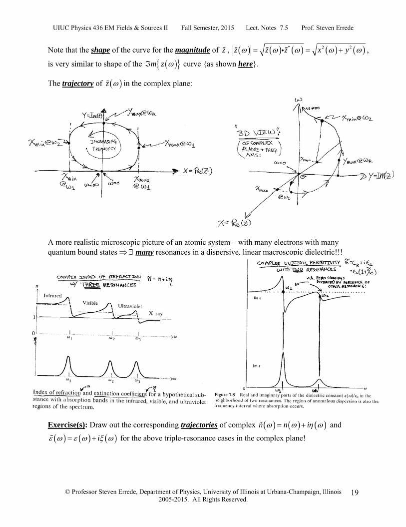
Note that the shape of the curve for the magnitude of z , * 2 2z z z x y ,

is very similar to shape of the m z curve {as shown here}.

The trajectory of z in the complex plane:

A more realistic microscopic picture of an atomic system – with many electrons with many quantum bound states many resonances in a dispersive, linear macroscopic dielectric!!!

Exercise(s): Draw out the corresponding trajectories of complex n n i and

i for the above triple-resonance cases in the complex plane!



20

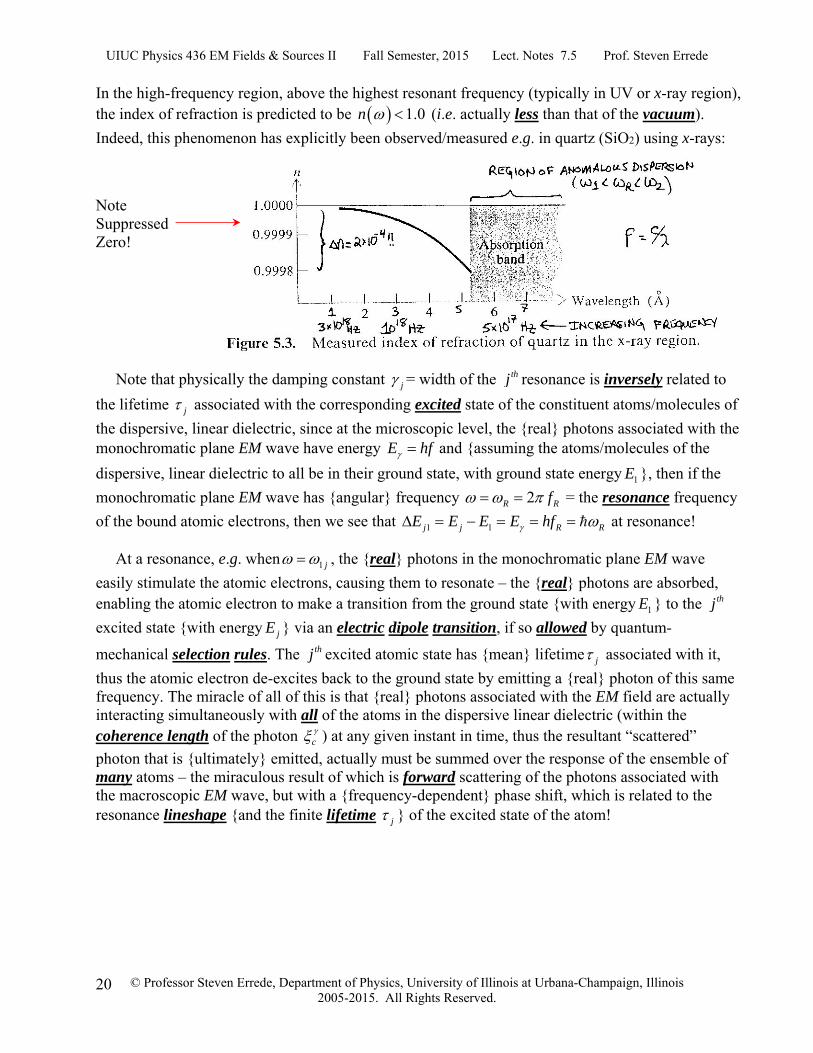
In the high-frequency region, above the highest resonant frequency (typically in UV or x-ray region), the index of refraction is predicted to be 1.0n (i.e. actually less than that of the vacuum).

Indeed, this phenomenon has explicitly been observed/measured e.g. in quartz (SiO2) using x-rays:

Note Suppressed Zero!

Note that physically the damping constant j = width of the thj resonance is inversely related to

the lifetime j associated with the corresponding excited state of the constituent atoms/molecules of

the dispersive, linear dielectric, since at the microscopic level, the {real} photons associated with the monochromatic plane EM wave have energy E hf and {assuming the atoms/molecules of the

dispersive, linear dielectric to all be in their ground state, with ground state energy 1E }, then if the

monochromatic plane EM wave has {angular} frequency 2R Rf = the resonance frequency

of the bound atomic electrons, then we see that 1 1j j R RE E E E hf at resonance!

At a resonance, e.g. when 1 j , the {real} photons in the monochromatic plane EM wave

easily stimulate the atomic electrons, causing them to resonate – the {real} photons are absorbed, enabling the atomic electron to make a transition from the ground state {with energy 1E } to the thj

excited state {with energy jE } via an electric dipole transition, if so allowed by quantum-

mechanical selection rules. The thj excited atomic state has {mean} lifetime j associated with it,

thus the atomic electron de-excites back to the ground state by emitting a {real} photon of this same frequency. The miracle of all of this is that {real} photons associated with the EM field are actually interacting simultaneously with all of the atoms in the dispersive linear dielectric (within the coherence length of the photon c

) at any given instant in time, thus the resultant “scattered”

photon that is {ultimately} emitted, actually must be summed over the response of the ensemble of many atoms – the miraculous result of which is forward scattering of the photons associated with the macroscopic EM wave, but with a {frequency-dependent} phase shift, which is related to the resonance lineshape {and the finite lifetime j } of the excited state of the atom!



21

At a resonance, e.g. when 1k , a large, transitory/transient {complex and frequency-

dependent} electric dipole moment ˆ,p r er er r is induced in the atom, where:

2 221

22 2 2 211

b nj josce

o jjo e

j j

in er r f r i

m

Note here we can also make a direct connection with quantum mechanics – the electric dipole

moment operator , p r e r and position operator r operating e.g. on the ground

state wave function of the atom/molecule 1 r , i.e. 1,p r r and 1r r .

We can e.g. compute the expectation value of the modulus squared of the electric dipole

moment 2

1 1,r p r r of the atom/molecule. Inserting a complete set of states

1 1

1j j j jj j

r r r r

into this expression, we can then obtain the quantum

mechanical predictions for the {squares} the oscillator strengths oscjf :

2

*1 1 1

1 1

, , ,j j jj j

r p r r r p r r r p r r

The transition rate 1 j

(= # atoms/molecules per second) from the ground state to the thj

excited state {via an electric dipole transition, as allowed by quantum mechanical selection rules}

is proportional to 1,j r p r r , whereas the transition rate 1j

(= # atoms/ molecules

per second) from the thj excited state to the ground state {via an electric dipole transition, as

allowed by quantum mechanical selection rules} is proportional to *1 , jr p r r .

Note that by the {microscopic} manifest time-reversal invariance of the electromagnetic interaction, the transition rates are identical, i.e.

1 12jj j

= “damping constant”

in our semi-classical model!

Note further that the lifetimes j of the excited states of atoms are {inversely} related to the

widths j of the thj resonances/widths of the thj excited states by the Heisenberg uncertainty

principle: E t , where 2h and h = Planck’s constant. If we set this relation to its minimum, i.e. E t then:

j j j j or: 1 11 2j jj j



22

If one stays well away/far from {all} of the resonance frequencies of bound-state atomic electrons, the resonance factor becomes:

2 2

1 j ji

22 2 2 21 j j

2 21

1

j

i.e. far from a resonance: 2 21 j j

Thus, far from a resonance / all resonances, relatively little absorption/dissipation occurs {i.e. 2 2n , such that n n n is predominantly real} and hence:

2

2 2 22 2

1 1

1oscb nje

jo e j

fn en n

m

Now:

2 2 21

2 2 2 2 2 42 21 1 1 1 11

11 1 11

1

j

j j j j jj

Then: 2

2 2 2 22 4

1 11 1

1osc oscb n nj je

j jo e j j

f fn en n

m

If 2 1n and 1 121 1n

Thus, far from a resonance/resonances: 2

22 4

1 1

11

2

osc oscb n nj je

j jo e j j

f fn en

m

But: 2 2

oo

c

k

= vacuum wavelength, hence: 2

o

c

, thus:

22

2 41 1

1 21

2

osc oscb n nj je

oj jo e j o j

f fn e cn

m

we obtain Cauchy’s Formula: 21 1o

o

Bn A

Where: A = Coefficient of Refraction and: B = Coefficient of Dispersion.

Comparing the 2 equations, we see that:

2

21

1

2

oscb nje

jo e j

fn eA

m

and: 2

4 21 1

2osc oscn nj j

j jj j

f fB c



23

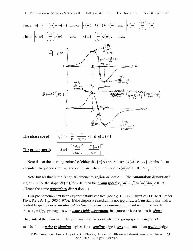
Since: n n i and/or: k k ik and: k nc

Then: k nc

and: c

, thus:

The phase speed: c

v ck n

if n < 1

The group speed: 1" "

g

dkdv

dk d

Note that at the “turning points” of either the { n vs. } or: { k vs. } graphs, i.e. at

{angular} frequencies 1 and/or 2 where the slope 0dk d gv !!!

Note further that in the {angular} frequency region 1 2 {the “anomalous dispersion”

region}, since the slope 0dk d then the group speed 1 0gv dk d !!!

{Hence the name anomalous dispersion…}

This phenomenon has been experimentally verified (see e.g. C.G.B. Garrett & D.E. McCumber, Phys. Rev. A, 1, p. 305 (1970). If the dispersive medium is not too thick, a Gaussian pulse with a central frequency near an absorption line (i.e. near a resonance, R ) and with pulse width

1R Rt propagates with appreciable absorption, but (more or less) retains its shape.

The peak of the Gaussian pulse propagates at vg even when the group speed is negative!!!

Useful for pulse re-shaping applications - leading edge is less attenuated than trailing edge.

1



24

Can actually have the peak of a greatly attenuated pulse emerge from the absorber before the peak of the incident pulse enters the absorber ( definition of negative group speed)!!! {i.e. microscopically, if the absorber is not too thick, then some photons can make it all the way through the absorber w/o interacting at all – this probability is exponentially suppressed.

Has applications/uses e.g. in optical mammography/breast cancer screening for women...}

See e.g. J.D. Jackson’s Electrodynamics, 3rd Edition, pages 325-26 for more details! Finally, if we set 0 , then we obtain the static (i.e. zero-frequency) limit of {all of} these quantities. Note that they also {all} become purely real in this limit:

Static Polarization: 2

21 1

(0)oscb nje

j j

fn e

m

where

22

1 0 3j

be

jo e

n e

m

and since o e extE

Static Electricity Susceptibility: 2

21 1

(0)oscb nje

ejo e j

fn e

m

and 0 j

e j

e

k

m

Static Index of Refraction: 0 1 0 1 (0) (0)x e en K

But: 1e o eK 0 1 0o e and thus:

Static Dielectric Constant: 20 0 1 0 1 0 0e o e xK n

But: 2

21 1

0 0oscb nje

x ejo e j

fn e

m

2

22

1 1

0 1 0oscb nje

ejo e j

fn eK n

m

and:

2

21 1

0 0 1oscb nje

e ejo e j

fn eK

m

Note that the static dielectric constant {as measured at f = 0 Hz/DC} is 0 1.0eK because it

contains information about all of the {quantum mechanical} resonances/excited states 1 0j

present in the dispersive, linear medium, even into the x-ray region at 18 191 10j Hz and beyond !!!

Equivalently, armed now with this knowledge of the microscopic behavior of a dispersive, linear medium, an electric susceptibility 0e > 0 {or equivalently, a dielectric constant

0eK >1} instantly tells us that there are indeed {quantum mechanical} resonances/excited

states present in the {composite} atoms/molecules that make up the macroscopic material of the dispersive, linear medium!!!



25

A wonderful macroscopic example of dispersion in nature is the rainbow. At the microscopic level, the frequency-dependence of the index of refraction of light n() arises as a consequence of the resonant behavior of quantum mechanical bound states of electrons in the atoms of the water molecule (H2O) responding to EM light waves{= visible light photons} coming from our sun. If no such composite behavior existed at the microscopic level, there would be no rainbows to enjoy in the macroscopic everyday world!

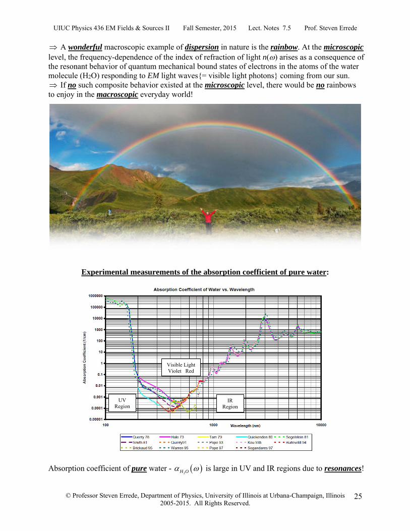
Experimental measurements of the absorption coefficient of pure water:

Absorption coefficient of pure water - 2H O is large in UV and IR regions due to resonances!

Visible Light Violet Red

UV Region

IR Region

lecture notes 7 - high energy physics at the...

Documents