lecture notes fourier analysis - university of washington

Lecture NotesFourier Analysis

Prof. Xu ChenDepartment of Mechanical Engineering

University of Washingtonchx AT uw.edu

X. Chen Fourier Analysis September 29, 2019

Contents

1 Background 11.1 Periodic functions . . . . . . . . . . . . . . . . . . . . . . . . . . . . . . . . . . . . . 11.2 Orthogonal decomposition . . . . . . . . . . . . . . . . . . . . . . . . . . . . . . . . . 1

2 Fourier series 32.1 Arbitrary period . . . . . . . . . . . . . . . . . . . . . . . . . . . . . . . . . . . . . . 42.2 Even and odd functions . . . . . . . . . . . . . . . . . . . . . . . . . . . . . . . . . . 52.3 Application example: ODE with special inputs . . . . . . . . . . . . . . . . . . . . . . 6

3 Complex Fourier series 7

4 Fourier integral 8

5 Fourier transform 10

6 *Discrete Fourier analysis 116.1 Discrete Fourier series . . . . . . . . . . . . . . . . . . . . . . . . . . . . . . . . . . . 116.2 Discrete-time Fourier transform (DTFT) . . . . . . . . . . . . . . . . . . . . . . . . . 126.3 Discrete Fourier transform (DFT) . . . . . . . . . . . . . . . . . . . . . . . . . . . . . 13


Notations:If x is complex, < (x) and = (x) denote, respectively, the real and imaginary parts of x.〈x, y〉 denotes the inner product of x and y.

1 Background

Fourier analysis is important in modeling and solving partial differential equations related to boundaryand initial value problems of mechanics, heat flow, electrostatics, and other fields.

1.1 Periodic functions

A function f(x) is called periodic if f(x) is defined for all real x, except possibly at some points, andif there is some positive number p, called a period of f(x), such that

f (x+ p) = f (x)

Remark 1. If p is a period of f(x), then clearly 2p, 3p, . . . are also periods of f (x).

The smallest positive period is called the fundamental period.

1.2 Orthogonal decomposition

In vector spaces equipped with inner products, we have the following essential theorem.

Theorem 2. Suppose {e1, e2, . . . , en} is an orthogonal basis of a vector space V. Then for everyv ∈ V, we have

v =〈v, e1〉〈e1, e1〉

e1 + · · ·+ 〈v, en〉〈en, en〉

en

or, by using the norm notation,

v =〈v, e1〉||e1||2

e1 + · · ·+ 〈v, en〉||en||2

en

Proof. Let v ∈ V. Because {e1, e2, . . . , en} is a basis, there exists scalars α1, . . . , αn such that

v = α1e1 + · · ·+ αnen

Taking the inner product with ej (j = 1, . . . , n) yields

〈v, ej〉 = 〈α1e1 + · · ·+ αnen, ej〉 = α1 〈e1, ej〉+ · · ·+ αn 〈en, ej〉

But the basis is orthogonal, hence 〈ei, ej〉 = 0 if i 6= j. This yields

〈α1e1 + · · ·+ αnen, ej〉 = αj 〈ej, ej〉

1


and thus〈v, ej〉 = αj 〈ej, ej〉 ⇐⇒ αj =

〈v, ej〉〈ej, ej〉

Recall that we have the following fact.

Fact (Inner product for functions, function spaces). The set of all real-valued continuous functionsf (x), g (x), . . . x ∈ [α, β] is a real vector space under the usual addition of functions and multiplicationby scalars. An inner product on this function space is

〈f, g〉 =

∫ β

α

f (x) g (x) dx

and the norm of f is

||f (x) || =

√∫ β

α

f (x)2 dx

As a very useful special case, the trigonometric system is a function space with orthogonal basis{sinnx, cosnx, 1}∞n=1. To check, we first notice that the functions are all periodic with period 2π. Theinner product in this case is

〈f, g〉 =

∫ π

−πf (x) g (x) dx

Noting that, by checking the area under the graphs and noting the shape of sine and cosine functions,we have ∫ π

−πcosnxdx = 0, ∀n = 1, 2, . . . (1)∫ π

−πsinnxdx = 0, ∀n = 1, 2, . . .

This confirms the orthogonality between 1 and sinnx or cosnx. Furthermore, using (1) we immediatelyknow

〈cosnx, cosmx〉 =

∫ π

−πcosnx cosmxdx =

∫ π

−π

cos (n+m)x+ cos (n−m)x

2dx

=1

2

∫ π

−πcos (n+m)xdx+

1

2

∫ π

−πcos (n−m)xdx

= 0 + 0 as long as n 6= m

namely, cosnx and cosmx are orthogonal if m 6= n.Similarly, as long as n 6= m (by assumption, both m and n are positive integers), sinnx and sinmx

are orthogonal. This is because

〈sinnx, sinmx〉 =

∫ π

−πsinnx sinmxdx =

∫ π

−π

cos (n−m)x− cos (n+m)x

2dx = 0

2


Furthermore, regardless of the values of m and n, we have

〈sinnx, cosmx〉 =

∫ π

−πsinnx cosmxdx =

∫ π

−π

sin (n+m)x+ sin (n−m)x

2dx = 0

So sinnx and cosmx are always orthogonal.Sketch the plots of sine and cosine functions. You should find the above results intuitive.To perform the orthogonal decomposition under the trigonometric system, we need just one more

thing–the norms of the basis functions. They are

|| sinnx||2 = 〈sinnx, sinnx〉 =

∫ π

−π(sinnx)2 dx =

∫ π

−π

1− cos 2nx

2dx = π

|| cosnx||2 =

∫ π

−π(cosnx)2 dx =

∫ π

−π

cos 2nx+ 1

2dx = π

||1||2 =

∫ π

−π1dx = 2π

2 Fourier series

Fourier series is an extension of the orthogonal decomposition reviewed in the last section. Under thetrigonometric system, the orthogonal decomposition of a function f (x)—provided that the decompo-sition exists (we will talk about the existence very soon)—is

f (x) = a0 +∞∑n=1

(an cosnx+ bn sinnx) (2)

wherea0 =

〈f (x) , 1〉〈1, 1〉

=1

2π

∫ π

−πf (x) dx (3)

and

an =〈f (x) , cosnx〉〈cosnx, cosnx〉

=1

π

∫ π

−πf (x) cosnxdx, bn =

〈f (x) , sinnx〉〈sinnx, sinnx〉

=1

π

∫ π

−πf (x) sinnxdx (4)

(2) is called the Fourier series of f (x). (3) and (4) are called the corresponding Fourier coefficients.

Example 3. Find the Fourier coefficients of

f (x) =

{−k if − π < x < 0

k if 0 < x < π, and f (x+ 2π) = f (x)

Such functions occur as external forces acting on mechanical systems, electromotive forces in electriccircuits, etc.

3


(Solution:

f (x) =4k

π

(sinx+

1

3sin 3x+

1

5sin 5x+ . . .

))

Theorem 4 (Existance of Fourier Series). Let f (x) be periodic with period 2π and piecewise continuousin the interval −π ≤ x ≤ π. Furthermore, let f (x) have a left-hand derivative and a right-handderivative at each point of that interval. Then the Fourier series of f (x) converges. Its sum is f (x),except at points xo where f (x) is discontinuous. There the sum of the series is the average of the left-and right-hand limits of f (x) at xo.

Hence a periodic function f (x) = f (x+ 2π) with

f (x) = 1/x, x ∈ [−π, π]

does not have a Fourier series extension, as it does not have a left- or right-hand derivative at x = 0.A discontinuous periodic function, with period 2π and

f (x) =

{1, −π < x < 0

−1, π > x ≥ 0

is piecewise continuous. At x = 0, it has a left-hand derivative of 0 and a right-hand derivative of 0.Hence the function has a Fourier series expansion.

2.1 Arbitrary period

The transition from period 2π to period p = 2L can be done by a suitable change of scale. If f (x) hasa period 2L, we let

v =x

Lπ

You can see, that x = ±L corresponds to v = ±π. So

f (x) = f

(L

πv

)is periodic in v with period 2π.

Now forget about f (x). Focus just on the new f(Lπv)with period 2π. The Fourier series is

f

(L

πv

)= a0 +

∞∑n=1

(an cosnv + bn sinnv)

where

a0 =1

2π

∫ π

−πf

(L

πv

)dv, an =

1

π

∫ π

−πf

(L

πv

)cosnvdv, bn =

1

π

∫ π

−πf

(L

πv

)sinnvdv (5)

4


Changing back to the x notation, by using

f (x) = f

(L

πv

), v =

x

Lπ, dv =

π

Ldx

we have

f (x) = a0 +∞∑n=1

(an cos

nπ

Lx+ bn sin

nπ

Lx)

(6)

with

a0 =1

2L

∫ L

−Lf (x) dx, an =

1

L

∫ L

−Lf (x) cos

nπ

Lxdx, bn =

1

L

∫ L

−Lf (x) sin

nπ

Lxdx (7)

Example 5. Find the Fourier series of

f (x) =

0 if − 2 < x < −1

k if − 1 < x < 1

0 if 1 < x < 2

, p = 2L = 4, L = 2

Answer:

f (x) =k

2+

2k

π

(cos

π

2x− 1

3cos

3π

2x+

1

5cos

5π

2x−+ . . .

)

2.2 Even and odd functions

It turns out that, if f(x) is even or odd, the Fourier series can be significantly simplified. This isbecause, if f (x) is an even function, then∫ L

−Lf (x) sinnxdx = 0

as the integral of any odd function is zero. Hence in (7) bn = 0 so that (6) simplifies to

f (x) = a0 +∞∑n=1

an cosnπ

Lx

Furthermore, since f (x) is even, we have

a0 =1

2L

∫ L

−Lf (x) dx =

1

L

∫ L

0

f (x) dx, an =1

L

∫ L

−Lf (x) cos

nπ

Lxdx =

2

L

∫ L

0

f (x) cosnπ

Lxdx

Similarly, if f (x) is an odd function, then∫ L

−Lf (x) cosnxdx = 0

5


and

f (x) =∞∑n=1

bn sinnπ

Lx, bn =

2

L

∫ L

0

f (x) sinnπ

Lxdx

The following Theorem is intuitive and very useful.

Theorem 6. The Fourier series of a sum f1 +f2 are the sums of the corresponding Fourier coefficientsof f1 and f2. The Fourier coefficients of cf are c times the corresponding Fourier coefficients of f .

Here is one example of using the results in this subsection.

Example 7 (Sawtooth wave). Find the Fourier series of the function

f (x) = x+ π if − π < x < π and f (x+ 2π) = f (x)

The basic idea is to decompose the function as

f (x) = f1 (x) + f2 (x) , f1 (x) = x, f2 (x) = π

f1 (x) is an odd function; f2 (x) is an even function. Their Fourier coefficients are simpler to find.

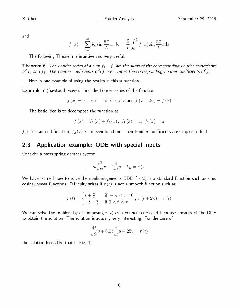
2.3 Application example: ODE with special inputs

Consider a mass spring damper system

md2

dt2y + b

d

dty + ky = r (t)

We have learned how to solve the nonhomogeneous ODE if r (t) is a standard function such as sine,cosine, power functions. Difficulty arises if r (t) is not a smooth function such as

r (t) =

{t+ π

2if − π < t < 0

−t+ π2

if 0 < t < π, r (t+ 2π) = r (t)

We can solve the problem by decomposing r (t) as a Fourier series and then use linearity of the ODEto obtain the solution. The solution is actually very interesting. For the case of

d2

dt2y + 0.05

d

dty + 25y = r (t)

the solution looks like that in Fig. 1.

6

X. Chen Fourier Analysis September 29, 2019494 CHAP. 11 Fourier Analysis

1. Coefficients . Derive the formula for from and

2. Change of spring and damping. In Example 1, whathappens to the amplitudes if we take a stiffer spring,say, of ? If we increase the damping?

3. Phase shift. Explain the role of the ’s. What happensif we let ?

4. Differentiation of input. In Example 1, what happensif we replace with its derivative, the rectangular wave?What is the ratio of the new to the old ones?

5. Sign of coefficients. Some of the in Example 1 arepositive, some negative. All are positive. Is thisphysically understandable?

6–11 GENERAL SOLUTIONFind a general solution of the ODE with

as given. Show the details of your work.6.7.8. Rectifier. and

9. What kind of solution is excluded in Prob. 8 by?

10. Rectifier. and

11.

12. CAS Program. Write a program for solving the ODEjust considered and for jointly graphing input and outputof an initial value problem involving that ODE. Apply

r (t) ! b"1 if "p # t # 0

1 if 0 # t # p, ƒv ƒ $ 1, 3, 5, Á

r (t % 2p) ! r (t), ƒv ƒ $ 0, 2, 4, Ár (t) ! p/4 ƒ sin t ƒ if 0 # t # 2p

ƒv ƒ $ 0, 2, 4, Á

r (t % 2p) ! r (t), ƒv ƒ $ 0, 2, 4, Ár (t) ! p/4 ƒ cos t ƒ if "p # t # p

r (t) ! sin t, v ! 0.5, 0.9, 1.1, 1.5, 10r (t) ! sin at % sin bt, v2 $ a2, b2

r (t)ys % v2y ! r (t)

Bn

An

Cn

r (t)

c : 0Bn

k ! 49Cn

Bn.AnCnCn the program to Probs. 7 and 11 with initial values of your

choice.

13–16 STEADY-STATE DAMPED OSCILLATIONSFind the steady-state oscillations of with and as given. Note that the spring constantis . Show the details. In Probs. 14–16 sketch .

13.

14.

15.

16.

17–19 RLC-CIRCUITFind the steady-state current in the RLC-circuit inFig. 275, where F and with

V as follows and periodic with period . Graph orsketch the first four partial sums. Note that the coefficientsof the solution decrease rapidly. Hint. Remember that theODE contains , not , cf. Sec. 2.9.

17. E (t) ! b"50t 2 if "p # t # 0

50t 2 if 0 # t # p

E (t)Er(t)

2pE (t)R ! 10 &, L ! 1 H, C ! 10!1

I (t)

e t if "p>2 # t # p>2p " t if p>2 # t # 3p>2 and r (t % 2p) ! r (t)

r (t) !

r (t % 2p) ! r (t)r (t) ! t (p2 " t 2) if "p # t # p and

r (t) ! b"1 if "p# t # 0

1 if 0 # t #p and r (t % 2p) ! r (t)

r (t) ! aN

n!1

(an cos nt % bn sin nt)

r (t)k ! 1r (t)c ' 0

ys % cyr % y ! r (t)

P R O B L E M S E T 1 1 . 3

y

t0 1 2 3–1–2–3

0.1

–0.1

–0.2

0.2

0.3

Output

Input

Fig. 277. Input and steady-state output in Example 1

c11-a.qxd 10/30/10 1:25 PM Page 494

Figure 1: Fig. 277 from [EK]

3 Complex Fourier series

Instead of sin and cos functions, we can use {ejnx}∞j=−∞ as the (complex) basis for Fourier series. Forbetter physical intuitions, we usually write n = ωsl. The formula for Fourier series (when it exists) is

f (x) =∞∑

l=−∞

⟨f (x) , ejωslx

⟩〈ejωslx, ejωslx〉

ejωslx (8)

Fact (Inner product for complex functions). The set of all complex-valued continuous functions f (x),g (x), . . . x ∈ [α, β] is a complex vector space under the usual addition of functions and multiplicationby scalars. An inner product on this function space is

〈g, f〉 =

∫ β

α

g (x)f (x) dx

and the norm of f is

||f (x) || =√〈f, f〉 =

√∫ β

α

|f (x)|2 dx

Fact 8. ejωslx has a norm of√Ts =

√2π/ωs

Proof. By definition

||ejωslx|| =√〈ejωslx, ejωslx〉 =

√∫ Ts/2

−Ts/2|ejωslx|2 dx =

√∫ Ts/2

−Ts/2dx =

√Ts

The Fourier series expansion (8) hence simplifies to

f (x) =1

Ts

∞∑l=−∞

⟨f (x) , ejωslx

⟩ejωslx

7


Example 9 (Fourier series of an impulse train). Show that

∞∑l=−∞

δ (t− lTs) =1

Ts

∞∑l=∞

ejωslt, ωs =2π

Ts

where δ (x) is the Kronecker-delta function satisfying δ (x) = 1 if x = 0 and δ (x) = 0 otherwise.∑∞l=−∞ δ (t− lTs) is periodic with period Ts. You can check that ejωst also has a period of Ts if

ωs = 2π/Ts.For the Fourier coefficients, we have

⟨f (t) , ejωslt

⟩=

∫ Ts/2

−Ts/2δ (t) ejωsltdt = 1

Hence∞∑

l=−∞

δ (t− lTs) =1

Ts

∞∑l=−∞

⟨f (x) , ejωslt

⟩ejωslt =

1

Ts

∞∑l=∞

ejωslt, ωs =2π

Ts

4 Fourier integral

What can be done to extend the method of Fourier series to nonperiodic functions? This is the idea of“Fourier integrals.”

Let us consider an example of

f(x) =

{1 if −1 < x < −1

0 otherwise(9)

This is not a periodic function. Construct a rectangular wave

fL(x) =

0 if −L < x < −1

1 if −1 < x < −1

0 if 1 < x < L

, fL (x+ 2L) = fL(x)

We are going to make L increase from some small numbers to infinity, which recovers (9).The function is even. The Fourier coefficients are

a0 =1

2L

∫ 1

−1dx =

1

L, an =

1

L

∫ 1

−1cos

nπx

Ldx =

2

L

∫ 1

0

cosnπx

Ldx =

2

L

sin (nπ/L)

nπ/L

As L increases, the frequency of sin (nπ/L) increases.More generally, consider any periodic function fL (x) of period 2L that can be represented by

fL (x) = a0 +∞∑n=1

[an cosωnx+ bn sinωnx] , ωn =nπ

L

8


where

a0 =1

2L

∫ L

−Lf (x) dx, an =

1

L

∫ L

−Lf (x) cos

nπ

Lxdx, bn =

1

L

∫ L

−Lf (x) sin

nπ

Lxdx

or, in the notation of the newly introduced ωn = nπ/L:

fL (x) =1

2L

∫ L

−LfL (v) dv +

1

L

∞∑n=1

[cosωnx

∫ L

−LfL (v) cosωnvdv + sinωnx

∫ L

−LfL (v) cosωnvdv

](10)

Notice that if we define∆ω = ωn+1 − ωn =

π

L⇒ 1

L=

∆ω

πthen (10) is actually

fL (x) =1

2L

∫ L

−LfL (v) dv

+1

π

∞∑n=1

[∆ω cos (ωnx)

∫ L

−LfL (v) cosωnvdv + ∆ω sin (ωnx)

∫ L

−LfL (v) cosωnvdv

](11)

We want to have an understanding of the case when L→∞. Assume that f (x) = limL→∞ fL (x)is absolutely integrable, i.e. the following finite limit exists

lima→−∞

∫ 0

a

|f (x)| dx+ limb→∞

∫ b

0

|f (x)| dx

Then

limL→∞

1

2L

∫ L

−LfL (v) dv = 0

Let g (ω) = cos (ωx)∫ L−L fL (v) cosωvdv. The first summation in (11) is

∞∑n=1

∆ωg (ωn) = g (ω1) ∆ω + g (ω2) ∆ω + . . .

As ∆ω = π/L→ 0 if L→∞, the last term in (11) thus looks like an integration

f (x) =1

π

∫ ∞0

[cosωx

∫ ∞−∞

f (v) cosωvdv + sinωx

∫ ∞−∞

f (v) cosωvdv

]dω

Letting

A (ω) =1

π

∫ ∞−∞

f (v) cosωvdv, B (w) =1

π

∫ ∞−∞

f (v) sinωvdv

yields

f (x) =

∫ ∞0

[A (ω) cosωx+B (ω) sinωx] dω

This is called a representation of f (x) (no longer periodic) by a Fourier integral.

9


Remark 10. The above construction is only an intuition. Nonetheless, the conclusion is correct.

Theorem 11 (Existance of Fourier Integral). If f (x) is piecewise continuous in every finite intervaland has a right hand derivative and a left-hand derivative at every point and if the integral

lima→−∞

∫ 0

a

|f (x)| dx+ limb→∞

∫ b

0

|f (x)| dx

exists, then f (x) can be represented by a Fourier integral

f (x) =

∫ ∞0

[A (ω) cosωx+B (ω) sinωx] dω (12)

with

A (ω) =1

π

∫ ∞−∞

f (v) cosωvdv, B (w) =1

π

∫ ∞−∞

f (v) sinωvdv (13)

At a point where f (x) is discontinuous the value of the Fourier integral equals the average of the left-and right-hand limits of f (x) at that point.

5 Fourier transform

With the Fourier integral formulas (12)-(13), we have

f (x) =

∫ ∞0

[A (ω) cosωx+B (ω) sinωx] dω

=1

π

∫ ∞0

∫ ∞−∞

f (v) [cos (ωv) cos (ωx) + sin (ωv) sin (ωx)] dvdω

=1

π

∫ ∞0

[∫ ∞−∞

f (v) cos (ωx− ωv) dv

]dω

Note that∫∞−∞ f (v) cos (ωx− ωv) dv is even in ω. Hence

1

π

∫ ∞0

[∫ ∞−∞


]dω =

1

2π

∫ ∞−∞

[∫ ∞−∞


]dω

To simplify the equations, we add an integral term that equals 0:

1

2π

∫ ∞−∞

[∫ ∞−∞

f (v) i sin (ωx− ωv) dv

]dω = 0, i =

√−1

where the equality comes from the fact that∫∞−∞ f (v) sin (ωx− ωv) dv is an odd function of ω.

Adding up the last two equations gives

f (x) =1

2π

∫ ∞−∞

[∫ ∞−∞

f (v) eiω(x−v)dv

]dω = 0

10


or, equivalently

f (x) =1√2π

∫ ∞−∞

F (ω) eiωxdω

F (ω) =1√2π

∫ ∞−∞

f (v) e−iωvdv =1√2π

∫ ∞−∞

f (x) e−iωxdx

F (ω) is called the Fourier transform of f (x); f (x) is the inverse Fourier transform of F (ω). Theabove are often denoted as:

F (ω) = F (f (x)) , f (x) = F−1 (F (ω))

Remark 12. Many people prefer to use a different normalization coefficient, and write:

f (x)=

∫ ∞−∞

F (ω) eiωxdω

F (ω)=1

2π

∫ ∞−∞

f (x) e−iωxdx

Theorem 13 (Existance of Fourier transform). If f (x) is absolutely integrable on the x-axis andpiecewise continuous on every finite interval, then the Fourier transform of f (x) exists.

Example 14. Find the Fourier transform of

f (x) =

{1, |x| < 1

0, otherwise

Solution: By definition

F (ω) =1√2π

∫ 1

−1e−iωxdx =

1

−iω√

2π

(e−iω − eiω

)=

√π

2

sinω

ω

6 *Discrete Fourier analysis

Fourier series (FS) and Fourier transforms (FT) apply only to continuous-time functions. DiscreteFourier series (DFS) and discrete Fourier transform (DFT) are their discrete versions when the functionf (x) is defined at finitely many points. The main equations are summarized below. You can find thestrong analogy between FS and DFS; as well as FT and DFT. For more details, see the reference [AO].

6.1 Discrete Fourier series

A periodic bounded discrete sequence x̃ [n] has a discrete Fourier series (DFS) expansion

x̃[n] =1

N

N−1∑k=0

X̃[k]ej2πNnk (14)

11


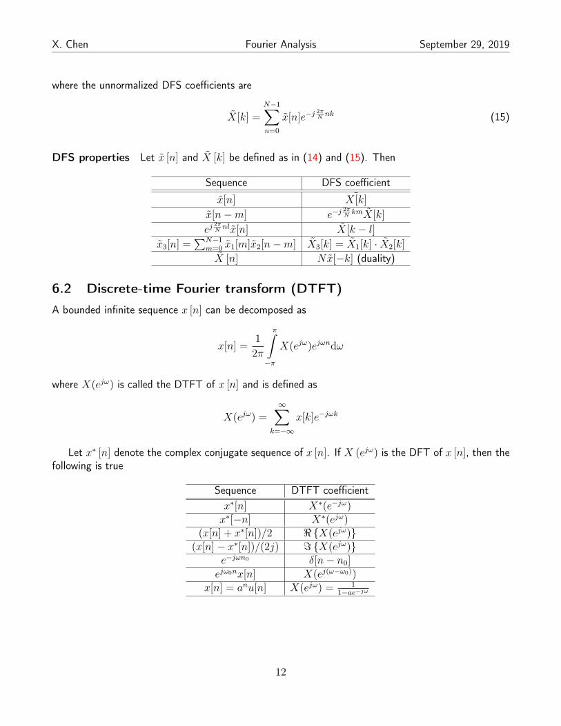
where the unnormalized DFS coefficients are

X̃[k] =N−1∑n=0

x̃[n]e−j2πNnk (15)

DFS properties Let x̃ [n] and X̃ [k] be defined as in (14) and (15). Then

Sequence DFS coefficient

x̃[n] ˜X[k]

x̃[n−m] e−j2πNkmX̃[k]

ej2πNnlx̃[n] X̃[k − l]

x̃3[n] =∑N−1

m=0 x̃1[m]x̃2[n−m] X̃3[k] = X̃1[k] · X̃2[k]

X̃ [n] Nx̃[−k] (duality)

6.2 Discrete-time Fourier transform (DTFT)

A bounded infinite sequence x [n] can be decomposed as

x[n] =1

2π

π∫−π

X(ejω)ejωndω

where X(ejω) is called the DTFT of x [n] and is defined as

X(ejω) =∞∑

k=−∞

x[k]e−jωk

Let x∗ [n] denote the complex conjugate sequence of x [n]. If X (ejω) is the DFT of x [n], then thefollowing is true

Sequence DTFT coefficientx∗[n] X∗(e−jω)x∗[−n] X∗(ejω)

(x[n] + x∗[n])/2 <{X(ejω)}(x[n]− x∗[n])/(2j) ={X(ejω)}

e−jωn0 δ[n− n0]

ejω0nx[n] X(ej(ω−ω0))x[n] = anu[n] X(ejω) = 1

1−ae−jω

12


6.3 Discrete Fourier transform (DFT)

A bounded sequence x [n] defined on n ∈ {0, . . . , N − 1} can be decomposed as

x[n] =

1N

N−1∑k=0

X[k]ej2πNkn , n ∈ {0, . . . , N − 1}

0 , n /∈ {0, . . . , N − 1}

where X[k] is the DFT of x [n] and is defined as

X[k] =

N−1∑n=0

x[n]e−2πjNkn , k ∈ {0, . . . , N − 1}

0 , k /∈ {0, . . . , N − 1}

DFT properties

• the DFT pair x[n] ←→ X[k] (finite-length x [n]) is analogous to the DFS pair x̃[n] ←→ X̃[k](infinite-length periodic x̃ [n])

• if x[n] is real, then X(k) = X∗[N − k]

• if N ≥ L, then DFT are samples of DTFT

• let x1 [n]N©x2 [n] :=N−1∑m=0

x1[m]x2[(n−m) mod N ]. Then x1 [n]N©x2[n]←→ X1[k]X2[k]

• if x[n] = x[((−n))N ] = x[N − n], then X[k] is real

• DFT coefficient table:

Sequence DFT coefficientx[n] X[k]x∗[n] X∗[((−k))N ]

x∗[((−n))N ] X∗[k]

x[n]ej2πn`/N X[(k − `) mod N ]

x[((n− `))N ] X[k]e−j2πk`/N

<(x[n]) 12{X[((k))N ] +X∗[((−k))N ]}

=(x[n]) 12{X[((k))N ]−X∗[((−k))N ]}

12{x[n] + x∗[((−n))N ]} <(X[k])

12{x[n]− x∗[((−n))N ]} j=(X[k])

12{x[n] + x[−n]}

∑N−1n=0 x[n] cos( 2πkn

2N−1)

x[n] ∈ R X[k] = X∗[N − k]

Reference

[EK]: ERwin Kreyszig, Advanced Engineering Mathematics, 10th edition[AO]: Alan Oppenheim et al., Discrete-time Signal Processing, 2nd edition

13

lecture notes fourier analysis - university of washington

Documents