lecture notes in computer science 6358
TRANSCRIPT

Lecture Notes in Computer Science 6358Commenced Publication in 1973Founding and Former Series Editors:Gerhard Goos, Juris Hartmanis, and Jan van Leeuwen
Editorial Board
David HutchisonLancaster University, UK
Takeo KanadeCarnegie Mellon University, Pittsburgh, PA, USA
Josef KittlerUniversity of Surrey, Guildford, UK
Jon M. KleinbergCornell University, Ithaca, NY, USA
Alfred KobsaUniversity of California, Irvine, CA, USA
Friedemann MatternETH Zurich, Switzerland
John C. MitchellStanford University, CA, USA
Moni NaorWeizmann Institute of Science, Rehovot, Israel
Oscar NierstraszUniversity of Bern, Switzerland
C. Pandu RanganIndian Institute of Technology, Madras, India
Bernhard SteffenTU Dortmund University, Germany
Madhu SudanMicrosoft Research, Cambridge, MA, USA
Demetri TerzopoulosUniversity of California, Los Angeles, CA, USA
Doug TygarUniversity of California, Berkeley, CA, USA
Gerhard WeikumMax Planck Institute for Informatics, Saarbruecken, Germany
Willem Jonker Milan Petkovic (Eds.)
SecureData Management
7th VLDB Workshop, SDM 2010Singapore, September 17, 2010Proceedings
13

Volume Editors
Willem JonkerPhilips Research EuropeHigh Tech Campus 34, 5656 AE Eindhoven, The NetherlandsE-mail: [email protected] of TwenteDepartment of Computer ScienceEnschede, The NetherlandsE-mail: [email protected]
Milan PetkovicPhilips Research EuropeHigh Tech Campus 34, 5656 AE Eindhoven, The NetherlandsE-mail: [email protected] University of TechnologyFaculty of Mathematics and Computer Science (HG 9.85)Eindhoven, The NetherlandsE-mail: [email protected]
Library of Congress Control Number: 2010933962
CR Subject Classification (1998): K.6.5, D.4.6, E.3, C.2, H.4, H.3
LNCS Sublibrary: SL 3 – Information Systems and Application, incl. Internet/Weband HCI
ISSN 0302-9743ISBN-10 3-642-15545-6 Springer Berlin Heidelberg New YorkISBN-13 978-3-642-15545-1 Springer Berlin Heidelberg New York
This work is subject to copyright. All rights are reserved, whether the whole or part of the material isconcerned, specifically the rights of translation, reprinting, re-use of illustrations, recitation, broadcasting,reproduction on microfilms or in any other way, and storage in data banks. Duplication of this publicationor parts thereof is permitted only under the provisions of the German Copyright Law of September 9, 1965,in its current version, and permission for use must always be obtained from Springer. Violations are liableto prosecution under the German Copyright Law.
springer.com
© Springer-Verlag Berlin Heidelberg 2010Printed in Germany
Typesetting: Camera-ready by author, data conversion by Scientific Publishing Services, Chennai, IndiaPrinted on acid-free paper 06/3180

Preface
The VLDB Secure Data Management Workshop was held for the 7th timethis year.
The topic of data security remains an important area of research especiallydue to the growing proliferation of data in open environments as a result ofemerging data services such as cloud computing, location based services, andhealth-related services. Confidentiality is the main driving force behind the re-search that covers topics such as privacy enhancing technologies, access control,and search in encrypted data.
We received 20 submissions from which the program committee selected 10papers to be presented at the workshop and included in the proceedings (50%acceptance rate). In addition, we are proud that Elisa Bertino accepted our invi-tation to give a keynote for which she selected the topic of data trustworthiness.We hope the papers collected in this volume will stimulate your research inthis area.
The regular papers in the proceeding have been grouped into two sections.The first section focuses on privacy. The papers in this section present a balancedmix of theoretical work on anonymity and application-oriented work.
The second section focuses on data security in open environments. The papersaddress issues related to the management of confidential data that is stored inor released to open environments, such as, for example, in cloud computing.
We wish to thank all the authors of submitted papers for their high-qualitysubmissions. We would also like to thank the program committee members aswell as additional referees for doing an excellent review job. Finally, let us ac-knowledge the work of Luan Ibraimi, who helped in the technical preparation ofthe proceedings.
July 2010 Willem JonkerMilan Petkovic

Organization
Workshop Organizers
Willem Jonker Philips Research/University of Twente,The Netherlands
Milan Petkovic Philips Research/Eindhoven University ofTechnology, The Netherlands
Program Committee
Gerrit Bleumer Francotyp-Postalia, GermanyLjiljana Brankovic University of Newcastle, AustraliaSabrina De Capitanidi Vimercati University of Milan, ItalyErnesto Damiani University of Milan, ItalyEric Diehl Techicolor, FranceLee Dong Hoon Korea University, South KoreaJeroen Doumen Irdeto, The NetherlandsCsilla Farkas University of South Carolina, USAElena Ferrari University of Insubria, ItalySimone Fischer-Hubner Karlstad University, SwedenTyrone Grandison IBM Almaden Research Center, USADieter Gollmann Technische Universitat Hamburg-Harburg,
GermanyMarit Hansen Independent Centre for Privacy Protection,
GermanyMin-Shiang Hwang National Chung Hsing University, TaiwanMizuho Iwaihara Kyoto University, JapanSushil Jajodia George Mason University, USATon Kalker HP Labs, USAMarc Langheinrich Universita della Svizzera italiana (USI),
SwitzerlandNguyen Manh Tho Vienna University of Technology, AustriaNick Mankovich Philips Medical Systems, USASharad Mehrotra University of California at Irvine, USAStig Frode Mjølsnes Norwegian University of Science
and Technology, NorwayEiji Okamoto University of Tsukuba, JapanSylvia Osborn University of Western Ontario, CanadaGunther Pernul University of Regensburg, GermanyBirgit Pfitzmann IBM Watson Research Lab, Switzerland

VIII Organization
Bart Preneel K.U.Leuven, BelgiumKai Rannenberg Goethe University Frankfurt, GermanyAndreas Schaad SAP Labs, FranceNicholas Sheppard Queensland University of Technology, AustraliaJason Smith Queensland University of Technology, AustraliaMorton Swimmer John Jay College of Criminal Justice/CUNY,
USAClark Thomborson University of Auckland, New ZealandSheng Zhong State University of New York at Buffalo, USA
Additional Referees
Mamadou Diallo University of California at Irvine, USAChristian Kahl Goethe University Frankfurt, GermanyChristian Weber Goethe University Frankfurt, Germany

Table of Contents
Keynote Paper
Assuring Data Trustworthiness – Concepts and Research Challenges . . . . 1Elisa Bertino and Hyo-Sang Lim
Privacy Protection
On-the-Fly Hierarchies for Numerical Attributes in DataAnonymization . . . . . . . . . . . . . . . . . . . . . . . . . . . . . . . . . . . . . . . . . . . . . . . . . . 13
Alina Campan and Nicholas Cooper
eM2: An Efficient Member Migration Algorithm for Ensuringk-Anonymity and Mitigating Information Loss . . . . . . . . . . . . . . . . . . . . . . . 26
Phuong Huynh Van Quoc and Tran Khanh Dang
Constrained Anonymization of Production Data: A ConstraintSatisfaction Problem Approach . . . . . . . . . . . . . . . . . . . . . . . . . . . . . . . . . . . . 41
Ran Yahalom, Erez Shmueli, and Tomer Zrihen
Privacy Preserving Event Driven Integration for Interoperating Socialand Health Systems . . . . . . . . . . . . . . . . . . . . . . . . . . . . . . . . . . . . . . . . . . . . . . 54
Giampaolo Armellin, Dario Betti, Fabio Casati,Annamaria Chiasera, Gloria Martinez, and Jovan Stevovic
Data Security in Open Environments
Joining Privately on Outsourced Data . . . . . . . . . . . . . . . . . . . . . . . . . . . . . . 70Bogdan Carbunar and Radu Sion
Computationally Efficient Searchable Symmetric Encryption . . . . . . . . . . 87Peter van Liesdonk, Saeed Sedghi, Jeroen Doumen,Pieter Hartel, and Willem Jonker
Towards the Secure Modelling of OLAP Users’ Behaviour . . . . . . . . . . . . . 101Carlos Blanco, Eduardo Fernandez-Medina, Juan Trujillo, andJan Jurjens
A Formal P3P Semantics for Composite Services . . . . . . . . . . . . . . . . . . . . . 113Assadarat Khurat, Dieter Gollmann, and Joerg Abendroth

X Table of Contents
A Geometric Approach for Efficient Licenses Validation in DRM . . . . . . . 132Amit Sachan, Sabu Emmanuel, and Mohan S. Kankanhalli
Differentially Private Data Release through MultidimensionalPartitioning . . . . . . . . . . . . . . . . . . . . . . . . . . . . . . . . . . . . . . . . . . . . . . . . . . . . . 150
Yonghui Xiao, Li Xiong, and Chun Yuan
Author Index . . . . . . . . . . . . . . . . . . . . . . . . . . . . . . . . . . . . . . . . . . . . . . . . . . 169

Assuring Data Trustworthiness -
Concepts and Research Challenges�
Elisa Bertino and Hyo-Sang Lim
Department of Computer Science, Purdue University, USA{bertino,hslim}@cs.purdue.edu
Abstract. Today, more than ever, there is a critical need to share datawithin and across organizations so that analysts and decision makerscan analyze and mine the data, and make effective decisions. However,in order for analysts and decision makers to produce accurate analysisand make effective decisions and take actions, data must be trustwor-thy. Therefore, it is critical that data trustworthiness issues, which alsoinclude data quality, provenance and lineage, be investigated for organi-zational data sharing, situation assessment, multi-sensor data integrationand numerous other functions to support decision makers and analysts.The problem of providing trustworthy data to users is an inherentlydifficult problem that requires articulated solutions combining differentmethods and techniques. In the paper we first elaborate on the datatrustworthiness challenge and discuss a framework to address this chal-lenge. We then present an initial approach for assess the trustworthinessof streaming data and discuss open research directions.
Keywords: Data Trustworthiness, Data Integrity and Quality, Security,Policy.
1 Introduction
Today, more than ever, there is a critical need to share data among organiza-tions so that analysts and decision makers can analyze and mine the data, andmake effective decisions. Meanwhile, in many recent applications such as traf-fic monitoring systems and power grid management systems, a large amountof data that can convey important information for critical decision making iscollected from distributed sources. In order for analysts and decision makers toproduce accurate analysis, make effective decisions, and take actions, data mustbe trustworthy. Therefore, it is critical that data trustworthiness issues, whichalso include data quality and provenance, be investigated for organizational datasharing, situation assessment, multi-sensor data integration, and numerous otherfunctions to support decision makers and analysts. Without trustworthiness, the
� The authors have been partially supported by AFOSR grant FA9550-07-1-0041 “Sys-tematic Control and Management of Data Integrity, Quality and Provenance forCommand and Control Applications”.
W. Jonker and M. Petkovic (Eds.): SDM 2010, LNCS 6358, pp. 1–12, 2010.c© Springer-Verlag Berlin Heidelberg 2010

2 E. Bertino and H.-S. Lim
usefulness of data becomes diminished as any information extracted from themcannot be trusted with sufficient confidence.
It is thus important to provide a comprehensive solution for assessing andassuring the trustworthiness of the information collected in such data sharingsystems since decisions and analyses are largely affected by this information.Attacks or unexpected accidents may result in bad data being provided to criticalcomponents of the system. These components may in turn take wrong decisionsor generate inaccurate analyses that can result in damages to real-world objectssuch as manufacturing facilities or power plants. For example, in an electricpower grid which consists of 270 utilities using a SCADA (Supervisory Controland Data Acquisition) system that can contain up to 50,000 data collectionpoints and over 3,000 public/private electric utilities, any single point of failurecan disrupt the entire process flow and can potentially cause a domino effectthat shuts down the entire systems [11].
In general the problem of providing “good” data to users and applicationsis an inherently difficult problem which often depends on the application anddata semantics as well as on the current context and situation. In many cases,it is crucial to provide users and applications not only with the needed data,but with also an evaluation indicating how much the data can be trusted. Beingable to do so is particularly challenging especially when large amounts of dataare generated and continuously transmitted across the system. Also solutions forimproving the data, like those found in data quality, may be very expensive andmay require access to data sources which may have access restrictions, becauseof data sensitivity. Also even when one adopts methodologies to assure thatthe data is of good quality, errors may still be introduced and low quality databe used; therefore, it is important to assess the damage resulting from the useof such data, to track and contain the spread of errors, and to recover. Themany challenges of assuring data trustworthiness require articulated solutionscombining different approaches and techniques including data integrity, dataquality, and data provenance. In this paper we discuss some components of sucha solution and highlight relevant research challenges.
Our approach for assuring information trustworthiness is based on a compre-hensive framework composed of two key elements. The first element is repre-sented by trust scores that are to associated with all data items to indicate thetrustworthiness of each data item. Trust scores can be used for data comparisonor ranking. They can be also used together with other factors (e.g., informationabout contexts and situations, past data history) for deciding about the useof the data items. Our framework provides a trust score computation methodwhich is based on the concept of data provenance, as provenance gives impor-tant evidence about the origin of the data, that is, where and how the datais generated. The second element of our framework is the notion of confidencepolicy [8]. Such a policy specifies a range of trust scores that a data item, or setof data items, must have for use by the application or task. It is important tonotice that the required range of trust scores depends on the purpose for whichthe data have to be used. In our framework, confidence policies are integrated

Assuring Data Trustworthiness - Concepts and Research Challenges 3
with query processing in that query results are filtered by the policies before be-ing returned to the application. Our confidence policy language includes manyother components that can be used to formulate articulated conditions aboutdata usage.
We have applied our framework to sensor networks which are being increas-ingly deployed in a large variety of novel areas, like supervisory systems, e-health,and e-surveillance. In all those areas, it is crucial to assess the trustworthinessof sensed data in order to support correct decisions as sensors may be deployedin hostile environments and are usually connected via wireless networks whichcan be an easy target for adversaries. In this application, with respect to the as-sessment of trust scores, we exploits an interdependency property between dataitems and sensors, i.e., the trust score of the data affects the trust score of thesensors that created and manipulated the data, and vice-versa. To reflect theinterdependency, we have proposed a cyclic method that generates: (1) trustscores of data items from those of sensors and (2) trust scores of sensors fromthose of data items whenever new data items arrive.
The rest of the paper is organized as follows. Section 2 discusses related work.Section 3 describes our framework for assuring information trustworthiness. Sec-tion 4 describes the application of our framework to sensor network environ-ments. Section 5 discusses open research issues and directions related to ourframework. We finally summarize and conclude the paper in Section 6.
2 Related Work
Currently there is no comprehensive approach to the problem of high assurancedata trustworthiness. However, our approach is related to several areas includingdata integrity, data quality, and data provenance.
Data Integrity. Biba [4] was the first to address the issue of integrity in in-formation systems. He proposed an approach based on a hierarchical lattice ofintegrity levels so as to ensure integrity by blocking the flow of information fromlow-integrity objects to high-integrity subjects. However, Biba’s approach is noteasy to use because it is not clear how to determine the appropriate integritylevels as there are no criteria for determining them. Clark and Wilson [6] pro-posed another model for data integrity in commercial environments. The modelconsists of two key notions: well-formed transactions and separation of duty. Awell-formed transaction is one that only manipulates data in trusted ways so topreserve the consistency of data. Separation of duty mandates separating all op-erations into several subparts and executing each subpart by a different subject.However, the model has some limitations in that it categorizes data integrityonly according to two levels: valid and invalid. Our approach is more compre-hensive than those models in that it provides mechanisms driven by confidencepolicies and provides an approach to determine the data trust level based ondata provenance information.
Data quality. Ranging fromdatawarehousing to supply chainmanagement, dataquality is a serious concern for professionals involved in a wide array of information

4 E. Bertino and H.-S. Lim
systems. One industry study estimated the total cost to the US economy of dataquality problems at over US$600 billion per annum [10]. Data quality has been in-vestigated from different perspectives, depending on the precise meaning assignedto the notion of data quality. Data are of high quality “if they are fit for their in-tended uses in operations, decision making and planning” [16]. Alternatively, thedata are deemed of high quality if they correctly represent the real-world constructto which they refer. A number of theoretical frameworks consider data quality. Aframework is based on semiotics to evaluate the quality of the form, meaning anduse of the data [22]. Another theoretical approach analyzes the ontological natureof information systems to define data quality rigorously [26]. Tools have also beendeveloped for analyzing and repairing poor quality data, through the use, for ex-ample, of record linkage techniques.
Data provenance. Data provenance, also referred to as lineage or pedigree,has been widely investigated. Approaches have been developed for tracking theprovenance of the query results, i.e., recording the sequence of steps taken in aworkflow system to derive the dataset, and computing confidence levels of thequery results [1,2,12,23]. For example, Widom et al. [27] developed the Trio sys-tem which supports management of information about data accuracy and lineage(provenance). Sarma et al. [24] developed an approach to compute lineage andconfidence in probabilistic databases according to a decoupled strategy. Theseapproaches compute the confidence of query results based on the confidence onthe base tuples in the database, i.e., they assume that the confidence of each basetuple (i.e., data item) is known, whereas we actually compute the trust score foreach data item. Vijayakumar and Plale [25] propose a system architecture fornear-real time provenance collection in data streams. They focus on identifyinginformation which represents provenance of a data item from real time datastreams, capturing provenance history of streams, tracing the source of a streamlong after the process has completed. Data provenance in data streaming has alsobeen investigated in IBM’s Century [5,20], which is a biomedical data streamsystem for online healthcare analytics.
3 A Framework for Assuring Information Trustworthiness
Figure 1 shows an overview of our framework for assuring information trustwor-thiness. The figure illustrates how data are managed, processed, and deliveredto users. As shown in the figure, the proposed framework consists of three majorcomponents: trustworthiness assessment, query and policy evaluation, and dataquality management. The role of each component is as follows:
Trustworthiness assessment associates trust scores with data in the database.A trust score is a numeric value ranging from 0 to 1 where 0 means the lowesttrustworthiness and 1 means the highest trustworthiness. Such a trust score is akey notion of our framework since it indicates trustworthiness of the data itemand can be used for data comparison or ranking. Trust scores can be obtained byusing various factors such as the trustworthiness of data providers and the wayin which the data has been collected. In our framework, we especially focus on

Assuring Data Trustworthiness - Concepts and Research Challenges 5
data provenance for computing trust scores. This idea is based on the principlethat the more trustworthy data a source provides, the more trusted the sourceis considered. There is thus an interdependency property between data providersand data items with respect to the assessment of their trust scores, i.e., thetrust score of the data affects the trust score of the data providers that createdand manipulated the data, and vice-versa. To reflect such interdependency inassessing trustworthiness, we maintain trust scores for both data items and dataproviders. That is, the trustworthiness assessment component computes (1) trustscores of data items based on those of data providers and (2) trust scores of dataproviders based on those of data items.
Query and policy evaluation executes user queries, each of which has its ownconfidence policy [3,8]. Confidence policies specify confidence range [qmax, qmin]that query results must have for use by the application or task. Such a confidencepolicy is a key notion of our framework since it restricts access to the query resultsbased on the trust score of the query results and application’s requirements. Werefer to queries enforcing such policies as confidence policy-compliant queries. Foreach user query Q with its confidence policy [qmax, qmin], the query and policyevaluation component first obtains the resulting data items by evaluating thegiven query Q, and then, returns data items of which trust scores are in betweenqmax and qmin.
Data quality management tries to control data quality manually or automat-ically. Since some query results will be filtered out by the confidence policy, auser may not receive enough data to make a decision. To prevent such a lackof information in applications, we need to provide a method to dynamically in-crement the data trust scores. The method includes collecting additional data,changing data delivery paths, and cross-checking the data with other informa-tion. The component should consider the cost for improving data quality whendetermining which data should be selected and how much the trust score shouldbe increased to satisfy the confidence range stated by the confidence policies.
DatabaseQuery Evaluation
Policy Evaluation
Data Quality Management
Trustworthiness Assessment queries with confidence policies
data items with trust scores
[ ]( )min max, ,Q q q
( ),d
d s
Fig. 1. An overall framework for assuring information trustworthiness
Our framework has many advantages in assuring information trustworthiness.First, it provides a measure for trustworthiness of data (i.e., trust scores) and an

6 E. Bertino and H.-S. Lim
approach to determine those values. Second, it provides policies by using whichone can specify which the confidence is required for use of certain data in certaintasks. With such policies, our solution supports fine-grained integrity tailored tospecific data and tasks. Third, it provides an approach to dynamically adjustthe data trustworthiness so to provide users with query replies that comply withthe confidence policies.
4 An Application to Sensor Networks
In this section, we discuss the application of our framework to sensor networks.
4.1 Adopting the Framework into Sensor Networks
In sensor networks, it is extremely important to assess data quality since sensorscan be deployed in hostile environments and the wireless networks connectingthem can be easily attacked. Therefore, it is crucial to assess the quality ofsensed data and increase the quality whenever possible, in order to support cor-rect decisions in sensor network applications. Additionally, in sensor networkenvironments, 1) data items arrive incrementally and 2) trustworthiness of sen-sors and their readings can dynamically change as time goes on. Figure 2 showshow our framework is adopted for such dynamic sensor networks.
In the framework, the trustworthiness assessment component obtains trustscores of data items based on those of network nodes and (periodically) up-dates the trust scores to reflect the effect of the newly arrived data items. Italso maintains and updates trust scores of network nodes based on the scoresof data items. Query and policy evaluation components continuously executequeries (each of which has its own confidence policy) whenever a new data itemarrives from sensors. The data quality management component improves trust-worthiness by adjusting data rates, increasing/decreasing the number of sensornodes, or changing delivery paths. Obviously, data quality affects trust scores,and many approaches [7,14,21] in the sensor networks area have addressed theissue of controlling data quality. In this section, we focus on trustworthinessassessment so as to get reasonable trust scores for sensor readings.
1
query & policy evaluation
trust score computation
(focus of the paper)
sensor network
data quality management
stream of data items(with provenance)
change of data quality
queries with confidence ranges
data items with trust scores
DSMS
stream of data items (with trust scores)
evaluation results
[ ]( )min max, ,Q q q
( ), dd s
trust scores ofnetwork nodes
Fig. 2. Adopting our framework into sensor networks

Assuring Data Trustworthiness - Concepts and Research Challenges 7
4.2 Modeling Sensor Networks and Data Provenances
Before describing the computation of trust scores, we explain data provenancewhich is an important information for assessing trustworthiness in our approach.We model the sensor network as a graph of G(N, E) where N is a set of nodes(i.e., sensors) and E is a set of network connections between nodes. We assumethat the sensors are in ad-hoc networks which send data items to DSMSs byrelaying because of the insufficient data transmission bandwidth. In this kind ofnetwork, the sensors are categorized into three types according to their roles: 1)terminal nodes that generate data items and send them to one or more inter-mediate or server nodes; 2) intermediate nodes that receive data items from oneor more terminal or intermediate nodes, and pass them to other intermediate orserver nodes; they may also generate an aggregated data item from the receiveddata items and send the aggregated item to other intermediate or server nodes;3) server nodes that receive data items and evaluate continuous queries basedon those items.
We introduce two types of data provenance: the physical provenance and thelogical provenance. The physical provenance of a data item indicates where theitem was produced and how it was delivered to the server. We exploit the physicalprovenance to compute trust scores. The physical provenance can be representedas a path from a terminal node to a server node or a tree if there are more thantwo terminal nodes involved in the generation of the data item. The logicalprovenance of a data item represents the semantic meaning of the data item inthe context of a given application. For example, the logical provenance can bea chain of employees who used the data item, or a trail of business logics thatprocessed the data item. The logical provenance is used for grouping data itemsinto semantic events with the same meaning or purpose.
4.3 Computing Trust Scores
To obtain trust scores, we propose a cyclic framework based on the interdepen-dency property [3,8] between data items and their related network nodes. Thatis, the trust scores of data items affect the trust scores of network nodes, andsimilarly the trust scores of network nodes affect those of data items. In addition,the trust scores need to be continuously evolved in the stream environment sincenew data items continuously arrive to the server. Thus, a cyclic framework isadequate to reflect these interdependency and continuous evolution properties.Figure 3 shows the cyclic framework according to which the trust score of dataitems and the trust score of network nodes are continuously updated. The trustscores are computed for the data items of the same event (identified by logicalprovenance) in a given streaming window.
As shown in Figure 3, we maintain three different types of trust scores, thatis, current, intermediate, and next trust scores, to reflect the interdependencyand continuous evolution properties in computing trust scores. We note that,since new data items are continuously added to the stream, executing the cycleonce whenever a new data item arrives is enough to reflect the interdependencyand continuous evolution properties in the stream environment.

8 E. Bertino and H.-S. Lim
Current trust scores
of nodes ( )
Next trust scores
of nodes ( )
Intermediate trust
scores of nodes ( )
+
Current trust scores
of data items ( )
Intermediate trust
scores of data items ( )
Next trust scores
of data items ( )
A set of data items of
the same event
in a current window
+
1
2
3
5
4
6
ns
ns)
ns
ds
ds)
ds
Fig. 3. The cyclic framework for computing the trust scores of data items and networknodes
Our framework works as follows. Trust scores are initially computed basedon the values and provenance of data items; we refer to these trust scores asimplicit trust scores. To obtain these trust scores, we use two types of similarityfunctions: value similarity inferred from data values, and provenance similarityinferred from physical provenances. Value similarity is based on the principlethat the more data items referring to the same real-world event have similar val-ues, the higher the trust scores of these items are. We observe that most sensordata referring to the same event follow the normal distribution, and propose asystematic approach for computing trust scores based on value similarity un-der the normal distribution. Provenance similarity is based on the observationthat different physical provenances of similar data values may increase the trust-worthiness of data items. In other words, different physical provenances providemore independent data items. For more details, please refer to our technicalreport [18].
5 Research Issues and Challenges
In this section, we discuss open research directions for each component of ourframework described in Section 3.
Trustworthiness Assessment
– Data/provenance similarity measures. Measuring data similarity is essentialin our trust score computation. If we only handle numeric values, the simi-larity can be easily measured with the difference or Euclidian distance of thevalues. However, if the value is non-numeric (such as text data), we need toinclude modeling techniques able to take into account data semantics. Forexample, if data are names of places, we need to consider spatial relation-ships in the domain of interest. Possible approaches that can be used includesemantic web techniques, like ontologies and description logics. Similarly,measuring provenance similarity is not easy especially when the provenanceis complex. The edit distance which uses the minimum amount of distor-tion that is needed to transform one graph into another is the most popularsimilarity measure in graph theory. However, computing the edit distance

Assuring Data Trustworthiness - Concepts and Research Challenges 9
for general graphs is known to be an NP-hard problem [13]. Therefore, weneed an approximate similarity measure method which efficiently comparesgraph-shape provenances.
– Correlation among data sources. The relationships among the various datasources could be used to create more detailed models for assigning trust toeach data source. For example, if we do not have good prior informationabout the trustworthiness of a particular data source, we may try to use dis-tributed trust computation approaches such as EigenTrust [17] to compute atrust value for the data source based on the trust relationships among datasources. In addition, even if we observe that the same data is provided bytwo different sources, if these two sources have a very strong relationship,then it may not be realistic to assume that the data is provided by two in-dependent sources. An approach to address such issue is to develop “sourcecorrelation” metrics based on the strength of the relationship among possibledata sources. Finally, in some cases, we may need to know “how importantis a data sources within our information propagation network?” to reasonabout possible data conflicts. To address such issue one can apply varioussocial network centrality measures such as degree, betweenness, closeness,and information centralities [15] to assign importance values to the variousdata sources.
– Secure data provenance. Since data provenance is a key evidence for measur-ing the trustworthiness of data items, it should be protected from tamperingwhen flowing across the various parties. For example, if the provenance ofan untrustworthy data item is modified to a trustworthy node, the quality ofthe data item is assessed as high, even though in reality the data item has alow quality. Conventional digital signature or cryptography techniques canbe used to prevent such malicious attacks. Another approach can be basedon techniques for controlled and cooperative updates of XML documents inByzantine and failure-prone distributed systems [19]. One could develop anXML language for encoding provenance information and use such techniquesto secure provenance documents. We also should consider reducing the over-head of these techniques since it directly affects to the performance of datacollection and query processing.
Query and Policy Evaluation
– Expressive power of confidence policies. We need to improve the expressivityof the confidence policy model since the current policy language is verysimple. It should be possible to support a more fine-grained specification ofconfidence requirements concerning data use whereby for a given task androle, one can specify different trust scores for different categories of data.The model should support the specification of subjects, in terms of subjectattributes and profiles other than the subject role. If needed, exceptions tothe policies should be supported; a possible approach is to support strongpolicies, admitting no exceptions, and weak policies, admitting exceptions.If exceptions are allowed for a policy (set of policies), the policy enforcement

10 E. Bertino and H.-S. Lim
mechanism should support the gathering of evidence about the need forexceptions. Such evidence is crucial in order to refine confidence policies.
– Policy provisioning. An important issue is related to the confidence policyprovisioning. Provisioning refers to assigning confidence policies to specifictasks, users, and data and, because it very much depends from the applica-tions and data semantics, it may be quite difficult. To address such issue,one approach is the use of machine learning techniques.
– Performance. Efficient evaluation of confidence policies is crucial to achievehigh performance of responding user query requests. Especially, in sensornetwork environment, it becomes more important due to fast input rates andreal-time processing requirement. One possible solution is tightly combiningquery processing and policy evaluation so as to retrieve data items whichsatisfy both query conditions and trust score ranges at once.
Data Trustworthiness Improvement
– Efficiently improve data trustworthiness. We use data provenance for notonly measuring but also improving data trustworthiness. As we discussed inSection 3, the data quality management component tries to improve datatrustworthiness when the number of results satisfying a confidence policy istoo small. Many methods can be adopted to improve trustworthiness: frommanually checking data items by hand to automatically comparing dataitems with other information. The cost of each method depends on the op-timization criteria adopted, like time and financial cost. Therefore, suitablecost models need to be developed. Also, trustworthiness improvement algo-rithms need to be devised for determining suitable data items for which theincrease in the trust scores can lead to the minimum cost. Because it is likelythat finding the optimal solution may be computationally very expensive,heuristics need to be devised.
6 Concluding Remarks
In this paper, we have discussed a comprehensive framework for assuring infor-mation trustworthiness, based on two novel concepts: trust scores and confidencepolicies. Our framework is very general and can be used in different applica-tion domains. In the paper we have discussed the application to the problemof assessing the trustworthiness of data streaming in sensor network. Anotherapplication has been developed for assessing the trustworthiness of locations ofindividuals [9]. Our work has many open research directions, which we have alsodiscussed in the paper. In addition to these directions, developing new applica-tions is an important step for future work.
References
1. Abiteboul, S., Kanellakis, P., Grahne, G.: On the Representation and Querying ofSets of Possible Words. SIGMOD Record 16(3), 34–48 (1987)
2. Barbara, D., Garcia-Molina, H., Porter, D.: The Management of Probabilistic Data.IEEE Trans. on Knowledge and Data Engineering 4(5), 487–502 (1992)

Assuring Data Trustworthiness - Concepts and Research Challenges 11
3. Bertino, E., Dai, C., Lim, H.-S., Lin, D.: High-Assurance Integrity Techniques forDatabases. In: Proc. of the 25th British Nat’l Conf. on Databases, Cardiff, UK,pp. 244–256 (July 2008)
4. Biba, K.J.: Integrity Considerations for Secure Computer Systems. Technical Re-port TR-3153, Mitre (1977)
5. Blount, M., et al.: Century: Automated Aspects of Patient Care. In: Proc. 13thIEEE Int’l. Conf. on Embedded and Real-Time Computing Systems and Applica-tions (RTCSA 2007), Daegu, Korea, pp. 504–509 (August 2007)
6. Clark, D., Wilson, D.: A Comparison of Commercial and Military computer Secu-rity Policies. In: Proc. of IEEE Symposium on Security and Privacy (1987)
7. David, Y., Erich, N., Jim, K., Prashant, S.: Data Quality and Query Cost in Wire-less Sensor Networks. In: Proc. of the 5th IEEE Int’l Conf. on Pervasive Comput-ing and Communications Workshops, White Plains, New York, USA, pp. 272–278(March 2007)
8. Dai, C., et al.: Query Processing Techniques for Compliance with Data ConfidencePolicies. In: Proc. of the 6th VLDB Workshop on Secure Data Management, Lyon,France, pp. 49–67 (2009)
9. Dai, C., Lim, H.-S., Bertino, E., Moon, Y.-S.: Assessing the Trustworthiness ofLocation Data Based on Provenance. In: Proc. of the 17th ACM SIGSPATIALInt’l Symposium on Advances in Geographic Information Systems, Seattle, USA,pp. 276–285 (November 2009)
10. Eckerson, W.: Data Warehousing Special Report: Data quality and the bottomline, http://www.adtmag.com/article.aspx?id=6321
11. Fernandez, J., Fernandez, A.: SCADA systems: vulnerabilities and remediation.Journal of Computing Sciences in Colleges 20(4), 160–168 (2005)
12. Fuhr, N.: A Probabilistic Framework for Vague Queries and Imprecise Informationin Databases. In: Proc. of the 16th Int’l. Conf. on Very Large Data Bases, Brisbane,Australia, pp. 696–707 (August 1997)
13. Garey, M.R., Johnson, D.S.: Computers and Intractability, A Guide to the Theoryof NP-Completeness (1990)
14. Hwang, S.-Y., Liu, P.-Y., Lee, C.-H.: Using Resampling for Optimizing ContinuousQueries in Wireless Sensor Networks. In: Proc. of the 8th Int’l. Conf. on IntelligentSystems Design and Applications, Kaohsiung, Taiwan, pp. 107–110 (November2008)
15. Jackson, M.O.: Social and Economics Networks. Princeton University Press,Princeton (2008)
16. Juran, J.M.: Juran on Leadership for Quality - an Executive Handbook. Free Press(1989)
17. Kamvar, S.D., Schlosser, M.T., Garcia-Molina, H.: The EigenTrust Algorithm forReputation Management in P2P Networks. In: Proc. of Twelfth Int’l. World WideWeb Conf., New York, USA, pp. 640–651 (2003)
18. Lim, H.-S., Moon, Y.-S., Bertino, E.: Assessing the Trustworthiness of StreamingData. Technical Report TR 2010-09, CERIAS (2010)
19. Mella, G., Ferrari, E., Bertino, E., Koglin, Y.: Controlled and Cooperative Updatesof XML Documents in Byzantine and Failure-prone Distributed Systems. ACMTransactions on Information and System Security 9, 421–460 (2006)
20. Misra, A., Blount, M., Kementsietsidis, A., Sow, D.M., Wang, M.: Advances andChallenges for Scalable Provenance in Stream Processing Systems. In: Freire, J.,Koop, D., Moreau, L. (eds.) IPAW 2008. LNCS, vol. 5272, pp. 253–265. Springer,Heidelberg (2008)

12 E. Bertino and H.-S. Lim
21. Olston, C., Jiang, J., Widom, J.: Adaptive Filters for Continuous Queries overDistributed Data Streams. In: Proc. Int’l. Conf. on Management of Data, pp. 563–574. ACM SIGMOD, San Diego (June 2003)
22. Price, R., Shanks, G.: A Semiotic Information Quality Framework. In: Proc. IFIPInternational Conference on Decision Support Systems (DSS 2004), Prato, Italy(2004)
23. Sarma, A.D., Benjelloun, O., Halevy, A., Widom, J.: Working Models for UncertainData. In: Proc. of the 22nd Int’l. Conf. on Data Engineering, Atlanta, USA, p. 7(April 2006)
24. Sarma, A.D., Theobald, M., Widom, J.: Exploiting Lineage for Confidence Compu-tation in Uncertain and Probabilistic Databases. In: Proc. of the 24th Int’l. Conf.on Data Engineering, Cancun, Mexico, pp. 1023–1032 (April 2008)
25. Vijayakumar, N., Plale, B.: Towards Low Overhead Provenance Tracking in NearReal-Time Stream Filtering. In: Moreau, L., Foster, I. (eds.) IPAW 2006. LNCS,vol. 4145, pp. 46–54. Springer, Heidelberg (2006)
26. Wand, Y., Wang, R.: Anchoring Data Quality Dimensions in Ontological Founda-tions. Communications of the ACM 39(11), 86–95 (1996)
27. Widom, J.: Trio: A System for Integrated Management of Data, Accuracy, andLineage. In: Proc. of the 2nd Biennial Conf. on Innovative Data Systems Research,Asilomar, USA, pp. 262–276 (January 2005)

W. Jonker and M. Petković (Eds.): SDM 2010, LNCS 6358, pp. 13–25, 2010. © Springer-Verlag Berlin Heidelberg 2010
On-the-Fly Hierarchies for Numerical Attributes in Data Anonymization
Alina Campan and Nicholas Cooper
Department of Computer Science, Northern Kentucky University, Highland Heights, KY 41099, USA
[email protected], [email protected]
Abstract. We present in this paper a method for dynamically creating hierarchies for quasi-identifier numerical attributes. The resulting hierarchies can be used for generalization in microdata k-anonymization, or for allowing users to define generalization boundaries for constrained k-anonymity. The construction of a new numerical hierarchy for a numerical attribute is performed as a hierarchical agglomerative clustering of that attribute’s values in the dataset to anonymize. Therefore, the resulting tree hierarchy reflects well the closeness and clustering tendency of the attribute’s values in the dataset. Due to this characteristic of the hierarchies created on-the-fly for quasi-identifier numerical attributes, the quality of the microdata anonymized through generalization based on these hierarchies is well preserved, and the information loss in the anonymization process remains in reasonable bounds, as proved experimentally.
Keywords: data privacy, k-anonymity, hierarchies for quasi-identifier numerical attributes.
1 Introduction
Attribute generalization is a disclosure control technique intensively used in data anonymization methods, together with data suppression. Generalization of quasi-identifier attributes is, for example, applied to mask initial microdata (a dataset where each tuple corresponds to one individual entity) to make it conform to k-anonymity-like models: k-anonymity [1], [2], l-diversity [3], p-sensitive k-anonymity [4], (α, k)-anonymity [5], t-closeness [6], (ε, m)-anonymity [7], l+-diversity [8], (τ, λ)-uniqueness [9] etc. The resulting data will present the k-anonymity property, which means that each tuple in the masked set will be identical with respect to the quasi-identifier attributes to at least k-1 other tuples in the set; also, depending on the anonymity model used, the masked data will also exhibit other statistical properties.
Generalization of a quasi-identifier attribute consists in replacing the actual value of the attribute with a less specific, more general value that is faithful to the original [10]. Initially, this technique was used for categorical attributes and employed predefined (static) domain and value generalization hierarchies [10]. Generalization was extended for numerical attributes either by using predefined hierarchies [11] or a

14 A. Campan and N. Cooper
hierarchy-free model [12]. The important distinction between using predefined hierarchies and performing a hierarchy-free generalization is as follows. Predefined hierarchies are constructed, normally manually by users, before the data masking process begins, and these hierarchies are used as they are, unchanged, for generalization. The hierarchy-free generalization inherently leads to the construction of a hierarchy during the anonymization process; the creation of such a hierarchy is usually guided by local optimum decisions taken during anonymization.
Another important aspect is how hierarchies are used for generalization. For a categorical attribute, generalization is based on a domain generalization hierarchy associated to that attribute. The values from different domains/levels of this hierarchy are represented in a tree called a value generalization hierarchy. Fig. 1 shows two examples of domain and value generalization hierarchies for attributes zip_code and gender of a microdata set containing personal information for individuals.
Fig. 1. Examples of domain and value generalization hierarchies
Generalization of categorical attributes, based on domain and value generalization hierarchies, comes in several flavors.
Generalization that maps all values of a quasi-identifier categorical attribute in the microdata set to a more general domain in its domain generalization hierarchy is called full-domain generalization [1], [12]. For example, a full-domain generalization for zip_code can consist in replacing all initial zip codes in the microdata with their corresponding ancestors located on the middle level in the value generalization hierarchy in Fig. 1: 48201 with 482**, 41075, 41076, 41088, and 41099 with 410**.
Generalization can also map an attribute’s values to different domains in its domain generalization hierarchy, each value being replaced by the same generalized value in the entire dataset [11]. This type of generalization was introduced by Iyengar in [11]. In this type of generalization, 48201 would be replaced with one and only one of its ancestors, for example 482**, in the entire dataset, while another one of the original values, let’s say 41075, could be replaced with its ***** ancestor across the entire dataset; note that the replacement, more general values, 482** and *****, are located on different levels in zip_code’s value generalization hierarchy.
Finally, the least restrictive generalization, called cell level generalization [13], extends Iyengar’s model [11] by allowing the same value to be mapped to different
G0 = {male, female}
G1 = {*} *
male female
Z1 = {482**, 410**}
Z2 = {*****}
Z0 = {48201, 41075, 41076, 41088, 41099}
*****
482** 410**
48201 41075 41076 41088 41099

On-the-Fly Hierarchies for Numerical Attributes in Data Anonymization 15
Tuples age zip_code gender Tuples age zip_code gender
r1 25 41076 Male r1 20-30 ***** Male
r2 25 41075 Male r2 20-30 ***** Male
r3 35 41099 Female r3 30-40 ***** Female
r4 38 48201 Female r4 30-40 ***** Female
r5 36 41075 Female r5 30-40 ***** Female
Initial non-generalized microdata set, zip_code and gender are categorical attributes with the hierarchies defined in Fig. 1.
Masked (i.e. anonymized) microdata set, k=2, full-domain generalization.
Tuples age zip_code gender Tuples age zip_code gender
r1 20-40 410** * r1 20-30 410** Male
r2 20-40 410** * r2 20-30 410** Male
r3 20-40 ***** * r3 30-40 ***** Female
r4 20-40 ***** * r4 30-40 ***** Female
r5 20-40 410** * r5 30-40 ***** Female
Masked microdata set, k=2, Iyengar generalization.
Masked microdata set, k=2, cell-level generalization.
Fig. 2. Examples of different types of generalizations
generalized values, in distinct tuples. Therefore, if cell level generalization is used, the same original zip code value 48201 could be replaced in different tuples with different ancestors: in our case, either 482** or *****.
We illustrate in Fig. 2 the differences between the above-mentioned types of generalization.
Generalization of numerical attributes using predefined hierarchies is similar to the generalization for categorical attributes.
The hierarchy-free generalization of numerical attributes replaces the set of values to be generalized to the smallest interval that includes all the initial values. For instance, the values: 35, 38, 36 for the attribute age are generalized to the interval [35-38]; again, the decision to replace these values with the mentioned interval is taken during the anonymization process and might apply only to a subset of the tuples in the microdata set. Other occurrences of the original values (35, 38, and 36) may be replaced with other values/intervals in other tuples in the microdata set. Note that overlapping of the intervals formed during generalization is possible.
While creating and using generalization hierarchies for categorical attributes is expected to be easy and natural enough for users of anonymization methods, constructing and employing predefined hierarchies for numerical attributes is not as straightforward. Usually, creating and understanding a hierarchy for categorical attributes is easier than for numerical attributes: the values of the categorical attribute are well established, discrete, have a natural hierarchical organization, while numerical attributes might have more diverse values, maybe are continuous, and

16 A. Campan and N. Cooper
rarely have a natural hierarchical structure. However, employing a “good” hierarchy in the anonymization process significantly impacts the quality of the masked data; depending on how well the hierarchy fits the distribution and grouping of the attribute’s values in the microdata set, the masked data can lose more or less from the information it inherently contains.
Hierarchy-free generalization for numerical attributes is a more flexible disclosure control technique, and helps to minimize the information loss that occurs in the masking process. It presents, however, an important down come: certain data anonymity models, such as constrained k-anonymity (which relies on boundaries imposed on the amount of generalization allowed in the anonymization process) require pre-existing hierarchies for numerical attributes [14].
We propose in this paper a new method for creating hierarchies for numerical attributes, based on its values in the dataset to be anonymized. The resulting hierarchy reflects the attribute’s values distribution and grouping (clustering), such that to support a reasonable information loss when used in anonymization.
The paper is structured as follows. The next section introduces our method for dynamically creating hierarchies for quasi-identifier numerical attributes. Section 3 explains how numerical hierarchies are used in k-anonymization and introduces information loss – a metric frequently employed in the data privacy domain for assessing the masked microdata quality, and which can be used both to guide the anonymization process and to quantify the anonymized data’s value. Section 4 shows k-anonymization results comparatively, for the same dataset, when quasi-identifier numerical attributes have predefined hierarchies, no hierarchies at all (hierarchy-free generalization is used in this situation), and respectively hierarchies created on-the-fly with our method. Results are compared with respect to the information loss incurred in the anonymization process, which is impacted not only by the anonymization procedure/algorithm, but also by the hierarchies used to perform generalization. To make the comparison accurate, the same anonymization algorithm ([15]) has been used in all three cases. The paper ends with conclusions and references.
2 Creating On-the-Fly Hierarchies for Numerical Attributes
Let IM be the initial microdata set and MM be the released (a.k.a. masked) microdata. We assume that MM is k-anonymous, or possibly agrees with a k-anonymity-like model. IM consists in a set of tuples over an attribute set. These attributes are classified into the following three categories:
I1, I2,..., Ip are identifier attributes such as name and ssn that can be used to identify a record. These attributes are removed from the masked microdata because they express information which can lead to a specific entity.
K1, K2,…, Kn are key or quasi-identifier attributes such as zip_code and age that may be known by an intruder. Quasi-identifier attributes are present both in the masked microdata as well as in the initial microdata.
S1, S2,…, Sr are confidential or sensitive attributes such as diagnosis and salary that are assumed to be unknown to an intruder. Confidential attributes are present in the masked microdata as well as in the initial microdata.

On-the-Fly Hierarchies for Numerical Attributes in Data Anonymization 17
Let KN = {N1, N2, ..., Ns} be the set of numerical quasi-identifier attributes and KC = {C1, C2,…, Ct} be the set of categorical quasi-identifier attributes. We denote by K = {K1, K2,…, Kn } = KN ∪ KC.
Let Ni be one of the numerical quasi-identifier attributes for which a hierarchy is necessary. The motivations for employing such a hierarchy can be diverse: for use to generalize attribute’s values in the k-anonymization process, or for describing constraints on that attribute for the constrained k-anonymity model. We denote by V = {v1, v2, …, vm} the distinct values of Ni in the dataset IM. Each one of these values can have a single or multiple occurrences for Ni in IM.
We adopt an agglomerative hierarchical clustering approach ([16]) for dynamically creating hierarchies for numerical attributes such as Ni. In the agglomerative approach, the building (construction) of a hierarchy is guided by the distribution and clustering of the values of the target attribute (for which the hierarchy is generated) in the dataset to anonymize.
Specifically, our algorithm to create on-the-fly hierarchies for numerical attributes is as follows. First, a set of m nodes is constructed, one node for each of the m unique values within the dataset for the numerical attribute of interest. These nodes will be the leaves of the tree-like domain value hierarchy HNi for the attribute Ni. From this initial set of nodes, the tree is built from bottom to top (i.e. from leaves to root), by merging at each step the “closest” two nodes in the current set of nodes. The hierarchy is completely built when only one node is left in our current set of nodes; this single node is the root of the hierarchy. We will clarify next what closeness and distance between two nodes means in our approach, and how a merging of two nodes is carried on. An important fact to note is that the resulting hierarchy is a tree, called a dendrogram, which is usually not balanced, and which can have its leaves on any level under the root.
Definition 1 (a node in the numerical hierarchy). We will denote each of the m leaf nodes in HNi by its representative value vi ∈V, and the set of leaves in HNi by V. Each node in HNi, leaf of internal, is characterized by four values:
a quantity q (count), representing the number of occurrences of the value or set of values that the node represents in the dataset IM, for the attribute Ni,
min and max, the minimum and maximum numerical values represented by the node, and
avg, the average value represented by the node, as a quantification / approximation of the centroid of the cluster (i.e. the group of values in the dataset that are summarized by the current node in the hierarchy).
For a leaf node vi, min, max, and avg are the same value (vi), and q is the actual number of occurrences of vi in the dataset IM.
Definition 2 (distance between two nodes in the numerical hierarchy). We compute the distance between two nodes Xi = (qi, mini, maxi, avgi) and Xj = (qj, minj, maxj, avgj) as |avgi – avgj|, i.e. the distance between the nodes’ centroids.
The closest two nodes in the current set of nodes are those that present the minimum distance between their centroids.

18 A. Campan and N. Cooper
Definition 3 (merging nodes in the numerical hierarchy). If the closest two nodes are determined to be Xi = (qi, mini, maxi, avgi) and Xj = (qj, minj, maxj, avgj), they are merged to create a new node Xk = (qk, mink, maxk, avgk), where:
mink = min(mini, min j), maxk = max(maxi, max j), nk = ni + n j, avgk = (avgi * ni + avg j * n j) / (ni + n j); it can be very simply proved that
avgk is the average of the cluster of values represented by Xk.
Both Xi and Xj are made descendants of Xk and are removed from the current node set when merged.
The size of the current set of nodes is therefore reduced by one when two nodes are merged, and after m-1 iterations, only one node will remain in the set. This node becomes the root of the hierarchy, its min, max, and avg values represent the minimum, maximum, and respectively the average of all the values in the dataset for the attribute Ni. Its q value represents the number of tuples within the initial set IM.
We give next the pseudocode for the hierarchy construction algorithm.
Algorithm NumericalHierarchy is Input: IM, attribute Ni
The distance metric d between two nodes in HNi Output: HNi; Extract from IM the leaf nodes in HNi, V = {v1, v2, …, vm}; each vi ∈ V has:
- vi.min = vi.max = vi.avg = value vi; - vi.q = number of occurrences of vi in IM for Ni;
HNi = V; Repeat (Xi
*, Xj*) = argmin(Xi, Xj)∈ V × V (d(Xi, Xj));
// merge, in the sense described by Definition 3, // the two closest nodes in V, Xi
*, Xj*, into Xnew
Xnew = Xi* ∪ Xj*; Xnew has:
- Xnew.min = min (Xi*.min, Xj
*.min); - Xnew.max = max (Xi
*.max, Xj*.max);
- Xnew.q = Xi*.q + Xj
*.q; - Xnew.avg = (Xi
*.avg * Xi*.q + Xj
*.avg * Xj*.q) /
(Xi*.q + Xj
*.q); Make Xnew parent in HNi for Xi
* and Xj*;
V = V – {Xi*, Xj
*} ∪ {Xnew}; Until (|V| = 1); The remaining node in V is the root of HNi;
End NumericalHierarchy.

On-the-Fly Hierarchies for Numerical Attributes in Data Anonymization 19
The hierarchies produced by this algorithm are shaped as binary trees and can be very deep, due to how they are created – they can actually have a maximum of m-1 levels. One possible way to limit the size (height) of this kind of automatically generated hierarchy is to cut out some of the levels of the tree, for example, every second or third level of the tree. This translates to linking the parents of the nodes on the deleted levels to their “grandchildren”; leaf nodes on the levels to delete would have to be preserved though, in order not to render the hierarchy incomplete and loose values from the attribute’s domain.
Fig. 3 shows an example of two hierarchies – the original dendrogram and the dendrogram with every second level cut out, for the numerical attribute education_num, which is a quasi identifier attribute in our experimental dataset. The figures are as produced by our GUI application that allows the user to: create new hierarchies for numerical attributes, customize them, define generalization boundaries (if the hierarchy will be used in constrained k-anonymity), save and load hierarchies in a proper format that can be used next for anonymization.
The complexity of the NumericalHierarchy algorithm is O(m2). This is because, in each merging step, the two nodes to be merged (= the two closest nodes in the current set of nodes) can only be neighbor nodes in the list of current nodes V, sorted by the nodes’ avg. (Therefore, the list V is initially created and will be maintained sorted.) Consequently, finding the closest pair of nodes in the current list of nodes V implies computing and comparing |V|-1 pairs of nodes. As the size of V evolves from m to 1, the overall cost is ∑ , therefore the O(m2). The complexity can still be too large if the number of distinct values of Ni in IM is large; this situation can easily occur when the numerical attribute under consideration is continuous. In such cases, the algorithm can start with a seed set V of nodes that each represents a small bin of values of Ni, instead of a single value in Ni.
3 K-Anonymity and Numerical Quasi-identifier Attributes with Hierarchies
We performed a series of experiments to identify the impact of the new method for generating hierarchies for numerical quasi-identifier attributes. In each case, a dataset has been k-anonymized with the same algorithm and considering different types of hierarchies for the quasi-identifier numerical attributes (predefined or generated on-the-fly with our method) or no hierarchies at all. The obtained masked microdata have been next measured to determine the information loss incurred in the anonymization process. For computing the information loss, we used the measure defined in the following. (Note that this kind of IL measure is a metric often employed in the data privacy domain for assessing the masked microdata quality, and is not related to Shannon’s traditional entropy measure.)
Let K = {K1, K2,…, Kn} be the set of quasi-identifiers for the microdata set to anonymize, IM. We consider all of the quasi-identifiers to be numerical.

20 A. Campan and N. Cooper
Fig. 3. Examples of different value generalization hierarchies generated dynamically
Definition 4 (information loss due to generalization). Let cl = {ei1, ei2, …, eim} be a set of m entities from IM, eir |K = (eir
1, eir2, …, eir
n), for all r = 1..m; |K denotes the relational projection operation of a tuple on the set of attributes K. The information loss caused by generalizing eir |K , r = 1..m, to the same “tuple”, denoted by IL(cl), is defined as follows:
If K1, K2,…, Kn do not have hierarchies (i.e., hierarchy-free generalization), then eir
k, r = 1..m, are generalized to the interval [mk, M k] = [min(ei1k, ei2
k,…, eim
k), max(ei1k, ei2
k,…, eimk)], for all k = 1..n (hierarchy-free generalization),
and _ | | ∑ | |

On-the-Fly Hierarchies for Numerical Attributes in Data Anonymization 21
If K1, K2,…, Kn have hierarchies (predefined or created on-the-fly), then eirk,
r = 1..m, are generalized to their first common ancestor in the tree hierarchy HKk of the attribute Kk, let it be denoted by the node anck. In this case, | | ∑ . .. .
As it is usually the case, we assume that the internal nodes of predefined hierarchies for numerical attributes are also intervals (similarly to the nodes of our hierarchies dynamically generated, but without the extra information that we maintain when creating the hierarchy).
We needed to define the new IL measure for numerical attributes with hierarchies, adapted from existing ones ([15]), but different from the IL as defined for categorical quasi-identifier attributes, to correctly assess the information loss based on hierarchies that are not trees with all leaves on the same level (the norm for predefined value generalization hierarchies for both numerical and categorical attributes).
We did not define IL for quasi-identifiers consisting in a combination of numerical and categorical attributes, or consisting in numerical attributes some of which had hierarchies and some of which did not have hierarchies. However, such definitions can be easily produced by extending and combining the previous definitions.
Our reason to exclusively limit quasi-identifiers to homogeneous combinations of numerical attributes, with or without hierarchies, is that we aimed to isolate and study the impact on masked microdata quality of using different types of hierarchies in the anonymization process.
Property 1. The maximum information loss for a dataset IM over the quasi-identifier attribute set K = {K1, K2,…, Kn} is | | , where n = | K | (the number of quasi-identifier attributes).
This maxIL corresponds to the case when all tuples in IM would have each quasi-identifier attribute generalized to the interval that covers all of its values in the set, or, respectively, generalized to the root value of its value generalization hierarchy. The proof for the previous statement follows easily from the definition of information loss for a cluster of tuples, if the cluster consisted in all the tuples in IM.
The anonymization algorithm that we used in our experiments is the greedy k-anonymization algorithm presented in [15]. This algorithm works by creating groups/clusters of entities from IM, of size k or more, that will be generalized to the same common values for all quasi-identifier attributes. These groups are created one at a time, starting from a seed tuple and absorbing one new tuple at a time, until the desired size of the group (i.e. k) is reached. A new tuple to include in a group is selected to minimize an objective function. The objective function in our case is the IL function; therefore, a new tuple is added to a cluster in construction cl if it produces a local minimum increase of IL(cl).
As it can be noticed, the k-anonymization algorithm we used is guided by the same measure that we use to assess the masked microdata quality.

22 A. Campan and N. Cooper
4 Experimental Results
To test the impact of numerical hierarchies on anonymization results, we used a subset of 1000 tuples from the adult dataset [17]. The quasi-identifier consisted in 3 numerical attributes: age, education_num, hours_per_week. As said before, we considered all of the quasi-identifiers to be numerical, as to avoid the categorical ones to impact in any way the anonymization process and the quality of the masked microdata.
We experimented with four settings for the quasi-identifier attributes:
Each one of them had predefined hierarchies – these hierarchies are shown in Fig. 4;
Each one of them had a hierarchy dynamically created with our method; Each one of them had a hierarchy dynamically created, and then adjusted to
have less levels; essentially, every second level of each hierarchy was removed;
Quasi-identifier attributes did not have hierarchies (i.e. hierarchy-free generalization).
In each setting, we anonymized the microdata set using the same algorithm ([15]), for all possible k values in the range 3-20. Fig. 5 presents comparatively the percentage of information loss (actual IL reported to the maximum possible IL) for all four cases, for all k values considered in the experiments. It can be seen that the hierarchies produced on-the-fly behave reasonably well compared with predefined hierarchies that might be created without having a proper understanding of the data distribution in the current microdata set. As expected, the best results are obtained when hierarchy-free generalization is employed in the anonymization process. However, hierarchy-free generalization is not always an option, for example when a hierarchy is needed to define and apply generalization bounds for the anonymization procedure (such as for the constrained k-anonymous model). The quality of the masked microdata decreases when dynamically created hierarchies, from which every other level is cut, are used. But this is only to be expected, as roughly half of important information reflecting the data distribution is removed from the hierarchies.
Fig. 4. Predefined hierarchies for quasi-identifier attributes education_num (a), age (b) , and hours_per_week (c).
a)

On-the-Fly Hieraarchies for Numerical Attributes in Data Anonymization
b)
c)
Fig
. 4. (
cont
inue
d)
23

24 A. Campan and N. Cooper
Fig. 5. IL percentage for k-anonymization with different hierarchy types
5 Conclusions
We presented in this paper a new method for dynamically creating hierarchies for numerical quasi-identifier attributes, to be used in microdata anonymization. The resulting hierarchies represent a valid alternative to predefined hierarchies, and their usage generally results in good quality masked microdata, with reasonable information loss. Such hierarchies can be easily produced on-the-fly when hierarchies are necessary, instead of forcing the user to artificially develop ones that might not reflect the properties of the data, therefore negatively impacting the quality of the masked microdata. A situation when hierarchies are needed for quantitative attributes is when masking the data to the constrained k-anonymity model; this anonymity model requires the use of hierarchies for defining maximal allowed generalization boundaries.
References
1. Samarati, P.: Protecting Respondents Identities in Microdata Release. IEEE Transactions on Knowledge and Data Engineering 13(6), 1010–1027 (2001)
2. Sweeney, L.: k-Anonymity: A Model for Protecting Privacy. International Journal on Uncertainty, Fuzziness, and Knowledge-based Systems 10(5), 557–570 (2002)
3. Machanavajjhala, A., Gehrke, J., Kifer, D.: L-Diversity: Privacy beyond K-Anonymity. In: Proceedings of the International Conference on Data Engineering (IEEE ICDE 2006), p. 24 (2006)
4. Truta, T.M., Bindu, V.: Privacy Protection: P-Sensitive K-Anonymity Property. In: Proceedings of the Workshop on Privacy Data Management, with ICDE 2006, p. 94 (2006)
5. Wong, R.C.W., Li, J., Fu, A.W.C., Wang, K.: (α, k)-Anonymity: An Enhanced k-Anonymity Model for Privacy-Preserving Data Publishing. In: Proceedings of the 12th ACM SIGKDD International Conference on Knowledge Discovery and Data Mining (ACM SIGKDD 2006), pp. 754–759 (2006)
0
5
10
15
20
25
30
35
3 4 5 6 7 8 9 10 11 12 13 14 15 16 17 18 19 20
No Hierarchy
On-The-Fly Hierarchy
On-The-Fly Hierarchy 1/2
Predefined Hierarchy
(k)
Info
rmat
ion
Loss
Per
cent
age

On-the-Fly Hierarchies for Numerical Attributes in Data Anonymization 25
6. Li, N., Li, T., Venkatasubramanian, S.: T-Closeness: Privacy Beyond k-Anonymity and l-Diversity. In: Proceedings of the 23rd International Conference on Data Engineering (IEEE ICDE 2007), pp. 106–115 (2007)
7. Li, J., Tao, Y., Xiao, X.: Preservation of Proximity Privacy in Publishing Numerical Sensitive Data. In: Proceedings of the ACM SIGMOD, pp. 473–486 (2008)
8. Liu, J.Q., Wang, K.: On Optimal Anonymization for l+-Diversity. In: Proceedings of the International Conference on Data Engineering, IEEE ICDE 2010 (2010)
9. Wei, Q., Lu, Y., Lou, Q.: (τ,λ )-Uniqueness: Anonymity Management for Data Publication. In: Proceedings of the IEEE International Conference on Computer and Information Science (2008)
10. Sweeney, L.: Achieving k-Anonymity Privacy Protection Using Generalization and Suppression. International Journal on Uncertainty, Fuzziness, and Knowledge-based Systems 10(5), 571–588 (2002)
11. Iyengar, V.: Transforming Data to Satisfy Privacy Constraints. In: Proceedings of the Eighth ACM SIGKDD International Conference on Knowledge Discovery and Data Mining, pp. 279–288 (2002)
12. LeFevre, K., DeWitt, D., Ramakrishnan, R.: Mondrian Multidimensional K-Anonymity. In: Proceedings of the IEEE International Conference of Data Engineering, Atlanta, Georgia (2006)
13. Lunacek, M., Whitley, D., Ray, I.: A Crossover Operator for the k-Anonymity Problem. In: Proceedings of the GECCO Conference, pp. 1713–1720 (2006)
14. Miller, J., Campan, A., Truta, T.M.: Constrained K-Anonymity: Privacy with Generalization Boundaries. In: Jonker, W., Petković, M. (eds.) SDM 2008. LNCS, vol. 5159, Springer, Heidelberg (2008)
15. Byun, J.W., Kamra, A., Bertino, E., Li, N.: Efficient k-Anonymity using Clustering Techniques. CERIAS Technical Report 2006-10 (2006)
16. Tan, P.-N., Steinbach, M., Kumar, V.: Introduction to Data Mining. Addison-Wesley, Reading (2005)
17. Newman, D.J., Hettich, S., Blake, C.L., Merz, C.J.: UCI Repository of Machine Learning Databases, UC Irvine (1998),
http://www.ics.uci.edu/~mlearn/MLRepository.html

W. Jonker and M. Petković (Eds.): SDM 2010, LNCS 6358, pp. 26–40, 2010. © Springer-Verlag Berlin Heidelberg 2010
eM2: An Efficient Member Migration Algorithm for Ensuring k-Anonymity and Mitigating Information Loss
Phuong Huynh Van Quoc and Tran Khanh Dang
Faculty of Computer Science & Engineering, HCMUT VNUHCM, Ho Chi Minh City, Vietnam
[email protected], [email protected]
Abstract. Privacy preservation (PP) has become an important issue in the information age to prevent expositions and abuses of personal information. This has attracted much research and k-anonymity is a well-known and promising model invented for PP. Based on the k-anonymity model, this paper introduces a novel and efficient member migration algorithm, called eM2, to ensure k-anonymity and avoid information loss as much as possible, which is the crucial weakness of the model. In eM2, we do not use the existing generalization and suppression technique. Instead we propose a member migration technique that inherits advantages and avoids disadvantages of existing k-anonymity-based techniques. Experimental results with real-world datasets show that eM2 is superior to other k-anonymity algorithms by an order of magnitude.
Keywords: Privacy preservation; k-anonymity; information loss; member migration technique; eM2.
1 Introduction
The vigorous development of information technology has brought many benefits such as the ability of storing, sharing, mining data by data mining techniques. However, this has a big obstacle of leaking out and abusing privacy. So, as a vital need, PP was born to undertake great responsibility of preserving privacy and maintaining data quality for data mining techniques. Concurrently focusing on privacy and data quality is a tradeoff in PP. In order to preserve privacy, identification attributes such as id, name, etc. must be removed. However, this does not ensure privacy since combinations of remaining attributes such as: gender, birthday, postcode, etc. can uniquely or nearly identify some individuals. Therefore, sensitive information of the individuals will be exposed. Such remaining attributes are called quasi-identifier attributes [1].
The k-anonymity model [1,2,3] is an approach to protect data from individual identification. The model requires that a tuple in a table, representing an individual with respect to quasi-identifier attributes, has to be identical to at least (k-1) other tuples. The larger the value of k, the better the protection of privacy. To obtain a k-anonymity model, there are various techniques classified into two types: Generalization and Suppression. The Generalization technique builds a hierarchical

eM2: An Efficient Member Migration Algorithm 27
system for values of an attribute value domain based on the generality of those values and replaces specific values with more general ones. This technique is classified into two generalization levels: attribute and cell levels. The attribute level replaces the current value domain of a quasi-identifier attribute with a more general one. For example, the domain of attribute age is mapped from years to 10-year intervals. The cell level just replaces current values of some essential cells with more general ones. Both levels obtain the k-anonymity model. However, the cell level has the advantage over the attribute level of losing less information as it does unnecessarily replace many general values, but it has the disadvantage of creating inconsistent values for attributes because general values co-exist with original ones. The attribute level has consistency of attribute values but loses much information as there are many changes to origin data. So, it easily falls into a too general state. Generally, the cell level is preferred for its upper hand of less information loss though it is more complicated than the attribute level, optimal k-anonymity by the cell level generalization is NP-hard [16]. Many proposed algorithms as shown in [6,7,8,11,12,14] have used this cell level generalization. The Suppression technique executes suppression on original data table. The Suppression can be applied to a single cell, to a whole tuple or column [5].
Fig. 1 illustrates a k-anonymity example for Student data with attributes Dept, Course, Birth, Sex, PCode regarded as quasi-identifier attributes. Table (a) is the original data. Tables (b) and (c) are 3-anonymity and 2-anonymity versions of table (a), where anonymization is achieved using the generalization at the cell level and attribute level, respectively.
In this paper, we propose eM2 algorithm, a variant of M3AR (a Member Migration technique for Maintaining Association Rules) algorithm that we have introduced recently in [4]. M3AR tries to achieve the k-anonymity model while maintaining
Fig. 1. k-anonymity model on Student data

28 P.H. Van Quoc and T.K. Dang
Association Rules set of datasets as much as possible. Both eM2 and M3AR algorithms use the novel Member Migration (MM) technique that has been proposed in [4] in order to get the k-anonymity model. While M3AR algorithm, however, represents a new approach to the PP [4] which preserves data privacy and maintains data quality toward a specific data mining technique such as Association Rule, Cluster, etc., eM2 algorithm is to represent the traditional approach which also preserves data privacy (by obtaining k-anonymity) but it does not concentrate on any specific data mining technique. The traditional approach uses general metrics for its evaluation of data quality. Some general metrics introduced are Distortion [6], Information Loss (IL) [7], Uncertainty [8], CAVG [12]. The MM technique proposed with a main purpose is to make it suitable for maintaining Association Rule set. Therefore, it has been designed to possess advantages of less information loss of the cell level Generalization and consistent attribute values of the attribute level Generalization. Beside, the proposed technique, say MM, is also completely suitable for the traditional approaches to PP that we will analyze and confirm in this paper.
The rest of this paper is organized as follows. Section 2 discusses the Member Migration technique. Section 3 introduces crucial bases used in the eM2 algorithm. Section 4 presents the eM2 algorithm. Section 5 shows our experimental results with real-world datasets. Finally, section 6 give concluding remarks of the paper.
2 The Member Migration Technique
In this section, we will review the MM technique [4], which will be the cornerstone of the eM2 algorithm. This technique firstly groups tuples in original data D into separate groups based on the identity of values on a quasi-identifier attribute set and then performs a MM operation between every two groups where there is at least one group having the number of tuples less than k. A group can perform a MM operation with one or more other groups. If a tuple t in a group A migrates to a group B, values of t have to change to ones of tuples in group B considering on a quasi-identifier attribute set. This technique is illustrated in Fig. 2.
Fig. 2. The MM technique to obtain a k-anonymity model
Table (a) is the result after grouping tuples in sample data into six separate groups based on the identity of values on a quasi-identifier attribute set {Att1, Att2, Att3}. Table (b) obtains a 5-anonymity model with four groups after applying three MM operations between groups as follows. One member (tuple) in group 5 migrated to group 4, values changed from (b,y,β) to (b,x,β). One member in group 5 migrated to

eM2: An Efficient Member Migration Algorithm 29
group 2, values changed from (b,y,β) to (a,y,β). Two members in group 1 migrated to group 2, values changed from (a,x,α) to (a,y,β).
The MM technique only replaces necessary cell values by other ones in the current value domain, so it is easily to see that this technique includes advantages of Generalization techniques: less information loss as the cell level Generalization, consistent attribute values as the attribute level Generalization. Besides, it has its own advantages as follows: no difference between numerical and category attribute; no need to build hierarchies for attribute values based on generality; and finally, when a receiver gets data D’ modified by this technique, he/she will sense that D’ has never been modified.
Definition 1. A group is a subset of tuples (the number of tuples is greater than zero) of a table that has same values considering on a given quasi-identifier attribute set.
Definition 2. A group is k-unsafe if its number of tuples is fewer than k; otherwise, it is k-safe where k is a given anonymity degree.
Risk. Assume that the desired anonymity degree is k. A group that has the number of tuples m (m > 0) will be estimated risk through the function (cf. Appendix A):
⎩⎨⎧
<<−≥=
kmwhenmkkmwhen
mFR 020
)(
(1)
Consider data D, after grouped, has a set of groups G = {g1, g2, …, gn}, |gi| is the number of tuples in the ith group. Then the total risk RiskD of data D is
∑=
=n
iiRD gFRisk
1
)( (2)
Observation 1. Assume RiskD’ is the risk of data D’. RiskD’ = 0 if and only if D’ has achieved a k-anonymity model.
Proof is simple, using the disproof method.
Definition 3. Let mgrt(gi→gj):T be a Member Migration operation from gi to gj ),( igTji ⊆≠ if values of all tuples in T are changed to values of tuples in gj
considering a given quasi-identifier attribute set.
Let mgrt(gi,gj) be possible migrant directions between two groups gi and gj. Then, there exists two separate migrant directions, those are from gi to gj with symbol mgrt(gi→gj) and from gj to gi with symbol mrgt(gi←gj). So mgrt(gi,gj) = mgrt(gi→gj) ∪ mgrt(gi←gj). And with two groups gi, gj (i ≠j), it is easy to see that there are at least two MM operations that can be performed between them.
Definition 4. A Member Migration operation mgrt(gi→gj):T is “valuable” when the risk of data is decreased after performing that Member Migration operation.
When performing a MM operation mgrt(gi→gj):T, there are only changes on risks of two groups gi and gj. Therefore, risk reduction of all data is equal to the sum of risk reductions in two group gi and gj after performing that MM operation.

30 P.H. Van Quoc and T.K. Dang
Theorem 1. If a Member Migration operation mgrt(gi→gj):T is “valuable” then the number of k-unsafe groups in set {gi, gj} after this operation can not exceed one.
Proof. The case when two groups gi and gj are both k-safe is obviously true. Moreover, this case can never happen. Consider the cases when there is at least one k-unsafe group, using the disproof method. Assume after performing a “valuable” MM operation on gi and gj, we still have two k-unsafe groups. We have two cases as follows:
• Case 1: When both gi and gj are k-unsafe, the total risk of two groups before migrating is Riskbefore = 4k-|gi|-|gj|. Assume l is the number of migrant tuples. Without loss of generality, assume the migrant direction is mgrt(gi→gj). Since the number of k-unsafe groups after migrating is two, the risk after migrating is Riskafter = 4k–(|gi|-l)–(|gj|+l) = 4k-|gi|-|gj| = Riskbefore. However, this is a “valuable” MM operation, so we have a contradiction.
• Case 2: One k-safe group and one k-unsafe one. Assume gi is k-unsafe and gj is k-safe. Riskbefore = 2k-|gi|. Because we have two k-unsafe groups after the MM operation, it is obvious that the migrant direction is mgrt(gi←gj) with the number of tuples is l and satisfies two conditions: 0<|gi|+l<k and 0<|gj|-l<k. So we have 0<|gi|+|gj|<2k (*). Besides Riskafter = 4k-|gi|-|gj| < Riskbefore = 2k-|gi|, that means |gj|>2k (**). From (*) and (**), we have a contradiction.
From two cases above, the theorem is proven.
3 Preliminaries
Let the MM technique be open, we only define its bases. The technique do not define how to choose two groups for executing a MM operation, or how to determine the migrant direction, how many tuples are migrated, or which tuples belonging to a group will be chosen for migrating. The technique leaves all these questions to algorithms using it in order to have flexible algorithms and a big number of variants. This section will present crucial bases, giving answers to those questions, in order to adapt the MM technique for the eM2 algorithm.
3.1 Policies
This subsection presents three policies that are basic to operation mechanism of the eM2 algorithm. Give a group g, original tuples of g is all tuples that g has when it has never executed a MM operation with any other groups. Because a group can receive from or give to other groups some tuples, let origin(g) be all remaining original tuples of g and foreign(g) be all tuples that g has received from other groups. Those policies are as follows:
1. A k-unsafe group once has received tuple(s), it can only continue receiving tuple(s); otherwise, when its tuple(s) migrate to another group, it can only continue giving its tuple(s) to other groups. Note that this policy does not apply to k-safe groups.

eM2: An Efficient Member Migration Algorithm 31
2. Given two groups gi, gj. Assume we have mgrt(gi→gj):T then T ⊆ origin(gi). Because all tuples in origin(gi ) are identical, T can be chosen randomly or from the first |T | tuples in origin(gi ).
3. Consider two groups gi, gj. Since there is at least one k-unsafe group, assume that gi is a k-unsafe group. The number of migrant tuples (mgrtN) is determined as follows: • Case 1: gj is a k-unsafe group. If mgrt(gi→gj) then mgrtN = Min(|gi|,k-|gj|). If
mgrt(gi←gj) then mgrtN = Min(|gj|,k-|gi|). • Case 2: gj is a k-safe group. If mgrt(gi→gj) then mgrtN = |gi|. If mgrt(gi←gj)
then the mgrtN ≤ Min(k-|gi|, |gj|-k, |origin(gj)|), when Min(|gj|-k, |origin(gj)|)=0 then mgrt(gi←gj) is impossible.
Besides determining the number of migrant tuples, policy 3 guarantees every MM
operation be “valuable”.
3.2 Metrics
In this subsection, we present three metrics Distortion, IL and Uncertainty used respectively in KACA [6], OKA [7] and Bottom-Up [8] algorithm. Because modified data of MM technique is different to that of Generalization techniques, the formulas of this metrics are adapted to MM technique that will be proposed in the subsection. Besides this three metrics, we also use the CAVG metric employed in [6,8,11,12].
Distortion Metric
All allowable values of an attribute form a hierarchical value tree. Each value is represented as a node in the tree, and a node has a number of child nodes corresponding to its more specific values. Let t1 and t2 be two tuples. t1,2 is the closest common generalization of t1 and t2 for all i. The value of the closest common generalization t1,2 is calculated as follows:
2,1112,121
2112,1
,,, tandttinattributethitheofvaluesthearevandvvwhere
otherwiseancestorcommonclosesttheofvaluethe
vvifvv
iii
iiii
−
⎪⎩
⎪⎨⎧ ==
(3)
Let h be the height of a domain hierarchy, and let levels 1, 2, ... , h − 1, h be the domain levels from the most general to most specific, respectively. Let the weight between domain level i and i −1 be predefined, denoted by wi,i−1, where 2 ≤ i ≤ h. When a cell is generalized from level p to level q, where p>q, the weighted hierarchical distance of this generalization is defined as:
1,2)1/(1
),(
1,
2 1,
1 1,
≥≤≤−=
=
−
= −
+= −
∑∑
numberrealaishiwithiwwhere
w
wqpWHD
ii
h
i ii
p
qi ii
ββ
(4)

32 P.H. Van Quoc and T.K. Dang
Let t = {v1,v2,...,vm} be a tuple and t’ = {v’1,v’2,...,v’m} be a generalized tuple of t where m is the number of attributes in the quasi-identifier. Let level(vj ) be the domain level of vj in an attribute hierarchy. The Distortion of this generalization is defined as:
∑=
=m
jjj vlevelvlevelWHDttDistortion
1
'' ))(),((),( (5)
Let D’ be generalized from table D, ti be the i-th tuple in D and ti’ be the i-th tuple in D’. The Distortion of this generalization is defined as:
∑=
=||
1
'' ),(),(D
iii ttDistortionDDDistortion (6)
However, if D’ is modified by MM technique then every tuple ti’ in D’ will be an identical tuple or a non-generalized tuple of ti in D. Therefore, if using (6) then Distortion(D,D’) = 0, this is not right. The right formula is defined as:
'*
*'||
1
*'
,
)),(),((),(
iii
ii
D
iii
ttoftiongenrealizacommonclosesttheistwhere
ttDistortionttDistortionDDDistortion +=∑= (7)
Let g1 be a group containing |g1| identical tuples t1 and g2 be a group containing |g2| identical tuples t2. t1,2 is the closest common generalization of t1 and t2. The distance between two groups in KACA is defined as:
Distortion(g1, g2)= |g1| × Distortion(t1, t1,2)+ |g2| × Distortion(t2, t1,2) (8)
However, with the MM technique, (8) is no longer right because there is only some tuples in g1 or g2 modified with respect to given quasi-identifier attribute set. The right formula for the MM technique is defined as:
Distortion(mgrt(g1→g2):T)= |T| × ( Distortion(t1, t1,2)+ Distortion(t2, t1,2) ) Distortion(mgrt(g1←g2):T’)= |T’| × ( Distortion(t1, t1,2)+ Distortion(t2, t1,2) )
(9)
Uncertainty Metric
Let (A1,…, An) be quasi-identifier attributes, give a numerical attribute Ai. Suppose a tuple t=(…, xi, …) is generalized to tuple t’=(…, [yi, zi], …) such that yi ≤ xi ≤ zi (1≤ i ≤ n). On attribute Ai, the normalized certainty penalty is defined as:
}.{min}.{max iTtiTtii
iiA AtAtAwhere
A
yzNCP
i ∈∈ −=−
= (10)
Give a categorical attribute Ai. Let v1, …, vn be a set of leaf nodes in a hierarchy tree of Ai. Let u be the node in the hierarchy tree such that u is an ancestor of v1, …, vn and u does not have any descendant that is still an ancestor of v1, …, vn. u is called closest common ancestor of v1, …, vn, denoted by ancestor(v1, …, vn). The number of leaf nodes that are descendants of u is called the size of u, denoted by size(u).
Suppose a tuple t has value v on a categorical attribute Ai. When it is generalized in anonymization, the value will be replaced by ancestor(v1, …, vn), where v1, …, vn are

eM2: An Efficient Member Migration Algorithm 33
the values of tuples on the attribute in the same generalized group. The normalized certainty penalty of t is defined as:
ii
iA
AattributewrtvaluesdistinctofnumbertheisAwhere
A
usizetNCP
i
.
)()( =
(11)
Let D be a table, D consists of both numerical and categorical attributes, D’ be a generalized table of D. The total weighted normalized certainty penalty of D’ is:
∑ ∑∈ ==
'' 1))'(.()'(
Tt
n
i Ai tNCPwDNCPi
(12)
Depends on whether Ai is a numerical or categorical attribute, )'(tNCPiA will be
computed by (10) or (11); wi is weight of attribute Ai. (12) is suitable for generalization technique. But with the MM technique, (12) is no longer right because NCP(D’) will be zero. For proper with the MM technique, )'(tNCP
iA in (12) is
adapted as:
techniqueMMbydifiedmoDofversionaisDDintwithscorrespondDintwhere
attributelcategoricaaisAA
AtAtancestorsize
attributenumericaisAA
AtAt
ttNCP
ttNCPwDNCP
ii
ii
ii
ii
A
TtTt
n
i Ai
i
i
'.''
))'.,.((
'..
),'(
)),'(.()'(,'' 1
⎪⎪⎩
⎪⎪⎨
⎧ −
=
= ∑ ∑∈∈ =
(13)
Let g1 be a group containing |g1| identical tuples t1 and g2 be a group containing |g2| identical tuples t2. The total normalized certainty penalty of a MM operation is defined as:
attributeiisAwhere
ttNCPwTTggmgrtNCP
ttNCPwTTggmgrtNCP
thi
n
i Ai
n
i Ai
i
i
∑∑
=
=
=←
=→
1 2121
1 2121
)),(.(.')':)((
)),(.(.):)((
(14)
IL Metric
Let D denote a set of records which is described by m numerical quasi-identifier attributes N1, …,Nm and q categorical quasi-identifier attributes Ci, …, Cq. Let P = {P1,…,Pk} be a partitioning of D, namely, [ ] ( )jiPPDP jiiki ≠Φ=∩=∈ ,...1∪ . Each
categorical attribute Ci is associated with a taxonomy tree TCi that is used to generalize the values of this attribute. With a partition P ⊂ P, let
)(),(),( PNPNPN iii respectively denote the max, min, and average values of the
tuples in P with respect to the numerical attribute Ni. Let )(PCi be the set of values of

34 P.H. Van Quoc and T.K. Dang
the records in P with respect to the categorical attribute Ci. Let )(PT iC be the
maximal subtree of TCi rooted at the lowest common ancestor of values of )(PCi .
Then the diversity of P, denoted by )(PD , is defined as:
TtreeofheighttheisTHwhere
TH
PTH
DNDN
PNPNPD
qi iC
iC
mi ii
ii
)(
)(
))((
)()(
)()()(
],1[],1[∑∑
∈∈+
−−
= (15)
Let r’, r* be two records, then the distance between r’ and r* is defined as the
diversity of the set *},'{ rr , i.e., *}),'({ rrD . To anonymize the records in P means to
generalize these records to the same values with respect to each quasi-identifier attribute. The amount of information loss occurred by such a process, denoted as L(P), is defined as:
PinrecordsofnumbertheisPwherePDPPL )(.)( = (16)
Therefore, the total information loss of D is defined as:
iiki ii PinrecordsofnumbertheisPwherePDPDL ∑ ∈=
],1[)(.)( (17)
Let D’ be a k-anonymity version of D modified by the MM technique. Assume D’ has a set of groups G’={g’1, …, g’m}. If we apply (17) to D’, it means that we apply (16) for each g’ in G’, this is not right because there is only some tuples in g’ modified with respect to quasi-identifier attributes, and all remaining tuples in g’ do not have any modification. In order to satisfy the MM technique, L(D’) is adapted as:
DintwithscorrespondtwherettDDLDtDt
'})',({)'('',∑ ∈∈
= (18)
Let g1 be a group containing |g1| identical tuples t1 and g2 be a group containing |g2| identical tuples t2. The total information loss of a MM operation is defined as:
}),({.')':)((
}),({.):)((
2121
2121
ttDTTggmgrtL
ttDTTggmgrtL
=←=→
(19)
The eM2 algorithm uses all the three metrics: Distortion, Uncertainty and IL. So, in order to be convenient, we use a common symbol DIF to denote all this three metrics. Give two groups gi, gj, the number of migrant tuples belonging to each migrant direction is determined by policy 3. From (9), (14), or (19), we can see that, the chosen migrant direction is a migrant direction with less number of migrant tuples than the others.
CAVG Metric
The metric is defined as the following:
kgroupstotal
recordstotalCAVG /)(= (20)

eM2: An Efficient Member Migration Algorithm 35
The quality of k-anonymity is measured by the average size of groups produced, an objective is to reduce the normalized average group size. It is mathematically sound and not intuitive to reflect changes being made to D. However, the metric reflects that the more its value approaches one the more approximation among sizes of groups is.
4 The Proposed eM2 Algorithm
The eM2 algorithm is divided into two processing stages. First is the Initialization stage: partition tuples of D into groups, classify those groups into k-safe and k-unsafe groups. Time complexity of this stage is O(|D|) as it linearly depends on the size of data D. Second is the Process stage: in each while loop, if SelG is null then randomly select a group in UG to assign to SelG and find a group g in the rest groups so that DIF(mgrt(SelG,g):T) is minimized. If a group g can not be found then the algorithm exits from the while loop. Otherwise, perform the MM operation between SelG and g. Note that there is at most one k-unsafe group in {SelG, g} after the MM operation (cf. Theorem 1), so if there exists the k-unsafe group, it will be assigned to reference SelG and processed in the next loop, otherwise SelG = null so that a new k-unsafe group in UG is selected randomly and processed in next loop. When the while loop ends, if SelG is not null, it will be dispersed by Disperse function. Time complexity of Process stage is mainly in while loop because processing time of Disperse function is so much fewer than that of while loop. Moreover, SelG is almost null after the loop. It is easy to conclude that the time complexity of this stage is O(|UG|*|G|) ≈ O(|G|2). So it is also the time complexity of the algorithm.
eM2 Algorithm
Input: The original data D; parameter k; Output: D’ achieved k-anonymity model; Variable: G=Ø, SG=Ø, UG=Ø are three sets of groups; SelG=null; Begin
Initialization: 1. G = set of groups obtained from D; 2. Divide G into set of k-safe groups SG and
set of k-unsafe groups UG; Process:
1. while(|UG|>0) or (SelG!=null){ 2. if(SelG==null){ 3. SelG=randomly select a group in UG; UG=(UG\SelG);
} 4. Find in UG, SG a group g so that DIF(mgrt(SelG,g):T) is minimized; 5. If g is not found then the while loop is broken; 6. if(g∈UG){ 7. UG=UG\g; 8. if(mgrt(SelG g):T){ 9. Migrate t∈T to g; 10. if(|SelG|=0){ 11. if(|g|<k) SelG=g; 12. else{ SelG=null; SG=(SG ∪ g);} 13. }else SG=(SG ∪ g); 14. }else{ /* mgrt(SelGg):T */ 15. Migrate t∈T to SelG; 16. if(|g|=0){

36 P.H. Van Quoc and T.K. Dang
17. if(|SelG|=k){ SG=(SG ∪ SelG); SelG=null;} 18. }else{ SG=(SG ∪ SelG); SelG=g;} } 19. }else{ /* g∈SG */ 20. if(mgrt(SelG g):T){ Migrate t∈T to g; SelG=null;} 21. else{ /* mgrt(SelGg):T */ 22. Migrate t∈T to SelG; 23. if(|SelG|=k){ SG=(SG ∪ SelG); SelG=null;} } } }/*end while*/ 24.if(SelG!=null) Disperse(SelG,SG); End
Disperse(SelG,SG) Begin 1. Return all t∈foreign(SelG) to its initial group.
Then we have a set of groups G; G=G ∪ SelG. 2. For each g in G { 3. if(|g|<k){ 4. Find a group g’ in SG so that DIF(mgrt(g g’):g) is minimized; 5. Migrate t∈g into g’; 6. } }
End
Observation 2. After the while loop in the eM2 algorithm finishes, if Disperse function is called then the k-unsafe group processed by this function is the final and only k-unsafe one.
The reason for existing a k-unsafe group which can not perform a MM operation with any other groups is risen from case 2 in policy 3.
Proof. Assume SelG is a k-unsafe group that is processed by Disperse function. It means that SelG can not perform a MM operation with any remaining groups. So we have three conditions as follows:
1. SelG must have received some tuples from other groups. Because if SelG has never received tuple(s) from other group(s), it can give its tuple(s) to other groups. This means that SelG can always perform a MM operation with other groups. Now, SelG can only receive some tuples (policy 1).
2. Every k-safe group g in set of k-safe groups (SG) must satisfy Min(|g|-k, |origin(g)|) = 0 so that SelG can not perform a MM operation mgrt(SelG←g):T with any k-safe group g in SG.
3. There does not exist any k-unsafe group apart from SelG. Because if there exists a k-unsafe group g in set of k-unsafe groups (UG) then g can give some tuples to SelG. It means that, we still find a group g which can perform a MM operation mgrt(SelG←g):T with SelG.
Only with condition 3, we can see that SelG is the final and only k-unsafe group.
And line 5 in the eM2 algorithm says that if group g is not found then SelG is the final and only k-unsafe one. Therefore, the while loop will be exited and all tuples in SelG will be processed by the Disperser function.

eM2: An Efficient Member Migration Algorithm 37
5 Experiments
This section presents some experiments using the real world database Adult [13] used popularly in experiments of k-anonymity model to verify the performance of our eM2 algorithm in both execution time and data quality by comparing with three algorithms KACA, OKA and Bottom-UP. In their own papers, these three algorithms show that they have advantages of data quality and execution time. All algorithms are implemented using VB.Net and executed on a Core (MT) 2 Duo CPU 2.0 GHz with 1 GB physical memory and Windows XP OS. The database Adult has 6 numerical attributes and 8 categorical attributes. It leaves 30162 records after removing the records with missing values. In our experiments, we retain only six-attribute set {age, gender, marital, country, race, edu} considered as quasi-identifier attribute set. With Distortion metric, all six attributes are treated as categorical attribute and WHD in (4) uses wi,i-1=1/(i-1), it means that β=1. With IL and Uncertainty metrics, age attribute is treated as a numerical attribute and five remaining attributes are treated as categorical attributes. Table 1 describes the features of these six attributes.
Table 1. Features of Quasi-identifier Attributes
Attribute Type # of Values HeightAge Numeric 74 4 Gender Categorical 2 2 Marital Categorical 7 3 Country Categorical 41 3 Race Categorical 5 2 Edu Categorical 16 4
In (12), (13) and (14) we set wi=1 for all attributes. The achieved result is the average of three times executing the algorithms with each k.
Fig. 3 shows comparisons between eM2 and KACA on Distortion, CAVG metrics and execution time. With Distortion, eM2 gets approximately with KACA. But CAVG and execution time of eM2 is better than those of KACA.
Fig. 3. Compare between eM2 and KACA

38 P.H. Van Quoc and T.K. Dang
Fig. 4 shows comparisons between eM2 and Bottom-Up on Uncertainty, CAVG metrics and execution time. With Uncertainty and execution time, eM2 gets much better than OKA. And with CAVG, eM2 gets better than Bottom-Up but there are not much differences.
Fig. 4. Compare between eM2 and Bottom-Up
Fig. 5 shows comparisons between eM2 and OKA on IL, CAVG metrics and execution time. With IL, eM2 gets much better than OKA. Execution time of OKA is long (4010 seconds at k=5), but then it quickly reduces when k increases (482 seconds at k=30). With CAVG, OKA has a difference with three remaining algorithms; CAVG of eM2, KACA and Bottom-Up reduces when k increases, but that of OKA increases when k increases.
Fig. 5. Compare between eM2 and OKA
Execution time of eM2 when using Distortion is higher than that of eM2 when using Uncertainty and IL though with the same eM2 algorithm. It means that, computation complexity of Distortion metric is higher than that of Uncertainty and IL metrics.
6 Conclusions
In this paper, our main contribution includes twofold: (i) Introduce an adapted Member Migration (MM) technique, proposed recently by our previous research [4],

eM2: An Efficient Member Migration Algorithm 39
that includes the advantages of the Generalization techniques in the k-anonymity model and has its own unique characteristics for ensuring k-anonymity and mitigating information loss in general-purpose datasets; (ii) Propose the eM2 algorithm, based on the MM technique, that has advantages of data quality and execution time over existing state-of-the-art techniques while obtaining k-anonymity. By proposing adapted formulas of metrics (cf. subsection 3.2) and carrying out intensive experiments, we have shown that the MM technique and eM2 algorithm is completely suitable for traditional approach into privacy preservation.
Besides the k-anonymity model, there is a variety of its variants proposed to preserve data out of individual re-identification such as: l-Diversity [15], t-Closeness [9], (α, k)-Anonymity [10]. Extending the eM2 algorithm to these models will be of our great interests in the future. Furthermore, developing or varying our algorithm to deal with other problems in the area of privacy preservation will be also among our future research activities.
Acknowledgment
The work is a next development step from [4] which was contributed by helpful opinions of Dr. Vo Thi Ngoc Chau, Dr. Tran Van Hoai (CSE/HCMUT/VNUHCM) and Dr. Nguyen Duc Cuong (IU/VNUHCM). Also, we would like to thank all people in ASIS Lab that help us accomplish this work.
References
1. Samarati, P.: Protecting Respondent’s Privacy in Microdata Release. IEEE Transactions on Knowledge and Data Engineering 13(6), 1010–1027 (2001)
2. Sweeney, L.: Achieving k-Anonymity Privacy Protection using Generalization and Suppression. International Journal on Uncertain. Fuzz 10(6), 571–588 (2002)
3. Sweeney, L.: K-anonymity A Model for Protecting Privacy. International Journal on Uncertain. Fuzz 10(5), 557–570 (2002)
4. Phuong, H.V.Q., Khanh, D.T., Chau, V.T.N.: A Privacy Preserving Algorithm that Maintains Association Rules. In: Proc. of International Conference on Advanced Computing and Application (ACOMP), HCM City, Vietnam, pp. 180–189 (March 2010)
5. Aggarwal, C.C., Yu, P.S.: Privacy-Preserving Data Mining Models and Algorithms. Springer, Heidelberg (2008)
6. Li, J.Y., Wong, R.C.W., et al.: Anonymisation by Local Recoding in Data with Attribute Hierarchical Taxonomies. IEEE Transactions on Knowledge and Data Engineering 20(9), 1187–1194 (2008)
7. Lin, J.-L., Wei, M.C.: An Effcient Clustering Method for k-Anonymization. In: Proc. of the International Workshop on Privacy and Anonymity in the Information Society (2008)
8. Xu, J., Wang, W., Pei, J., Wang, X., Shi, B., Fu, A.: Utility-Based Anonymization Using Local Recoding. In: SIGKDD, pp. 785–790 (2006)
9. Li, N., Li, T., et al.: t-Closeness: Privacy beyond k-Anonymity and l-Diversity. In: Proc. of the 23rd IEEE International Conference on Data Engineering, pp. 106–115 (2007)

40 P.H. Van Quoc and T.K. Dang
10. Jian-min, H., Hui-qun, Y., Juan, Y., Ting-ting, C.: A Complete (α,k)-Anonymity Model for Sensitive Values Individuation Preservation. In: ISECS, pp. 318–323. IEEE, Los Alamitos (2008)
11. Ye, Y., Deng, Q., et al.: BSGI: An Effective Algorithm towards Stronger l-Diversity. In: Bhowmick, S.S., Küng, J., Wagner, R. (eds.) DEXA 2008. LNCS, vol. 5181, pp. 19–32. Springer, Heidelberg (2008)
12. LeFevre, K., DeWitt, D.J., Ramakrishnan, R.: Mondrian Multidimensional k-Anonymity. In: Proc. of the 22nd IEEE International Conference on Data Engineering (2006)
13. U.C. Irvin Machine Learning Repository, http://archive.ics.uci.edu/ml/ (accessed 2009)
14. Juan, Y., Zanzhu, X., et al.: TopDown-KACA: An Efficient Local-Recoding Algorithm for k-Anonymity. In: Proc. of the IEEE Int. Conference on Granular Computing, pp. 727–732 (2009)
15. Machanavajjhala, A., Gehrke, J., Kifer, D., Venkitasubramaniam, M.: l-diversity: Privacy beyond k-anonymity. In: Proc. of the 22nd IEEE Int. Conference on Data Engineering, ICDE 2006 (2006)
16. Meyerson, A., Williams, R.: On the complexity of optimal k-anonymity. In: PODS 2004 (2004)
Appendix A: Risk Function FR(m)=2k-m
The reason for choosing FR(m) = C – m (C = 2k, 0 < m < k, C∈N) is for the satisfaction of theorem 1. In the proof of theorem 1, we can see that case 1 does not depend on C. So we only consider case 2 (gi is a k-unsafe group and gj is k-safe). We have Riskbefore = C-|gi|. Because we have two k-unsafe groups after the MM operation, it is obvious that the migrant direction is gi←gj with the number of tuples is l and satisfies two conditions: 2 ≤ |gi|+l ≤ k-1 and 1 ≤ |gj|-l ≤ k-1. So we have 3 ≤ |gi|+|gj|≤ 2k - 2 (*). Besides Riskafter = 2C-|gi|-|gj| < Riskbefore = C-|gi|, that means |gj|>C ≡ |gj|≥C +1. So we have |gi|+|gj| ≥ C+2 (**). From (*) and (**) we have C+2 ≤ 2k – 2 ≡ C ≤ 2k – 4 (*’). If (*’) is true, it means that theorem 1 is false. Therefore, for theorem 1 to be true, (*’) must be false. In other words, C must satisfy C ≥ 2k – 3. Finally, we choose C=2k and FR(m) = 2k – m (0 < m < k).

Constrained Anonymization of Production Data: AConstraint Satisfaction Problem Approach
Ran Yahalom1, Erez Shmueli1,2, and Tomer Zrihen1,2
1 Deutsche Telekom Laboratories2 Department of Information Systems Engineering,
Ben-Gurion University P.O.B. 653, Beer Sheva 84105, Israel
Abstract. The use of production data which contains sensitive information in ap-plication testing requires that the production data be anonymized first. The taskof anonymizing production data becomes difficult since it usually consists of con-straints which must also be satisfied in the anonymized data. We propose a novelapproach to anonymize constrained production data based on the concept of con-straint satisfaction problems. Due to the generality of the constraint satisfactionframework, our approach can support a wide variety of mandatory integrity con-straints as well as constraints which ensure the similarity of the anonymized datato the production data. Our approach decomposes the constrained anonymizationproblem into independent sub-problems which can be represented and solved asconstraint satisfaction problems (CSPs). Since production databases may containmany records that are associated by vertical constraints, the resulting CSPs may be-come very large. Such CSPs are further decomposed into dependant sub-problemsthat are solved iteratively by applying local modifications to the production data.Simulations on synthetic production databases demonstrate the feasibility of ourmethod.
1 Introduction
Testing is a cardinal stage in the life-cycle of every information system. It cannot beperformed without data which is usually stored in databases. Clearly, the simplest wayto provide this data to a test environment is to copy it from the production environment.However, production data often contains sensitive information which should not beexposed in a non-privileged test environment (such as an external, sometimes even for-eign, testing group). Thus, the production data must be anonymized before it is copiedto the test environment so that sensitive information is masked from the end-user. How-ever, the task of anonymizing production data is non-trivial since it must also preservecertain characteristics (rules) of the original production data for the anonymized data tobe useful for testing. Failing to do so may compromise the testing process. We refer tothis problem as the Constrained Anonymization problem.
Available anonymization tools (e.g. [12,10,11,13]) provide a means of enforcingcommon rules, usually a set of predefined integrity rules (such as identity and referencerules)[6] or simple statistical aggregate rules (such as maintaining the average value ofsome field). However, application-specific rules are enforced via anonymization rou-tines that are developed ad hoc by the user. Although these tools offer powerful scripting
W. Jonker and M. Petkovic (Eds.): SDM 2010, LNCS 6358, pp. 41–53, 2010.c© Springer-Verlag Berlin Heidelberg 2010

42 R. Yahalom, E. Shmueli, and T. Zrihen
capabilities which can be used with such routines, a framework that allows translating aset of application-specific constraints into a set of anonymizing routines without user in-tervention is clearly missing. Such a framework would drastically decrease the amountof implementation effort required by the user.
In this paper we propose a novel approach for anonymizing constrained productiondata based on the framework of constraint satisfaction problems (CSPs). Following theformal definition in [14], a CSP is defined by a set of variables, {x1,x2, . . . ,xn} anda set of constraints, {c1,c2, . . . ,cm}. Each variable xi has a nonempty domain Di ofpossible values. Each constraint ci involves some subset of the variables and specifiesthe allowable combinations of values for that subset. A solution to the CSP is an as-signment {x1 = v1,x2 = v2, . . . ,xn = vn} of values to all variables that does not violateany constraint (known as a complete and consistent assignment). Given the sensitiveinformation and rules in the production data, we represent and solve the anonymiza-tion problem as a CSP. Harnessing the power of the well established CSP frameworkallows our approach to cope with a wide variety of anonymization constraints that aresupported by this framework.
Two other well known methods for achieving privacy are data encryption and datageneralization (which is commonly used in Privacy Preserving Data Publishing[15]).However these methods are inappropriate for solving the constrained annonymizationproblem. Data encryption cannot be used because encrypted data will not necessarilyconform to the rules defined on the production data and once it is decrypted, the originalproduction data is exposed. Likewise, when data is generalized, it may violate even themost basic rules such as value set or identity integrity rules[6].
The remainder of this paper is organized as follows. Section 2 gives a formal defi-nition of the constrained anonymization problem. Section 3 presents the details of ourCSP-based approach, including a demonstration on a toy example. In Section 4, weevaluate the performance of our method and demonstrate its feasibility. Section 5 re-views the related work. Finally, we summarize our results in Section 6 and describefuture research directions.
2 Problem Statement
In this section we formally define the problem of Constrained Anonymization of pro-duction data:
Definition 1. Sensitive Field (SF): a field in PD whose values must not be disclosed.
Definition 2. Rule (R): A relation/condition defined over a set of fields in PD, whichspecifies the legal values that cells in these fields can have. In this paper we focus ontwo types of rules: Integrity and Similarity. An integrity rule defines a condition whichmust be met for the data to be unimpaired, complete, sound and compliant. An excel-lent discussion on integrity rules can be found in [6]. For example, an identity ruleon field f that requires all values to be different. A similarity rule is aimed at making

Constrained Anonymization of Production Data 43
the anonymized data similar to the production data. For example, a rule that requiresthe average of field f in the anonymized data to be the same as in the production data.
Definition 3. Constrained Anonymization: Given a production database PD, a set ofsensitive fields SFs and a set of rules Rs, the objective is to derive the test database,denoted by T D, from PD so that all fields in SFs are anonymized (i.e., their originalvalues in the production database are unknown) and all rules in Rs are enforced.
We assume that the user provides SI and Rs. Extracting SI and Rs automatically fromthe production data is not within the scope of this paper.
3 CSP Approach for Constrained Anonymization
We now propose a method for solving the constrained anonymization problem by re-formulating it as a CSP. In our setting, the user provides the following three inputs: (1)The production database PD, (2) The set of sensitive fields SFs and (3) a set of rulesRs.
Our method first duplicates the test database, denoted by T D, from PD. Then ourmethod decomposes Rs into independent rule subsets RSs. Each rule subset RS thatcontains at least one sensitive field corresponds to a CSP. First, the set of CSP variablesis defined and then RS is translated into CSP constraints defined over these variables.This CSP, denoted by CSPRS, is then further decomposed into separate sub-CSPs, de-noted by CSPSRS. Finally, CSPi ∈CSPSRS is solved and the solutions are stored in T D.The union of these solutions is a solution to CSPRS and the union of the solutions toall CSPRS is a solution to the whole anonymization problem. The complete method isdescribed in Algorithm 1 and its different stages are outlined in Fig. 1. In the follow-ing subsections we describe the main stages of our method in detail. Subsection 3.5illustrates the whole process by a toy example.
CSP Solving
Solver
5Production
DB
2
Duplicate Test DB from
Production DB
1
Rule Set
Sensitive Fields
Define CSP variables and constraints.
3
Test DB
CSP Decomposition
4
Rule Set Decomposition
Fig. 1. The different stages of the proposed method

44 R. Yahalom, E. Shmueli, and T. Zrihen
Algorithm 1. constrainedAnonymizationOfProductionData(PD,SFs,Rs)InputPD: the production database PD.SFs: the set of sensitive fields.Rs: the set of rules.OutputT D: the test database.
1: T D← PD;2: RSs← decomposeRuleSet(Rs);3: for all (RS ∈ RSs∧SF∩FRS �= /0)4: XCSPRS ,CCSPRS ,CSPs← /0;5: XCSPRS ← defineCSPvariables(RS,SF,TD);6: for all (r ∈ RS)7: Cr← defineCSPconstraints(r,XCSPRS);8: CCSPRS ←CCSPRS ∪Cr;9: end for
10: CSPRS←< XCSPRS ,CCSPRS >;11: Cvertical ,CSPSRS← decomposeCSP(CSPRS);12: if (Cvertical = /0)13: for all (CSPi ∈CSPSRS)14: solve(CSPi,TD);15: end for16: else17: solveByLocalModification(CSPSRS,Cvertical ,T D);18: endif19: end for20: return TD;
3.1 Decomposing the Rule Set
Rules are defined over the fields of PD and either represent relationships within a fieldor between different fields. It is possible to decompose Rs into disjoint rule subsetsRSs such that fields of any two rules in the same subset have to be anonymized together(because they transitively constrain each other through the rules of the subset) and fieldsof rules in different subsets can be anonymized independently. This decomposition canbe efficiently done by finding the connectivity components of the rules set graph, GRs,in which each rule is represented by a vertex and two vertices are connected if thecorresponding rules involve a common field. This rules set decomposition is carriedout in Algorithm 1 by the decomposeRuleSet procedure.
3.2 Defining the CSPs
Some, but not necessarily all of the rule subsets resulting from the previous stage aretranslated into CSPs. Denoting FRS as the set of fields which are associated with rulesin RS, when SF ∩FRS �= /0, RS is translated into CSPRS. Otherwise, there is no need to

Constrained Anonymization of Production Data 45
translate RS into CSP and the TD values for fields in FRS are untouched. Moreover, forany field f /∈ ⋃
RS∈RSs FRS, if f ∈ SF , TD values for field f are randomly drawn fromthe appropriate domain, otherwise they are left untouched. In words: FRS which doesnot contain any sensitive field is simply copied from PD; fields who do not have anyrule defined over them and are sensitive are simply generated; fields who do not haveany rule defined over them and are non-sensitive are simply copied from PD.
Defining the CSP Variables. A CSP variable is defined for each cell in FRS. Wedenote xT
i j as the variable that corresponds to the cell in record i, field j and table T .The domains of xT
i j automatically follow from the data type of the values in the j’thfield of T and, optionally, from other schema definitions (such as value bounds). Theabove is conducted in Algorithm 1 by the defineCSPvariables procedure which returnsthe set of these variables, denoted by XCSPRS = {xT
i j}.Defining the CSP Constraints. Whereas rules are defined over fields, the CSP con-straints are defined over variables that correspond to individual cells. Thus, after XCSPRS
is defined, each r ∈ RS is translated into the corresponding CSP constraints (conductedin Algorithm 1 by the defineCSPconstraints procedure). For example, consider a rulerequiring that a field f j is unique. This rule will be translated into a single n-aryallDi f f erent[2] constraint: allDi f f erent(xT
0 j,xT1 j...,x
T(n−1) j), where n is the number
of records in table T . Another example can be a rule that requires the value of field f j
to be larger than the value of field fk. This rule will be translated into n binary gt [2]constraints: {gt(xT
0 j,xT0k),gt(xT
1 j,xT1k), ...,gt(xT
(n−1) j,xT(n−1)k)}.
Due to the tabular structure of the production DB, the CSP constraints may be offour possible types:
1. Horizontal: constraints which contain at least one subset of different variables {xTi j}
that have the same i. Constraints for which all variables have the same i are calledstrictly horizontal, e.g. the above gt constraint.
2. Vertical: constraints which contain at least one subset of different variables {xTi j}
that have the same j. Constraints for which all variables have the same j are calledstrictly vertical, e.g. the above allDi f f erent.
3. Mixed: constraints that are both vertical and horizontal.4. Cross-table: constraints involving variables from different tables. These constraints
may also be any of the other three constraint types.
3.3 Decomposing CSPRS
Once the variables and constraints of CSPRS have been defined, we need to solve itwith a CSP solver1. In many cases, CSPRS will contain a large amount of variables.As a very common example, consider a CSP resulting solely from the allDi f f erentconstraint previously mentioned and its n associated variables. Solving such a CSP is
1 There are many available CSP packages (both commercial and not) from which the solver canbe chosen. Deciding which package to use must be carefully considered because not all CSPpackages support the required variable domains and/or constraints. Thus, the choice of CSPpackage can affect the extendability of the method.

46 R. Yahalom, E. Shmueli, and T. Zrihen
impractical in many cases due to the overwhelming amount of variables. In general,it is reasonable to assume that for any solver s, there exists some manageable numberof variables ks (which may vary between different solvers) for which any CSP withmore than ks variables cannot be handled. Thus, our method further decomposes CSPRS
into a set of separate sub-CSPs, denoted by CSPSRS, where the number of variablesin each sub-CSP does not exceed ks (Algorithm 2). This decomposition is based onthe standard CSP decomposition into separate sub-problems according to its constraintgraph[14]. We begin by finding the connectivity components of the constraint graphassociated with CSPRS. Then, constraints from CCSPRS whose variables are part of aconnectivity component of size > ks are removed from CCSPRS . If we assume that thetotal number of fields in PD is ≤ ks, only vertical constraints will be removed. Theremoved constraints are stored in Cvertical and the standard decomposition is applied onCSPRS (with the non-vertical set of constraints). This ensures that each CSPi ∈CSPSRS
will involve less than ks variables. We then iteratively merge any two sub-CSPs whosecombined number of variables does not exceed ks
2.
3.4 Solving CSPSRS
If Cvertical is empty, all CSPi ∈ CSPSRS can be solved independently, even simultane-ously on different machines. That is, each CSPi is formulated in terms of the CSPsolver, solved and the results are stored in TD (this is done by the solve procedureused in Algorithm 1). However, if Cvertical is not empty, the sub-CSPs in CSPSRS aredependant and must be solved as one CSP. Fortunately, in the context of ConstrainedAnonymization, we can modify the sub-CSPs so that the resulting sub-CSPs are stilldependant but can be solved separately in a sequential manner. A key aspect of ourscenario is the fact that there always exists at least one known solution to any sub-CSPcorresponding to the relevant values in PD. Our method takes advantage of this solu-tion by repeatedly attempting to make local modifications to it. We refer to this as thelocal modifications, or LM heuristic which is described in Algorithm 3. More specifi-cally, for each CSPi ∈ CSPSRS, we derive and solve a new CSP, denoted by CSP∗i , forwhich XCSP∗i = XCSPi and CCSP∗i = CCSPi ∪Cvertical , where any variable from Cvertical notincluded in XCSP∗i is replaced by its corresponding value from T D. Since CSP∗i has nomore than ks variables and at least one solution, it is necessarily tractable. If CSP∗i hasexactly one solution, it will necessarily be the set of values currently in T D. Otherwise,the solution will constitute a local modification that differs from T D to a varying extent(by up to ks different values).
3.5 A Toy Example
We now demonstrate our method on a toy production database as illustrated in Fig. 2.We denote the EMPLOYEE table by T E and the BUDGET table by T B. We assumethat all fields in the production DB except age and percent_ f ulltime are sensitive andthat Rs only consists of the following integrity rules:
2 It has been our experience that, when possible, solving fewer problems with a larger numberof variables outperforms solving more problems with a smaller number of variables.

Constrained Anonymization of Production Data 47
Algorithm 2. decomposeCSP(X ,C)InputX : variable set of the CSP being decomposed.C: constraint set of the CSP being decomposed.OutputCSPSRS = {CSPi|CSPi =< Xi,Ci >}: the set of sub-problems for which |XCSPi | ≤ ks,∀i.Cvertical : the set of vertical constraints from C that link the sub-problems in CSPSRS.
1: Cvertical ,CSPSRS← /0;2: for all (c ∈C)3: if (c is vertical and Xc are part of a connectivity component of size > ks)4: Cvertical ←Cvertical ∪{c};5: end if6: end for7: while (C �= /0)8: remove constraint c from C;9: for all (x ∈ Xc)
10: if (∃CSPi ∈CSPs such that x ∈ Xi)11: Ci←{c}∪Ci;12: Xi← Xi∪{x j|x j ∈ Xc};13: else14: CSPi←< {x j|x j ∈ Xc},{c}>;15: CSPSRS←CSPSRS∪{CSPi};16: end if17: end for18: end while19: while (∃CSPi,CSPj ∈CSPSRS : |XCSPi |+ |XCSPj | ≤ ks)20: CSPi←< (XCSPi ∪XCSPj ),(CCSPi ∪CCSPj ) >;21: end while22: return CSPSRS,Cvertical ;
1. The id field of T B is a unique primary key.2. The id field of T E is a unique primary key.3. The id field of T E must be a valid cellular phone number that conforms to the
following regular expression pattern: “05[0247][0-9][0-9][0-9][0-9][0-9][0-9]”.4. The hire_date must be a valid date between the 1/1/2007 and the 12/31/2010.5. The end_date must be a valid date between the 1/1/2007 and the 12/31/2010.6. The hire_date must precede the end_date.7. The following equation must hold: f ulltime_salary·percent_ f ulltime
100 = monthly_pay.8. The budget_id field is a foreign key which references the primary key in T B.9. For any budget b, the sum of monthly_pay for all employees funded by b must be
at most the value of the value field corresponding to b.
Note that the resulting anonymized test data may greatly differ from the original produc-tion data because no similarity rules are defined. Also note that since this toy example

48 R. Yahalom, E. Shmueli, and T. Zrihen
Algorithm 3. solveByLocalModification(CSPSRS,Cvertical ,T D)InputCSPSRS = {CSPi|CSPi =< Xi,Ci >}: a set of CSP sub-problems (generated by the decompositionstage) for which |XCSPi | ≤ ks,∀i.Cvertical : the set of vertical constraints that link the sub-problems in CSPSRS.T D: the test database.
1: for all (CSPi ∈CSPSRS)2: XCSP∗i ← XCSPi ;3: CverticalTemp ←Cvertical ;4: for all ({x|x ∈ Xc∧ c ∈CverticalTemp ∧ x /∈ XCSP∗i })5: replace x with its corresponding cell value in T D;6: end for7: CCSP∗i ←CCSPi ∪CverticalTemp ;8: CSP∗i ←< XCSP∗i ,CCSP∗i >;9: solve(CSP∗i );
10: end for
valueid
1571700
1428711
10i j
(a) The BUD-GET table.
budget_idmonthly_paypercent_fulltimefulltime_salaryend_datehire_dateageid
01062059180002010103120100130305464106160
11311586152502010091520100605225219726961
041047257002010102620101002255082074632
76543210i j
(b) The EMPLOYEE table.
Fig. 2. A production database containing two tables that store company records of employees andbudgets by which their salaries are funded. The record (denoted by i) and field (denoted by j)indices of the table cells are also indicated.
is very small, we neither apply the rule set decomposition nor the LM approach. Theresulting CSP variables are:
1. {xBi j|i = 0,1∧ j = 0,1}.
2. {xEi j|i = 0,1,2∧ j = 0,2,3,4,5,6,7}.
and the CSP constraints are:
1. allDi f f erent(xB00,x
B10).
2. allDi f f erent(xE00,x
E10,x
E20).
3. {regular(regexp1,xEi0)|i = 0,1,2} where regexp1 = “05[0247][0-9][0-9][0-9][0-9]
[0-9][0-9]”.
4. {regular(regexp2,xEi j)|i = 0,1,2∧ j = 2,3} where regexp2 = “20(0[7-9]|10)(0[1-
9]|1[0-2])(0[1-9]|1[0-9]|2[0-9]|30|31)”.

Constrained Anonymization of Production Data 49
5. {xEi2 < xE
i3|i = 0,1,2}.6. { xE
i4·xEi5
100 = xEi6|i = 0,1,2}.
7. {xEi7 = xB
00|i = 0,2}and xE17 = xB
10.
8. xE06 + xE
26 ≤ xB01 and xE
16 ≤ xB11.
The CSP sub-problems after CSP decomposition are:
1. CSP1 =< {xB00,x
B10,x
E07,x
E17,x
E27},{allDi f f erent(xB
00,xB10),x
E07 = xB
00,xE17 = xB
10,xE27 =
xB00}>.
2. CSP2 =< {xE00,x
E10,x
E20},{allDi f f erent(xE
00,xE10,x
E20),regular(regexp1,xE
00),
regular(regexp1,xE10),regular(regexp1,xE
20)}>.
3. CSP3 =< {xE02,x
E03},{xE
02 < xE03,regular(regexp2,xE
02),regular(regexp2,xE03)}>.
4. CSP4 =< {xE12,x
E13},{xE
12 < xE13,regular(regexp2,xE
12),regular(regexp2,xE13)}>.
5. CSP5 =< {xE22,x
E23},{xE
22 < xE23,regular(regexp2,xE
22),regular(regexp2,xE23)}>.
6. CSP6 =< {xE04,x
E05,x
E06,x
E24,x
E25,x
E26,x
B01},{ xE
04 ·xE05
100 = xE06,
xE24·xE
25100 = xE
26,xE06 +xE
26 ≤ xB01}>.
7. CSP7 =< {xE14,x
E15,x
E16,x
B11},{
xE14·xE
15100 = xE
16,xE16 ≤ xB
11}>.
Using the CSP solver provided in the CHOCO package [1], each sub-problem is solvedand the results are inserted into the test DB as illustrated in Fig. 3. A close inspectionwill show that all values of the test DB indeed satisfy all Rs.
valueid
19170140
14307131
10i j
(a) TheanonymizedBUDGET table.
budget_idmonthly_paypercent_fulltimefulltime_salaryend_datehire_dateageid
14625453118002010042920100318305766766530
131205484143502010083120100431225443243501
14737055134002010112820081021255701920182
76543210i j
(b) The anonymized EMPLOYEE table.
Fig. 3. The test DB resulting from anonymizing the production DB of Fig. 2
4 Experimental Results
To demonstrate the feasibility of our method, we simulated the anonymization of pro-duction databases, based on the toy example of section 3.5. The production databases

50 R. Yahalom, E. Shmueli, and T. Zrihen
were generated by a variation of our anonymization method which relies on the IGheuristic described in Appendix A. The production databases that were generated dif-fer by the number of records they contain in the EMPLOY EE (n) tables (the numberof records in the BUDGET table was always n/10). Each production database, wasanonymized using the LM heuristic and without applying any heuristic (NH).
All experiments were conducted on an Intel Core 2 Duo CPU 2.4 GHz personalcomputer with 3 GB of RAM, running Windows 7 Enterprise and MySQL 5.136 withdefault settings. For the solving stage, we used the CHOCO CSP solver [1], version2.1.1 with ks = 100 (which was determined in preliminary experiments).
Table 1 compares the time required for anonymization of each production database,using LM and NH. Since Rs includes two allDifferent constraints, it led to large CSPRS.Even for relatively small sized n (i.e., 5,000), NH was not able to complete its execution(denoted by NA in the table). Thus, we could evaluate NH only for the experimentsinvolving relatively few records (less than 5,000). Regarding LM, even though ourexample contained several rules of different types and despite the fact that CSP is NP-hard in general, the solving process was completed in a reasonable time.
Table 1. Execution time (in seconds) required to anonymize the different production DBs in eachexperiment
Heuristic \ n 100 1,000 5,000 10,000 100,000
NH 2 35 NA NA NALM 2 13 70 141 2179
5 Related Work
As opposed to encryption and generalization, which derive the test values by modifyingthe corresponding production values, our CSP-based approach falls within the categoryof data generation methods. Data generation methods derive the test value of each cellin the database with complete disregard to the original production value of that cell. Anumber of data generation methods have been published, each focusing on aspects suchas data dependencies or fast generation of a large amount of data.
In [9], the authors introduce the data dependency graph and describe a modifiedtopological sort used to determine the order in which data is generated. However, itis unclear how this method can handle: (1) cycles in the graph; (2) rules that involveseveral fields in which no field is explicitly represented as a formula of the others, forexample, X2 +Y 2 = 1. In [4], the authors present a C-like Data Generation Language(DGL) which allows the generation of data using the definition of its data types, rows,iterators and distributions. However, dependencies in data (such as foreign keys) mustbe explicitly handled by the user. In [8] the authors suggest a parallel synthetic datagenerator (PSDG) designed to generate “industrial sized” data sets quickly using clus-ter computing. PSDG depends on an XML based synthetic data description language(SDDL) which codifies the manner in which generated data can be described and con-strained. However, PSDG suffers from the same limitations of [9]. In [3], the authors

Constrained Anonymization of Production Data 51
suggest a system to generate query aware data. The system is given a query and pro-duces data that is tailored to the specific query. However it is not very useful for generalpurpose generation of test data for ad hoc testing. In [7], a hardware based technique toquickly generate large databases on multi-processor systems is described. The authorsfocus on low-level implementation details (such as process spawning and table parti-tioning strategies) to generate data using a dedicated hardware architecture. In [5], theauthors focus on generating data for performance tests. More specifically, they try togenerate data which preserves the query optimizer characteristics of the original data.The generation process must preserve three data characteristics: consistence, monotonyand dependence between columns. To summarize, as dependencies and rules definedover fields become more complicated, none of the existing methods is general enoughto handle them.
6 Summary and Future Work
We have presented a novel, CSP-based approach for anonymizing production datawhich involves complex constraints. Due to the power of CSP, our method can supporta wide variety of general constraints that are frequently encountered in production data.Such constraints include not only mandatory integrity constraints but also constraintsthat can be defined in order to make the test data similar to the production data.
After formulating the Constrained Anonymization problem as a CSP, we decom-pose it into separate and smaller sub-CSPs. Often, the resulting sub-CSPs are inde-pendent and therefore simpler to solve. Nonetheless, sub-CSPs which contain verticalconstraints will remain dependent and intractable due to the overwhelming amount ofvariables. In this case, our method modifies the sub-CSPs so that they are still depen-dant but can be solved separately in a sequential manner. This is possible due to the factthat there always exists at least one known solution to any sub-CSP which can be takenfrom the production database.
We have demonstrated the feasibility of our method by simulating the anonymizationof synthetic production DBs (see Table 1). Our simulations emphasize the necessity ofthe proposed heuristics when the production DB contains a typically large number ofrecords.
In future work we intend to: (1) Develop an automated method for identifying Rs(both integrity rules and similarity rules), perhaps by analyzing the DB schema and/orapplying various data-mining solutions to the production data; (2) Formally define ameasure of production data anonymization which will allow us to evaluate the qualityof the anonymization algorithm; (3) Improve the performance of our method by solvingindependent sub-CSPs in parallel on distributed machines; (4) Evaluate our method ona real (or a benchmark) database.
References
1. Choco solver (2010), http://choco.emn.fr2. Beldiceanu, N., Carlsson, M., Rampon, J.X.: Global constraint catalog (2005)

52 R. Yahalom, E. Shmueli, and T. Zrihen
3. Binnig, C., Kossmann, D., Lo, E., Özsu, M.T.: Qagen: generating query-aware testdatabases. In: SIGMOD 2007: Proceedings of the 2007 ACM SIGMOD international con-ference on Management of data, pp. 341–352. ACM, New York (2007)
4. Bruno, N., Chaudhuri, S.: Flexible database generators. In: VLDB 2005: Proceedings of the31st International Conference on Very Large Data Bases, pp. 1097–1107. VLDB Endowment(2005)
5. Castellanos, M., Zhang, B., Jimenez, I., Ruiz, P., Durazo, M., Dayal, U., Jow, L.: Data de-sensitization of customer data for use in optimizer performance experiments. In: Proceedingsof the 26th IEEE International Conference on Data Engineering (2010)
6. Duncan, K., Wells, D.: A Rule-Based Data Cleansing. Journal of Data Warehousing 4(3),146–159 (1999)
7. Gray, J., Sundaresan, P., Englert, S., Baclawski, K., Weinberger, P.J.: Quickly generatingbillion-record synthetic databases. ACM SIGMOD Record 23(2), 252 (1994)
8. Hoag, J.E., Thompson, C.W.: A parallel general-purpose synthetic data generator. SIGMODRec. 36(1), 19–24 (2007)
9. Houkjar, K., Torp, K., Wind, R.: Simple and realistic data generation. In: Proceedings of the32nd international conference on Very large data bases, p. 1246. VLDB Endowment (2006)
10. Camouflage Software Inc.: Camouflage transformers. Data Sheet (2009),http://www.datamasking.com
11. Camouflage Software Inc.: Enterprise-wide data masking with the camouflage translationmatrix. Data Sheet (2009), http://www.datamasking.com
12. Camouflage Software Inc.: Secure analytics - maximizing data quality & minimizing risk forbanking and insurance firms. White Paper (2009), http://www.datamasking.com
13. Grid-Tools GridTools Ltd.: Simple data masking. Data Sheet (2009),http://www.grid-tools.com
14. Russell, S.J., Norvig, P., Canny, J.F., Malik, J., Edwards, D.D.: Artificial intelligence: amodern approach. Prentice Hall, Englewood Cliffs (1995)
15. Wang, K., Chen, R., Yu, P.S.: Privacy-Preserving Data Publishing: A Survey on RecentDevelopments (2010)

Constrained Anonymization of Production Data 53
A The Incremental Generation (IG) Heuristic
Consider a setting in which we would like to utilize our CSP approach to generate aconstrained database. In this case the LM heuristic cannot be used since it relies onmodifying an existing solution. Thus, we need a different heuristic to handle CSPSRS
(resulting from the decomposition of CSPRS) when Cvertical �= /0. For some special casesof Cvertical , we can apply an iterative process in which we solve CSPi ∈CSPSRS basedon previously solved CSPj,∀ j < i. More specifically, in the i’th iteration, we solve anew CSP, denoted by CSP∗i , for which XCSP∗i = XCSPi and CCSP∗i = CCSPi ∪Cvertical . Forany variable belonging to a constraint c ∈ Cvertical not included in XCSP∗i , if x ∈ XCSP∗jand j < i, it is replaced by its solution in CSP∗j , otherwise it is removed from Xc. ThisIncremental Generation (IG) approach is described in Algorithm 4. Note that whenCvertical contains only one allDi f f erent constraint (like in our evaluation setting), theIG heuristic will find a solution to CSPSRS and Cvertical , if and only if, a solution existsto CSPRS.
Algorithm 4. solveByIncrementalGeneration(CSPSRS,Cvertical ,TD)InputCSPSRS = {CSPi|CSPi =< Xi,Ci >}: a set of CSP sub-problems (generated by the decompositionstage) for which |XCSPi | ≤ ks,∀i.Cvertical : the set of vertical constraints that link the sub-problems in CSPSRS.T D: the empty test database.
1: for all (CSPi ∈CSPSRS)2: XCSP∗i ← XCSPi ;3: CverticalTemp ←Cvertical ;4: for all ({x|x ∈ Xc∧ c ∈CverticalTemp ∧ x /∈ XCSP∗i })5: if (the cell corresponding to x in T D is not empty)6: replace x with its corresponding cell value in T D;7: else8: Xc← Xc \ {x};9: end if
10: end for11: CCSP∗i ←CCSPi ∪CverticalTemp ;12: CSP∗i ←< XCSP∗i ,CCSP∗i >;13: solve(CSP∗i );14: end for

Privacy Preserving Event Driven Integration forInteroperating Social and Health Systems
Giampaolo Armellin1, Dario Betti1, Fabio Casati2, Annamaria Chiasera1,2,Gloria Martinez2, and Jovan Stevovic1,2
1 GPI SpA, Via Ragazzi del ’99, 13,Trento, Italy
{garmellin,dbetti,achiasera,jstevovic}@gpi.it2 Information Engineering and Computer Science Department,
University of Trento, [email protected], [email protected]
Abstract. Processes in healthcare and socio-assistive domains typically spanmultiple institutions and require cooperation and information exchange amongmultiple IT systems. In most cases this cooperation today is handled ”manually”via document exchange (by email, post, or fax) and in a point-to-point fashion.One of the reasons that makes it difficult to implement an integrated solution isthat of privacy, as health information is often sensitive and there needs to be atight control on which information is sent to who and on the purpose for which itis requested and used. In this paper we report on how we approached this problemand on the lessons learned from designing and deploying a solution for monitor-ing multi-organization healthcare processes in Italy. The key idea lies in com-bining a powerful monitoring and integration paradigm, that of event bus andpublish/subscribe systems on top of service-oriented architectures, with a sim-ple but flexible privacy mechanism based on publication of event summaries andthen on explicit requests for details by all interested parties. This approach wasthe first to overcome the privacy limitations defined by the laws while allowingpublish/subscribe event-based integration.
Keywords: interoperabilty, SOA, EDA, privacy enforcement.
1 Introduction
Recently we are assisting to a strong commitment of the public administrations to-ward e-government projects focused mainly on the dematerialization of the adminis-trative processes, to monitor, control and trace the clinical and assistive processes witha fine-grained control on the access and dissemination of sensitive information. Suchprocesses involve both private and public organizations from the social and healthcaredomain providing a variety of services, from food delivery to house cleaning, telecareand nursing outside the hospitals. Typically these processes span multiple institutionsand to support their integration or, as a minimum, to monitor their execution, somedegree of integration among the IT systems of these institutions is necessary.
Application Integration poses many well-known problems in terms of bridging thedifferent protocols and data models of the various systems involved. In this paper we
W. Jonker and M. Petkovic (Eds.): SDM 2010, LNCS 6358, pp. 54–69, 2010.c© Springer-Verlag Berlin Heidelberg 2010

Privacy Preserving Event Driven Integration 55
study these problems from a privacy perspective. Specifically, our goal here is to reporton the problems, solutions, and lessons learned from the development and deploymentof a large integration project called CSS, aimed at monitoring healthcare and socialprocesses across the different government and healthcare institutions in the region ofTrentino, Italy. Trentino was used as a pilot region in Italy, and the results will next beapplied at the national level.
The project allows the cooperation of applications from different agencies (bothpublic and private) to provide high quality clinical and socio-assistive services to thecitizens. The institutions to be integrated range from small civic centers to the regionalgovernment. As such, they are very high in number and very heterogeneous in na-ture. Furthermore, institutions progressively join the integrated CSS process monitor-ing ecosystem, so that an additional challenge lies in how to facilitate the addition ofnew institutions. From a data privacy perspective, these kinds of scenarios present toughchallenges, such as:
– how to make it simple for all the various data sources to define the privacy con-straints and enforce them. Simplicity here is the key as otherwise the complexity ofthe information system and in some cases also of the law make the problem alreadyhard to tackle, and unless the privacy model remains really simple it is very hard tounderstand which information is protected and to what extent.
– how to achieve patient/citizen empowerment by supporting consent collection atdata source level (opt-in, opt-out options to share the events and their content)
– how allow monitoring and tracing of the access request (who did the request andwhy/for which purpose?)
– how to support the testability and auditability of privacy requirements: owners ofdata sources often require that the privacy rules they are asked to define can betested and audited so that they can be relieved of the responsibility of privacybreaches.
In the paper we show how we addressed these challenges, the lessons we learned, andthe extent to which they can be generalized. In a nutshell, the solution we adopted isbased on the following observations and decisions:
– First, we integrate systems based on events. Performing process analysis via a tradi-tional data warehousing approach is not feasible as it would be too complex to diveinto each of the information sources because of their number and diversity. Instead,we ask each source to model and distribute only the events which are relevant fromthe perspective of the process to be monitored. In this way the sources can focusonly on getting the information needed for those events.
– Second, we realized that each data source owner wants to define their own privacyrules (even if they have to obey the same law). Hence, there cannot be a singleinstitution acting as centralized data collector (e.g. the one that manages the CSSplatform) that can define the privacy rules. However, defining the privacy rules onthe source information system is complex and requires technical expertise that wecannot assume the data source owner (e.g. administrative and medical staff) has. Weaddress this problem by defining privacy rules on events that, as we will see, not

56 G. Armellin et al.
only makes specifications relatively simple, they also avoid the danger of havingover-constrained privacy specifications.
– Third, in many cases consumers do not need all the details that are generated by adata producer. We want to be able to define and control in a fine-grained mannerwhich data is delivered to consumers. Privacy rules are dependent on which insti-tutions is consuming the data. One of the problem in this case is who will decidewhich data can be transferred from the data sources to third party entities. We ad-dress this via a fine-grained, purpose-based, two-phase access control mechanismwhere each source initially exposes (publishes to the consumer) events that areonly partially specified, just enough for the consumer to understand if they needmore detail. Then, each interested consumer must explicitly request the details tothe source (along with a purpose statement), via the CSS platform. This protocol al-lows sources to specify different visibility rules based on explicitly stated purposes,which makes the approach compliant with privacy regulations.
We have experienced that these ingredients taken together make the system easy touse and also legal from a privacy perspective, as well as easy to audit and test. In thefollowing we describe the scenario in more detail and then present the solution that CSSprovides.
2 The Scenario
Figure 1 shows the main actors involved in the social-health scenario and the flowsof communication among them that today occurs mainly on paper. In this scenario,a patient needs healthcare and socio-assistive assistance (socio-health care services).The patient interacts with healthcare and social service providers (socio-health care
Fig. 1. Social and Health local scenario

Privacy Preserving Event Driven Integration 57
service providers) such as doctors, social workers, or third parties service providers.The providers communicate mainly via documents or mail and, in some cases, by e-mail. Most of the times the patients themselves should bring their documents fromoffice to office.
Typically each service provider has to provide data at different level of granularity(detailed vs aggregated data) to the governing body (province or ministry of health andfinance) for accountability and reimbursement purposes. The governing body also usesthe data to assess the efficiency of the services being delivered.
In this scenario is easy to have unintentional privacy breaches, as the data owners(doctors, social workers and third party assistance providers) that collect the data fromthe patients do not have any fine-grained control on the data they exchange or send to thegoverning body. Very often, either they make the data inaccessible (over-constrainingapproach) or they release more data than required to the others to complete their job inconflict with the principle of minimal usage [12].
Furthermore, as there is no central controller of the data access requests there is noway to trace how data is used by whom and for what purpose and to be able to answerto auditing inquiry by the privacy guarantor or the data subject herself.
3 State of the Art
In this section we will briefly analyze the state of the art related to business processinteroperability, data interoperability and privacy management. We focus on the health-care field but the considerations we did are valid also in more general contexts. ServiceOriented Architecture (SOA) [1] through web services are emerging as the standard forinteroperability in intra-domain situations. One of the major problems of the SOA pat-tern is the point-to-point synchronous interaction that is established between involvedactors. Event Driven Architectures (EDA) decouples service providers and consumersthrough asynchronous messaging and solves the point-to-point communication prob-lem of SOA. In our project is adopted an Event Driven SOA approach [15] in whichinvolved entities exchange the data through Web Service invocation and the Data Con-troller implements a Publish/Subscribe [10] event-driven model that allows many enti-ties to subscribe to the same type of event.
One of the peculiarity of the Health domain is that it is characterized by extremelysensitive data and one of the main constrains in developing eHealth systems (EHR, PHRetc) is that the data should remain under the responsibility of the owners (i.e. producers).One possible solution, proposed by consortium like IHE - Integrating the HealthcareEnterprise [11] and applied in various eHealth projects [4] [18] [17], proposes a centralregistry with searching and data management functionalities over meta data that linksand describes the data generated by producers. Various implementations of registrieslike UDDI, ebXML, XML/EDI [22] are available. The most appropriate in terms offlexibility, interoperability and adoption for the Health domain [9], that is adopted inour project is ebXML by OASIS [3].
The problem of privacy and security management in multi-domain environmentwhere multiple heterogeneous entities are involved like in our scenario has a growingimportance. The main problems are how to express and how to apply privacy constraint

58 G. Armellin et al.
in a multi-domain environment. One possible approach of dealing with privacy is bydefining constraints on the data at the moment the data is released to a third party [5].Current privacy policy languages like P3P [19] and access control languages like IBM’sEPAL or OASIS’ XACML [2] allow to express privacy requirements in terms of the au-thorized purposes for the use of the data. In the SOA context various XML standards [23]that are more suitable in a distributed and inter-applications communication have beendefined. The eXtensible Access Control Markup Language (XACML) [16] is a standard-ized security-policy language that allows an enterprise to manage the enforcement of allthe elements of its security policy in all the components of its information systems.
XACML is mainly used for document-level access control that is too limited to sup-port a fine-grained security enforcement. In some extensions like [6], XACML is usedmainly to evaluate runtime requests on entire documents on an allow/deny model. In[14] is proposed a slightly different approach in which a query rewriting technique isused to provide to users with different access rights different views on data. In [8] isproposed a fine-grained solution that allows the definition and enforcement of accessrestrictions directly on the structure and content of the documents. For each request thesystem provides a specific XML response with the associated Document Type Defini-tion (DTD). We apply the same idea but using XML schema (XSD) [21] instead of DTDbecause of more compliance with a Web Service based architecture. Furthermore ourapproach does not imply modification of Web Services interfaces and messages schemafor each requests in order to provide a simpler solution for the involved entities that hasheterogeneous level of ICT expertise.
However, all languages summarized before are not intuitive enough to be used bya privacy expert to express even simple constraints. They require a translation step tomake the privacy constraints enforceable on the data schema. To overcome this problemwe proposed a web application that provides an intuitive step-by-step policy configura-tion process. The definition process considers single events and it does not require anyknowledge of underlying sources DB schema.
4 Event-Based Architecture
The CSS platform derives from a in-depth study of the healthcare and socio-assistivedomains conducted in synergy with the Social welfare Department, the Health CareAgency, the two major municipalities and local companies providing telecare andelderly services in the Trentino region. In particular, we analyzed, together with thedomain experts, the clinical and assistive processes to be monitored that involves all thepartners to: identify the organizational and technological constraints of the IT systemsin use, capture the business processes executed and the bits of data they produce andexchange with each other. This process-oriented analysis approach relieves us from theinternal complexity of the single information sources as it focuses only on the ‘visible’effects of the business processes captured by data events.
Events are the atomic pieces of information exchanged between data producers anddata consumers according to event-based architectural pattern [15]. The infrastructure

Privacy Preserving Event Driven Integration 59
driving events from the sources to destinations is SOA based implemented with webservices on top of an enterprise service bus that allows for event distribution across allinterested parties.
A data event signals a change of state in a source system that is of interest to theother parties (e.g. the completion of a clinical exam by an hospital is of interest to thefamily doctor of the patient) and should be traced and notified to them. The compositionof data events on the same person produced by different sources gives her social andhealth profile the caregivers needs to take care of her.
An event is described by two types of messages: notification and detailed message(in the rest of the paper we will use message and event interchangeably). Togetherthey fully characterize the occurrence of an event but at a different levels of detail andsensitiveness:
– the notification message contains only the data necessary to identify a person (who),a description of the event occurred (what), the date and time of occurrence (when)and the source of the event (where). It contains the identifying information of aperson but not sensitive information.
– the detail message contains all the data associated to an event generated during theassistance process (e.g. the result of a clinical trial or the report of a psychologicalanalysis) that may be particularly sensitive and for this reason is maintained at thesources.
It is like if the profile of a person is represented by a sequence of “snapshots”(the events) and each snapshot has a short description of meta-data that explainswhere, when and by whom the “photo” was taken and what’s the picture about(i.e., notification message); the picture is the detail (the detail message) and you cansee part of it only if the owner of the picture gives you the permission. A consumerwill ask for the detail only if necessary based on the short information in the notification.
As shown in Figure 2 the central rooting node of the CSS platform is representedby the data controller that maintains an index of the events (events index, implementedaccording to the ebXML [3] standard) as it stores all the notification messages pub-lished by the producers and notifies them automatically to the interested parties thathas previously subscribed to the corresponding classes of event. The detail messagesare maintained only in the producer’s system as owner and responsible body for thatsensitive information.
This dichotomy is what makes the architecture compliant to the national privacy reg-ulations [13], [12] which prohibits the duplication of sensitive information outside thecontrol of the data owner.
In the next section we will explain in more details how the data producer could definethe privacy policies that regulates the use of the events and in particular the distributionof the notifications and the access to the details. Notifications are sent only to authorizedconsumers that can ask more details for specific purposes. This allows a fine-grainedaccess control and allows the data source to hide part of the details to certain consumersdepending on their functional role in the organization (e.g. social welfare departmentor radiology division) and purposes of use. The data controller is in charge of applying

60 G. Armellin et al.
Fig. 2. General event-based architecture for the cooperation of healthcare and socio-assistivesystems
the privacy policies to retrieve only what the consumer is authorized to see from theproducer. It also offers the following services and functionalities:
– support both data producers and data consumers in joining the CSS platform andin particular: the data producer declares the classes of events it will generate in theevent catalog and defines the privacy policies for their use by means of the visibilityrule manager; the data consumer subscribes to the classes of events it is interestedin;
– receive and store the notification messages and deliver them to the subscribers bymeans of a service bus (in the current prototype we customized the open sourceESB ServiceMix [20]). The identifying information of the person specified in thenotification is stored in encrypted form to comply with the privacy regulations;
– resolve request for details from the data consumer by enforcing the privacy policiesand retrieving from the source the required and accessible information;
– resolve events index inquiry;– maintains logs of the access request for auditing purposes;
The data controller acts as a mediator and broker between data sources and consumersand is the guarantor for the correct application of the privacy policy for retrieving thedetails and exploring the notifications. A data consumers can query the events index toget the list of notifications it is authorized to see without necessarily subscribe to thecorresponding notification messages.
The decoupling between notification messages and detail messages is not only ‘struc-tural’, as they are carried in different XML messages, but also temporal: typically a data
Fig. 3. Privacy Constraints elicitation and enforcement approach

Privacy Preserving Event Driven Integration 61
consumer gets from the events index (either by automatic notification or by queryingthe index) an event and only at a later time it asks for the corresponding details. Re-quests for details may arrive to the data controller even months after the publicationof the notification. This requires the data producer the capability to retrieve at any timethe details associated to a past notification. These functionalities are encapsulated in thelocal cooperation gateway provided as part of the CSS platform to further facilitate theconnection with the existing source systems. This module persists each detail messagenotified so that they can be retrieved even when the source systems are un-accessible.
5 Event-Based Privacy Constraints
The participation of an entity to the architecture (as data producer or data consumer) isconditioned to the definition of precise contractual agreements with the data controller.The contract between a data source and the data controller constraints how the datacould be accessed by a third party and in particular:
– which data consumers could receive notifications (routing rules)– how many details the data consumer could obtain from a request for details (details
rules)
The data controller is not able to define such rules as it does not know which part of theevent detail is really sensitive and which instead are its safe usages. On the other handfor the data source the definition of privacy rules that can be directly enforced in thesystem (e.g. in XACML [23]) is a complex and tedious task as it has to do it for eachclass of event details and requires technical expertise the typical privacy expert does nothave.
To facilitate the data sources in this task we support the whole lifecycle of an eventfrom the definition of the privacy policies (routing and detail rules) to their enforcementto resolve details requests.
In particular, we provide a GUI for the intuitive definition of the privacy policieson each class of events (Privacy Requirements Elicitation Tool) that produces policiesthat are directly enforceable in the system, a module that matches a detail request withthe corresponding privacy policy (Policy Enforcer), and a module to be installed at thesources for the enforcement of the detail rules of a privacy policy in case a request isauthorized (Local Cooperation Gateway).
The data producer declares the ability to generate a certain type of event (the EventDetails). The structure of the event is specified by an XSD that is ‘installed’ in anevent catalog module. The event catalog, as the structure of its events, is visible to anycandidate data consumer that has previously signed a contract with the data controller tojoin to the cooperation architecture. In order to subscribe to a class of event (e.g. a bloodtest) or to access to its data content, the data consumer (e.g. a family doctor) should havethe authorization by the data producer. If there is not already a privacy policy defined forthat particular data consumer the data producer (that in that case could be the hospital)is notified of the pending access request and it is guided by the Privacy RequirementsElicitation Tool to define a privacy policy. Such a privacy policy defines if the familydoctor has access to the event blood test and for which purpose (e.g. for healthcare

62 G. Armellin et al.
treatment provisioning) and which part of the event he/she can access (e.g. the resultsregarding an AIDS test should be obfuscated).
It is important to note that the whole privacy policy elicitation process for the def-inition and storage of the privacy policies is centralized in the data controller but theresolution of a detail request is in part delegated to the source. More specifically, it isup to the data controller to find a privacy policy that matches a detail request (policymatching phase) and to apply the policy but it is let to the data source to return to thedata controller a detailed event that contains only the data allowed by the policy (policyenforcement).
This approach has the following advantages:
– once the data sources have defined the privacy policies they do not need to keeptrack of the data consumers and data usage purposes as this is done by the datacontroller in charge of them. The data controller acts as guarantor and as certificatedrepository of the privacy policies
– it is never the case that data not accessible by a certain data consumer leaves thedata producer
– the architecture is robust and flexible to changes in the representation of the privacypolicies as the policy enforcement at the data controller is decoupled from the eventdetails retrieval at the data producer
– it does not require any expertise to the data producers to define the privacy policies.
We assume that the partners are trusted parties and so we do not deal in this workwith identity management. However, we plan to include as future extension of the in-frastructure identity management mechanisms that are currently under development atthe national level [7] for the identification of the specific users accessing the informa-tion, to validate their credentials and roles and to manage changes and revocation ofauthorizations in a policy. The security management mechanisms is also defined at thenational level (e.g. PdD [7]) for message encryption and identity management and willbe adopted when our solution will pass from a testing phase to the final release.
In the next two sections we describe more in details how the privacy policy elicitationand enforcement phases are performed.
5.1 Elicitation
As explain above the data consumer defines a privacy policy for each type of event (i.e.Event Details). We are using XACML to model internally to the Policy Enforcer mod-ule the privacy policies. According to the XACML notation [16], a policy is a set ofrules with obligations where a rule specifies which actions a certain subject can per-form on a specific resource. The obligations specifies which operations of the triggeredpolicy should be executed at enforcing time (e.g. to obfuscate part of the resource). Inour architecture an action correspond to a purpose of use (e.g. healthcare treatment,statistical analysis, administration).
A subject is an actor reflecting the particular hierarchical structure of the organiza-tion. For example, an actor could be a top level organization (e.g. ‘Hospital S. Maria’)or a specific department inside it (e.g. ‘Laboratory’, ‘Dermatology’).
We consider an event details as a list of fields e = {f1, . . . fk}.

Privacy Preserving Event Driven Integration 63
Definition 1. Let E(Di) = {Di.e1, . . . , Di.en} be the classes of event details gener-ated by the data producer Di for i = 1, . . .N and let MN(Di.ej) and MD(Di.ej) berespectively the notification and detailed messages that are instances of the event ej
generated by Di.
We define Events Catalog, E = ∪D1,...DN EDi . Basically, the event catalog contains allthe types of event details that the data producers could generate. Furthermore, we callEvents Index the set of all the notification messages generated by the data producersD1, . . . , DN , that is I = ∪N
i=1MNDi.ej .For each type of event details and type of usage the data producer D defines a privacy
policy.
Definition 2. Let E(D) = {D.e1, . . . , D.en} be the set of events a data source Dcould produce. We define PD = {p1, . . . , pn} the set of privacy policies defined by Dwhere pi = {A, ej, S, F} such that:
– A is an actor that can ask for an event details– ej ∈ E is a type of event details– S is a set of purposes– F is a set of fields where F ⊆ ej
Intuitively, a privacy policy indicates which fields F of an event details of type ej couldbe accessed by actor A, for the purposes S. For example, the privacy policy p = { Na-tional Governance, autonomy test, statistical analysis, 〈age, sex, autonomy score〉}allows the statistical department of the National Governance to access to age, sex andautonomy score for the event details of type autonomy test to perform statistical analy-sis on the needs of elderly people.
We apply the deny-by default approach so that unless permitted by some privacypolicy an Event Details cannot be accessed by any subject. With this rule semantics theobligations specify which part of the Event Details is accessible by a certain subject forsome purposes. Notice also that a subject can issue only read requests for an event type.
5.2 Enforcement
Definition 3. Given a privacy policy p = {A, ej , S, F} and an event request r ={Ar, τe, Sr} we say that p is a matching policy for r if ej = τe ∧ Ar = A ∧ Sr ∈ S.
Intuitively a policy matches a certain request if it refers to the same type of event detailsand actor and if the requested purpose of usage is allowed by the policy.
Definition 4. Given the privacy policy p = {A, ej , S, F} and the event instance e oftype τe we say that e is privacy safe for p wrt to the request r = {Ar, τe, Sr}, i.e.e |=r p, if p is a matching policy for r and �f ∈ τe such that (e[f ] is not empty∧f /∈ F ) where e[f ] is the value of f in e.
Intuitively an event satisfies a privacy policy if it does not expose any field that is notallowed by the policy.
If an event instance e is privacy safe wrt to a request r for all the policies in a set Pwe write e |=r P meaning that e |=r pi, ∀pi ∈ P .

64 G. Armellin et al.
Algorithm 1: GETEVENTDETAILS(R) → eRequire: R = {a, τe, eID, s} �= ∅
P set of policies defined by the data consumersEnsure: e |=r P1: src eID ⇐ retrieveEventProducerId(eID)2: 〈A, ej , S, F 〉 ⇐ matchingPolicy(R)3: if evaluate(〈A,ej , S, F 〉, R) ≡ permit then4: return getResponse(src eID,F )5: end if6: return deny
Algorithm 2:GETRESPONSE(src eID, F ) → eRequire: src eID �= NULL, F �= ∅Ensure: e |=r P1: d ⇐ getEventDetails(src eID)2: return parse(d,F )
Privacy policies comes into play in two distinct moments of the events life-cycle andin particular at subscription time and at access time (request for details and event indexinquiry).
In order to subscribe to a class of notification events the data consumer should beauthorized by the data producer that means there should be a privacy policy regulatingthe access to the corresponding event details for that particular data consumer. If sucha privacy policy is not defined then, according with the deny by default semantics, thesubscription request is rejected. The inquiry of the event index is managed in the sameway as also in this case the data consumer is asking for notifications.
The request for details resolution is more articulated and we will describe it more indepth with a focus on the specific architectural components involved.
A request for details requires to specify the type and identifier of the event to beobtained from the source. This information is contained in the notification message thatis a pre-requisite to issue the request for details and grant that only the data consumernotified by a data producer can access the details. The notification is obtained eitherautomatically by means of the pub/sub service offered by the infrastructure or by directinquiry of the event index.
Figure 4 shows the internal components of the Policy Enforcer module in the datacontroller which are in charge of receive the request for details from the data consumer,retrieve the matching privacy policy associated to the Event Type and Event ID specifiedin the request, apply and evaluate the policy against the request and finally return aresponse with the result of the authorization decision. The result is an event details withvalues only for the fields authorized by the matching policy.
The components which constitute the Policy Enforcer are based on the XACMLSpecification.
Algorithm 1 (getEventDetails(R)) shows the actions performed by the policy en-forcer to resolve an authorization request R issued by a data consumer a to access to theevent with identifier eID and type τe for purpose s. The main steps are described below:
1. The authorization request is received by the Policy Enforcement Point (PEP).Through the Policy Information Point (PIP) it retrieves the corresponding localevent ID (src eID) valid in the data producer of the event. This mapping step isnecessary as the event identifier distributed in the notification messages (eID) isa global artificial identifier generated by the data controller to identify the eventsindependently from their data producers.

Privacy Preserving Event Driven Integration 65
Fig. 4. Detail request resolution and privacy policyenforcement
Fig. 5. Mapping in XACML requestnotation
2. The PEP sends the request to the Policy Development Point (PDP). The PDP re-trieves the matching policy associated to the data producer, the data consumer andthe resource: 〈A, ej , S, F 〉.
3. The PDP evaluates the matching policy and sends the result to the PEP. If there isno matching policy for the request or the evaluation fails the response will be denyand an Access Denied message is sent to the data consumer.
4. If the matching policy successfully evaluates the request (permit decision), the PEPasks the allowed part of the event details (F ) to the data producer (i.e. the owner ofthe resource). Basically the producer applies the obligations in the policy.
Algorithm 2 shows the actions performed by the data producer in thegetResponse(src eID, F ) method and in particular:
1. retrieves the Event Details from the internal events repository at the Local Cooper-ation Gateway;
2. parses the Event Details to filter out the values of the fields that are not allowed andproduces the Privacy-Aware Event to be sent to the data consumer.
Notice that only the data accessible to the data consumer leaves the data producer.Fields that are not authorized are left empty. The data controller is a trusted entitywhich performs the application of policies, can trace the request of access and does themessage routing between data producers and data consumers.
The architecture of the policy enforcer reflects XACML but the way we interact withthe data producer and data consumer is independent from the underlying notation andenforcement strategy. As shown in Figure 5 the request for details of the data consumeris mapped to an XACML request by the policy enforcer. Similarly, the getResponsemethod does not depend on the policy but only on the fields to be included in the eventdetails.
6 Privacy Requirements Elicitation Tool
Figure 6 shows the Dashboard of the Privacy Rules Manager the data owner will use todefine the privacy policies. She can define one or more privacy policy rule for each type

66 G. Armellin et al.
Fig. 6. Dashboard of the Privacy Rules Manager
Fig. 7. Privacy Policy definition tool

Privacy Preserving Event Driven Integration 67
Fig. 8. Example of Privacy Policy
of event. Figure 7 shows the UI for the definition of an instance of privacy policy. Theuser can select (i) one or more items from the list of fields in the event details type, (ii)whom (i.e. ore or more OUs as consumers) and (iii) the admissible purposes. Privacyrules are saved with a name and a description. Optionally the user can specify a validitydate that limits the application of the rule for a certain time window. This option isparticularly useful when private companies are involved in the care process and shouldaccess to the events of their customers only for the duration of their contract.Some of the advantages of the UI are listed below:
– it is very intuitive to use as it does not require any knowledge of XACML but itasks to the user to define a policy in terms of actor, type of event to protect andadmissible purposes of use;
– it automatically generates and store in a policy repository the privacy policy inXACML format.
In Figure 8 we provide an example e of a privacy policy that allows a user with role familydoctor (lines 7-10) to access the event of type HomeCareServiceEvent (lines 13-16) forHealthCareTreatment purpose (line 20). In particular, only the fields PatientId, Name andSurname of the details are accessible (line 25-36).

68 G. Armellin et al.
7 Conclusions and Future Work
In this paper we proposed and implemented a solution that respects national standardsboth in application cooperation and in privacy. The approach allows us to couple thebenefits of a pub/sub event-based system (decoupling of publishers and subscribers)with a privacy approach that is compliant with the privacy laws typically adopted inmanaging healthcare information, as validated with privacy compliance experts. Thesystem provides services for policy definition and application but does not dig intothe data that travels from sources to destinations and improves the control on data ex-changes and consumption by validating and logging all data requests and exchanges.The informatization of data flows permits also to avoid privacy violations caused bymanual importing into systems (operators does not input anymore data into systems).The privacy requirements elicitation tool is very intuitive and can be used by privacyexperts that does not have sufficient knowledge on underlying DB schema.
We already develop all the components of the infrastructure (routing, storage andprivacy aware details retrieval of the events) and tested it with sample data given by thedata providers. The Web Interfaces for the definition of the privacy rules are still underdevelopment to take better into account the requirements of accessibility of the partnersas shown in the mockup implementation of the User Interface in Figure 6 and 7.
The system can be used also directly by the citizens to specify and control theirconsent on data exchanges. This possibility will acquire more importance consideringthat the CSS is the backbone for the implementation of a Personalized Health Records(PHR) in Trentino.
Acknowledgment
This research work comes from our experience in the project CSS founded by the Au-tonomous Province of Trento. A special thank to Dr. Andrea Nicolini, project managerof the ICAR1 project.
References
[1] Alonso, G., Casati, F., Kuno, H., Machiraju, V.: Web Services: Concepts, Architecture andApplications. Springer, Heidelberg (2004)
[2] Anderson, A.H.: A comparison of two privacy policy languages: EPAL and XACML. In:SWS 2006: Proceedings of the 3rd ACM workshop on Secure web services, pp. 53–60.ACM, New York (2006)
[3] Breininger, K., McRae, M.: ebxml registry tc v3.0. Technical report, OASIS (2005)[4] Canada health infoway, http://www.infoway-inforoute.ca/[5] Chiasera, A., Casati, F., Florian, D., Velegrakis, Y.: Engineering privacy requirements in
business intelligence applications. In: Jonker, W., Petkovic, M. (eds.) SDM 2008. LNCS,vol. 5159, pp. 219–228. Springer, Heidelberg (2008)
[6] Chou, S.-C., Huang, C.-H.: An extended xacml model to ensure secure information accessfor web services. J. Syst. Softw. 83(1), 77–84 (2010)
1 http://www.progettoicar.it/

Privacy Preserving Event Driven Integration 69
[7] CISIS. Inf-3: Sistema federato di autenticazione,http://tinyurl.com/27yo92v
[8] Damiani, E., De Capitani di Vimercati, S., Paraboschi, S., Samarati, P.: A fine-grainedaccess control system for xml documents. ACM Trans. Inf. Syst. Secur. 5(2), 169–202(2002)
[9] Dogac, A., Laleci, G.B., Kabak, Y., Unal, S., Heard, S., Beale, T., Elkin, P.L., Najmi, F.,Mattocks, C., Webber, D., Kernberg, M.: Exploiting ebxml registry semantic constructs forhandling archetype metadata in healthcare informatics. Int. J. Metadata Semant. Ontolo-gies 1(1), 21–36 (2006)
[10] Eugster, P.T., Felber, P.A., Guerraoui, R., Kermarrec, A.-M.: The many faces of pub-lish/subscribe. ACM Comput. Surv. 35(2), 114–131 (2003)
[11] IHE: IHE - integrating the healthcare enterprise xds profile,http://www.ihe.net/profiles/
[12] Personal data protection code. Italian privacy guarantor, Legislative Decree no. 196 dated30 June 2003 (2003)
[13] Guidelines on the electronic health record and the health file. Italian privacy guarantor,Italy’s Official Journal 71 dated 26 March 2009 (2009)
[14] Luo, B., Lee, D., Lee, W.-C., Liu, P.: Qfilter: fine-grained run-time xml access control vianfa-based query rewriting. In: CIKM 2004: Proceedings of the thirteenth ACM interna-tional conference on Information and knowledge management, pp. 543–552. ACM, NewYork (2004)
[15] Michelson, B.M.: Event-driven architecture overview event-driven soa is just part of theeda. Patricia Seybold Group (2006)
[16] Moses, T.: Extensible access control markup language tc v2.0 (xacml). Technical report,OASIS (2005)
[17] NHS-UK: Nhs connecting for health,http://www.connectingforhealth.nhs.uk/
[18] NICTIZ-AORTA: AORTA the dutch national infrastructure[19] Schunter, M., Wenning, R. (eds.): The Platform for Privacy Preferences 1.1 (P3P1.1) Spec-
ification. W3C Working Group Note (November 2006)[20] ServiceMix, A.: Apache servicemix, http://servicemix.apache.org/[21] W3C. Xmlschema (2001), http://www.w3.org/2001/XMLSchema[22] Webber, D., Dutton, A.: Understanding ebxml, uddi, xml/edi. Technical report, XML
Global Technologies Inc. (2000)[23] Yague, M.: Survey on xml-based policy languages for open environments. Journal of Infor-
mation Assurance and Security, 11–20 (2006)

Joining Privately on Outsourced Data
Bogdan Carbunar1 and Radu Sion2,�
1 Applied Research Center, Motorola Labs, Schaumburg, IL, USA2 Computer Science, Stony Brook University, Stony Brook, NY, USA
Abstract. In an outsourced database framework, clients place data man-agement with specialized service providers. Of essential concern in suchframeworks is data privacy. Potential clients are reluctant to outsourcesensitive data to a foreign party without strong privacy assurances beyondpolicy “fine–prints”. In this paper we introduce a mechanism for executinggeneral binary JOIN operations (for predicates that satisfy certain prop-erties) in an outsourced relational database framework with full compu-tational privacy and low overheads – a first, to the best of our knowledge.We illustrate via a set of relevant instances of JOIN predicates, including:range and equality (e.g., for geographical data), Hamming distance (e.g.,for DNA matching) and semantics (i.e., in health-care scenarios – map-ping antibiotics to bacteria). We experimentally evaluate the main over-head components and show they are reasonable. For example, the initialclient computation overhead for 100000 data items is around 5 minutes.Moreover, our privacy mechanisms can sustain theoretical throughputs ofover 30 million predicate evaluations per second, even for an un-optimizedOpenSSL based implementation.
1 Introduction
Outsourcing the “database as a service” [24] emerged as an affordable datamanagement model for parties (“data owners”) with limited abilities to host andsupport large in-house data centers of potentially significant resource footprint.In this model a client outsources its data management to a database serviceprovider which provides online access mechanisms for querying and managingthe hosted data sets.
Because most of the data management and query execution load is incurredby the service provider and not by the client, this is intuitively advantageousand significantly more affordable for parties with less experience, resources ortrained man-power. Compared with e.g., a small company, with likely a minimalexpertize in data management, such a database service provider intuitively hasthe advantage of expertize consolidation. More-over it is likely to be able tooffer the service much cheaper, with increased service availability and uptimeguarantees.
� Sion is supported by the National Science Foundation through awards CCF 0937833,CNS 0845192, IIS 0803197, and by CA Technologies, Xerox, IBM and Microsoft.
W. Jonker and M. Petkovic (Eds.): SDM 2010, LNCS 6358, pp. 70–86, 2010.c© Springer-Verlag Berlin Heidelberg 2010

Joining Privately on Outsourced Data 71
Significant security issues are associated with such “outsourced database”frameworks, including communication-layer security and data confidentiality.Confidentiality alone can be achieved by encrypting the outsourced content.Once encrypted however, the data cannot be easily processed by the server.This limits the applicability of outsourcing, as the type of processing primitivesavailable will be reduced dramatically.
Thus, it is important to provide mechanisms for server-side data processingthat allow both confidentiality and a sufficient level of query expressibility. Thisis particularly relevant in relational settings. Recently, protocols for equijoin andrange queries have been proposed [34,35,33].
Here we go one step further and provide low overhead solutions for generalbinary JOIN predicates that satisfy certain properties: for any value in the con-sidered data domain, the number of corresponding “matching” pair values (forwhich the predicate holds) is upper bound. We call these finite match predicates(FMPs).
Such predicates are extremely common and useful, including any discretedata scenarios, such as ranges, inventory and company asset data sets, forensics,genome and DNA data (e.g., fuzzy and exact Hamming distances), and health-care databases (e.g., bacteria to antibiotics matches). Moreover, at the expenseof additional client-side processing (pruning of false positives) other predicatetypes (multi-argument, continuous data) can be accommodated.
While on somewhat orthogonal dimensions, it might be worth noting thatother important challenges are to be considered in the framework of databaseoutsourcing. Transport layer security is important as eavesdropping of data ac-cess primitives is unacceptable. This can be achieved by deploying existing tra-ditional network security protocols such as IPSec/SSL. Moreover, query correct-ness issues such as authentication and completeness are important and have beenpreviously considered.
The main contributions of this paper include: (i) the proposal and definitionof the problem of private joins for generalized query predicates, (ii) a solutionfor FMPs, (iii) its analysis, (iv) a proof-of-concept implementation and (v) theexperimental evaluation thereof.
The paper is structured as follows. Section 2 introduces the main system, dataand adversary models. Section 3 overviews, details and analyzes our solution.Section 4 discusses predicate instance examples and the handling thereof. Section5 introduces our proof-of-concept implementation and provides an experimentalanalysis thereof. Section 6 surveys related work and Section 7 concludes.
2 Model
We choose to keep the data outsourcing model concise yet representative. Sensi-tive data is placed by a client on a database server situated at the site and underthe control of a database service provider. Later, the client can access the out-sourced data through an online query interface exposed by the server. Networklayer confidentiality is assured by mechanisms such as SSL/IPSec. This corre-sponds to a unified client model [14,33]. Clients would like to allow the server

72 B. Carbunar and R. Sion
to process data queries while maintaining data confidentiality. For this purpose,they will encrypt data before outsourcing. As encrypted data is hard to processwithout revealing it, to allow for more expressive server-side data processing,clients will also pre-process data according to a set of supported (join) predi-cates. They will then outsource additional associated metadata to aid the serverin processing tasks. This metadata, however, will still be “locked” until suchprocessing tasks are requested by the client.
Later, to allow server – side data processing, the client will provide certain“unlocking” information for the metadata associated with the accessed items.The server will perform exactly the considered query (and nothing more) withoutfinding out any additional information.
It is important for the outsourced metadata not to reveal any informationabout the original data. Additionally, the computation, storage and networktransfer overheads should maintain the cost advantages of outsourcing, e.g., ex-ecution times should not increase significantly. We consider a relational model,where we consider the outsourced data as a set of t data columns (e.g., rela-tional attributes), D stored on the server. Let n be the average number of valuesstored in a column and b be the number of bits in the representation of a value.Naturally, we allow relations to contain variable number of tuples. We use thisnotation for analysis purposes only.
Finite Match Predicates (FMPs). In this paper we consider binary pred-icates p : X × Y → B = {true, false} for which the “match sets” P (x) :={y|p(x, y) = true} can be computed efficiently and their size (taken over allencountered values of x) upper bound. In other words, given a certain value xin the considered data domain, its “matching” values are easily determined andtheir number is upper bound. We call these predicates finite match predicates(FMPs). We call the number of matching values maximum match size (MMS).For instance, consider the following discrete time – range join query that joinsarrivals with departures within the same 30 mins interval (e.g., in a train sta-tion):
SELECT * FROM arrivals,departures
WHERE ABS(arrivals.time - departures.time) > 30
In this example, the FMP has an MMS of 60.
Privacy Requirements. In the considered adversarial setting, the followingprivacy requirements are of concern.Initial Confidentiality. The server should not be able to evaluate inter-column(join) predicates on the initially received data without (“un-lock”) permissionfrom the client.Predicate Safety. The server should not be able to evaluate predicates on “un-locked” data. This also implies that no additional information should be leakedin the process of predicate evaluation. For instance, allowing the evaluation ofpredicate p(x, y) := (|x − y| < 100), should not reveal |x − y|.
We stress that here we do not provide confidentiality of predicates, but ratherjust of the underlying target data. We also note that we do not consider here

Joining Privately on Outsourced Data 73
the ability of the server to use out of band information and general knowledgeabout the data sets to infer what the underlying data and the query results looklike. In fact we envision a more formal definition in which privacy guarantees donot allow any leaks to the server beyond exactly such inferences that the curiousserver may do on its own based on outside information.
Performance Constraints. The main performance constraint we are inter-ested in is maintaining the applicability of outsourcing. In particular, if a con-sidered query load is more efficient (than client processing) in the unsecureddata outsourcing model – then it should still be more efficient in the securedversion. We believe this constraint is essential, as it is important to identify so-lutions that validate in real life. There exist a large number of apparently moreelegant cryptographic primitives that could be deployed that would fail this con-straint. In particular, experimental results indicate that predicate evaluations onthe server should not involve any expensive (large modulus) modular arithmeticsuch as exponentiation or multiplication. We resisted the (largely impractical)trend (found in existing research) to use homomorphisms in server side oper-ations, which would have simplified the mechanisms in theory but would havefailed in practice due to extremely poor performance, beyond usability.
supported by recent findings that show the total cost of storage managementis orders of magnitude higher than the initial storage equipment acquisition costs[17].
Adversary. We consider an honest but curious server: given the possibility toget away undetected, it will attempt to compromise data confidentiality (e.g.,in the process of query execution). The protocols in this paper are protectingmainly data confidentiality. The server can certainly choose to deny service byexplicitly not cooperating with its clients, e.g., by not returning results or simplyclosing connections.
2.1 Tools
Encryption, Hashing and Random numbers. We consider ideal, collision-free hashes and strongly un-forgeable signatures. While, for reference purposeswe benchmark RC4 and AES in section 5, we will not be more specific withrespect to its nature and strength as it is out of scope here. We note that oursolution does not depend on any specific encryption mechanism. We will denoteby EK(v) the encryption of value v with key secret key K. If not specified, thekey K will be implicitly secret and known only to the client. In the following,we use the notation x ↪→R S to denote x’s uniformly random choice from S.
Bloom Filters. Bloom filters [8] offer a compact representation of a set of dataitems, allowing for fast set inclusion tests. Bloom filters are one-way, in that,the “contained” set items cannot be enumerated easily (unless they are drawnfrom a finite, small space). Succinctly, a Bloom filter can be viewed as a stringof l bits, initially all set to 0. To insert a certain element x, the filter sets to 1the bit values at index positions H1(x), H2(x), . . . , Hh(x), where H1, H2, . . . , Hh

74 B. Carbunar and R. Sion
are a set of h crypto-hashes. Testing set inclusion for a value x is done bychecking that the bits for all bit positions H1(x), H2(x), . . . , Hh(x) are set. Byconstruction, Bloom filters feature a controllable rate of false positives (pfp) forset inclusion tests. For a certain number N of inserted elements, there exists arelationship that determines the optimal number of hash functions ho minimizingpfp: ho = l
N ln 2 ≈ 0.7 lN which yields a false positive probability of pfp =
(12
)ho =(
12
) lN ln 2 ≈ 0.62l/N For a Bloom filter BF , we denote BF.insert(v) the
insertion operation and BF.contains(v) the set inclusion test (returning true ifit contains value v, false otherwise).
For an excellent survey on applications on Bloom filters and their applicationsin a variety of network problems please see [10].
Computational Intractability Assumptions. Let G be a finite field of sizep prime and order q and let g be a generator for G. The Computational Diffie-Hellman assumption (CDH) [21]:
Definition 1. (CDH Assumption) given g, ga mod p and gb mod p, for a, b ∈Zq, it is computationally intractable to compute the value gab mod p.
In the same cyclic group G, the Discrete Logarithm assumption (DL):
Definition 2. (DL Assumption) given g, v ∈ G, it is intractable to find r ∈ Zq
such that v = gr mod p.
3 Outsourced JOINs with Privacy
We define the arbitrary (non hard-coded to a specific application) predicate joinsolution to be a quadruple (predFM , G, E, J), where predFM is the FMP, Gis a parameter generation function, E is a data pre-processing function and Jdenotes a joining function according to predicate predFM . G and E are executedby the client and the output of E is outsourced to the server. J is executed by theserver on two attributes of the client’s data. In this section we provide a generaldescription of the G, E and J functions and in Section 4 we study two predicateand corresponding G, E and J function instances. In Figure 1 we summarize thesymbols used in our solution.
p prime numberN bit size of pG subgroup of Zp
q order of G
g generator of G
xA, yA secret values for column A
Fig. 1. Symbol Table
G is a parameter generation opera-tion executed initially by the client.Its input is N , a security parame-ter and t, the number of columnsin the client database D. Let p =2p′ + 1 be a N bit long prime,such that p′ is also prime. The rea-son for this choice is to make theCDH assumption harder. Let G =Zp be a group of order q, witha generator g.

Joining Privately on Outsourced Data 75
G(N, t). Generates an encryption key K ↪→R {0, 1}∗. For each column A ∈ D,generate two values xA, yA ↪→R Zq, xA �= yA. Publish p and g and keep secretthe key K and the values xA and yA, for all columns A ∈ D.
E is executed by the client, after running G. It takes as input a column A ∈ D,the key K and the secret values xA and yA corresponding to column A.
E(A, K, xA, yA). Associate with each element ai ∈ A, i = 1..n a Bloom filter de-noted BF (ai), with all the bits initially set to 0. Let P (ai) = {v|predFM (ai, v) =true} be the set of values that satisfy the predicate predFM for element ai. Foreach ai ∈ A, encrypt ai with the key K, producing EK(ai) and compute an “ob-fuscation” of ai, O(ai) = H(ai)xA mod q. Then, ∀v ∈ P (ai), compute eA(v) =gH(v)yA mod p and insert them into ai’s Bloom filter (BF (ai).insert(eA(v))).Finally, output the values EK(ai), O(ai) and BF (ai). Let DT denote the outputof E for all the columns in D. The client stores DT on the server. Hence, elementai ∈ A is stored on the server as DT (A, i) = [EK(ai), O(ai), BF (ai)].
We now describe the join operation, J , executed by the server. J takes asinput two column names A, B, a desired predicate predFM and a trapdoor value(computed and sent by the client) rAB = gyA/xB mod p and outputs the resultof the join of the two columns on the predicate.
J(A, B, predFM , rAB). For each element bj ∈ B, compute eA(bj) = rO(bj)AB mod p.
For each element ai ∈ A, iff. BF (ai).contains(eA(bj)) return the tuple〈EK(ai), EK(bj)〉.
In real life, J will output also any additional attributes specified in the SE-LECT clause, but for simplicity we explicit here and in the following only thejoin attributes.
Properties. We now list the security properties of this solution, whose proofswill be included in an extended version of the paper.
Theorem 1. (Correctness) The join algorithm J returns all matching tuples.
Theorem 2. The (predFM , G, E, J) solution satisfies the initial confidentialityrequirement outlined in Section 2.
Theorem 3. (predFM , G, E, J) is predicate safe.
Notes on Transitivity. Under certain circumstances the server may use oursolution to perform transitive joins. That is, provided with information to joinA with B and later to join B with C, it can join A and C. We make theobservation that on certain FMPs any solution will allow the server to performpartial transitive joins, using the outcome of previous joins. That is, when anelement b ∈ B has matched an element a ∈ A and an element c ∈ C, the servercan infer that with a certain probability a also matches c. In conclusion, webelieve the transitive join problem to be less stringent than reducing server-sidestorage and computation overheads.

76 B. Carbunar and R. Sion
Same-column Duplicate Leaks. In the case of duplicate values occurring inthe same data column, a data distribution leak can be identified. The determin-istic nature of the obfuscation step in the definition of E associates the sameobfuscated values to duplicates of a value. Upon encountering two entries withthe same obfuscated value, the server indeed can infer that the two entries areidentical. We first note that if joins are performed on primary keys this leakdoes not occur. Additionally, it is likely that in many applications this is notof concern. Nevertheless, a solution can be provided, particularly suited for thecase when the number of expected duplicates can be upper bound by a smallvalue (e.g., m). The deterministic nature of O(ai) is required to enable futureBloom filter lookups in the process of predicate evaluation. However, as long asthe predicate evaluation is designed with awareness of this, each duplicate canbe replaced by a unique value. This can be achieved by (i) populating Bloomfilters with multiple different “variants” for each value expected to occur multi-ple times, and (ii) replacing each duplicate instance with one of these variantsinstead of the actual value. These variants can be constructed for example bypadding each value with different log2(m) bits.
Bloom Filter Sizes. In the case of a join, the false positive rate of Bloom filtersimplies that a small percentage of the resulting joined tuples do not match thepredicate the join has been executed for. These tuples will then be pruned bythe client. Thus, a trade-off between storage overhead and rate of false positives(and associated additional network traffic) emerges. For example, for a predicateMMS = N = 60 (e.g., in the simple query in Section 2), a desired false positiverate of no more than pfp = 0.8%, the equations from Section 2.1 can be used todetermine one optimal setup l = 600 and h = 7.
Data Updates and Multiple Clients. In data outsourcing scenarios, it isimportant to handle data updates incrementally, with minimal overheads. Inparticular, any update should not require the client to re-parse the outsourceddata sets in their entirety. The solution handles data updates naturally. For anynew incoming data item, the client’s pre-processing function E can be executedper-item and its results simply forwarded to the server. Additionally, in the caseof a multi-threaded server, multiple clients (sharing secrets and keys) can accessthe same data store simultaneously.
Complex, Multi-predicate Queries. Multiple predicate evaluations can beaccommodated naturally. Confidentiality can be provided for the attributes in-volved in binary FMPs. For example, in the following database schema, theassociation between patients and diseases is confidential but any other informa-tion is public and can be used in joins. To return a list of Manhattan-locatedpatient names and their antibiotics (but not their disease) the server will accessboth confidential (disease) and non-confidential (name,zip-code) values.
SELECT patients.name,antibiotics.name
FROM patients,antibiotics
WHERE md(patients.disease,antibiotics.name)
AND patients.zipcode = 10128

Joining Privately on Outsourced Data 77
Only the predicate md() will utilize the private evaluation support. This willbe achieved as discussed above, by encrypting the patients.disease attributeand generating metadata for the antibiotics relation (which contains a list ofdiseases that each antibiotic is recommended for).
4 Predicate Instances
To illustrate, we choose to detail two predicate instances: a simple, range join anda Hamming distance predicate requiring custom predicate-specific extensions.
4.1 Range JOIN
Consider the binary FMP p(x, y) := (v1 ≤ (x − y) ≤ v2) where x, y ∈ Z. Aninstance of this predicate is the following travel agency query, allocating busesto trips, ensuring 5 (but no more than 10) last-minute empty slots per trip:
SELECT buses.name,trips.name
FROM buses,trips
WHERE (buses.capacity-trips.participants) >= 5
AND (buses.capacity-trips.participants) <= 10
Executing such a query remotely with privacy can be achieved efficiently bydeploying the solution presented in Section 3. The parameter generation algo-rithm, G and the join algorithm J will be the same. As above, the data encodingalgorithm encodes in the Bloom filter BF (ai) of element ai all integer values inP (ai) := {y|p(ai, y) = true} namely with values ∈ [x − v2, x − v1]. Note thatgiven the size of the range, n and a fixed probability of false positives, pfp, wehave that the optimum Bloom filter size is l = −n ln pfp
(ln 2)2 .
4.2 Hamming JOIN
It is often important to be able to evaluate Hamming distance on remote datawith privacy in un-trusted environments. This has applications in forensics, crim-inal investigation (e.g. fingerprints), biological DNA sequence matching, etc.
Let x and y be b bit long strings and let 0 < d < b be an integer value.We use dH(x, y) to denote the Hamming distance of x and y. We consider thejoin predicate predFM (x, y) := (dH(x, y) ≤ d). An example is the followingfingerprint matching query that retrieves the names and last dates of entry forall individuals with physical fingerprints (in some binary representation) closeenough to the ones of suspects on the current FBI watch list:
SELECT watchlist.name,immigration.name,immigration.date
FROM watchlist,immigrationWHERE Hamming(watchlist.fingerprint,
immigration.fingerprint)<5

78 B. Carbunar and R. Sion
A private execution of this join operation can be deployed using the solutionintroduced in Section 3. The implementation of the Hamming part of the pred-icate requires specific adjustments. In particular, in pre-processing, the clientpseudo-randomly bit-wise permutes all the data elements consistently. It thensplits each data element into β equal sized blocks, where β is an input parame-ter discussed later. Then, for each such block, it generates three data items: oneitem will allow later private comparisons with other blocks for equality (Ham-ming distance 0). The other two (a Bloom filter and a “locked” obfuscated value)will be used by the server to identify (with privacy) blocks at Hamming distance1. In the following we describe the (dH , GH , EH , JH) solution, as an extensionof the solution presented in Section 3.
The parameter generator, GH , takes two additional parameters, β and b. bis the bit length of elements from D and β is the number of blocks into whicheach data element is split. We assume β > d is constant, much smaller thanthe number of elements stored in a database column. Possible values for β areinvestigated later in this section.
GH(N,t,β,b). Choose a value s ↪→R {0, 1}∗ and generate a secret pseudo-random permutation π : {0, 1}b → {0, 1}b. For each data column A ∈ D 1, com-pute sA = H(s, A). Use sA to seed a pseudo-random number generator PRG. UsePRG to generate 3β secret, duplicate-free pseudo-random values xA(1), .., xA(β),yA(1), .., yA(β), zA(1), .., zA(β) ↪→R Zq.
EH(A, K, xA(k), yA(k), zA(k)), k = 1..β, A ∈ D. For each element ai, i = 1..nof A, compute ai’s bit-wise permutation π(ai), then split π(ai) into β blocksof equal bit length, ai1, .., aiβ . For each block aik, k = 1..β, generate an ob-fuscated value O(aik) = H(aik)xA(k) mod q. Then, create aik’s Bloom fil-ter by generating all values v for which dH(aik, v) = 1. That is, generateall values with Hamming distance 1 from block aik. For each value v, letek
A(v) = gH(v)yA(k) mod p. Encode ekA(v) into aik’s Bloom filter, using oper-
ation BF (aik).insert(eA)k(v)). Compute an additional structure allowing theserver to assess (with privacy) equality of the kth block of ai with the kth blocksof other values, Z(aik) = H(aik)zA(k) mod q. Finally, output [EK(ai), O(aik),Z(aik), BF (aik)], for all k = 1..β. Hence element ai is stored on the server asa tuple DT (A, i) = [EK(ai), O(aik), Z(aik), BF (aik)], similar to the solution inSection 3.
To join two columns A and B on predicate predFM , JH receives the following3β trapdoor values from the client (3 for each block) (i) rA(k) = gRk/zA(k) mod p,(ii) rB(k) = gRk/zB(k) mod p and (iii) rk = gyA(k)/xB(k) mod p, for k = 1..β,where Rk ↪→R {0, 1}∗ (generated at the client side).
JH(A, B, rA(k), rB(k), rk), k = 1..β. For each element ai from A and for eachk = 1..β, compute v(aik) = rA(k)Z(aik) mod p. For each element bj from Band for each k = 1..β, compute v(bjk) = rB(k)Z(bjk) mod p. For each element
1 A here is the column’s unique server-side name.

Joining Privately on Outsourced Data 79
bj ∈ B and each element ai ∈ A, set counter c to 0. For each k = 1..β, ifBF (aik).contains(rO(bjk)
k ) then do c = c + 1 and k = k + 1. Else, if v(aik) =v(bjk), do k = k + 1. Otherwise, move to the next element, ai+1, from A. If atthe end of the k loop, c < d, return 〈EK(ai), EK(bj)〉. Else, move to the nextelement from A, ai+1.
Note that for future query purposes the client does not need to remember thevalues (xA(k), yA(k), zA(k)) for each column A. Instead, it generates them byseeding its PRG with sA. For this, the client only needs to store one value, s.
Theorem 4. Any given pair of elements from A and B at Hamming distanceless than or equal to d is found with probability at least e−d/β(1 + d
β ).
Arbitrary Alphabets. The above solution can also be deployed for an arbi-trary alphabet, that is, when the elements stored in the database D are composedof symbols from multi-bit alphabets (e.g., DNA sequences). This can be doneby deploying a custom binary coding step. Let A = {α0, .., αu−1} be an alpha-bet of u symbols. In the pre-processing phase, the client represents each symbolover u bits (u/ logu-fold blowup in storage), such that symbol αu = 2i. That is,dH(αi, αj) is 1 if i �= j and 0 otherwise. If each data item has b symbols, each ofthe item’s blocks will have bu/β bits, and, due to the coding, pairs of elementsof symbol-wise distance d will have a 2d bit-wise Hamming distance. Thus, afterthe coding phase, the above algorithm can be deployed without change. As anexample, for an alphabet of 4 symbols {A,C,G,T}, the following encoding willbe used {A=0001,C=0010,G=0100,T=1000}. To compare the strings ACG andACT (alphabet distance 2), the following two binary strings will be comparedinstead: 000100100100 and 000100101000 (binary Hamming distance 2).
5 Experimental Results
Implementation Details. We conducted our experiments using a C/C++ im-plementation of the private predicate join algorithms, on 3.2GHz Intel Pentium 4processors with 1GB of RAM running Linux. We implemented the cryptographicprimitives using OpenSSL 0.9.7a. Our goal was to investigate the feasibility ofthe algorithms in terms of computation, communication and storage overheads,both on the client and the server side.
To understand the costs of encryption and hashing, we have evaluated severalsymmetric encryption and crypto-hashing algorithms. In our setup we bench-marked RC4 at just bellow 80MB/sec, and MD5 to of up to 150MB/sec, shownin Figure 2(a). We also benchmarked integer hashing throughput at more than1.1 million MD5 hashes per second, showing the “startup” cost of hashing.
As recommended by the Wassenaar Arrangement [31], we set N , the size ofthe prime p to be 512 bits and the size of the prime q to be 160 bits. Fromour benchmarks, shown in Figure 2(b), we have concluded that 512-bit modularexponentiations (with 160 bit exponents) take 274usec while 512-bit modularmultiplications take only 687nsec.

80 B. Carbunar and R. Sion
0
1000
2000
3000
4000
5000
30 60 90 120 150
time
(ms)
MBytes
MD5SHA1
AESRC4
0
5000
10000
15000
20000
25000
30000
35000
40000
45000
50000
0 500 1000 1500 2000 2500
exp
per
seco
nd
modulus bit size
modular exponentiation
(a) (b)
Fig. 2. Overheads of cryptographic operations
We have considered three types of applications for the private join algorithms.In a first application we used SNPs ( single nucleotide polymorphisms ) froma human DNA database [2]. An SNP is a variation of a DNA sequence thatdiffers from the original sequence in a single position. The goal of a join is toidentify all pairs of sequences from two columns, that differ in a single position.To achieve this, the Bloom filter of a DNA sequence contains all the sequence’sSNPs. Since SNPs from [2] have 25 nucleotides, each from the set A, T, C, orG, a Bloom filter stores 75 values (MMS=75). Our second application performsfingerprint matching, that is, identifying similar pairs of fingerprints. We haveused fingerprint data from [1] where each fingerprint consists of 100 features.For this application we considered only fingerprints that differ in at most onefeature to be a match, thus, Bloom filters store 100 values (MMS=100). Thelast application identifies picture similarities, using digital images from the La-belMe [42] and Caltech 101 [16] databases. A set of images are annotated withscores for lightness, hue or colors of interest [15,19]. The Bloom filter associatedwith an image contains score ranges of interest, which for this application wasset to 100 values around the image’s score (MMS=100). To compare two imagesfor similarity, the score of one image is searched in the Bloom filter associatedwith the other image.
Client Computation Overheads. We now describe our investigation of theinitial client pre-processing step. Of interest were first the computation overheadsinvolved in generating the encryption, obfuscation and Bloom filter componentsassociated with a database of 100000 elements of 16 bytes each. We experi-mented with four combinations of encryption algorithms (RC4 and AES) andhashing algorithms (MD5 and SHA1), in a scenario where Bloom filters store75 items each. Figure 3(a) depicts our results (log scale time axis). For eachencryption/hash algorithm combination shown on the x axis, the left hand baris the encryption cost, the middle bar is the Bloom filter generation cost andthe right hand bar is the obfuscation cost. Our experiments show the dominanceof the Bloom filter generation, a factor of 30 over the combined encryption and

Joining Privately on Outsourced Data 81
0.01
0.1
1
10
100
RC4_MD5 RC4_SHA1 AES_MD5 AES_SHA1
Tim
e (s
)
encryptionobfuscation
BF generation
0
50
100
150
200
250
300
350
400
450
10 25 50 75 100
Tim
e (s
ec)
AEMS
(a) (b)
Fig. 3. Client computation overheads
obfuscation costs. The total computation cost of each implementation is roughly320 seconds with the minimum being achieved by RC4/MD5. We further in-vestigated the RC4/MD5 combination by increasing the MMS value from 10 to100. Figure 3(b) shows that the pre-processing overhead increase is linear in theMMS value. The total costs range between 40 seconds (MMS=10) and 7 minutes(MMS=100). We stress that this cost is incurred by the client only once, whencomputing the initial data structures.
Server Computation Costs. In order to evaluate the performance of theprivate join algorithm we used columns of 10000 images each, collected from theLabelMe [42] and Caltech 101 [16] databases. For each image we deployed 1024-bit Bloom filters (h = 12 hashes) with MMS=75. The join operation returnsall pairs of images that have scores within a given range of each other. In ourimplementation, for each element from one column we perform a 512-bit modularexponentiation with a 160 bit modulus, followed by a crypto-hash, fragment theresult into 12 parts and use each part as a bit position into each of the Bloomfilters associated with the elements of the other column.
As, to the best of our knowledge no other solutions exist for arbitrary privatejoins on encrypted data, we chose to compare our solution against a hypotheti-cal scenario which would use the homomorphic properties of certain encryptionschemes such as Paillier [38]. This comparison is motivated by recent relatedwork (e.g., [18]) that deploy this approach to answer SUM and AVG aggrega-tion queries on encrypted data. Moreover, we also considered the cost of solutionsthat would use RSA encryptions or decryptions to perform private joins.
Figure 4(a) compares our solution against (i) CP , that performs one modularmultiplication within the Paillier cryptosystem with a 1024-bit modulus, forevery two elements that need to be compared, (ii) Cenc, that uses one 1024-bit RSA encryption for each comparison and (iii) Cdec, that uses one 1024-bit RSA decryption operation. The y axis represents the time in logarithmicscale. The first bar shows the performance of our FMP join algorithm. The costis dominated by 108 × 12 verifications of Bloom filter bit values (the cost ofcomputing 104 hashes and exponentiations (modulo a 512-bit prime) is under

82 B. Carbunar and R. Sion
EFM CdecCencCp 10
100
1000
10000
100000
1e+06
join
per
form
ance
(s)
0%
5%
10%
15%
20%
25%
30%
35%
40%
45%
50%
SNP
Bio
met
rix
Lab
elM
e
Cal
tech
101
Stor
age
Ove
rhea
d
(a) (b)
Fig. 4. (a) Join costs for columns of 10000 elements. Our solution is 2-4 orders ofmagnitude faster than other solutions that use 1024-bit modular operations (b) Bloomfilter storage overhead as percentage of the size of the cleartext data. The overhead is42% for SNP databases, but under 3% for fingerprint or image databases.
3.5s). With a 21.3s computation overhead, the FMP join solution performs twoorders of magnitude faster than CP (second bar) taking 1525s, three ordersof magnitude faster than Cenc (third bar), taking 19168s and four orders ofmagnitude faster than Cdec (fourth bar), taking 408163s. One reason for thelarge overhead of the modular multiplications in the Paillier system (used alsoin [18]) is the fact that while the modulus n has 1024 bits, the multiplicationsare actually performed in the space Z
∗n2 . That is, the active modulus has 2048
bits. Using less than 1024 bits for n is not recommended [3,31].
Storage Overhead. Since we use symmetric encryption algorithms, the sizeof the E values stored on the server is roughly the same as the original sizeof the elements – thus no significant overhead over stioring the cleartext data.The size of the O value for each element is N = 512 bits, which is small anddata-independent. Finally, Figure 4(b) shows the overhead of the 1024 bit Bloomfilters as a percentage of the size of the original data. The largest overhead is42%, for the SNP database, due to the smaller size of SNPs. However, for imagedatabases, the overhead is under 3% and for fingerprints is under 1%.
Transfer Overhead. We have measured the communication overhead of theinitial database transfer between sites located in Chicago and New York, morethan a thousand miles apart. With the bottleneck being the uplink capacityof the client, of around 3 Mbps, the overhead of transferring the Bloom filtersassociated with 100000 items was roughly 32 seconds.
6 Related Work
Extensive research has focused on various aspects of DBMS security andprivacy, including access control and general information security issues[5,4,6,7,12,13,25,26,28,29,32,36,37,39,40]. Statistical and Hippocratic databases

Joining Privately on Outsourced Data 83
aim to address the problem of allowing aggregate queries on confidential data(stored on trusted servers) without leaks [4,5,12,13,30]. Hacigumus et al.[23] in-troduced a method for executing SQL queries over partly obfuscated outsourceddata. The data is divided into secret partitions and queries over the original datacan be rewritten in terms of the resulting partition identifiers; the server can thenpartly perform queries directly. The information leaked to the server is 1-out-of-swhere s is the partition size. This balances a trade-off between client and server-side processing, as a function of the data segment size. At one extreme, privacy iscompletely compromised (small segment sizes) but client processing is minimal.At the other extreme, a high level of privacy can be attained at the expenseof the client processing the queries in their entirety. Similarly, Hore et al. [27]deployed data partitioning to build “almost”-private indexes on attributes con-sidered sensitive. An untrusted server is then able to execute “obfuscated rangequeries with minimal information leakage”. An associated privacy-utility trade-off for the index is discussed.
Ge and Zdonik [18] have proposed the use of a secure modern homomor-phic encryption scheme, to perform private SUM and AVG aggregate querieson encrypted data. Since a simple solution of encrypting only one value in anencryption block is highly inefficient, the authors propose a solution for ma-nipulating multiple data values in large encryption blocks. Such manipulationhandles complex and realistic scenarios such as predicates in queries, compres-sion of data, overflows, and more complex numeric data types (float), etc. InSection 5 we show that the overhead of the operations used in [18] is very large,exceeding the overhead of FMP joins by three orders of magnitude.
The problem of searching on encrypted data has also been studied extensively.Song et al. [41] introduced an elegant solution that uses only simple crypto-graphic primitives. Chang and Mitzenmacher [11] proposed a solution where theserver stores an obfuscated keyword index which is then used by the client to per-form the actual searches. Golle et al. [22] provide a solution with the additionalfeature of allowing conjunctive keyword searches. In a similar context Boneh etal. [9] proposed the notion of “public key encryption with keyword search”. Theydevised two solutions, one using bilinear maps and one using trapdoor permuta-tions. While ensuring keyword secrecy, these techniques do not prevent serversfrom building searched keyword statistics and inferring sensitive information.
Goh [20] proposed the notion of “secure index” – a data structure associatedwith a file. The secure index is stored on a remote server and allows clients toprivately query an item into the file. The operation can be performed only ifthe clients have knowledge of a particular trapdoor value. The construction ofa secure index uses pseudo-random functions and Bloom filters. This solutionrequires knowledge of the trapdoor associated with the searched item. Thus,secure indexes are insufficient to provide private joins on outsourced data.
7 Conclusions
In this paper we introduced mechanisms for executing JOIN operations on out-sourced relational data with full computational privacy and low overheads. The

84 B. Carbunar and R. Sion
solution is not hard-coded for specific JOIN predicates (e.g., equijoin) but ratherworks for a large set of predicates satisfying certain properties. We evaluated itsmain overhead components experimentally and showed that we can performmore over 5 million private FMPs per second, which is between two and four or-ders of magnitude faster than alternatives that would use asymmetric encryptionalgorithms with homomorphic properties to achieve privacy.
Acknowledgments
We would like to thank our reviewers for their extended comments and sugges-tions which were extremely helpful in preparing the final version of this paper.
References
1. Biometrix Int., http://www.biometrix.at/2. International HapMap Project, http://www.hapmap.org/3. TWIRL and RSA Key Size, http://www.rsasecurity.com/rsalabs/node.asp?
id=2004
4. Agrawal, R., Kiernan, J., Srikant, R., Xu, Y.: Hippocratic databases. In: Proceed-ings of the International Conference on Very Large Databases VLDB, pp. 143–154(2002)
5. Agrawal, R., Srikant, R.: Privacy-preserving data mining. In: Proceedings of theACM SIGMOD, pp. 439–450 (2000)
6. Bertino, E., Braun, M., Castano, S., Ferrari, E., Mesiti, M.: Author-X: A Java-Based System for XML Data Protection. In: IFIP DBSec, pp. 15–26 (2000)
7. Bertino, E., Jajodia, S., Samarati, P.: A flexible authorization mechanism for rela-tional data management systems. ACM Transactions on Information Systems 17(2)(1999)
8. Bloom, B.H.: Space/time trade-offs in hash coding with allowable errors. Commun.ACM 13(7), 422–426 (1970)
9. Boneh, D., Crescenzo, G.D., Ostrovsky, R., Persiano, G.: Public key encryptionwith keyword search. In: Cachin, C., Camenisch, J.L. (eds.) EUROCRYPT 2004.LNCS, vol. 3027, pp. 506–522. Springer, Heidelberg (2004)
10. Broder, A., Mitzenmacher, M., Mitzenmacher, A.B.I.M.: Network applications ofbloom filters: A survey. In: Internet Mathematics, pp. 636–646 (2002)
11. Chang, Y.-C., Mitzenmacher, M.: Privacy preserving keyword searches on remoteencrypted data. In: ACNS (2005)
12. Clifton, C., Kantarcioglu, M., Doan, A., Schadow, G., Vaidya, J., Elmagarmid,A., Suciu, D.: Privacy-preserving data integration and sharing. In: The 9th ACMSIGMOD workshop on Research issues in data mining and knowledge discovery,pp. 19–26. ACM Press, New York (2004)
13. Clifton, C., Marks, D.: Security and privacy implications of data mining. In: Work-shop on Data Mining and Knowledge Discovery Computer Sciences, Montreal,Canada, pp. 15–19. University of British Columbia (1996)
14. Devanbu, P.T., Gertz, M., Martel, C., Stubblebine, S.G.: Authentic third-partydata publication. In: IFIP Workshop on Database Security, pp. 101–112 (2000)
15. Fagin, R.: Fuzzy queries in multimedia database systems. In: Proceedings of the17th PODS, pp. 1–10 (1998)

Joining Privately on Outsourced Data 85
16. Fei-Fei, L., Fergus, R., Perona, P.: Learning generative visual models from fewtraining examples. In: Proceedings of IEEE Workshop on Generative-Model BasedVision (2004)
17. Gartner, Inc., Server Storage and RAID Worldwide. Technical report, GartnerGroup/Dataquest (1999), http://www.gartner.com
18. Ge, T., Zdonik, S.B.: Answering aggregation queries in a secure system model. In:Very Large Databases (VLDB), pp. 519–530 (2007)
19. Gevers, T., Smeulders, A.W.M.: PicToSeek: Combining Color and Shape Invari-ant Features for Image Retrieval. IEEE Trans. on Image Processing 9(1), 102–119(2000)
20. Goh, E.: Secure indexes. Cryptology ePrint Archive, Report 2003/216 (2003),http://eprint.iacr.org/2003/216/
21. Goldreich, O.: Foundations of Cryptography I. Cambridge University Press, Cam-bridge (2001)
22. Golle, P., Staddon, J., Waters, B.: Secure conjunctive keyword search over en-crypted data. In: Jakobsson, M., Yung, M., Zhou, J. (eds.) ACNS 2004. LNCS,vol. 3089, pp. 31–45. Springer, Heidelberg (2004)
23. Hacigumus, H., Iyer, B., Li, C., Mehrotra, S.: Executing SQL over encrypted datain the database-service-provider model. In: Proceedings of the ACM SIGMODinternational conference on Management of data, pp. 216–227. ACM Press, NewYork (2002)
24. Hacigumus, H., Iyer, B.R., Mehrotra, S.: Providing database as a service. In: IEEEInternational Conference on Data Engineering (ICDE) (2002)
25. Hale, J., Threet, J., Shenoi, S.: A framework for high assurance security of dis-tributed objects (1997)
26. Hildebrandt, E., Saake, G.: User Authentication in Multidatabase Systems. In:Proceedings of the Ninth International Workshop on Database and Expert SystemsApplications, Vienna, Austria, (August 26-28, 1998)
27. Hore, B., Mehrotra, S., Tsudik, G.: A privacy-preserving index for range queries.In: Proceedings of VLDB (2004)
28. Jajodia, S., Samarati, P., Subrahmanian, V.S.: A logical language for expressingauthorizations. IEEE S&P, 31–42 (1997)
29. Jajodia, S., Samarati, P., Subrahmanian, V.S., Bertino, E.: A unified frameworkfor enforcing multiple access control policies. In: SIGMOD (1997)
30. LeFevre, K., Agrawal, R., Ercegovac, V., Ramakrishnan, R., Xu, Y., DeWitt, D.J.:Limiting disclosure in hippocratic databases. In: Proceedings of VLDB, pp. 108–119 (2004)
31. Lenstra, A.K., Verheul, E.R.: Selecting cryptographic key sizes. J. Cryptol-ogy 14(4), 255–293 (2001)
32. Li, Feigenbaum, Grosof: A logic-based knowledge representation for authorizationwith delegation. In: PCSFW: Proceedings of the 12th CSFW (1999)
33. Mykletun, E., Narasimha, M., Tsudik, G.: Authentication and integrity in out-sourced databases. In: ISOC Symposium on Network and Distributed SystemsSecurity NDSS (2004)
34. Mykletun, E., Narasimha, M., Tsudik, G.: Signature Bouquets: Immutability forAggregated/Condensed Signatures. In: Samarati, P., Ryan, P.Y.A., Gollmann, D.,Molva, R. (eds.) ESORICS 2004. LNCS, vol. 3193, pp. 160–176. Springer, Heidel-berg (2004)
35. Narasimha, M., Tsudik, G.: DSAC: integrity for outsourced databases with signa-ture aggregation and chaining. Technical report (2005)

86 B. Carbunar and R. Sion
36. Nyanchama, M., Osborn, S.L.: Access rights administration in role-based securitysystems. In: Proceedings of the IFIP DBSec, pp. 37–56 (1994)
37. Osborn, S.L.: Database security integration using role-based access control. In:Proceedings of the IFIP DBSec, pp. 245–258 (2000)
38. Paillier, P.: Public-key cryptosystems based on composite degree residuosityclasses. In: Stern, J. (ed.) EUROCRYPT 1999. LNCS, vol. 1592, p. 223. Springer,Heidelberg (1999)
39. Rasikan, D., Son, S.H., Mukkamala, R.: Supporting security require-ments in multilevel real-time databases (1995), http://citeseer.nj.nec.com/
david95supporting.html
40. Sandhu, R.S.: On five definitions of data integrity. In: Proceedings of the IFIPDBSec, pp. 257–267 (1993)
41. Song, D.X., Wagner, D., Perrig, A.: Practical techniques for searches on encrypteddata. Proceedings of the IEEE S&P (2000)
42. Russell, B., Freeman, W.T.: LabelMe: the open annotation tool., http://labelme.csail.mit.edu/

Computationally Efficient Searchable Symmetric
Encryption
Peter van Liesdonk1, Saeed Sedghi2, Jeroen Doumen2,Pieter Hartel2, and Willem Jonker2
1 Technical University of Eindhoven2 University of Twente
Abstract. Searchable encryption is a technique that allows a client tostore documents on a server in encrypted form. Stored documents can beretrieved selectively while revealing as little information as possible to theserver. In the symmetric searchable encryption domain, the storage andthe retrieval are performed by the same client. Most conventional search-able encryption schemes suffer from two disadvantages. First, searchingthe stored documents takes time linear in the size of the database, and/oruses heavy arithmetic operations. Secondly, the existing schemes do notconsider adaptive attackers; a search-query will reveal information evenabout documents stored in the future. If they do consider this, it is at asignificant cost to the performance of updates. In this paper we proposea novel symmetric searchable encryption scheme that offers searching atconstant time in the number of unique keywords stored on the server.We present two variants of the basic scheme which differ in the efficiencyof search and storage. We show how each scheme could be used in apersonal health record system.
1 Introduction
Searchable encryption is a technique that provides functionalities to retrieve en-crypted documents from a (honest but curious) server selectively while revealingas little information as possible to the server. In case the retrieving and storingencrypted documents is performed by the same client, the searchable encryptionis in the symmetric setting. Searchable encryption has many applications, par-ticularly where client privacy is a main concern such as in E-mail servers [4](public setting), keeping medical information of a client [18] (public and sym-metric setting), storing private videos and photos, and backup applications [17](symmetric setting).
Our work is motivated by the development of personal health care systems.Nowadays, keeping medical records is shifting from paper-based systems to dig-ital record systems. Personal health record (PHR) systems which are initiatedand maintained by an individual, are examples of digital record systems. An ex-ample of a PHR system is Google Health which offers a client the ability to storeher medical records on Googles servers, and allows a general practitioner (GP)to get access to the medical records of her patients. Unlike paper-based systems,
W. Jonker and M. Petkovic (Eds.): SDM 2010, LNCS 6358, pp. 87–100, 2010.c© Springer-Verlag Berlin Heidelberg 2010

88 P. van Liesdonk et al.
where the privacy is mainly protected by chaos (since it is almost impossibleto locate an individuals record from a multitude of providers) the PHR servermight get information about the medical record of the individual after storingor retrieving the record. One way to protect the privacy of the clients is to usea searchable encryption scheme such that i) the medical records are stored inencrypted form, ii) the key used to encrypt the record is kept secret from theserver, and iii) the record can be retrieved efficiently and securely.
We call this privacy enhanced PHR, which uses searchable encryption, PHR+.Typical usage scenarios are i) a GP who uses it to retrieve the record of eachpatient before a visit and who updates the record afterwards, ii) a traveler whouses PHR+ to get access to her medical record anywhere she prefers. In theseexamples, the reason that PHR+ is used instead of PHR is that using PHR+
the client can store the medical to any honest but curious server (e.g. Googleserver). Hence, trusting the server is not needed and the client can store themedical records more freely.
We will focus on a setting where a single symmetric key is used for encryptionand searching. In more complicated usage scenarios this key can be distributedby means of existing key distribution or access control schemes.
Problem.Existing searchable encryption schemes offer a search algorithm whichtakes time linear in the number of the documents stored. There are some schemeswhich allow for a more efficient search, but updating the database is inefficient.Therefore, the problem is to have a searchable encryption scheme that allowefficient search and update.
Contribution. In this paper we propose a novel searchable symmetric encryp-tion scheme that offers efficient searching of the documents stored on the server.Our scheme supports searching time logarithmic in the number of the uniquekeywords stored on the server, and the client can alter the content of the doc-uments stored while the server learns as little as possible about the alteration.We propose two variants of the scheme proposed which differ in the efficiency ofthe search and the update operation.
In comparison to [10,6], our scheme deals with adaptive security while havinga much lower computational complexity. In comparison with [9], our schemeachieve approximately the same. However, where that scheme the update veryimpractical it is possible in our scheme; we do not give a security proof however.
The rest of the paper is organized as follows: Section 2 describes the relatedwork in this field. In section 3 we describe the problem with the conventionalsearchable encryption schemes. In section 4 we describe the background andthe security definitions. Our approach and the two variants of the approach arepresented in section 5. The appropriate applications of the schemes is describedin section 6 and the conclusion is followed in section 7.
2 Related Work
In theory, the classical work of Goldreich and Ostrovsky [12] on oblivious RAMscan resolve the problem of doing private searches on remote encrypted data.

Computationally Efficient Searchable Symmetric Encryption 89
Their scheme is asymptotically efficient and nearly optimal, but does not appearto be efficient in practice as very large constants are hidden in a big-O notation.
Of related interest are private queries on remote public data, or Private Infor-mation Retrieval (PIR). This can be achieved efficiently and with perfect security[8] or with computational security [7] when two or more non-colluding serversare used. A computationally secure solution for only a single server is proposedby [14], though it is heavy in both communication and computation.
In [17], Song et al. the question for efficient keyword searches was raised.In that paper they propose a scheme that separately encrypts every word of adocument independently. This approach has a number of disadvantages. First,it is incompatible with existing file encryption methods. Second, it cannot dealwith compressed or binary data. Finally, as the authors themselves acknowledge,their scheme is not secure against statistical analysis across encrypted data. Italso lacks a theoretically sound proof.
Goh [10] introduced the formal IND-CKA (Indistinguishability against chosenkeyword attacks) and IND2-CKA adversary models. He gives a new approachbased on Bloom filters, which hides the amount of keywords used. Chang andMitzenmacher [6] introduce a simulation-based security definition that is in-tended to be stronger than IND2-CKA
The first result for an asymmetric setting (multi-user) is Public-key Encryp-tion with keyword Search (PEKS) based on identity-based encryption [4]. It usesa adversary model similar to Goh’s, but require the use of computationally in-tensive pairings. This work was extended by [2] to use multiple keywords andto remove the need for secure channels. They also raised the issue of so-calledadaptive adversaries, where storage occurs after search queries, without givinga solution. Abdalla et. al. [1] perform a more formal analysis of the relation be-tween anonymous IBE and PEKS and discuss the consistency of such schemes.
Curtmola et. al. [9] use a tree-based approach of searchable encryption thattakes care of adaptive adversaries. Their scheme is efficient, applicable in bothsymmetric and asymmetric settings. To prove the scheme secure against a strongersecurity definition Adaptive indistinguishability security for SSE. Unfortunatelythis tree-based approach also makes updating the index very expensive, makingit only suitable for one-time construction of the database.
Of independent interest is work by Bellare et al. [3] and some related pa-pers, which uses deterministic symmetric encryption to achieve a very efficientscheme, with a very weak security model. Finally, [5] give a symmetric schemeusing Bloom filters and PIR, that provably leaks no information. However, hugecommunication and computational costs, makes it only of theoretical interest.
In this paper we propose a novel scheme which supports keyword-based search-able encryption. In contrast with the Curtmola et al. scheme, our scheme enablesthe client to update the storage efficiently each time required. We give a secu-rity proof for the case that the database is built once and searches are madeafterwards. While the scheme also covers the case of adaptive updating of thedatabase, this gives rise to very complicated security models. There are a lot of

90 P. van Liesdonk et al.
attacks (mostly statistical) that are following not so much from our scheme, butfrom the scenario and this also applies to other existing schemes.
3 Description of the Problem
Assume that a client wishes to store n documents on a server where each docu-ment Di = (Mi, Wi), i = 1, ..., n is a tuple consisting of a data item Mi and anassociated metadata item Wi. The metadata item Wi = {w1, w2...} is actuallya set of keywords appended to Mi. The objectives of the client for searchableencrypted storage on the server are as follows:
1. The documents are stored on the server in such a way that the confiden-tiality of the data items (Mi), i = 1, .., n and the associated metadata items(Wi), i = 1, .., n is preserved.
2. The client queries for a keyword w in order to retrieve all data items Mi
where w ∈ Wi in a secure and efficient way. Here, the security means thatthe server learns no information about the content of the metadata itemswhen a search is performed except the metadata items retrieved with thequery.
According to the client objectives, conventional searchable symmetric encryptionschemes for each document D = (M, W ) proceed in four phases:
Keygen(s): Given a security parameter s, output a private key K = (kM , kW )where kM ∈ {0, 1}s and kW ∈ {0, 1}s.
Document-Storage(D): Given the private key K, the document D = (M, W ) istransformed to a suitable format for storage on the server using the followingsub-algorithms:– Data-Storage(M, kM): Given as input the data item M and the private
key kM , output encrypted data EkM (M).– Metadata-Storage(W, kW): Given as input the set of associated key-
words W and the private key kW , transform W to a searchable repre-sentation SW .
Trapdoor(w, kW): Given a keyword w and the private key kW , output a trap-door Tw.
Search(Tw, SW ): Given the searchable representation SW and the trapdoor Tw,output 1 if w ∈ W .
Having described the construction of conventional searchable encryption schemes,it is evident that the search algorithm requires O(n) time, where n is the totalnumber of the documents stored on the database. The reason is that, given a trap-door Tw, the server has to invoke the search function for all the searchable rep-resentations stored on the server to check the output of the search function.
Although the SWP scheme [17] informally, and the SSE scheme [9] formallyaddresses the problem by transforming each unique keyword to a searchablerepresentation rather than each metadata item, updating the database is totally

Computationally Efficient Searchable Symmetric Encryption 91
inefficient in these schemes since the client needs to alter the whole database foreach update. In the rest of the paper we address this problem by proposing anapproach which provides functionalities for an efficient search, while efficientlyupdating the database is still possible for the client.
4 Background and Definitions
Notation Throughout the paper we use the following notation. We use x←R Sto denote that x is uniformly drawn from the set S. For a randomized algorithmA, we use x← A(.) to denote the random variable x representing the output ofthe algorithm. We use ‖ to denote string concatenation.
Pseudo-random function. A pseudo-random function f(.) which is by definitioncomputationally indistinguishable from a truly random function, transforms eachelement x of the set X to an output y ∈ Y with a secret key kf ∈ K such that theoutput is not predictable. We say that a pseudo-random function f : X ×K −→Y, is a (t, q, εf ) secure pseudo-random function if for every oracle algorithm Amaking at most q oracle queries and with running time at most t:
|Pr[Af(.,kf ) = 1|kf ← K]− Pr[Ag = 1|g ← {F : X → Y}]| < εf
Pseudo-random generator. A pseudo-random generator G(.) outputs strings thatare computationally indistinguishable from random strings. A pseudo-randomgenerator G : X → Y is (t, εG) secure if for every algorithm A with running timeat most t:
|Pr[A(G(x)) = 1|x← X ]− Pr[A(y) = 0|y ← Y]| < εG
Pseudo random permutation, (block cipher). We say that E : X × K → X isa pseudo-random permutation if every oracle algorithm A making at most qqueries and win running time at most t has advantage:
|Pr[AEkE ,E−1kE = 1]− Pr[Aπ,π−1
= 1]| < εE
where π is a random permutation selected uniformly from the set of all bijectionson X , and where the probabilities are taken over the choice of K and π.
4.1 Security Definitions
In this paper we use the security definitions introduced in [9]. Security for search-able encryption is intuitively characterized as the requirement that no informa-tion beyond the outcome of a search is leaked. However, aside from [11] and thetheoretical result of [5], there are no practical schemes that satisfy this character-ization; all current practical schemes leak the user’s search pattern in addition.We take leakage of the access pattern into account by following the simulation-based security definition from [9]. For this definition we need three auxiliary

92 P. van Liesdonk et al.
notions: the history, which defines the user’s input to the scheme; the server’sview, or everything he sees during the protocols; and the trace, which defines theinformation we allow to leak.
Note that this definition from [9] only considers adaptive search queries, butnot adaptive storage or update queries. This means that it only covers the sce-nario where an initial database is made and searched, but not the scenario withadaptive additions and updates. This would really complicate the security-model,mostly because the choice that the server has to directly return matching doc-uments. From this fact the server learns a lot of information, which would haveto be included in the security model.
An interaction between the client and the server will be determined by adocument collection and a set of words that the client wishes to search for (andthat we wish to hide from the adversary); an instantiation of such an interactionis called a history.
Definition 1 (History). A history hq,is an interaction between a client and aserver over q queries, consisting of a collection of documents D and the keywordswi used for q consecutive search queries. The partial history ht
q of a given historyhq =
(D, w1, . . . , wq
), is the sequence ht
q =(D, w1, . . . , wt
), where t ≤ q.
The server’s view consists of all the information it can gather during a protocolrun. This includes the encrypted documents, their associated document identi-fiers (ID), the set of searchable representations S which are stored on the server,and all the trapdoors Twi used for the search queries.
Definition 2 (View). Let D be a collection of n documents and let hq =(D, w1, . . . , wq
)be a history over q queries. An adversaries view of hq under
secret key k is defined as
Vk(hq) =(ID(M1), . . . , ID(Mn), EkM (M1), . . . , EkM (Mn), S, Tw1 , . . . , Twq
).
The partial view V tk (hq) of a history hq under secret key k is the sequence
V tk (hq) =
(ID(M1), . . . , ID(Mn), EkM (M1), . . . , EkM (Mn), S, Tw1 , . . . , Twt
).
The trace can be considered as all the information that the server is allowedto learn, i.e. information that we allow to leak. This information includes theIDs and length of the encrypted documents (The number of keyword appearin each metadata item), the documents were returned on each search queryand the user’s search pattern. A user’s search pattern Πq can be thought of asa symmetric binary matrix where (Πq)i,j = 1 iff. wi = wj . Additionally, weinclude |WD|, the total amount of keywords used in all documents together. SeeSection 5.5 on how to hide the amount of keywords.
Definition 3 (Trace). Let D be a collection of n documents and let hq =(D, w1, . . . , wq
)be a history over q queries. The trace of hq is the sequence
Tr(hq) =(
ID(M1), . . . , ID(Mn), |M1| , . . . , |Mn| , |WD| ,D(w1), . . . ,D(wn), Πq
).

Computationally Efficient Searchable Symmetric Encryption 93
Now we are ready for the security definition for semantic security, where we usea simulation-based approach, like [9,13]. In this definition we assume that theclient initially stores an amount of documents and afterwards does an arbitraryamount of search queries. Intuitively, it says that given all the information theserver is allowed to learn (Trace), he learns nothing from the information hereceives (View) about the user’s input (History) that he could not have generatedon his own. Note that this security definition does not take updates into account.
Definition 4 (Adaptive Semantic Security for SSE). A SSE scheme isadaptively semantically secure if for all q ∈ N and for all (non-uniform) proba-bilistic polynomial-time adversaries A, then there exists a (non-uniform) proba-bilistic polynomial-time algorithm (the simulator) S such that for all traces Trq oflength q, and for all polynomially sampleable distributions〈q= {hq : Tr(hq)=Trq}(i.e. the set of histories with trace Trq), all functions f : {0, 1}m → {0, 1}l(m)
(where m = |hq| and l(m) = poly(m), all 0 ≤ t ≤ q and all polynomials p andsufficiently large κ:
∣∣∣∣Pr
[A(
V tk (hq)
)= f(ht
q)]− Pr
[S(
Tr(htq)
)= f(ht
q)]∣∣∣∣ <
1p(s)
where hqR←〈q, k← keygen(s), and the probabilities are taken over 〈q and the
internal coins of keygen, A, S and the underlying Storage algorithm.
5 Efficiently Searchable Encryption Schemes
Consider a set of documents D = {D1, ..., Dn}, a set of metadata items W ={W1, ..., Wn}, and a set of data itemsM = {M1, ..., Mn}, where each documentDi = (Mi, Wi) consists of a data item Mi and a metadata item (a set of as-sociated keywords) Wi. Let IDi be the document identifier (ID) associated todocument Di (and Wi and Mi as well). Let Iw = {IDi|w ∈ Wi} be a collectionof IDs showing in which metadata items a keyword w occurs.
In this section, we first present our approach which supports computationallyefficient searching on symmetrically encrypted documents. The main idea of ourapproach is transforming each unique keyword w to a searchable representationSW , in a way that the client can keep track of the metadata items in whichw occurs {Wi|w ∈ Wi} via a trapdoor Tw. Our approach also allows the clientto update the searchable representation of w efficiently each time needed. Theconstruction of the searchable representation for each unique keyword w is:
SW = (fkf(w), m(Iw), R(w)).
Here fkfis a pseudo-random function that identifies the searchable representa-
tion of w, kf is the private key kW or part of kW , m(.) is a masking function andR(w) is a function that keeps some information for unmasking Iw. Each time theclient wants to retrieve the encrypted data items whose metadata items containa keyword w, a trapdoor Tw = (fkf
(w), R′(w)) is sent to the server. Given the

94 P. van Liesdonk et al.
trapdoor Tw, the server first searches the searchable representations for fkf(w).
In case fkf(w) occurs, the associated masked m(Iw) is unmasked using R(w)
and R′(w). The server then sends the encrypted data items whose IDs occur inIw to the client. This idea allows faster search compared to many other search-able encryption schemes since the time taken for the search is logarithmic in thenumber of unique keywords stored on the server. Note that since our schemereveals the search pattern, the document identifiers that occur in the set Iw arehidden until a search occurs.
Depending on how masking is performed we present two schemes which are thetwo variants of our approach. The first scheme is more efficient than the secondone in terms of computation for the search, but the search and the storage shouldbe performed interactively between the client and the server. The second schemeperforms searching and storing the database non-interactively.
5.1 Scheme 1: Interactive Search and Storage
Let Iw be the set of IDs showing in which metadata items keyword w occursand Sw be the searchable representation of keyword w, which have been alreadystored on the server. In this scheme Iw is represented as an array of bits whereeach bit is zero unless its position equals to at least one of the keywords thatoccur in the metadata items. In this scheme the construction of the searchablerepresentation is:
Sw = (fkf(w), Iw ⊕G(r), EkE (r))
Our basic scheme comprises of the following algorithms:
Keygen(s) : Given a security parameter s, outputs a master key K = (kW , kM ).Document-Storage(D, K) : Given a set of documents D, and the private key
K, transform D to an appropriate format for storage on the server using thefollowing sub algorithms:– Data-Storage(M, kM): Given the data items M and the private
key kM , transform each data item Mi ∈ M to encrypted form <EkM (Mi), IDi >i=1,..,n.
– Metadata-Storage(W , kW): Let kW = (kf , kE), where kf ∈ {0, 1}s, kE ∈{0, 1}s. Given a set of metadata items W = {W1, ..., Wm}, and the keyfor each unique keyword w ∈ W , this algorithm has to updates the listof the indexes of searchable representation Sw (in case Sw is not storedon the server, we assume that Iw = 0 such that the updated searchablerepresentation S′
w contain indexes of the metadata items in which woccur. This algorithm is performed interactively between the client andthe server.1. Client: Build Uw = {IDi|w ∈ Wi, Wi ∈ W} which is the indexes of
the metadata items in which w occurs. Send fkf(w) to the server.
2. Server: Search the first components of the searchable representationsfor fkf
(w). Send the EkE (r) associated with fkf(w) to the client.
3. Client: Given EkE (r), decrypt r = E−1kE (EkE (r)). Pick a new random
value r′, and send the server C = (fkf(w), Uw⊕G(r)⊕G(r′), EkE (r′)).

Computationally Efficient Searchable Symmetric Encryption 95
4. Server: Let C = (C1, C2, C3). Let Sw = (S1, S2, S3). The updatedsearchable representation is S′
w = (fkf(w), Uw⊕ Iw⊕G(r′), EkE (r′)).
Here the updated list of index for w, I ′w = Iw⊕Uw, contains the IDsshowing where w occurs after the storage is performed.
Trapdoor(w, kW): Given a keyword w and the private key kW = (kf , kE), out-put a trapdoor Tw = fkf
(w).Search(Tw, S): This algorithm is performed interactively between the server
and the client.1. Server: Given a trapdoor Tw, search the first component of the searchable
representations for Tw. Let Sw = (S1, S2, S3). Send S3 to the client.2. Client: Send back E−1
kE (S3) to the server, c) compute S2⊕G(E−1kE (S3)) to
obtain Iw, d) send the encrypted data items whose IDs occur in Iw tothe client.
5.2 Security for Scheme 1
Theorem 1. The scheme described in Section 5.1 is secure in the sense of Adap-tive Semantic Security for SSE in definition 4.
Proof. Let q ∈ N, and letA be a probabilistic polynomial-time adversary. We willshow the existence of a probabilistic polynomial-time algorithm S (Simulator)as in definition 4. Let
Trq =(
id(M1), . . . , id(Mn), |M1| , . . . , |Mn| , |WD| ,D(w1), . . . ,D(wq), Πq
)(1)
be the trace of an execution after q search queries and let Hq be a historyconsisting of q search queries such that Tr(Hq) = Trq. Algorithm S works asfollows:S chooses n random values R1, . . . , Rn such that |Ri| = |Mi| for all i =
1, . . . , n. He constructs a simulated index S by making a table consisting ofentries (Ai, Bi, Ci) with random Ai, Bi and Ci, for i = 1, . . . , |WD|. Next, Ssimulates the trapdoor for query t, (1 ≤ t ≤ q) in sequence. If (Πq)jt = 1 forsome j < t set Tt = Tj. Otherwise choose a j in 1 ≤ j ≤ |WD| such that for alli, 1 ≤ i < t, Aj = Ti set Tj = Aj . S then constructs for all t a simulated view
V tK(hq) =
(id(D1), . . . , id(Dn), R1, . . . , Rn, S, T1, . . . , Tt
), (2)
and eventually outputs A(V tk ).
We now claim that V tk is indistinguishable from V t
k (hq) and thus that theoutput of A on V t
k (hq) is indistinguishable from the output of S on input Tr(hq).Therefore we first state that: the id(Mi) in V t
k (hq) and V tk (hq) are identical,
thus indistinguishable; Ek is a pseudorandom permutation, thus Ek(Mi) and Ri
are distinguishable with negligible probability; fkfis a pseudorandom function,
thus ti = fkf(wi) and Ti are distinguishable with negligible probability. Also the
relations between the elements are correct by construction.

96 P. van Liesdonk et al.
What is left is to show that S is indistinguishable from S, i.e. that the tuples(Ai, Bi, Ci) are indistinguishable from tuples (fkf
(wi), Iwi⊕G(ri), EkE (ri)). Firstnote again that fkf
(wi) is indistinguishable from the random Ai since fkfis
a pseudorandom function. Given Iwi and the fact that G is a pseudorandomgenerator there exists an si such that Iwi ⊕ G(si) = Bi. Given that E is anIND-CPA permutation Ci is indistinguishable from E(si).
Since V tk is indistinguishable from V t
k (hq), the output of A will also be indis-tinguishable. This completes the proof.
5.3 Scheme 2: Non-interactive Search and Storage
Although scheme 1 is efficient in terms of computation for searching searchablerepresentations, there are two disadvantages with the scheme: i) the Metadata-Storage and the search algorithms are performed interactively with the server,ii) the Metadata-Storage algorithm requires a large bandwidth since the size ofUw should be equal to the size of Iw (which is large for the large scale databases).
Here we present scheme 2 which efficiently addresses the disadvantages de-scribed above with the cost of more computation for the search. The key idea toperform the storage and the search non-interactively is to deploy a hash chain.A hash chain of length N ,
HN (a) = H(H(...H(a)...))︸ ︷︷ ︸
N
is constructed by applying repeatedly a hash function H(.) to an initial seedvalue a [15]. Since only the client knows the seed, she is able to traverse thechain forward and backward, while the server is able to traverse the chain forwardonly.
In contrast with scheme 1, where the IDs showing in which metadata items akeyword w occurs are stored in one array of bits Iw, in scheme 2 the list of the IDsare stored in the masked form individually each time the metadata-storage al-gorithm is invoked. This approach diminishes the bandwidth required for storingthe metadata items.
In this scheme the masking function m(.) is actually the pseudorandom per-mutation function function E . Let Ii(w) be the set of IDs showing in whichmetadata item w occurs, which have been added to SW in the ith updating SW
occurs. The searchable representation of w after updating i times is:
Sold(w) = (fkf(w), Ek1(w)(I1(w)), H ′(k1(w)), ..., Eki(w)(Ii(w)), H ′(ki(w))),
where kj(w) = HN−ctr(w||k). Here ctr is a counter which is incremented eachtime the Metadata-Storage function is invoked (for any keyword). The counterctr is stored ion the client side. This construction encrypts each list Ij(w) witha unique secret key kj(w) such that the server is able to compute the encryptionkey of the previously added lists kj−1(w), ..., k1(w) given the encryption key of

Computationally Efficient Searchable Symmetric Encryption 97
the latest storage kj(w), by traversing the hash chain forward. Since the servercannot traverse the chain backward, it is not possible for the server to computekj+1(w) given kj(w).
Scheme 2 comprises of the following algorithms:
Keygen(s): Given a security parameter s, output a master key K = (kW , kM ).Document-Storage(D, K) : Given a set of documents D, and the private key
K, transform D to an appropriate format for storage on the server using thefollowing sub algorithms:– Data-Storage(M, kM): Given the data items M and the private
key kM , transform each data item Mi ∈ M to encrypted form <EkM (Mi), IDi >i=1,..,n.
– Metadata-Storage(W , kW, ctr): Let kW = (kf , k), where kf , k ∈ {0, 1}s.Let N be the length of the hash-chain. Assume that Sold(w) has beenalready i times updated. For each unique keyword w ∈ W constructIi+1(w) = {IDj|w ∈ Wj , Wj ∈ W} and then perform the following; i)increment the counter ctr = ctr+1, ii) compute the secret key ki+1(k) =HN−ctr(w||k), iii) encrypt Eki+1(w)(Ii+1(w)), iv) sends the tuple
(fkf(w), Eki+1(w)(Ii+1(w)), H ′(ki+1(w)))
to the server, who adds the received tuple to Sold(w). Figure illustratesthe metadata-storage algorithm in scheme 2.
Trapdoor(w, kW , ctr): Given a keyword w and the private key kW , output atrapdoor Tw = (fkf
(w), HN−ctr(w||k)).Search(S, Tw): Let Tw = (T1, T2). Assume that SW has been updated for i
times. Given the trapdoor Tw and the searchable representations S, search Sfor T1. If T1 occurs, compute H ′(T2), if H ′(T2) = H ′(ki(w)), decrypt Ii usingT2, otherwise keep computing T2 = H(T2) until H ′(T2) = H ′(ki(w)). Afterki(w) is computed, repeats the same procedure to compute the previouslyadded list of document identifiers. Having decrypted Ii(w), ..., I1(w) send thedocuments whose IDs occur in the lists.
Optimization. 1. Each time the server decrypts each list Ij(w) after a search,the list is kept in plaintext, such that for later searches, the server has to decryptonly the list of the document identifiers that have been added to SW since the lastsearch. This modification will decrease the computation for the Search algorithm.
Optimization. 2. Schemes 2 suffers from a limitation that the maximum num-ber of times the storage can be updated is limited. The limitation comes fromthe finite length of the pseudo-random chain used in the scheme. In other words,after the counter ctr reaches the value of N , where N is the length of the chain,the chain cannot be used. At this point the pseudo-random chain is said to beexhausted and the whole process should be repeated again with a different seedto re-initialize the chain. One way to decrease the exhaustion rate is that thecounter ctr is only incremented in case a search has occurred since the latestupdate. The reason is that without performing the search, the server does not

98 P. van Liesdonk et al.
know anything about the key ki(w) used in the last update. Hence, the exactki(w) used for the last time that update occurred can be used for the currentupdate.
5.4 Security for Scheme 1
Theorem 2. The scheme described in Section 5.3 is one way secure for SSE indefinition 4.
In scheme 2, the trace and the simulation view will be the same as Eq.1 and Eq.2respectively. Without loss of generality letSW=(fkf
(w), Ek1(w)(I1(w)), H ′(k1(w))).Then, fkf
(w) is indistinguishable from random. However, since the key k1 is con-structed by the one way hash function H(.), the key is one way secure. ThereforeEk1(w)(I1(w)) will be one way secure.
5.5 Security of Updates
In the security proof in Section 5.4 we did not consider the security of updates. Infact there is information leakage in this case, specifically the amount of keywordsin each update and information on which keyword are in common over severalupdates. For our extended scheme in Section 5.3 we did not discuss security atall. There the security is similar to that of 5.1, but the improvements does notmake sense when updates are not considered. However, there are several tricksto minimize this information leakage:
Batched updates. Updating a single document reveals the amount of key-words used for that document. However, our scheme allows us to updatemany documents at once. In that case the update only reveals informationabout the aggregated keywords over all updated documents. In this way theinformation leakage goes asymptotically towards zero bits if the amount ofsimultaneously updated documents increases.
Fake updates. The Metadata-Storage algorithm allows us to update thesearchable representation of a keywords without actually changing the in-dexed documents, similar in idea to the technique in [2] to hide the amountof keywords. This allows the client to always do an update with an identicalamount of keywords, or even to update all keywords at once.
6 Application
Having described the schemes we proposed, we revisit the two scenarios fromthe introduction to show how each exploits the advantages of the schemes. Thefirst scheme is appropriate for the traveller who uses PHR+ to store his medicalrecord such that the record can be retrieved selectively anywhere. As an example,a journalist using PHR+ to check the validation of a vaccination. In this case,since the client (journalist) uses a broadband internet connection, the time delaydue to the second round of communication for the search is not a problem. The

Computationally Efficient Searchable Symmetric Encryption 99
second scheme is appropriate for instance for a GP who uses PHR+ to store therecord of a patient, and who retrieves the record of each patient before or duringa visit. The GP also updates the record of the patient afterwards.
7 Conclusion
We propose a novel searchable symmetric encryption scheme which supportsthe searching time logarithmic in the number of the unique keywords storedon the server while it is updatable. We propose two variants of the approachwhich differ in the efficiency of the search and the update. We now presenta general assessment of the two schemes proposed. The first scheme is aftereach update more efficient in terms of computation, but requires two rounds ofcommunication between the server and the client for each search. The secondscheme enables the client to update the stored documents with a minimumbandwidth and high efficiency. This scheme also makes possible to undo updatefor the client. However, the update and the search should be interleaved andthe maximum number of times the documents stored can be updated is limited.Table 1 summarizes the features of the schemes proposed.
Table 1. Summary of the features of the schemes proposed. In this table u is thenumber of unique keywords, N is the length of the hash chain, and l is the averagenumber of encrypted document identifiers added to SW since the last search.
Variants of the Basic Scheme
Features Scheme 1 Scheme 2
Communication Two Oneoverhead rounds round
Searching log(u) log(u) + N2
lComputation
Condition Occurs Interleavedon Update rarely with search
Acknowledgment
This research is supported by the SEDAN project, funded by the Sentinels pro-gram of the Technology Foundation STW under project number EIT.7630.
References
1. Abdalla, M., Bellare, M., Catalano, D., Kiltz, E., Kohno, T., Lange, T., Malone-Lee, J., Neven, G., Paillier, P., Shi, H.: Searchable encryption revisited: Consistencyproperties, relation to anonymous ibe, and extensions. J. Cryptology 21(3), 350–391 (2008)

100 P. van Liesdonk et al.
2. Baek, J., Safavi-Naini, R., Susilo, W.: Public key encryption with key-word search revisited. Cryptology ePrint Archive, Report 2005/191 (2005),http://eprint.iacr.org/
3. Bellare, M., Boldyreva, A., O’Neill, A.: Deterministic and efficiently searchableencryption. In: Menezes [16], pp. 535–552
4. Boneh, D., Di Crescenzo, G., Ostrovsky, R., Persiano, G.: Public key encryptionwith keyword search. In: Cachin, C., Camenisch, J.L. (eds.) EUROCRYPT 2004.LNCS, vol. 3027, pp. 506–522. Springer, Heidelberg (2004)
5. Boneh, D., Kushilevitz, E., Ostrovsky, R., Skeith III, W.E.: Public key encryptionthat allows PIR queries. In: Menezes [16], pp. 50–67
6. Chang, Y.-C., Mitzenmacher, M.: Privacy preserving keyword searches on remoteencrypted data. In: Ioannidis, J., Keromytis, A.D., Yung, M. (eds.) ACNS 2005.LNCS, vol. 3531, pp. 442–455. Springer, Heidelberg (2005)
7. Chor, B., Gilboa, N.: Computationally private information retrieval (extended ab-stract). In: STOC, pp. 304–313 (1997)
8. Chor, B., Kushilevitz, E., Goldreich, O., Sudan, M.: Private information retrieval.J. ACM 45(6), 965–981 (1998)
9. Curtmola, R., Garay, J.A., Kamara, S., Ostrovsky, R.: Searchable symmetric en-cryption: improved definitions and efficient constructions. In: Juels, A., Wright,R.N., di Vimercati, S.D.C. (eds.) ACM Conference on Computer and Communi-cations Security, pp. 79–88. ACM, New York (2006)
10. Goh, E.-J.: Secure indexes. Cryptology ePrint Archive, Report 2003/216 (2003),http://eprint.iacr.org/
11. Goldreich, O., Goldwasser, S., Halevi, S.: Public-key cryptosystems from latticereduction problems. In: Kaliski Jr., B.S. (ed.) CRYPTO 1997. LNCS, vol. 1294,pp. 112–131. Springer, Heidelberg (1997)
12. Goldreich, O., Ostrovsky, R.: Software protection and simulation on oblivious rams.J. ACM 43(3), 431–473 (1996)
13. Goldwasser, S., Micali, S.: Probabilistic encryption. J. Comput. Syst. Sci. 28(2),270–299 (1984)
14. Kushilevitz, E., Ostrovsky, R.: Replication is not needed: Single database,computationally-private information retrieval. In: FOCS, pp. 364–373 (1997)
15. Lamport, L.: Password authentification with insecure communication. Commun.ACM 24(11), 770–772 (1981)
16. Menezes, A. (ed.): CRYPTO 2007. LNCS, vol. 4622. Springer, Heidelberg (2007)17. Song, D.X., Wagner, D., Perrig, A.: Practical techniques for searches on encrypted
data. In: IEEE Symposium on Security and Privacy, pp. 44–55 (2000)18. Troncoso-Pastoriza, J.R., Katzenbeisser, S., Celik, M.U.: Privacy preserving error
resilient dna searching through oblivious automata. In: Ning, P., di Vimercati,S.D.C., Syverson, P.F. (eds.) ACM Conference on Computer and CommunicationsSecurity, pp. 519–528. ACM, New York (2007)

W. Jonker and M. Petković (Eds.): SDM 2010, LNCS 6358, pp. 101–112, 2010. © Springer-Verlag Berlin Heidelberg 2010
Towards the Secure Modelling of OLAP Users’ Behaviour
Carlos Blanco1, Eduardo Fernández-Medina2, Juan Trujillo3, and Jan Jurjens4
1 Dep. Of Mathematics, Statistical and Computation. Facultad de Ciencias University of Cantabria. Av. De los Castros s/n. 39071. Santander. Spain
[email protected] 2 Dep. of Information Technologies and Systems. Escuela Superior de Informática.
GSyA Research Group. University of Castilla-La Mancha. Paseo de la Universidad, 4. 13071. Ciudad Real. Spain
[email protected] 3 Dep. of Information Languages and Systems. Facultad de Informática.
LUCENTIA Research Group. University of Alicante. San Vicente s/n. 03690. Alicante. Spain
[email protected] 4 Germany TU Dortmund & Fraunhofer ISST. Germany
Abstract. Information Security is a crucial aspect for organizations, and must be considered during the development of Information Systems. The data in Data Warehouses (DWs) are highly sensitive since they manage historical in-formation which is used to make strategic decisions, and security constraints should therefore be included in DW modelling within its structural aspects. However, another dynamic security component is also related to the sequences of OLAP (On-Line Analytical Processing) operations, and could be used to access (or infer) unauthorized information. This paper complements the model-ling of DWs with state models, which permit the modelling of these dynamic situations in which sensitive information could be inferred. That is, it models queries that include security issues, and controls that their evolution through the application of OLAP operations always leads to authorized states. Finally, our proposal has been applied to a healthcare case study in which a DW manages admissions information with various security constraints.
Keywords: Data Warehouses, OLAP, Users Behaviour, Query Evolution, State Models, Security, Inference, Healthcare.
1 Introduction
DWs organize enterprises’ historical information, which originates in heterogeneous data sources, for the decision-making process. It is widely accepted that the informa-tion in DWs is organized on the basis of multidimensional modelling in which facts represent the interesting measures of a business process to be analyzed (e.g. “sales”, “deliveries”, etc.) and related dimensions classify this information by the subjects that

102 C. Blanco et al.
represent the context in which a fact is analysed (e.g. “product”, “customer”, “time”, etc.) [1, 2].
Information security is a critical aspect which must be considered during the entire Information Systems development process [3-8]. Security requirements can therefore be identified from the early stages of the development process and taken into consid-eration in design decisions, thus ensuring their perfect fit in a better quality solution.
Since DWs manage highly sensitive information which supports the decision mak-ing process and which also usually includes personal data protected by legal regula-tions, security and privacy are absolutely vital and should be considered in all layers and operations of the DW from the beginning, as strong requirements to their final implementation in DBMS (Data Bases Management Systems) or OLAP (On-Line Analytical Processing) tools [9].
Several proposals for DW modelling through a consideration of their specific structural characteristics (facts, dimensions, bases, hierarchies, etc.) exist, but only some of them include security aspects in their modelling [10-12]. However, these contributions deal with the security problem in a static manner in which a set of secu-rity constraints basically establish what information will be shown to or hidden from the user, depending on his/her security profile.
Our previous work has been focused on the static modelling of DWs by defining several models that have been improved with security capabilities. This has been aligned with a model driven architecture, thus permitting modelling at the business (CIM), conceptual (PIM) and logical (PSM) levels, and the automatic generation of final implementation into DBMS or OLAP tools by applying transformation rules. Our complete proposal was applied in a healthcare case study in which the “admis-sions” to a hospital were analyzed by studying patients and diagnosis, and considering several security constraints defined over sensitive information [11, 13-17].
Nevertheless, DW confidentiality could also be compromised by sequences of OLAP operations (such us drill-down or roll-up) which could be carried out by a ma-licious user in order to access or to infer unauthorized information, and these security constraints cannot be defined in a static model because they depend on the evolution of the queries.
Since the modelling of all possible queries is not financially viable, our proposal is focused on sensitive queries (sensitive joints of information) and their evolution. In a first stage, sensitive queries are detected and included in the static model by using a new kind of security rule called a “Joint Rule” which specifies the security privileges needed to combine this information.
In a second stage, the sensitive queries are then modelled by using state models. Possible evolutions of the query are represented as states which are reached by apply-ing certain OLAP operations. The designer establishes security constraints to decide which states can be reached and what information should be shown or hidden depend-ing on the user’s security privileges and the previously visited states, thus avoiding the discovery of unauthorized information.
This paper is organized as follows: Section 2 presents our proposal for the model-ling of secure OLAP systems by focusing on the secure modelling of OLAP users’ behaviour through the use of state diagrams; Section 3 provides a case study; and fi-nally, Section 4 shows our conclusions and future work.

Towards the Secure Modelling of OLAP Users’ Behaviour 103
2 Secure Modelling of OLAP Systems
Figure 1 shows an overview of our proposal to model secure OLAP systems. In a first stage, DW static aspects are modelled by using a UML profile [18]. Sensitive queries and their evolution through the application of OLAP operations are then modelled by using state models which fulfil the static model. And finally, the user’s session is also controlled in order to avoid inferences between different queries.
Fig. 1. Security Modelling Proposal for OLAP Systems
2.1 Static Modelling
A UML profile which is specifically created for DWs [18] allows the DW to be modelled at a conceptual abstraction level. On the one hand, structural aspects can be defined (such as fact, dimension and base classes, measures, attributes, hierarchies, etc.) and on the other hand, it is complemented with security constraints by using an Access Control and Audit (ACA) model [15]. This ACA model uses a classification consisting of three points of view: security levels (the users’ clearance level), com-partments (horizontal classification) and roles (hierarchical structure). It also permits security information (security levels, compartments and roles) to be associated for each element in the model (fact, dimension, etc.), and provides a set of security rules with which to define sensitive information, authorizations and auditing information.
Sensitive information assignment rules (SIAR) and authorization rules (AUR) are responsible for hiding certain information depending on the security profile (security level, compartment and role) of the user who attempts to access it.
These rules are solved in design time, that is, the elements (facts, dimensions, bases, attributes, etc.) that have to be hidden in each user profile are already known. For instance, the “Diagnosis” dimension will be hidden from users with a security level that is lower than “Secret” (see Figure 3).
In other situations, these rules are more complex and include conditions which have to be evaluated in execution time in order to hide the instances which do not satisfy them. For example, instances of “Diagnosis” with a health area at-tribute that is equal to “oncology” will require a security level of “Top Secret” (Figure 3).

104 C. Blanco et al.
Nevertheless, although the security privileges needed to access each element sepa-rately (e.g. each dimension) have been defined in the static model, the combination of several information elements is usually more sensitive than when they are accessed sepa-rately and an additional specification is required for these more restrictive security privi-leges (for example, in order to access “Patients” in relation to their “Diagnosis”).
This paper includes a new kind of security rules, denominated as Joint Rules, to es-tablish the security privileges needed to access certain combinations of information. Joint Rules (JR) are associated with a fact class in the model, and must be defined according to the grammar shown in Table 1. This kind of rules is composed of several fields: a set of involved dimensions, which are represented by the keyword “DIMENSIONS”, followed by a list of dimension class names and the specification of the security privileges needed to access different combinations of multidimensional objects. This is defined by using the keyword “IF” followed by a list of multidimen-sional objects (the dimension or base classes which represent different aggregation levels), the keyword “THEN” and the security information required, which is com-posed of security levels, roles and compartments. An example of a joint rule called “JR_DiagnosisPatient” is shown in the following section (Figure 3).
Table 1. JR Syntax
JR := INVDIMENSIONS DEFLEVEL+ INVDIMENSIONS := “DIMENSIONS“ SDimensionClassName+ DEFLEVEL := “IF (” OBJECT+ “) THEN” SECINF OBJECT := SDimensionClassName | SBaseClassName SECINF := SLEVEL? SROLES? SCOMPARTMENTS? SLEVEL := “SL=” securityLevel SROLES := “SR=” userRole+ SCOMPARTMENTS := “SC=” userCompartment+
2.2 Dynamic Modelling
In this section, dynamic models (state models) are proposed in order to enrich the aforementioned static models by including security aspects which are related to que-ries and their evolution through the application of OLAP operations and cannot, therefore, be modelled in a static manner.
Queries involve the combination of several dimensions at certain granularity lev-els, and this combination tends to be more sensitive than the separate accessing of data. These sensitive combinations are detected and modelled in the static model by using the new kind of security rules - joint rules - proposed in this paper, but their evolution through the application of OLAP operations should also be considered in order to ensure that confidentiality is not compromised. Thus, once sensitive queries have been specified by using joint rules, there is a dynamic modelling stage in which each sensitive query is modelled by using an extension of state models for secure OLAP systems.
Figure 2 shows an overview of our modelling proposal. States represent evolutions of a query obtained after applying certain OLAP operations that change the aggrega-tion level (drill down and roll up).

Towards the Secure Modelling of OLAP Users’ Behaviour 105
Each state defines which pieces of information will be provided to the user. Firstly, when a state is reached, an entry action executes a slice operation with a set of restric-tions which hide the unauthorized information. A dice operation then selects the mul-tidimensional elements (measures, dimensions, bases, etc.) and members which should be shown according to the user’s privileges.
The actions which can be achieved by users to allow them to navigate towards the hierarchies involved (drill down and roll up operations) establish connections between states and define the security guard conditions (security privileges) needed to reach them. For instance, the example shown in Figure 2 considers a hierarchy “A-B”. If a user in “State 1” wants to show “B”, that a user’s security privileges will be checked (“securityGuard”), and if they are satisfied, a drill down operation will be achieved. “State 2” is then reached and the specified slice and dice operations are carried out.
Fig. 2. Secure state model overview
The starting point of the diagram leads to the less sensitive state that defines a query involving the dimensions specified in the joint rule grouped by the less restric-tive aggregation level. Since the user can finish his/her session in any time, a specific end point has not been established.
In this approach, the combination of several multidimensional elements in a certain aggregation level signifies that it is necessary to create several states with different visibility privileges. These states are created by considering: (1) the security rules defined in the static model, including the new kind of security rules (joint rules); and (2) the designer’s decisions which, according to the previously visited states, establish what information should be shown to guarantee confidentiality.
The designer defines the slices and dices for each state by using multidimensional expressions (MDX). For instance, a condition with which to hide oncology diagnosis included in a SIAR can be expressed in a slice operation as “diagno-sis.healthArea<>”oncology””. There are some interesting expressions for the security point of view which allow certain dimension members to be shown: all members,
Table 2. MDX security expressions defined
Expression Description x.AllMembers shows all the instances of a dimension or base “x” x.VisibleMembers after applying the specified visibility restrictions (slices),
only shows the visible instances of a dimension or base “x” x.NonEmptyMembers after applying the specified visibility restrictions (slices),
only shows the instances of a dimension or base “x” which contain data since, in some situations, showing empty members could be used to infer information
Null hides all the instances

106 C. Blanco et al.
visible members, non-empty members or none of them. Some of them can be easily expressed in MDX, such as all members (“.allMembers”), but others, such as non-empty members, require more complex expressions. Since the use of these expres-sions will be very usual in the secure dynamic modelling, we have defined a set of them (see Table 2).
2.3 Session Control
In the previous stages, the security rules solved in design time and in execution time (evaluating conditions) have been defined in the static models, and sensitive combina-tions of information have also been detected (by using joint rules) and modelled (by using state models) in order to control the evolution of queries by applying OLAP operations.
Since users could achieve a sequence of different queries, users’ sessions should also be controlled in order to detect the possibility of an information inference. For example, although the combination of “Patients” and “Diagnosis” was established as being sensitive, an attacker could query “Patients” with “Time” and then “Diagnosis” with “Time”, and thus infer unauthorized information by crossing data. This problem could be modelled by using this proposal, i.e., by using additional joint rules and static models, but we believe that it is of greater interest to control inferences by ana-lyzing users’ sessions.
Each session is composed of several events which are different queries:
Sessionn = <e1, e2,… en> This session control stage checks each event and uses a stack to store the multidi-
mensional elements which have been shown. It then uses the joint rules defined in the static model to discover what the sensitive combinations (sensitive joints) are, and analyses the stack to find the possibility of an inference.
The administrator is informed if the possibility of an inference has been detected and he/she decides what is the best action to take: to introduce noise in the data; to deny certain queries; to reduce the privileges of certain users; etc.
3 Case Study
In previous works, our secure data warehouses modelling proposal was applied in a healthcare case study by using static models in which both the structural and security aspects of data warehouses could be defined [11, 13-17]. The secure state models presented in this paper complement our proposal by dealing with the dynamic security problems that could not be modelled with a static approach. This case study shows how our dynamic proposal is applied to a healthcare system for a DW that analyzes hospital admissions, and manages information concerning diagnosis, patients and time.
Firstly, Figure 3 shows the conceptual model for our case study, defined by using the UML profile presented in [18]. This example includes a secure fact class “Admis-sion” with two measures: “type” and “cost”. Admissions are classified by using three

Towards the Secure Modelling of OLAP Users’ Behaviour 107
dimension classes: “Diagnosis”, “Patient” and “Time”, which are related to several base classes, thus creating three classification hierarchies with different aggregation levels (“Diagnosis-DiagnosisGroup”, “Patient-City” and “Time-Month-Year”).
The security configuration used is a sequence of security levels (Top Secret “TS”, Secret “S”, Confidential “C” and Undefined “U”) and a hierarchy of security roles (a root role Employee “E” which has two sub-roles: Health “H” and Admin “A”).
Fig. 3. Conceptual model
Various sensitive information assignment rules (SIAR) have also been defined. Some of these are directly represented by using stereotypes, such as the “Diagnosis” dimension, which uses the stereotype “SL=C” to establish the security level necessary to access the information.
On the other hand, a more complex SIAR called “SIAR_DiagOncology” assigns a higher security level (“Secret”) to “Diagnosis” if the health area is oncology. This has been defined by using an OCL expression in a note associated with the “Diagnosis” dimension class.
An example of the new kind of security rule proposed in this paper, Joint Rule (JR), has been also defined. The rule “JR_DiagnosisPatient” indicates that the querying of the “Diagnosis” and “Patient” dimensions together is more sensitive and requires more restrictive security privileges. Since there are different aggregation levels in the hierarchies involved, the security privileges needed for each sensitive combination are specified separately in the rule. In this example, the combination of “Diagnosis” and “Patient” levels requires a “Top Secret” security level, whereas the combination of “DiagnosisGroup” and “Patient” levels requires “Secret”.

108 C. Blanco et al.
Although security constraints have been considered in the design of the static model, if this model is not complemented with dynamic models, confidentiality could be compromised when users launch a query and apply a sequence of OLAP opera-tions. For instance, a user could query “cost” information relating cities (“City” base class) with diagnosis groups (“DiagGroup” base class) and obtain a sum of costs. He/she could then apply a drill down operation over the diagnosis groups and obtain a different sum of costs because his/her security privileges do not allow all the data to be shown. In this example this user could infer inference by subtracting data.
The secure state diagrams proposed model a specific sensitive query (a sensitive joint of information) and control its evolution by establishing what information will be provided depending on the user’s privileges and his/her previous history of actions. In this example, a joint rule called “JR_DiagPatient” indicates that the combinations of “Diagnosis” and “Patient” dimensions are more sensitive and should be modelled with an additional state diagram in order to avoid further information inferences.
Figure 4 shows a state model proposed to control the evolution of queries that combine “Patient” and “Diagnosis” dimensions (or their base classes). Users who wish to query these two dimensions together will always begin by observing the less restrictive state that combines the lower levels of both hierarchies (“DiagGroup” and “City”). They can then query more specific information by applying drill down operations, and they will be able to move to different states depending on the security constraints defined in the static model, the states previously visited and the security decisions made by the designer. In order to decrease the complexity of the model for a better understanding, roll up operations relating states from the most restrictive state (“DiagnosisPatient-FullAccess”) towards the less restrictive state (“DiagGroupCity”) have not been included.
For example, users who are shown the starting state “DiagGroupCity” might wish to view information concerning diagnosis by achieving a drill down operation over “DiagGroup”. In this case, three different states have been defined in order to lead each kind of user towards a secure state in which confidentiality is not compromised:
Users with a security level of “Top Secret” go to the “DiagnosisCity-FullAccess” state which provides them full access to the queried information.
Users with a “Secret” security level go to “DiagnosisCity-HidingValues” which applies a slice restricting values from the “oncology” diagnosis (this constraint was defined in the static model as an SIAR) and then execute a dice operation showing all diagnosis members and only the non empty city members.
Finally, users with a lower security level (“Confidential” or “Undefined”) go to a “DiagnosisCity-ShowingCities” state in which the same slice is applied but in this case, the designer has decided to hide the diagnosis and only show visible city members. Although these users can access city information (a se-curity level of “You” is required), if the designer decides to show all the city members, users could infer information from empty cities which might appear because all their patients have an “oncology” diagnosis.
The users are then split according to their security privileges and they are now shown diagnosis related to cities through the application of different restrictions depending on their privileges and the designer’s decisions.

Towards the Secure Modelling of OLAP Users’ Behaviour 109
Fig. 4. Secure state model for Diagnosis/Patient
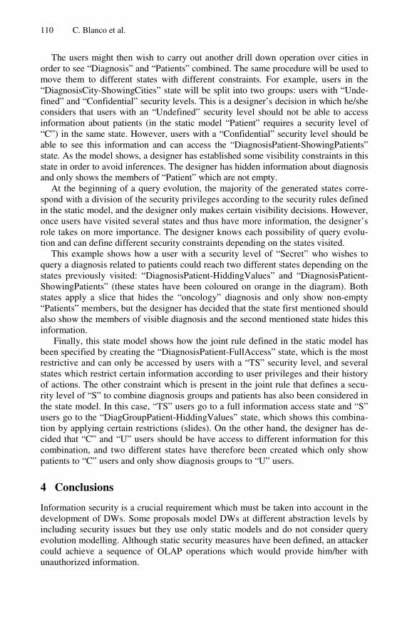
110 C. Blanco et al.
The users might then wish to carry out another drill down operation over cities in order to see “Diagnosis” and “Patients” combined. The same procedure will be used to move them to different states with different constraints. For example, users in the “DiagnosisCity-ShowingCities” state will be split into two groups: users with “Unde-fined” and “Confidential” security levels. This is a designer’s decision in which he/she considers that users with an “Undefined” security level should not be able to access information about patients (in the static model “Patient” requires a security level of “C”) in the same state. However, users with a “Confidential” security level should be able to see this information and can access the “DiagnosisPatient-ShowingPatients” state. As the model shows, a designer has established some visibility constraints in this state in order to avoid inferences. The designer has hidden information about diagnosis and only shows the members of “Patient” which are not empty.
At the beginning of a query evolution, the majority of the generated states corre-spond with a division of the security privileges according to the security rules defined in the static model, and the designer only makes certain visibility decisions. However, once users have visited several states and thus have more information, the designer’s role takes on more importance. The designer knows each possibility of query evolu-tion and can define different security constraints depending on the states visited.
This example shows how a user with a security level of “Secret” who wishes to query a diagnosis related to patients could reach two different states depending on the states previously visited: “DiagnosisPatient-HiddingValues” and “DiagnosisPatient-ShowingPatients” (these states have been coloured on orange in the diagram). Both states apply a slice that hides the “oncology” diagnosis and only show non-empty “Patients” members, but the designer has decided that the state first mentioned should also show the members of visible diagnosis and the second mentioned state hides this information.
Finally, this state model shows how the joint rule defined in the static model has been specified by creating the “DiagnosisPatient-FullAccess” state, which is the most restrictive and can only be accessed by users with a “TS” security level, and several states which restrict certain information according to user privileges and their history of actions. The other constraint which is present in the joint rule that defines a secu-rity level of “S” to combine diagnosis groups and patients has also been considered in the state model. In this case, “TS” users go to a full information access state and “S” users go to the “DiagGroupPatient-HiddingValues” state, which shows this combina-tion by applying certain restrictions (slides). On the other hand, the designer has de-cided that “C” and “U” users should be have access to different information for this combination, and two different states have therefore been created which only show patients to “C” users and only show diagnosis groups to “U” users.
4 Conclusions
Information security is a crucial requirement which must be taken into account in the development of DWs. Some proposals model DWs at different abstraction levels by including security issues but they use only static models and do not consider query evolution modelling. Although static security measures have been defined, an attacker could achieve a sequence of OLAP operations which would provide him/her with unauthorized information.

Towards the Secure Modelling of OLAP Users’ Behaviour 111
In this paper, a new kind of security rules (joint rules) has been added to our static modelling proposal in order to define sensitive combinations of information and the security privileges needed to query this information.
This approach also fulfils static models with a secure dynamic modelling. State models have been proposed in which the use of several states defines what informa-tion has to be provided in each case, by considering aspects that it is impossible to model in a static manner, such as the information that has been shown by the user (previously visited states).
Our future work is focused on the improvement of the session control to include an automatic detection of possible inferences and to recommend actions to the administrator.
Acknowledgments. This research is part of the BUSINESS (PET2008-0136) Project financed by the “Ministerio de Ciencia e Innovación” (Spain), the PEGASO/MAGO (TIN2009-13718-C02-01) Project financed by the "Ministerio de Ciencia e Innovación" (Spain) and "Fondo Europeo de Desarrollo Regional FEDER", the SISTEMAS (PII2I09-0150-3135) Project financed by the “Consejería de Educación y Ciencia de la Junta de Comunidades de Castilla-La Mancha” (Spain), the QUASIMODO (PAC08-0157-0668) Project financed by the “Viceconsejería de Ciencia y Tecnología de la Junta de Comunidades de Castilla-La Mancha” (Spain), the MEDUSAS (IDI-20090557) Pro-ject financed by the "Centro para el Desarrollo Tecnológico Industrial. Ministerio de Ciencia e Innovación (CDTI)” (Spain). Partial support from the EU project "Security Engineering for Lifelong Evolvable Systems (Secure Change)" (ICT-FET-231101) is gratefully acknowledged.
References
1. Inmon, H.: Building the Data Warehouse, 3rd edn. John Wiley & Sons, USA (2002) 2. Kimball, R.: The Data Warehouse Toolkit. John Wiley & Sons, Chichester (2002) 3. Lodderstedt, T., Basin, D., Doser, J.: SecureUML: A UML-based modeling language for
model-driven security. In: Jézéquel, J.-M., Hussmann, H., Cook, S. (eds.) UML 2002. LNCS, vol. 2460, p. 426. Springer, Heidelberg (2002)
4. Mouratidis, H., Giorgini, P.: Integrating Security and Software Engineering: Advances and Future Vision. Idea Group Publishing, USA (2006)
5. Fernández-Medina, E., et al.: Model-Driven Development for secure information systems. Information and Software Technology 51(5), 809–814 (2009)
6. Jürjens, J.: Secure Systems Development with UML. Springer, Heidelberg (2005) 7. Jurjens, J.: Principles for Secure Systems Design, PhD Thesis, Oxford University (2002) 8. Houmb, S.H., et al.: Cost-Benefit Trade-Off Analysis using BBN for Aspect-Oriented
Risk-Driven Development. In: International Conference on Engineering of Complex Com-puter Systems (ICECCS), pp. 195–204. IEEE Computer Society, Shanghai (2005)
9. Thuraisingham, B., Kantarcioglu, M., Iyer, S.: Extended RBAC-based design and imple-mentation for a secure data warehouse. International Journal of Business Intelligence and Data Mining (IJBIDM) 2(4), 367–382 (2007)
10. Priebe, T., Pernul, G.: A Pragmatic Approach to Conceptual Modeling of OLAP Security. In: Kunii, H.S., Jajodia, S., Sølvberg, A. (eds.) ER 2001. LNCS, vol. 2224, p. 311. Springer, Heidelberg (2001)

112 C. Blanco et al.
11. Fernández-Medina, E., Trujillo, J., Piattini, M.: Model Driven Multidimensional Modeling of Secure Data Warehouses. European Journal of Information Systems 16, 374–389 (2007)
12. Saltor, F., et al.: Building Secure Data Warehouse Schemas from Federated Information Systems. In: Bestougeff, H., Dubois, J.E., Thuraisingham, B. (eds.) Heterogeneous Inf. Exchange and Organizational Hubs, pp. 123–134. Kluwer Academic Publisher, Dordrecht (2002)
13. Trujillo, J., et al.: A UML 2.0 Profile to define Security Requirements for DataWare-houses. Computer Standard and Interfaces 31(5), 969–983 (2009)
14. Trujillo, J., et al.: An Engineering Process for Developing Secure Data Warehouses. In-formation and Software Technology 51(6) (2009)
15. Fernández-Medina, E., et al.: Access Control and Audit Model for the Multidimensional Modeling of Data Warehouses. Decision Support Systems 42, 1270–1289 (2006)
16. Soler, E., et al.: Building a secure star schema in data warehouses by an extension of the relational package from CWM. Computer Standard and Interfaces 30(6), 341–350 (2008)
17. Blanco, C., et al.: Applying QVT in order to implement Secure Data Warehouses in SQL Server Analysis Services. Journal of Research and Practice in Information Technol-ogy 41(2), 135–154 (2009)
18. Fernández-Medina, E., et al.: Developing Secure Data Warehouses with a UML extension. Information Systems 32(6), 826–856 (2007)

A Formal P3P Semantics for Composite Services
Assadarat Khurat1, Dieter Gollmann1, and Joerg Abendroth2
1 Hamburg University of Technology,Harburger Schlossstr. 20, 21079 Hamburg, Germany
[email protected], [email protected] Nokia Siemens Networks,
St.Martin-str.53, 81669 [email protected]
Abstract. As online services are moving from the single service to thecomposite service paradigm, privacy is becoming an important issue dueto the amount of user data being collected and stored. The Platformfor Privacy Preferences (P3P) was defined to provide privacy protectionby enabling services to express their privacy practices, which in turnhelps users decide whether to use the services or not. However, P3P wasdesigned for the single service model, bringing some challenges whenemploying it with composite services. Moreover the P3P language maylead to misinterpretation by P3P user agents due to its flexibility and mayhave internal semantic inconsistencies due to a lack of clear semantics.Therefore, we enhance P3P to be able to support composite services,propose a formal semantic for P3P to preserve semantic consistency, andalso define combining methods to obtain the privacy policies of compositeservices.
Keywords: formal semantics, P3P, privacy policy, composite service.
1 Introduction
In the beginning of the online services era, most services were single and indepen-dent, employing and developing proprietary technology to serve their customers.Nowadays, there is strong competition in the online market to expand the num-ber of customers. This is an incentive for developing new and better services tobetter serve user demands. It is then a promising approach to build new servicesby combining existing services which can reduce development cost and time com-pared to implementing a new service from scratch. Thus, one can say that theonline service world now has changed from single to composite services [12].
In online services, privacy is an important issue due to the large amount ofuser data collected and stored. Users need some mechanism to secure their data.To protect privacy, users ought first to be aware of what the services will do withtheir data so that they can decide whether to use the services or not. This facilityis provided by the Platform for Privacy Preferences (P3P) [1], a policy languagefor describing data practices of websites. Comparing these practices with the
W. Jonker and M. Petkovic (Eds.): SDM 2010, LNCS 6358, pp. 113–131, 2010.c© Springer-Verlag Berlin Heidelberg 2010

114 A. Khurat, D. Gollmann, and J. Abendroth
users’ preferences, expressed, e.g., in the P3P Preference Exchange Language(APPEL) [5], thus helps users to protect their privacy to a certain degree.
When applying P3P policy for composite services, some challenges are raised.For example, P3P was originally designed for the single service model, how canwe obtain the P3P policy of a composite service consisting of several services isone challenge. Besides, P3P policy from some service members may be conflictwith each other. How can these discrepancies be detected is another challenge.From these challenges, we enhance P3P so that it can handle composite servicescenario and we also define constraints to analyse conflicts between the privacypolicies of service members. This analysis also helps avoiding a combination ofservices with incompatible privacy policies, which will fail at run-time. Moreover,a combining scheme is also proposed to obtain privacy practices of the compositeservice.
The semantics of the P3P language is ambiguous so that the same P3P pol-icy can be interpreted differently by different user agents [2,10]. This potentialsemantic inconsistencies of a P3P policy elaborated in [2,3,4,9,11] will be in-herited to the composite service consisting of services the ambiguous statementbelongs to. We, therefore, consider formal semantics for P3P so that semanticconsistency can be preserved. Our formal semantics for P3P is based on workfrom T. Yu et al.[2] which proposed a data centric formal semantics for P3P byemploying relational tables. They claim that in some cases it does not dependon purpose whether or not the collected data is used. We, however, argue thatpurpose is important to notify the reason for data collection. Thus, data-purposecentric is used in our formal semantics P3P.
The organization of this paper is as follows. Section 2 describes the P3P syn-tax, its possible semantic inconsistencies and P3P in composite service. Theenhancement of P3P is proposed in Section 3. A formal semantics of P3P andconstraints for inconsistency verification are shown in Section 4. Section 5 indi-cates a combining algorithm for composite services. An example of this algorithmis presented in Section 6. Related work is discussed in Section 7 and we concludeour paper in Section 8.
2 The Platform for Privacy Preferences
The Platform for Privacy Preferences (P3P) [1] is an XML-based policy lan-guage specified by W3C to enable websites to describe their privacy practices ina standard format. Users can compare P3P policy of a website with their prefer-ences before making a decision whether to use the website. This comparison canbe done automatically by a P3P user agent installed at the users’ side, e.g. bya web browser. The P3P specification defines syntax and semantics of the P3Ppolicies, mechanisms for associating policies with web resources, e.g. by HTTP,and a standard set of data elements in a hierarchy which all P3P user agentsshould understand.

A Formal P3P Semantics for Composite Services 115
2.1 P3P Syntax
The main elements of P3P policy are ENTITY, ACCESS, DISPUTES-GROUPand STATEMENT. In a policy, there are an ENTITY element identifying a legalentity, i.e. a service or website issuing this policy, an ACCESS element indicatingthe ability of individuals to access their data, a DISPUTES-GROUP describingthe resolution procedure when disputes about this privacy practices occur, andone or more STATEMENT elements illustrating possible usage of the websiteregarding data elements. P3P also defines categories for its defined standard setof data elements such as physical (e.g. name)and online (e.g. email address).These base data are structured in hierarchy. An example of P3P statementsof Superpages [13] website that is a service providing search function for e.g.restaurants in desired location is illustrated in Fig. 1.
Statement1 { purpose: admin, current, develop
recipient: ours
retention: indefinitely
data: #dynamic.clickstream, #dynamic.http,
#dynamic.searchtext}Statement2 { purpose: develop, tailoring
recipient: ours
retention: business-practices
data: #dynamic.cookies [optional] (category: uniqueid)}
Fig. 1. P3P Statements of Superpages Website
In a STATEMENT, the major elements are data, purpose, recipient and re-tention. The data element expresses data and possibly its category the servicesmay collect. For which purpose and for how long the data is collected canbe described by the purpose and retention elements respectively. P3P definesfive retention values, no-retention, stated-purpose, legal-requirement,business-practice and indefinitely. Brief descriptions as defined in P3P1.1 are given in Table 1. In some cases services distribute data collected to thirdparties. This can be specified in the recipient element. P3P defines six values forthis element, ours, same, delivery, other-recipient, unrelated and public.Their short descriptions as defined in P3P 1.1 are given in Table 2.
For data, purpose and recipient elements, there is an attribute describingwhether they are required for the website or optional. P3P 1.1 defines an ex-tension element called STATEMENT-GROUP-DEF helping in indicating whichstatement belongs to the same group of user interactions with the services. Ser-vices can also define usages of the same statement group to opt-in or opt-out viathe consent attribute of this element.
P3P allows multiple data elements, multiple purpose values, multiple recipi-ent values and a retention value in one statement. This means the stated dataelements can be employed for all stated purposes, can be distributed to all listed

116 A. Khurat, D. Gollmann, and J. Abendroth
Table 1. Descriptions of P3P Retention Values
Retention Values Descriptions
no-retention Information is not retained for more than a brief periodof time necessary to make use of it during the course ofa single online interaction.
stated-purpose Information is retained to meet the stated purpose. SitesMUST have a retention policy that establishes a destruc-tion time table. The retention policy MUST be includedin or linked from the site’s human-readable privacy pol-icy.
legal-requirement Information is retained to meet the stated purpose butthe retention period is longer because of a legal require-ment or liability. Sites MUST have a retention policy thatestablishes a destruction time table. The retention policyMUST be included in or linked from the site’s human-readable privacy policy.
business-practices Information is retained under a service provider’s statedbusiness practices. Sites MUST have a retention policythat establishes a destruction time table. The retentionpolicy MUST be included in or linked from the site’shuman-readable privacy policy.
indefinitely Information is retained for an indeterminate period oftime.
Table 2. Descriptions of P3P Recipient Values
Recipient Values Descriptions
ours Ourselves and/or entities acting as our agents or entitiesfor whom we are acting as an agent
same Legal entities following our practices
delivery Delivery services possibly following different practices(may use data other than stated purpose including deliv-ery services with unknown data practices)
other-recipient Legal entities following different practices
unrelated Unrelated third parties (data usage practices are un-known)
public Public fora
third party recipients, and are stored as long as defined in the retention policy.Besides, P3P allows specifying the same data elements in more than one state-ment. This flexibility on one hand brings expressiveness to the policy. However,on the other hand it may also cause semantic inconsistency problems.

A Formal P3P Semantics for Composite Services 117
2.2 Potential Semantic P3P Inconsistencies
There exist possible semantic inconsistencies due to non-corresponding betweenvalues of some elements of P3P policy, which were elaborated in [2,3,4,9,11]. Webriefly describe them in the following.
Conflict between purpose and data category: For example, a statement containspurpose value individual-analysis but does not contain any data elementfrom one of physical, online, financial, purchase and government datacategories. This does not make sense since the purpose individual-analysisrequires identified data. Similar conflicts are listed in [3] and in the P3P 1.1specification (User Agent Guidelines).
Conflict between purpose and retention: For instance, a statement contains pur-pose value develop and retention value no-retention. This introduces a conflictsince no-retention allows data to be stored only for a brief period of time whichis less than develop requires.
Conflict between purpose and recipient: For example, when a statement containspurpose values admin, develop and/or tailoring with recipient values onlydelivery, same or public. This does not make sense since according to thespecified purposes, the recipient value ours must be present.
Conflict between recipient and retention: in a statement, some defined recip-ient values do not correspond to some retention values. When, for instance,a statement contains recipient value public and a retention value other thanindefinitely.
Optional attributes: With attributes expressing whether data, purpose and re-cipient elements are required or optional, ambiguities may exist, for examplewhen data is required while purpose and recipient are optional. It is unclearwhether the data is collected or not at first. In cases when the STATEMENT-GROUP-DEF element is employed, the value of these attributes in the statementbelonging to the group must correspond to the value of the consent attribute.
With these possible conflicts, it is not trivial to write P3P policies withoutconsiderably caution to be able to protect semantic consistency. Thus, there isa need for formal semantics for P3P to mitigate this problem. For each type ofconflict above, there could be more cases introducing semantic inconsistenciesin P3P policies. However, our work is focusing on formal semantic for P3P forcomposite service. Finding out all cases of these conflicts is out of scope forour work. We neither consider discrepancies between P3P policy and its naturallanguage.
2.3 P3P Policy in Composite Services Analysis
Composite services come from Service Oriented Architecture (SOA) approach. Acomposite service consists of multiple services, being single or composite. Each

118 A. Khurat, D. Gollmann, and J. Abendroth
service is seen as a component that is loosely coupled and make use of data fromother services in the combination to provide a new service. The service composi-tion is supported by technologies e.g. BPEL [6], WSDL, etc. Recently, a methodto combine also web-based services called “mashup” was proposed in [12].
P3P defined recipient value to describe which type of third party the collecteddata may be distributed to. In a composite service, some data are transferredbetween service members. Thus the services receiving data become third partyservices of the data sender service. However, noticing from descriptions of re-cipient values, it could be implied that the recipient values can be determinedwhen the recipient services (third party services) are known by the data senderservice. In a service composition process, which services are selected as mem-bers depends on targets and goals of the desired composite service. Thus, wewill never know which services will be combined together beforehand. With thisdynamic characteristics, there might be unknown services in the combination.Thus, none of the existing recipient values can be used to capture these services.
Basically, each of service members has its own P3P policy. With the singleservice approach, comparing a user’s preferences with P3P policies from all singleservices is done one by one. However, in a combination this is not sufficientsince there might be conflicts between the privacy policies of services. The P3Pframework does not provide any mechanism regarding this issue. For example,when privacy policy of Service A does not allow sending data needed by ServiceB in providing a composite service, thus, this composite service cannot function.
The comparison between users’ preferences and privacy practices of the web-sites are normally done at the user agent, i.e. at the user side. Obtaining theprivacy policy of the composite service allows this analysis to occur only onceresulting in less resource consumption at the end-users than with the formerapproach. In addition, this privacy policy of the composite service can be usedfor further service compositions in the future.
3 P3P Enhancements
In order for P3P to support the composite service paradigm, we enhance P3P inthree points. We define a new recipient value, require a third party service listfor recipient values, and define a destruction time table for retention policies.The last two extensions facilitate in deriving privacy policy of composite service.
3.1 Recipient Value
Since the existing P3P recipient values are not sufficient for composite service,wepropose a new recipient value, “prospective-composite-service”, to fill thisgap. Similar to all recipient values besides ours, this value can have a requiredattribute. The new recipient value serves as a placeholder for future services ina composite service, implying that the data may be distributed to legal enti-ties that are members of the prospective composite service but with the users’consent. With this value service providers can express their recipient value for

A Formal P3P Semantics for Composite Services 119
prospective services that are not known before enabling service composition.Hence, the new composite service can be successfully created but the data ofthe users who are using a service in the composite service are not distributed toother service members without the users’ consent.
3.2 Third Party Service List
Existing single service defines recipient values of data based on privacy practicesof the data’s recipients whether they are the same, different, unknown, etc. tothe original service itself. Therefore, each single service has its own scope todetermine the recipient value which is different from the others. In order tospecify the recipient value of a composite service, it is necessary to find outthe scope of recipient values of the composite service in which the scope ofall service members must be taken into account. However, since each memberhas different scope, some recipients of a recipient value of a particular data ofa service may overlap which makes it extremely hard to resolve the recipientvalues of the composite service instead of just combining all recipient values ofthe data in case of non-overlapping. For example, let a composite service consistsof service A and service B. For a particular data, service A has a recipient valueother-recipient. The recipients of other-recipient of service A may includeservice B or some recipients that have the same privacy practices as service Bor some recipients that have different privacy practices as service B, resulting invarious possible or insolvable recipient values for the composite service dependingon the recipient value of service B.
This problem can be solved if we know exactly the recipients in which wecall “third party services” belonging to the recipient values of each servicemember. Therefore besides prospective-composite-service and public, werequire that there must be a list of third party services attached to each re-cipient value of a particular data. We expect that this will not be a difficulttask for service providers since it is necessary to know the third party ser-vices such that they could specify their recipient values. The defined lists forours, same, delivery, other-recipient and unrelated values are called “ours-list”, “same-list”, “delivery-list”, “other-recipient-list” and “unrelated-list” re-spectively. The ours-list from single service contains its own service. We alsodefine another list called “service-member-list” containing all member servicesof the composite service. In addition, in case of services with known privacypractices their P3P policies must be available.
Since the recipient values of existing P3P policies, i.e. without the third partyservice list, are defined coarse-grained and with single service environments, theP3P policies of a service provider will not change often. On the other hand,P3P policies with a third party service list which could be altered dynamicallymay have to be updated more frequently. This might be inconvenient especiallyfor the users who normally have to approve the new list every time it changes.However, knowing the list helps the users to protect their data disclosure tounwanted third party services both when they first check whether to use thisservice or not and later when the list changes. In addition, if the service provider

120 A. Khurat, D. Gollmann, and J. Abendroth
allows the users to specify a third party service black list e.g. at subscriptiontime, when the list changes the service providers can obtain the users’ decisionautomatically whether they agree with the new list or not without contactingthe users again.
3.3 Destruction Time Table
It is also not trivial to determine the retention value for a composite service. Forexample, though two services specify their retention value as stated-purpose,it does not mean they store the data for the same period of time. It is even harderto combine retention values between stated-purpose, legal-requirement andbusiness-practices since they are incomparable. A possible way to solve thisproblem is to know the exact length of the retention time. P3P policy is spec-ified that for retention values; stated-purpose, legal-requirement andbusiness-practices, there must be a retention policy establishing a destructiontime table included in or linked from the site’s human-readable privacy policybut it does not further define what the retention policy looks like. To us, it isforeseeable that this destruction time table can be employed to resolve the reten-tion value for composite service. We thus propose that the P3P policy from eachservice must have a destruction time table as shown in Table 3 for the retentionvalues stated-purpose, legal-requirement and business-practices.
The destruction time table expresses how long a service stores a particulardata using the dayTimeDuration type. As stated in the P3P specification forstated-purpose and legal-requirement, the determination of the durationtime depends on the purpose element. For business-practices, P3P statesthat the retention policy can be “determined by service provider’s business prac-tices” [1]. We suggest to base the retention duration of business-practices also
Table 3. Destruction Time Table
Retention Value Purpose Retention Duration (dayTimeDuration)
stated-purpose
current PT10Madmin P3Mdevelop P3Mtailoring P3M
legal-requirement
current P6Madmin P6Mcontact P2Yhistorical P2Ytelemarketing P2Y
business-practices
current P3Madmin P5Mtailoring P3Mdevelop P6Mpseudo-decision P1Y

A Formal P3P Semantics for Composite Services 121
on purpose. Thus, for each retention value in the table, the retention durationis determined for each applied purpose value. Not all purpose values may bepresent since the service may not use the data for that purpose.
4 Formal Semantics for P3P in Composite Services
In our formal semantics for P3P in composite service environments, we assumethat the conflicts illustrated in Section 2.2 have already been analysed. Thus,the P3P policies obtained from each service have no conflicts on those issues. Inthis section, we show how to provide formal semantics of P3P and describe someconstraints to further verify inconsistencies of privacy policies in each serviceand also between services.
4.1 Data-Purpose Centric Semantics for P3P
To provide formal semantics for P3P, we use the same technique as in [2] i.e.employing a relation database. However, instead of following a data-centric ap-proach, we will use data-purpose (dp) as the key for our relation table. Thereason is that purpose is an important criterion for data usage. For example,to determine whether a data element is required depends pretty much on thepurpose the data is being employed for.
For each data element, P3P defines an attribute “optional” to specify whetherthe data is required by the services. The value of this attribute can be either yes(optional) or no (required). The default value is no. For this relation we define arelation table data-purpose-optional (DPO). In addition, each data element canbelong to several categories. We define another relation table for this relation asdata-purpose-category (DPC).
Similar to the optional attribute of data element, for each purpose value exceptcurrent P3P defines an attribute “required” describing whether it is required.There are three values of this attribute, i.e. always (required), opt-out (usersmust request to not use the data for this purpose) and opt-in (data may onlybe used for this purpose if the users have agreed). The default value when norequired attribute is present is always. We define a relation table for this relationas data-purpose-required (DPR).
How long a particular data element should be stored as expressed by the re-tention element depends on the purpose the data is being utilized for. Accordingto our P3P enhancement in Section 3.3, each retention value for a purpose valuehas a duration time. We define a relation table of this relation as data-purpose-retention-duration (DPRD). The duration represents the retention duration timederived from the destruction time table as defined in Section 3.3.
To whom a particular data may be distributed depends also on the purposeof usage. As same as purpose element, each recipient value except ours canhave a required attribute, i.e. always, opt-out or opt-in. The default valuewhen no required attribute is present is always. Extending with the third partyservice lists, we define a relation table for this relation as data-purpose-recipient-third party service-required (DPRTR).

122 A. Khurat, D. Gollmann, and J. Abendroth
Table 4. Details of Relation Tables
Relation Tables Fields Key of the relation
DPOdata (data,purpose)purposeoptional
DPRdata (data,purpose)purposerequired
DPCdata (data,purpose,category)purposecategory
DPRD
data (data,purpose)purposeretentionduration
DPRTR
data (data,purpose,recipient,purpose third party service)recipientthird party servicerequired
service-entity
ENTITY (#business.name) (ENTITY)ACCESSDISPUTES (resolution-type)DISPUTES (REMEDIES)
We also rewrite the ENTITY, ACCESS and DISPUTES-GROUPS elementsin a table called service-entity. The key element of this table is ENTITY,#business.name of the service. The details of these tables are shown in Table 4.
4.2 Constraints for Integrity Verification
We use similar constraints as shown in [2] and an additional constraint accordingto the data-purpose centric approach to ensure the integrity of P3P policies foreach service as follows:
Multiple statements for a data element: P3P allows specifying more than onestatement for the same data-purpose. Thus, multiple retention values can beassigned to the same data-purpose. For two tuples having the same data-purposevalues, it does not make sense to have several retention values. If this is the case,the policy is considered invalid. This can be applied also for the DPO, DPR andDPRTR relations.
∀p, q ∈ DPRD, p.(data, purpose) = q.(data, purpose)→ p.retention = q.retention
Data hierarchy: in P3P, data is structured in a hierarchy. It does not makesense if the upper level (e.g. #user.bdate) has more restrictions than its lower

A Formal P3P Semantics for Composite Services 123
level (e.g. #user.bdate.ymd.year). For instance, if the data optional attributeof #user.bdate is optional, the data optional attribute of #user.bdate.ymd.yearcan be optional or required. But if the data optional attribute of #user.bdate isrequired, the data optional attribute of #user.bdate.ymd.year must be required.This concept can be applied to DPR and DPRTR relations.
∀p, q ∈ DPO, p.data is the upper level of q.data, p.optional = no→ q.optional = no
Purpose and data optional constraints: if the purpose value of a data is current,the optional value of that data must be no since it is necessary that the datamust be collected. Otherwise the service cannot be provided.
∀p ∈ DPO, p.purpose = current → p.optional = no
4.3 Constraints for Integrity Verification between Services
In the composite service environment, several single services and/or compositeservices cooperate with each other to perform a service. Hence, input data ofone service can be output of other services. This may introduce conflicts whena service supposed to send data as an input to another service does not do itdue to its privacy policies. Thus, we first have to find out which personal datais transferred between services. Then we further analyse its privacy policies forboth sender and recipient services.
The personal data transferred can be derived e.g. from a WS-BPEL [6] de-scription of a service. How the personal data are derived is out of scope of ourwork. In the following, the data structure shared with components shared.dataand shared.provider will hold the personal data shared between services and theirproviders. For personal data items with more than one provider there would beseveral entries. We define constraints to check the conflicts for each service mem-ber of a composite service as follows:
Data collection: the data used between services are obviously needed to fulfillthe service provisioning, thus their collection must be required. Otherwise, thiscomposite service cannot function.
∀p ∈ DPO, p.data ∈ shared.data → p.optional = no
Purpose: for the same reason as for data collection, the purpose values of thesedata must contain at least current value with required value as always.
∀p ∈ DPR, p.data ∈ shared.data → p.purpose = current ∧ p.required = always
Recipient: if the recipient value of the transferred data of the sender servicecontains at least prospective-composite-service, the combination is feasible.

124 A. Khurat, D. Gollmann, and J. Abendroth
Let DPRTRi be the DPRTR table for provider (i). We check the followingconstraints on that data:
∀p ∈ DPRTRi, (p.data, i) ∈ shared→ p.recipient = prospective-composite-service
If the recipient value of the transferred data contains only ours, this means thatthe service does not send that data to other parties. Thus, the composite servicecannot function. In other cases, the third party service list must be checked.If the recipient service is not in the list as specified, this service combinationcannot function.
∀p ∈ DPRTRi, (p.data, i) ∈ shared → p.recipient �= ours
5 Combining Mechanism
We determine relation tables for the composite service (CS) by combining thesame table type of each member service. For each type of table we add alltuples from all services that have different data-purpose values into a new tablei.e. belonging to the composite service. Let dp be (data, purpose) attributesin relations. For tuples having the same dp values, the following combinationschemes are applied before adding them into the new table:
a) data-purpose-optional (DPO)It does not make sense for a service to specify several values for the dataoptional attribute of a data-purpose value. As we assume that the P3P policyfrom each service is validated beforehand, the optional value for a dp fromeach service must be only one value, either yes (optional) or no (required).For the same reason, the optional value of a dp for a composite service mustbe only one value.
With n tuples from DPO (dp1,optional1), (dp2,optional2),. . . , (dpn,option-aln) having the same data-purpose (dp1 = dp2 = · · · = dpn), we define thatthe optional value of the composite service is the most restrictive one (no>yes). This means if at least one of the optional values is no then theoptional value of the composite service is no, otherwise yes.
From the same reason shown in Section 4.2, data hierarchy is also con-sidered. With two data elements, if optional value of the upper level datahas higher restriction than the lower one, the optional value of the lower onemust be changed to be the same as the upper level data.
b) data-purpose-required (DPR)This required value represents the requirement of the purpose element. Sim-ilarly to data optional, the required value of a dp from each service must beonly one value i.e. always, opt-out or opt-in. With n tuples from DPR(dp1,required1), (dp2,required2),. . ., (dpn,requiredn) having the same data-purpose (dp1 = dp2 = · · · = dpn), the required value of the composite serviceis the most restrictive one (always >opt-out >opt-in).

A Formal P3P Semantics for Composite Services 125
c) data-purpose-category (DPC)A data-purpose relation can have several category values. Since we assumethat possible inconsistencies between purpose and data category are vali-dated beforehand, this conflict will not occur when combining P3P policiesfrom different services. With n tuples from DPC (dp1,category1), (dp2,cate-gory2),. . ., (dpn,categoryn) having the same data-purpose (dp1 = dp2 = · · ·= dpn), the category value of the composite service (categoryCS) can beobtained as the union of the category values from all of them (categoryCS =category1∪ category2 ∪ · · · ∪ categoryn).
d) data-purpose-retention-duration (DPRD)As previously described in Section 3.3, it is not trivial to combine retentionvalues for a composite service. The duration value derived from destructiontime table can help in determining the retention value as below.
Similar to the optional and required attributes for a data-purpose relationfrom a service, the retention value must be only one value. With n tu-ples from DPRD (dp1,retention1,duration1), (dp2,retention2,duration2),. . .,(dpn,retentionn,durationn) having the same data-purpose (dp1 = dp2 =· · · = dpn), the retention value of the composite service is the most re-strictive one (indefinitely > business-practices, legal-requirement,stated- purpose > no-retention). Due to the fact that business-prac-tices, legal-requirement and stated-purpose are incomparable, therecan be cases where the retention value cannot be resolved by using only thisconstraint. Thus the duration time comes into play.
Since the retention value describes how long the service keeps the data,we consider the longest storing period and its retention value to become theretention duration and retention value of the composite service respectively.For example, let the purpose for collecting a particular data be admin and theretention value of the first service be stated-purposewith a retention dura-tion of three months, while the second service collects the same data for thesame purpose for six months with the retention value business-practices.The retention value and its duration of the composite service for this data-purpose relation is business-practiceswith six months duration due to thelonger time duration. In case when the retention duration from both is equal,we consider the one with the most restrictive meaning (business-practices>legal-requirement >stated-purpose).
e) data-purpose-recipient-third party service-required (DPRTR)The recipient is quite a complicated element when considered in a compositeservice. Though it is possible for a data-purpose relation to have severalrecipient values, determining the recipient value for the composite serviceis not possible by just simply taking the union of the recipient values fromall services having the same data-purpose relation as previously described inSection 3.2. Therefore, we use the third party service list in determining therecipient value of the composite service.
Besides the recipient value of the composite service and the required valueof each recipient value, we also have to find out the member services of

126 A. Khurat, D. Gollmann, and J. Abendroth
each list. Unlike the first four relations that the tuples having different data-purpose values are added in the new table belonging to composite servicewithout further processing. Due to the different scope of single service andcomposite service, all tuples of DPRTR relation after being added in thenew table are analysed. The recipient value, its required value and memberservices of each third party service list of the composite service can be derivedin the following steps:
1. For each recipient value (except prospective-composite-service andpublic), there is a list of third party services attached as well as arequired value. We attach this required value to every third party ser-vice in the list (tps-required). For the tuples of DPRTR table from allservices having different data-purpose (dp) values, first they are addedinto the new table waiting for further processing as shown in the follow-ing steps. With n tuples from DPRTR (dp1,recipient1,tps1,required1),(dp2,recipient2,tps2,required2), . . . , (dpn,recipientn,tpsn,requiredn) hav-ing the same data-purpose (dp1 = dp2 = · · · = dpn), we combine theirrecipient value by using union before adding them in the new table.For each recipient value, we also take the union to combine the thirdparty services associated with. Each third party service can have onlyone required value. With n tuples from tps-required (tps1,required1),(tps2,required2),. . ., (tpsn,requiredn) having the same service (tps1 =tps2 = · · · = tpsn), the required value is the most restrictive one (always>opt-out >opt-in). In this step, if the recipient values contain public,then public is one of the recipient values for the composite service re-spectively. The required value of recipient value public is the most re-strictive one (always >opt-out >opt-in).
2. Since the scope of recipient values from each member service of the com-posite service may be different, there might be some third party servicesin same-list, delivery-list, other-recipient-list and unrelated-list belongingto the member of the composite service. This overlapping must be elim-inated. We thus check services in each list with the service-member-listwhether they are redundant. If there are, those services must be removedfrom their current lists. This also implies that the recipient value oursis one of the recipient value for the composite service.
3. In addition, there might be some third party services in delivery-list,other-recipient-list and unrelated-list that have the same privacy prac-tices as the composite service. We thus check this case in two steps. Firstwe check if there are any services in delivery-list, other-recipient-list andunrelated-list that are the same as the services in the same-list. If thereare, those services must be removed from their current lists. Secondly wealso have to check whether the remaining services in those lists have thesame data practices as the composite service or not by verifying their pri-vacy policies against the privacy policies of the composite service whichwill be explained later. If any of these services conform to the compos-ite service’s privacy policies, they are moved to the same-list. In case

A Formal P3P Semantics for Composite Services 127
there are no privacy policies available (i.e. all services in unrelated-listand some services in delivery-list) or the services do not conform to thecomposite service’s privacy practices, they are left in their current lists.We do not have to check redundancy of services between delivery-list,other-recipient-list and unrelated-list since from the definitions they donot overlap with each other.
4. For the ours-list, same-list, delivery-list, other-recipient-list andunrelated-list, if they are not empty, then their corresponding recipient values, i.e.ours, same, delivery, other-recipientand unrelated respectively areone of the recipient values for the composite service and they become alsothe third party service lists of the composite service. Here there could beseveral required values attached to services in each list coming from differ-ent member services, the new required value of the recipient values for thecomposite service is themost restrictive one (always>opt-out>opt-in).
5. For the recipient value prospective-composite-service, since now thescope is different than from the single service, we remove this recipientvalue associated with data that are not the output of the compositeservice. These data can be derived from e.g. WS-BPEL.
Regarding the checking of the same privacy practices in step 3, by now wealready obtained the first four relation tables of the composite service i.e.DPO, DPR, DPC and DPRD. The verification between the privacy policiesof the remaining services in delivery-list, other-recipient-list and unrelated-list and the privacy practices of the composite service is done by checkingwith these four relation tables and with restricted recipient values. For adata-purpose relation if the optional value, required value, category valueand retention value of the remaining services in those lists are equal or lessrestrictive than the optional, required, category and retention values of thecomposite service respectively and if the recipient values of the services inthose lists contain only ours or same or both, this implies that their privacypolicies conform to the composite service. We do not take the required valueof the recipient value same into consideration, since even if it is required, therecipient services in the same-list still have the same privacy practices as thecomposite service.
For the service-entity table, we can obtain the table of the composite serviceby just concatenating every row from each service into one table.
6 Example
In this section, we present a scenario to obtain privacy policy of a potential compos-ite service, Restaurantlocator. The Restaurantlocator service may consist of Su-perpages and GPS-data-stream [14] services. Given a city name in United States, alist of restaurants can be obtained from the Superpages. After choosing the restau-rant users want to visit, the GPS-data-stream provides a point of interest file con-taining exact location of the restaurant which can be directly loaded to users’ GPSdevice. P3P statement of GPS-data-stream is shown in Fig.2.

128 A. Khurat, D. Gollmann, and J. Abendroth
Statement { purpose: admin, current, develop
recipient: ours
retention: indefinitely
data: #dynamic.clickstream, #dynamic.http,
#dynamic.cookies (category: navigation, online)}
Fig. 2. P3P Statement of GPS-data-team
Due to the limitation of space, we give example in P3P statement instead ofwhole policy and with only one data, #dynamic.clickstream. In order to obtainprivacy policy of the Restaurantlocator, existing P3P policies of both Superpagesand GPS-data-stream must be extended beforehand. The privacy practices of Su-perpages and GPS-data-stream services for data, #dynamic.clickstream, aremapped to relation tables DPO, DPR, DPC, DPRD and DPRTR with their com-bining result belonging to composite service, Restaurantlocator, as illustrated inTable 5,6,7,8,9 respectively.
From all relation tables, an overlapping of data and purpose values betweenSuperpages and GPS-data-stream services is data #dynamic.cookies with pur-pose value develop. For the DPO relation in Table 5 and DPR relation in Table 6,the optional and required values for the Restaurantlocator of the data are no andalways correspondingly according to the rules that the most restrictive value ischosen as proposed in Section 5. For the DPC relation in Table 7, the category val-ues for Restaurantlocator of the overlappingdata can be derived by applying unionfunction. Deploying the retention duration values from the Destruction time tablein Table 3 for Superpages service, the duration of purpose values, develop andtailoring, are six months and three months. Since the retention value of GPS-data-stream for the purpose value, develop, is indefinitely, the retention valueof composite service shown in Table 8 for that data becomes indefinitely. In theTable 9 expressingDPRTR relation, since all the recipient values from both servicemembers are ours, further checking on whether the third party services have thesame or different privacy practices is not needed and the required values of all dataare always. For the #dynamic.clickstream data with purpose value , develop,of Restaurantlocator, both service members are in its ours-list.
Table 5. Data-Purpose-Optional (DPO) Relation
Data Purpose Optional
Superpages#dynamic.cookies develop yes
#dynamic.cookies tailoring yes
GPS-data-stream#dynamic.cookies admin no
#dynamic.cookies current no
#dynamic.cookies develop no
Restaurantlocator
#dynamic.cookies admin no
#dynamic.cookies current no
#dynamic.cookies develop no
#dynamic.cookies tailoring yes

A Formal P3P Semantics for Composite Services 129
Table 6. Data-Purpose-Required (DPR) Relation
Data Purpose Required
Superpages#dynamic.cookies develop always
#dynamic.cookies tailoring always
GPS-data-stream#dynamic.cookies admin always
#dynamic.cookies current always
#dynamic.cookies develop always
Restaurantlocator
#dynamic.cookies admin always
#dynamic.cookies current always
#dynamic.cookies develop always
#dynamic.cookies tailoring always
Table 7. Data-Purpose-Category (DPC) Relation
Data Purpose Category
Superpages#dynamic.cookies develop uniqueid
#dynamic.cookies tailoring uniqueid
GPS-data-stream
#dynamic.cookies admin navigation
#dynamic.cookies admin online
#dynamic.cookies current navigation
#dynamic.cookies current online
#dynamic.cookies develop navigation
#dynamic.cookies develop online
Restaurantlocator
#dynamic.cookies admin navigation
#dynamic.cookies admin online
#dynamic.cookies current navigation
#dynamic.cookies current online
#dynamic.cookies develop navigation
#dynamic.cookies develop online
#dynamic.cookies develop uniqueid
#dynamic.cookies tailoring uniqueid
Table 8. Data-Purpose-Retention-Duration (DPRD) Relation
Data Purpose Retention Duration
Superpages#dynamic.cookies develop business-practices P6M#dynamic.cookies tailoring business-practices P3M
GPS-data-stream#dynamic.cookies admin indefinitely
#dynamic.cookies current indefinitely
#dynamic.cookies develop indefinitely
Restaurantlocator
#dynamic.cookies admin indefinitely
#dynamic.cookies current indefinitely
#dynamic.cookies develop indefinitely
#dynamic.cookies tailoring business-practices P3M

130 A. Khurat, D. Gollmann, and J. Abendroth
Table 9. Data-Purpose-Recipient-Third party service-Required (DPRTR) Relation
Data Purpose Recipient Third party service Required
Superpages#dynamic.cookies develop ours Superpages always
#dynamic.cookies tailoring ours Superpages always
GPS- #dynamic.cookies admin ours GPS-data-stream always
data- #dynamic.cookies current ours GPS-data-stream always
stream #dynamic.cookies develop ours GPS-data-stream always
#dynamic.cookies admin ours GPS-data-stream always
Restaurant- #dynamic.cookies current ours GPS-data-stream always
locator #dynamic.cookies develop ours GPS-data-stream always
#dynamic.cookies develop ours Superpages always
#dynamic.cookies tailoring ours Superpages always
7 Related Work
T. Yu et al. proposed a data centric relational semantics database for P3Pin [2]. They discussed potential semantic inconsistencies of P3P policies and alsodefined some integrity constraints to validate the policy, i.e. data-centric con-straints, data hierarchy constraints and semantic vocabulary constraints. Ourwork was inspired by them. However, we use a data-purpose centric approachsince it is more appropriate and can better reflect the P3P policies.
M. Schunter et al. suggested augmenting P3P elements, i.e. retention by aconcrete time-span and recipient by a contact address [4,9]. Our work also en-hances P3P similarly for retention but for recipient we extend by introducing anew recipient value and in addition require a third party service list. Our exten-sion comes from the composite service paradigm while their idea still refers tothe single service model.
F. Satoh and T. Tokuda proposed in [7] a security policy composition mech-anism for composite services from existing policies of service members (calledexternal services in their work). The three types of security policies they fo-cus on are Data Protection Policies (DPP), Access Control Policies (ACP) andComposite Process Policies (CPP). These policies which are derived from BPEL,WSDL and natural language are translated to predicate logic (Prolog) helpingin validating policy consistency.
Y. H. Li el al. proposed a graph transformation based approach for verifyingconsistency between internal business processes using BPEL and an organiza-tion’s privacy policy using P3P [8]. However, they did not consider the compositeservice environment.
8 Conclusions
Privacy has become an important issue especially in online services. An existingtechnology employed to protect privacy is P3P, which enables services to expresstheir privacy practices so that users can decide whether to use these services.

A Formal P3P Semantics for Composite Services 131
The change of the service architecture from single to composite service paradigmeffects P3P policy which was designed for the single service. To mitigate theseproblems, we enhance P3P policy with a new recipient value, a third partyservice list and a destruction time table; propose a formal semantics for P3Pbased on data-purpose; define constraints for conflicts verification; and introducea combining mechanism for the composite service.
References
1. Cranor, L., et al.: The Platform for Privacy Preferences 1.1 (P3P1.1) Specification,W3C Working Group Note (November 2006)
2. Yu, T., Li, N., Anton, A.: A Formal Semantics for P3P. In: ACM Workshop onSecure Web Services (October 2004)
3. Cranor, L.: P3P 1.1 User Agent Guidelines, P3P User Agent Task Force Report23 (May 2003)
4. Schunter, M., Herreweghen, E.V., Waidner, M.: Expressive Privacy Promises-Howto Improve the Platform for Privacy Preferences (P3P). In: Position paper for W3CWorkshop on the Future of P3P (September 2002)
5. Cranor, L., Langheinrich, M., Marchiori, M.: A P3P Preference Exchange Language1.0 (APPEL 1.0), W3C Working Draft (April 2002)
6. Alves, A., et al.: Web Services Business Process Execution Language Version 2.0,OASIS Standard (April 2007)
7. Satoh, F., Tokuda, T.: Security Policy Composition for Composite Services. In:ICWE 2008: Proceedings of the 8th International Conference on Web Engineering,IEEE Computer Society, Los Alamitos (2008)
8. Li, Y.H., Paik, H.Y., Benatallah, B., Benbernou, S.: Formal Consistency Verifi-cation between BPEL Process and Privacy Policy. In: PST 2006: Proceedings ofInternational Conference on Privacy, Security and Trust. ACM, New York (2006)
9. Karjoth, G., Schunter, M., Herreweghen, E.V., Waidner, M.: Amending P3P forClearer Privacy Promises. In: Proceedings of the 14th International Workshop onDatabase and Expert Systems Applications. IEEE Computer Society, Los Alamitos(September 2003)
10. Anton, A.I., Bertino, E., Li, N., Yu, T.: A Roadmap for Comprehensive OnlinePrivacy Policy Management. Communications of the ACM 50(7), 109–116 (2007)
11. Cranor, L.F., Egelman, S., Sheng, S., McDonald, A.M., Chowdhury, A.: P3PDeployment on Websites. Electronic Commerce Research and Applications Au-tumn. 7(3), 274–293 (Autumn 2008)
12. Liu, X., Hui, Y., Sun, W., Liang, H.: Towards Service Composition Based onMashup. In: IEEE Congress on Services, pp. 332–339 (2007)
13. http://www.superpages.com/
14. http://poi.gps-data-team.com/

A Geometric Approach for Efficient Licenses
Validation in DRM
Amit Sachan1, Sabu Emmanuel1, and Mohan S. Kankanhalli2
1 School of Computer Engineering, Nanyang Technological University, Singapore2 School of Computing, National University of Singapore, Singapore
{amit0009,asemmanuel}@ntu.edu.sg, [email protected]
Abstract. In DRM systems contents are distributed from the owner toconsumers, often through multiple middle level distributors. The ownerissues redistribution licenses to its distributors. The distributors usingtheir received redistribution licenses can generate and issue new redistri-bution licenses to their sub-distributors and new usage licenses to con-sumers. For the rights violation detection, all the newly generated li-censes must be validated. The validation process becomes complex whenthere exist multiple redistribution licenses for a content with the dis-tributors. In such cases, it requires the validation using an exponentialnumber of validation equations, which makes the validation process muchcomputation-intensive. Thus to do the validation efficiently, in this pa-per we propose a method to geometrically derive the relationship be-tween different validation equations to identify the redundant validationequations. These redundant validation equations are then removed usinggraph theory concepts. Experimental results show that the validationtime can be significantly reduced using our proposed approach.
1 Introduction
Prolific growth of the Internet technology over the last decade has made theInternet a convenient mode of digital contents distribution. However, it has alsoincreased the fear of illegal contents redistribution and usage. Digital RightsManagement(DRM)systems[5][9][6][1][2] emerge as one of the possible solutionsto prevent illegal redistribution and usage. DRM systems often involve multipleparties such as owner, multiple distributors and consumers[5][9]. The owner givesthe rights for redistribution of contents to distributors by issuing redistributionlicenses. The distributors in turn can use their received redistribution licenseto generate and issue new different types of redistribution licenses to their sub-distributors and new usage licenses to the consumers. A redistribution licenseallows a distributor to redistribute the content to its sub-distributors and con-sumers as per the permissions and constraints [11] specified in the redistributionlicense that it has received. Thus, as part of the rights violation detection, it isnecessary to validate these newly generated licenses against the redistributionlicenses with the distributors.
The format of both redistribution(LD) and usage licenses (LU ) for a contentK is defined as: (K; P ; I1, I2, ..., IM ; A), where P represents a permission(e.g.
W. Jonker and M. Petkovic (Eds.): SDM 2010, LNCS 6358, pp. 132–149, 2010.c© Springer-Verlag Berlin Heidelberg 2010

A Geometric Approach for Efficient Licenses Validation in DRM 133
play, copy, rip, etc.[4][9]), Ii represents the ith (1≤i≤M) instance based con-straint and A represents aggregate constraint. Instance based constraints in theredistribution licenses are in the form of range of allowed values for distribu-tion, such as region allowed for distribution, period of distribution, etc. Instancebased constraints in usage licenses, such as expiry date of license, region allowedfor play etc. may be in the form of a single value or range. The range/value ofan instance based constraint in further generated licenses using a redistributionlicense must be within the respective instance based constraint range in it[9].The aggregate constraint decides the number of permission P counts that canbe distributed or consumed using a redistribution license or usage license re-spectively. For aggregate constraints, the sum of the aggregate constraint countsin all the licenses generated using a redistribution license must not exceed theaggregate constraint’s value in it. For an issued license to be valid, it must sat-isfy both instance based and aggregate constraints in the redistribution licensewhich is used to generate it. A validation authority does the validation of newlygenerated licenses based on instance based and aggregate constraints.
For business flexibility reasons, distributors may need to acquire multipleredistribution licenses for the same content. In case of multiple redistributionlicenses, the validation becomes complex[10]. This is because a newly generatedlicense can satisfy all the instance based constraints in more than one redis-tribution license(say a set of redistribution licenses S). So, for the aggregateconstraints validation, the validation authority needs to select a redistributionlicense from set S. However, selecting a redistribution license randomly for thevalidation from S may cause potential loss to distributors as we discuss in sec-tion 2. To avoid a random selection, a better aggregate validation approachusing validation equations is proposed in [10](equations are described in section2). Validation equations use the whole set of redistribution license S instead ofrandomly selecting a redistribution license from it.
Doing the validation using the validation equations, the loss to distributorscan be reduced but the approach requires the validation using an exponentialnumber (to the number of redistribution licenses present for media)of validationequations. Also each equation may contain up to an exponential number of sum-mation terms. This makes the validation process computationally intensive andnecessitates to do the validation efficiently. In [10] an efficient offline aggregatevalidation method using the validation tree was proposed. The validation treeuses a prefix tree[7][8] based structure to calculate summation terms in each val-idation equation efficiently. But, still it requires the validation using exponentialnumber of validation equations. Thus, in this paper we propose a method togeometrically derive the relationship between different validation equations toidentify the redundant validation equations. These redundant validation equa-tions are then removed by modification in original validation tree using graphtheory concepts. Both theoretical analysis and experimental results show thatour proposed method can reduce the validation time significantly.
Rest of this paper is organized as follows. In section 2, we discuss preliminariesrequired for this work. In section 3, a geometric approach for efficient validation is

134 A. Sachan, S. Emmanuel, and M.S. Kankanhalli
discussed. In section 4, we modify the original validation tree to use the algorithmproposed in section 3. The performance of our proposed method is analyzed insection 5. Finally, the paper is concluded in section 6.
2 Preliminaries
In this section we first discuss the problem of validation in case of multipleredistribution licenses. Then we give an overview of the validation tree[10].
2.1 Validation in Case of Multiple Licenses
In case of multiple received redistribution licenses at the distributors, a newlygenerated license can satisfy all the instance based constraints in more than oneredistribution license(say a set of redistribution licenses S). For the validation pur-pose, the validation authority needs to select a redistribution license from S. Se-lecting one redistribution license randomly out of multiple redistribution licensesmay cause potential loss to the distributors as illustrated using example 1.
Example 1. Consider five redistribution licenses acquired by a distributor to dis-tribute the play permissions according to two instance based constraints(validityperiod T , and region allowed R) and aggregate constraint A.
L1D = (K; Play; I1
D : T = [10/03/09, 20/03/09], R = [Asia, Europe]; A1D =
2000)L2
D = (K; Play; I2D : T = [15/03/09, 25/03/09], R = [Asia]; A2
D = 1000)L3
D = (K; Play; I3D : T = [15/03/09, 30/03/09], R = [America]; A3
D = 3000)L4
D = (K; Play; I4D : T = [15/03/09, 15/04/09], R = [Europe]; A4
D = 4000)L5
D = (K; Play; I5D : T = [25/03/09, 10/04/09], R = [America]; A5
D = 2000)
Now, the distributor generates a usage license L1U = (K; Play; I1
U : T =[15/03/09, 19/03/09], R = [India]; A1
U = 800). L1U satisfies all instance based
constraints for L1D and L2
D. Let the validation authority randomly picks L2D
for validation then remaining counts in L2D will be 200(i.e. 1000-800). Next, let
the distributor generates L2U = (K; Play; I2
U : T = [21/03/09, 24/03/09], R =[Japan]; A2
U = 400). L2U satisfies all the instance based constraints only for L2
D.The validation authority will now consider L2
U as invalid as L2D now cannot be
used to generate more than remaining 200 counts. In this case, a better solutionwould be to validate L1
U using L1D, and L2
U using L2D. This will result in both
L1U and L2
U as valid licenses. Thus, the challenge is to do the validation suchthat the distributors can use their redistribution licenses in an intelligent way.
A Method for Validation: In this section, we present the symbols(see ta-ble 1) used and validation equations. Details about the derivation of validationequations can be found in [10].
An issued license is said to belong to a set S of redistribution licenses if itsatisfies all the instance based constraints in all redistribution licenses in set S.

A Geometric Approach for Efficient Licenses Validation in DRM 135
Table 1. List of Symbols
Symbol Explanation
SN The set of all N redistribution licenses for a content i.e. SN = [L1D, L2
D, ..., LND ].
SBr[S] The rth subset of set S of redistribution licenses. If the set S contains kredistribution licenses then r ≤ 2k − 1, and k ≤ N .
C[S] Aggregate of the permission counts in all previously issued licenses whichbelong to the set S of redistribution licenses.
A[S] Sum of aggregate permission counts in all redistribution licenses in the set S.
C〈S〉 LHS of the validation equation for the set S.
For example, L1U in example 1 belongs to the set {L1
D, L2D}. C[S] denotes the
sum of permission counts in all previously issued licenses that belongs to the setS of redistribution licenses. Let the table 2 represents the licenses issued usingredistribution licenses L1
D, L2D,..., L5
D in example 1. After L6U being issued, the
value of C[{L1D, L2
D}], C[{L2D}], C[{L1
D, L2D, L4
D}], C[{L3D, L5
D}] and C[{L5D}]
will be 840, 400, 30, 800 and 20 respectively. A[S] denotes the sum of aggregatepermission counts in all the redistribution licenses in the set S. For example,A[{L1
D, L2D, L3
D}] for the redistribution licenses in example 1 will be sum ofaggregate permission count in L1
D, L2D and L3
D i.e. 2000+ 1000+ 3000= 6000.
Table 2. Table of log records
Issued Licenses Set(S) Set Counts(C)
L1U {L1
D, L2D} 800
L2U {L2
D} 400
L3U {L1
D, L2D} 40
L4U {L1
D, L2D, L4
D} 30
L5U {L3
D, L5D} 800
L6U {L5
D} 20
If there exists N received redistribution licenses for a content then we needto do the validation using 2N − 1 validation equations [10], one for each subsetof SN (see table 1 for explanation). The validation equation for the rth subset ofSN , SBr[SN ], is of the form:
2m−1∑
l=1
C[SBl[SBr[SN]]] ≤ A[SBr[SN]].
where, m = |SBr[SN]|, and 1 ≤ m ≤ N (1)
The LHS of the equation 1 does the summation of counts for the sets that aresubset of the set SBr[SN ]. Since there can be 2m − 1 subsets excluding the nullset of a set containing m redistribution licenses therefore the summation has a

136 A. Sachan, S. Emmanuel, and M.S. Kankanhalli
limit from 1 to 2m−1. The RHS is the summation of aggregate constraint countsin all redistribution licenses in the set SBr[SN ].
Example 2. consider five redistribution licenses in example 1. Since thereare five redistribution licenses therefore N=5 in this case and total 25 − 1=31validation equations are required. The validation equation for an example set{L2
D, L3D, L4
D} will be C[{L2D}]+C[{L3
D}]+C[{L4D}]+C[{L2
D, L3D}]+ C[{L2
D,L4
D}]+C[{L3D, L4
D}]+C[{L2D, L3
D, L4D}]≤ A[{L2
D, L3D, L4
D}].
From table 1, LHS of equation 1 can also be referred as C〈SBr[SN ]〉. Therefore,further in this paper, in short, we will refer validation equation for a set S(byreplacing SBr[SN ] with S in equation 1) as: C〈S〉 ≤ A[S].
Complexity of Validation: If N number of redistribution licenses are presentwith a distributor then 2N −1 validation equations are possible. Let a newly gen-erated license satisfies all instance based constraints in k redistribution licensesout of the total N redistribution licenses. The set formed by these k redistri-bution licenses will be a subset of 2(N−k) sets thus it will be present in 2(N−k)
validation equations. So, we need to do the validation using 2(N−k) validationequations. Validation using such a large number of validation equations everytime a new license is issued is computationally intensive. Also, the violation of ag-gregate constraints is not a frequent event as the received redistribution licensesgenerally have sufficient permission counts to generate thousands of licenses. So,instead of doing validation every time a new license is issued, the aggregate vali-dation is done offline by collecting the logs of the sets of redistribution licenses(towhich the issued licenses satisfies all instance based constraints) and permissioncounts in issued licenses. The format of the log is as shown in table 2.
2.2 Overview of Validation Tree
In this section, we briefly discuss about construction of validation tree using thelog records and validation using validation tree[10].
Validation Tree Construction: As shown in figure 1, each node in the val-idation tree stores the following fields: name of a redistribution license(L), acount(C) and links to its child nodes. The count value C determines the countassociated with the set formed by the redistribution license in the node and allits prefix nodes(nodes in the path from root node to the current node) in thesame branch. For example, count=840 for the node root→L1
D→L2D implies that
the set count associated with the set {L1D, L2
D} is 840. In the validation treechild nodes of a node are ordered in increasing order of their indexes. To gen-erate the validation tree initially a root node is created. Validation tree is thenexpanded by inserting the log records using the insertion algorithm( algorithm1). The insertion algorithm one by one reads the records in the log and then oneby one reads the indexes of redistribution licenses in each record. In algorithm 1,let the record to be inserted currently be given by R=[r, R′], where r is the first

A Geometric Approach for Efficient Licenses Validation in DRM 137
root
0:1DL
840:2DL
0:3DL
800:5DL
400:2DL
30:4DL
20:5DL
Fig. 1. The validation tree
redistribution license and R′ is the set of remaining redistribution licenses andlet count denotes the set count associated with record R. Algorithm 1 inserts therecord R in the validation tree with the root node initially denoted by T . Thealgorithm traverses the validation tree according to the redistribution licensesin the log record and inserts/adds the count in the last node traversed for therecord. Figure 1 shows the validation tree generated for the records in table 2.
Algorithm 1. Insert(T , R, count)1. Sequentially traverse the child nodes of T until all child nodes are traversed or wefind a child T ′ such that T.L≥r.2. If T ′.L=r then go to step 4.3. Else add a node T ′ such that T ′.L=r and T ′.C=0 as the child node of T (in theorder).4. If R′=null set then T ′.C= T ′.C+count. Else, call Insert(T ′, R′, count).
Validation Using Validation Tree: Algorithm 2 is used to do the validationfor all possible validation equations. The parameter i takes care that validationis done for all possible sets. If N redistribution licenses are present, it takesvalue from i=1 to i=2N − 1. Each value of i corresponds to a particular set ofredistribution licenses(and hence validation equation), which is determined bybits=1 in binary format of i, e.g. i=7 has first, second and third bits from LSBas 1 and rest as 0. So, it represents validation equation for set {L1
D, L2D, L3
D}.The algorithm calculates and compares LHS(CV ) and RHS(AV ) of each
validation equation(see equation 1) to determine whether an equation is valid ornot. The RHS of each validation equation is calculated using an array A of size Ncontaining aggregate constraint values in all N received redistribution licenses.The jth element, A(j), of A contains the aggregate constraint value in the jth
received redistribution license. Since the set of redistribution license is decidedby the position of bits=1 in i in algorithm 2 so we only need to add the aggregateconstraint values for the redistribution licenses that correspond to bits=1. It is

138 A. Sachan, S. Emmanuel, and M.S. Kankanhalli
taken care by left shift and AND operation in algorithm 2. Parameter licNumberin algorithm 2 is calculated to facilitate the traversal of validation tree. It is equalto the number of redistribution licenses corresponding to the current validationequation(or number of bits=1 in i). The LHS for the validation equation for a setS does the summation of set counts for set S and all its subsets. It is calculatedby traversing the validation tree. Detailed about tree traversal algorithm are outof scope of this paper and can be found in [10].
Algorithm 2. Validation(root, A, N)Temporary Variables:AV =0, CV =0for i=1 to 2N − 1 do
licNumber=0.for j=1 to N do
if (1<< (j − 1) AND i) �= 0 then/* <<: left shift operator */
AV =AV + A(j).licNumber=licNumber+1;
Call CV =VaLHS(root, i, licNumber).
if CV ≤ AV thenDeclare(Valid Equation).
elseDeclare(Invalid Equation)
3 Proposed Efficient Validation Approach
In this section, we present a geometric approach to identify the redundant vali-dation equations and a method to remove the redundant validation equations.
3.1 Geometric Representation of Licenses
If there are M number of instance based constraints in the licenses then eachredistribution /usage license can be represented as an M dimensional hyper-rectangle e.g. figure 2 shows five redistribution licenses and two usage licensesrepresented in a 2-dimensional space. The set of redistribution licenses to whichan issued license can be instance validated is given by the set of redistributionlicenses whose hyper-rectangles completely contain the hyper-rectangle formedby the issued license. For example, in figure 2, hyper-rectangle formed by L1
U iscompletely within L4
D only. Thus, the set of redistribution licenses to which L1U
can be instance based validated is given by {L4D}. However, L2
U is not completelywithin any of the 5 redistribution licenses so it cannot be instance based validatedusing any of the 5 redistribution licenses and it is treated as invalid.

A Geometric Approach for Efficient Licenses Validation in DRM 139
10
20
30
40
50
60
70
D2
100 200 300 400 500 600 D1
1DL
2DL
3DL
4DL
5DL
0
1UL
2UL
Fig. 2. Representation of 5 received redistribution licenses with two constraints
3.2 Redundant Validation Equations
In this section we first define overlapping redistribution licenses and non-overlapping sets of redistribution licenses. Then with the help of theorems 1and 2, we present a method to identify the redundant validation equations.
Overlapping Redistribution Licenses. Two redistribution licenses, LjD and
LkD, with instance based constraints {Ij
1 , Ij2 ,..., Ij
M} and {Ik1 , Ik
2 ,..., IkM}, are
overlapping if Ijm ∩ Ik
m�= ∅, ∀ m≤M , where M is the number of total instancebased constraints. Geometrically, two redistribution licenses Lj
D and LkD are
overlapping if all their constraint dimensions have an overlap. Thus, in figure 2,licenses L1
D and L2D are overlapping but L1
D and L4D are non-overlapping.
Non Overlapping Sets. Two sets S1 and S2 of received redistribution licensesare said to be non overlapping if S1 and S2 contain different licenses(i.e. S1
∩ S2=∅) and any of the constraint ranges in the license in the set S1 doesnot overlap with any license in the set S2. For example, the sets S1={L1
D, L2D}
and S2={L5D} are non overlapping in figure 2 as neither L1
D nor L2D(in set S1)
overlaps with L5D(in set S2).
Theorem 1. If all the redistribution licenses in a set S do not have a commonoverlapping region then count(C[S]) associated with that set will always be 0.
Proof. If all the redistribution licenses in a set S do not have a common re-gion then any valid issued license cannot be simultaneously within the hyper-rectangles formed by all redistribution licenses in the set. Thus, the count valuefor the set will always be 0. For example, redistribution licenses L1
D, L2D, and L3
D
in figure 2 do not form a common region and hence the hyper-rectangle formedby any issued license cannot be inside the hyper-rectangles of L1
D, L2D, and L3
D
simultaneously. So, C[{L1D, L2
D, L3D}] will always be 0.
Corollary 1.1. Set S of received redistribution licenses formed by taking atleast one redistribution license from two or more non overlapping sets of received

140 A. Sachan, S. Emmanuel, and M.S. Kankanhalli
redistribution licenses will always have set count equal to 0. This is because if wetake at least 1 received redistribution licenses from two different non overlappingsets of received redistribution licenses then a common region cannot be formedby all the received redistribution licenses in S.
Theorem 2. If a set S containing n received redistribution licenses can be rep-resented with m number of non overlapping sets(Si∩Sj = ∅, 1 ≤ i < j ≤ m ≤ n)of received redistribution licenses such that S1∪S2∪ ...∪Sm = S then the valida-tion equation for the set S can be expressed as the sum of validation equations forthe sets S1, S2, ... and Sm. Validation equation for a set Si is: C〈Si〉 ≤ A[Si].
C〈S〉 = C〈S1〉 + C〈S2〉 + C〈S3〉 + ... + C〈Sm〉 ≤A[S] = A[S1] + A[S2] + A[S3] + ... + A[Sm] (2)
Thus, if the validation equations for the sets S1, S2, ... and Sm are alreadyvalidated then we do not need to validate the equation for the set S.
Proof. m number of non overlapping sets of received redistribution licenses arerepresented by S1, S2, ...Sm, where 2 ≤ m ≤ N . Now consider a set formed by atleast one received redistribution license each from m
′(2 ≤ m
′ ≤ m)sets out oftotal m sets. As Si∩Sj = ∅ therefore using corollary 1.1, any such set formed willalways have the set count value equal to 0. Thus, all the sets which are createdusing taking at least one received redistribution license each from any m
′sets out
of m sets will always have count value equal to 0. So, C〈S〉 will be only due to thesets formed due to redistribution licenses within each of the m sets individually.Thus, C〈S〉 can be written as: C〈S〉 = C〈S1〉 + C〈S2〉 + C〈S3〉 + ... + C〈Sm〉.Also, the sets S1, S2, ... and Sm are non overlapping and S1 ∪S2 ∪ ...∪Sm = S.Therefore, A[S] can be written as: A[S] = A[S1] + A[S2] + A[S3] + ... + A[Sm].
Thus, equation 2 is correct and it can be obtained by summation of the valida-tion equations for the individual sets S1, S2, ... and Sm. Hence if the validationequations for the sets S1, S2, ... and Sm are evaluated then the validation equa-tion for the set S can be removed.
For example, the redistribution licenses in figure 2 can be divided in two groups,with group 1 and group 2 containing the redistribution licenses (L1
D, L2D, L4
D)and (L3
D, L5D) respectively. According to theorem 2, if validation equations for
all subsets of the sets {L1D, L2
D, L4D} and {L3
D, L5D} are evaluated independently
then we need not evaluate the validation equations for any set generated bytaking at least one redistribution license from each group. So, equations for thesets {L1
D, L3D}, {L1
D, L2D, L3
D}, etc. need not be evaluated.
3.3 Identification of Disconnected Groups
To use the basis discussed in the previous sub-section, we need to identify thedisconnected groups of redistribution licenses. In this section, we present analgorithm to find the disconnected groups of redistribution licenses.

A Geometric Approach for Efficient Licenses Validation in DRM 141
We use a graph[12][3] G=(V , E) to identify the disconnected groups of redis-tribution licenses, where V is the set of vertices and E is the set of edges in G.As shown in figure 3, each redistribution license is represented using a vertexin G. There is an edge between the vertices corresponding to the ith and jth
redistribution licenses if they are overlapping. We represent the graph using anadjacency matrix Adj of size N X N . The entry in the ith row and jth column,Adji,j , is 1 if the ith and jth redistribution licenses are overlapping else it is 0.Figure 3 shows the graph and matrix Adj for redistribution licenses in figure 2.
1DL
2DL 3
DL
4DL 5
DL
0 1 0 0 0
1 0 0 1 0
0 0 0 0 1
0 1 0 0 0
0 0 1 0 0
1DL
1DL
2DL
2DL3DL
3DL
4DL
4DL 5
DL
5DL
Fig. 3. Graph and adjacency matrix for redistribution licenses in figure 2
We perform depth first search(DFS)[12] in algorithm 3 on G to identify thenumber of groups of redistribution licenses and redistribution licenses in eachgroup. The DFS starts from the node corresponding to the first redistributionlicense. It finds all the nodes that are directly or indirectly(through other nodes)connected to the node corresponding to the first redistribution license. All suchnodes form one group of redistribution licenses. Next, the algorithm sequentiallysearches for a redistribution license, which is not present in any previously formedgroups. Then, finds all the nodes that are directly or indirectly connected to thenode corresponding to the searched redistribution license. The process continuesuntil a group is allocated to every redistribution license. To perform DFS, twoarrays viz. Visited and Group of size N and N X N , respectively, are initializedwith each element equal to 0 in algorithm 3. Array Visited keeps informationabout all the nodes traversed in the graph during the DFS. Array Group is modi-fied by the algorithm and after completion of algorithm it stores the informationabout the redistribution licenses in different groups of redistribution licenses.Each row in Group corresponds to a group of redistribution licenses and storesthe information about the redistribution licenses present in that group. If jth
redistribution license is in the ith group then Groupi,j=1 else it is 0. Please notethat the number of rows in Group are N as maximum number of groups formedcan be N(assuming no connected licenses). If there are g number of groups thenonly first g rows give information about groups and redistribution licenses ineach group. For example, the first two rows in array Group for the graph in fig-ure 3 are given by (1, 1, 0, 1, 0) and (0, 0, 1, 0, 1) as the redistribution licenses inthe first and second group are (L1
D, L2D, L4
D) and (L3D, L5
D) respectively. Rest ofthe rows have all entries 0. Algorithm 3 also calculates array GroupSize, whichdetermines the number of redistribution licenses in each group.

142 A. Sachan, S. Emmanuel, and M.S. Kankanhalli
Algorithm 3. Group Formationint g=0.array V isited: Size N . All elements are initialized to 0.array Group: Size NXN . All elements are initialized to 0.array GroupSize: Size N . All elements are initialized to 0.Adj: Adjacency matrix of the graph.for i=1 to i ≤ N do
if V isited[i]=0 theng=g+1.Call Depth first(i, g).
Print(Number of groups=g).Subroutine:Depth first(i, k){Group[k][i]=1, V isited[i]=1GroupSize[k]=GroupSize[k]+1.for j=i+1 to i ≤ N do
if Adj[i][j]=1 and V isited[j]=0 thenCall Depth first(j, k).
}
4 Validation Algorithm
In this section, we modify the validation tree [10] to enable it to use the ap-proach in section 3 for efficient validation. We do this by dividing the originalvalidation tree in g parts and modifying the index of the nodes in each newly gen-erated validation tree, where g is the number of groups of redistribution licensesdetermined by algorithm 3.
4.1 Division of Validation Tree
Using corollary 1.1, a set formed by taking at least one redistribution license fromtwo or more groups out of the total g groups will have set count equal to 0. So,in the log records any such set cannot exist. This implies that in validation treeany branch will not contain the redistribution licenses from two or more groupsout of the total g groups. For example, in figure 2, any issued license cannotbelong to the sets {L1
D, L3D} or {L1
D, L3D, L5
D}. So these will not be present inthe logs and there cannot be branches root→L1
D→L3D or root→L1
D→L3D→L5
D.Thus, the validation tree can be divided into g independent parts; each partcontains the nodes corresponding to the redistribution licenses in a particulargroup. Algorithm 4 (by calling Separation(root, g)) is used to divide the originalvalidation tree into g new validation trees. The algorithm checks for the groupto which a child node of the root node belongs. If a child node belongs to the jth
group then link the child nodes to the jth newly generated validation tree withroot node as rootj . Figure 4 shows two validation trees obtained after divisionof the validation tree in figure 1.

A Geometric Approach for Efficient Licenses Validation in DRM 143
Algorithm 4. Separation(T , g)Initialize m number of root nodes.Let the root of the ith validation tree be defined as rooti.foreach Child of T do
Let current child be T ′
if T ′.index ∈ Group[j] thenLink T ′ as child node of rootj .
0:1DL
830:2DL
0:3DL
800:5DL
400:2DL
30:4DL
20:5DL
1root2root
Fig. 4. Division of Validation tree
4.2 Modification of Indexes
In this step, the indexes of the nodes in each new validation tree are modified.This is to ensure that if Nk(=GroupSize[k], calculated in algorithm 3) redistri-bution licenses are in the kth group then the indexes of nodes in the kth validationtree vary from 1 to Nk, which is required for the validation algorithm (algorithm2). Algorithm 5 is used to modify the indexes for each validation tree. To mod-ify the indexes of the nodes in the kth validation tree (with root node rootk),algorithm Modification( rootk, Ak) is called. The algorithm calculates and usesan array named positionk to modify the indexes. If a redistribution license(sayjth) is in the kth group then the value stored at positionk[j] determines the newindex of the jth redistribution license. The original index is replaced by the newindex in the last step in algorithm 5. For instance, consider array position2 forthe second validation tree in figure 4. According to algorithm 5, it will be (0, 0,1, 0, 2). So, the indexes 3 and 5 in the nodes of the second validation tree infigure 4 are replaced by 1 and 2 respectively in figure 5. The validation trees infigure 4 after modification of indexes are shown in figure 5.
For each group, we also need to calculate the array containing the aggregateconstraint values in the redistribution licenses in the group. Let it be Ak forthe kth group (corresponding to kth validation tree). The size of array Ak isgiven by Nk, where Nk is the number of redistribution licenses in the kth group.Ak is derived using the initial array A(see section 2.2) containing aggregateconstraint counts for all redistribution licenses. The procedure for derivation

144 A. Sachan, S. Emmanuel, and M.S. Kankanhalli
Algorithm 5. Modification( rootk, Ak)array Group: Same as calculated in algorithm 3.array positionk: size N . All elements are initialized to 0.p=1.for j=1 to N do
if Group[k][j]=1 thenpositionk[j]=p.Ak[p]=A[j]p=p+1.
Traverse the kth validation tree.for Each node traversed(except rootk) do
Let the index of the node be given by index.Replace index by positionk[index].
of Ak using A is mentioned in algorithm 5. After the modification of indexesand calculation of aggregate constraint array, we can directly use the valida-tion algorithm(algorithm 2) in section 2.2 for each validation tree. So, we callValidation(rootk, Ak, Nk) for each value of k≤ g, where g is the total numberof groups of redistribution licenses.
The validation time performance gain of our proposed approach depends onthe number of groups formed and number of redistribution licenses in each group.If Nk number of redistribution licenses are present in the kth group then 2Nk −1validation equations are needed for the kth group. Therefore, the total numberof validation equations required to validate will be
∑gk=1(2
Nk − 1). Whereas,without using our approach the total number of validation are 2N −1. Thus, theapproximate performance gain(G) can be given as:
G ≈ 2N − 1∑gk=1(2Nk − 1)
(3)
The value of G varies from 1 to (2N − 1)/N for m=1 to m=N . Thus, theperformance gain always remains greater than or equal to 1.
0:1DL
830:2DL
0:1DL
800:2DL
400:2DL
30:3DL
20:2DL
1root 2root
Fig. 5. Modification of Indexes

A Geometric Approach for Efficient Licenses Validation in DRM 145
As an illustration, consider the five redistribution licenses in example 1. Theseredistribution licenses can be divided in two groups (group1:(L1
D, L2D, L4
D) andgroup2:(L3
D, L5D)). So, the approximate gain in this case would be (25−1)/((23−
1)+(22 − 1))=3.1 times.
5 Performance Analysis
In this section, we analyze the theoretical and experimental performance of ourproposed algorithm in terms of validation time complexity, storage space require-ments, and validation tree division and modification time. All the experimentswere performed on Intel(R) core(2) 2.40 GHZ CPU with 2 GB RAM. All theprograms are written in Java. To perform the experiments, first we created anumber of redistribution licenses and issued licenses. The set of redistributionlicenses for which an issued license satisfies all instance based constraints alongwith the aggregate constraint counts is saved in the log records. For the ex-periments, each redistribution license is assumed to contain 4 instance basedconstraints and aggregate constraint count in between 5000 and 20000. Eachissued license is assumed to contain permission counts in between 10 and 30.The number of log records in our experiments varies from about 600 for n=1redistribution license to 22000 for n=35 redistribution licenses.
A. Validation Time Complexity: First, we show the variation of number ofgroups of redistribution licenses with the number of redistribution licenses(N)in figure 6. The number of groups in our experiments varies from 1 to 5 fordifferent values of N . As in figure 6, the number of groups may remain sameincrease or decrease after addition of a new redistribution license. For example,let in figure 2 a new redistribution license L6
D is added. The number of groupswill remain same if L6
D is connected to redistribution licenses in only one groupout of two existing groups. The number of groups will increase(increased to 3)if L6
D is not connected to redistribution licenses in any group. The number of
0 10 20 30 401
2
3
4
5
6
Number of redistribution licenses (N)
Num
ber o
f diff
eren
t gro
ups
Fig. 6. Variation of number of groups

146 A. Sachan, S. Emmanuel, and M.S. Kankanhalli
0 5 10 15 20 25 30 3510
−5
100
105
1010
Number of redistribution licenses (N)
Val
idat
ion
time(
in m
Sec
)
Our proposed Approach(VT)
Our proposed Approach(VT+D
T)
Using only validation tree
Fig. 7. Validation Time Complexity
groups will decrease(decreased to 1) if L6D is connected to redistribution licenses
in both groups.Figure 7 shows a comparative analysis of validation time(VT ) required using
our proposed method with the approach in [10]. To show that the time requiredfor division(DT ) of the original validation tree is small as compared to VT , wealso plot the curve for VT +DT . From the experiments, it can be observed thatusing our proposed method the validation time is significantly reduced. Also, theeffect of DT becomes very small as compared to VT for N>2.
To show whether the result is in accordance with equation 3, we also comparethe theoretical(using equation 3) and experimental gain in figure 8. We observethat the experimental gain is always greater or equal to the theoretical gain. Thisis because when we divide the validation tree in g parts, we only traverse onevalidation tree out of g validation trees. Due to this some redundant traversalsrequired in the original validation tree are not required.
0 5 10 15 20 25 30 3510
0
101
102
103
104
Number of redistribution licenses (N)
Gai
n
Theoretical gain
Experimental gain
Fig. 8. Theoretical Vs. Experimental Gain

A Geometric Approach for Efficient Licenses Validation in DRM 147
0 5 10 15 20 25 30 350
1
2
x 10−4
Number of redistribution licenses (N)
Val
idat
ion
time(
in m
Sec
)
Insertion of 1 log recordDivision of Validation Tree
Fig. 9. Insertion time complexity
B. Construction Time of Data Structure: The construction time of thedata structure is the sum of validation tree construction time(CT ) and timerequired for division(DT ) of the original validation tree. In comparison to [10],the additional time required is DT . The time required to divide the validationtree includes the time required to identify the groups of redistribution licensesusing graph and traverse the child nodes of the root node. Figure 9 shows thecomparison between the time required to insert 1 log record and time requiredfor division of validation tree. The time required for the division of validation treeis only 3-4 times as compared to time required for insertion of a single record.But, the insertion process generally requires thousands of log records insertionwhereas division of validation tree is performed only once. So, the overhead dueto the validation tree division is very small.
0 10 20 30 400
0.2
0.4
0.6
0.8
1
1.2
1.4
Number of redistribution licenses (N)
Sto
rage
Spa
ce(in
KB
)
Representation using validation treeOur proposed Approach(after division)
Fig. 10. Storage space complexity

148 A. Sachan, S. Emmanuel, and M.S. Kankanhalli
C. Storage Space Requirement: Storage Space requirement is equal to thespace required to store the validation tree(s). Figure 10 compares the storagespace required for storing new validation trees after the division of original val-idation tree with the original validation tree. As no new nodes(except the rootnodes) for the validation trees generated after the division of validation tree sothe storage space requirement will also be almost same for both original valida-tion tree and validation trees formed after division.
6 Conclusion
In this paper, we presented an efficient method of doing license validationin DRM systems by removing the redundant validation equations. For thispurpose, first we proposed a geometry based approach to identify the redundantvalidation equations. Then we removed the redundant validation equationsby grouping of redistribution licenses and division of the validation tree. Thetheoretical analysis and experimental results show that the proposed methodcan do the validation much efficiently as compared to doing using the originalvalidation tree. The experiments show that the time required for identificationof redundant validation equations and division of the validation tree is verysmall. Also, the storage and insertion time complexities are almost same as thatrequired for original validation tree based validation method.
Acknowledgment. Thanks to the Agency for Science, Technology and Research(A-STAR), Singapore for supporting this work under the project ”Digital RightsViolation Detection for Digital Asset Management” (Project No: 0721010022).
References
1. Conrado, C., Petkovic, M., Jonker, W.: Privacy-preserving digital rights manage-ment. In: Jonker, W., Petkovic, M. (eds.) SDM 2004. LNCS, vol. 3178, pp. 83–99.Springer, Heidelberg (2004)
2. Diehl, E.: A four-layer model for security of digital rights management. In: Pro-ceedings of the 8th ACM workshop on Digital rights management, pp. 19–28 (2008)
3. Gross, J., Yellen, J.: Handbook of Graph Theory and Applications. CRC Press,Boca Raton (2003)
4. Hilty, M., Pretschner, A., Basin, D., Schaefer, C., Walter, T.: A policy language fordistributed usage control. In: Biskup, J., Lopez, J. (eds.) ESORICS 2007. LNCS,vol. 4734, pp. 531–546. Springer, Heidelberg (2007)
5. Hwang, S.O., Yoon, K.S., Jun, K.P., Lee, K.H.: Modeling and implementation ofdigital rights. The Journal of Systems and Software 73(3), 533–549 (2004)
6. Iannella, R.: Digital rights management (DRM) architectures. D-Lib Magazine 7(6)(2001)
7. Knuth, D.E.: The art of computer programming. Sorting and searching, vol. 3.Addison Wesley Longman Publishing Co., Inc., Redwood City (1998)
8. Liu, G., Lu, H., Lou, W., Xu, Y., Yu, J.X.: Efficient mining of frequent patternsusing ascending frequency ordered prefix-tree. Data Mining and Knowledge Dis-covery 9(3), 249–274 (2004)

A Geometric Approach for Efficient Licenses Validation in DRM 149
9. Sachan, A., Emmanuel, S., Kankanhalli, M.S.: Efficient license validation in MPMLDRM architecture. In: 9th ACM workshop on digital rights management(DRM2009), Chicago, pp. 73–82 (2009)
10. Sachan, A., Emmanuel, S., Kankanhalli, M.S.: Efficient aggregate licenses valida-tion in DRM. In: Kitagawa, H., Ishikawa, Y., Li, Q., Watanabe, C. (eds.) DASFAA2010. LNCS, vol. 5982, pp. 313–319. Springer, Heidelberg (2010)
11. Safavi-Naini, R., Sheppard, N.P., Uehara, T.: Import/export in digital rights man-agement. In: Proceedings of the 4th ACM workshop on Digital rights management,pp. 99–110. ACM, New York (2004)
12. West, D.: Introduction to graph theory. Prentice Hall, Upper Saddle River (2001)

Differentially Private Data Release through
Multidimensional Partitioning
Yonghui Xiao1,2, Li Xiong1, and Chun Yuan2
1 Emory University, Atlanta GA 30322, USA2 Tsinghua University Graduate School at Shenzhen, Shenzhen 518055, China
Abstract. Differential privacy is a strong notion for protecting indi-vidual privacy in privacy preserving data analysis or publishing. In thispaper, we study the problem of differentially private histogram releasebased on an interactive differential privacy interface. We propose twomultidimensional partitioning strategies including a baseline cell-basedpartitioning and an innovative kd-tree based partitioning. In addition toproviding formal proofs for differential privacy and usefulness guaran-tees for linear distributive queries , we also present a set of experimentalresults and demonstrate the feasibility and performance of our method.
1 Introduction
As information technology enables the collection, storage, and usage of massiveamounts and types of information about individuals and organizations, privacybecomes an increasingly important issue. Governments and organizations recog-nize the critical value in sharing such information while preserving the privacyof individuals. Privacy preserving data analysis and data publishing [5,10,3] hasreceived considerable attention in recent years as a promising approach for shar-ing information while preserving data privacy. There are two models for privacyprotection [5]: the interactive model and the non-interactive model. In the inter-active model, a trusted curator (e.g. hospital) collects data from record owners(e.g. patients) and provides an access mechanism for data users (e.g. publichealth researchers) for querying or analysis purposes. The result returned fromthe access mechanism is perturbed by the mechanism to protect privacy. In thenon-interactive model, the curator publishes a “sanitized” version of the data,simultaneously providing utility for data users and privacy protection for theindividuals represented in the data.
Differential privacy [6,4,5,3] is widely accepted as one of the strongest knownunconditional privacy guarantees with the advantage that it makes no assump-tion on the attacker’s background knowledge. It requires the outcome of compu-tations to be formally indistinguishable when run with and without any partic-ular record in the dataset, as if it makes little difference whether an individualis being opted in or out of the database. Many meaningful results have been ob-tained for the interactive model with differential privacy [6,4,5,3]. Non-interactivedata release with differential privacy has been recently studied with hardness
W. Jonker and M. Petkovic (Eds.): SDM 2010, LNCS 6358, pp. 150–168, 2010.c© Springer-Verlag Berlin Heidelberg 2010

Differentially Private Data Release through Multidimensional Partitioning 151
Diff. PrivateInterfaceAnswers
QueriesOriginal Data
Diff. PrivateHistogram
Partitioning Strategy and Algorithms
Diff. PrivateAnswers
QueriesUser
Diff. PrivateAnswers
Queries
Workload
Fig. 1. Differentially Private Histogram Release
results obtained and it remains an open problem to find efficient algorithms formany domains [7].
In this paper, we study the problem of differentially private histogram releasebased on an interactive differential privacy interface, as shown in Figure 1. Ahistogram is a disjoint partitioning of the database points with the number ofpoints which fall into each partition. An interactive differential privacy inter-face, such as the Privacy INtegrated Queries platform (PINQ) [19], provides adifferentially private access to the raw database. An algorithm implementing thepartitioning strategy submits a sequence of queries to the interface and gener-ates a differentially private histogram of the raw database. The histogram canthen serve as a sanitized synopsis of the raw database and, together with anoptional synthesized dataset based on the histogram, can be used to supportcount queries and other types of OLAP queries and learning tasks.
An immediate question one might wonder is what is the advantage of the non-interactive release compared to using the interactive mechanism to answer thequeries directly. A common mechanism providing differential private answers isto add carefully calibrated noise to each query determined by the privacy param-eter and the sensitivity of the query. The composability of differential privacy[19] ensures privacy guarantees for a sequence of differentially-private computa-tions with additive privacy depletions in the worst case. Given an overall privacyrequirement or budget, expressed as a privacy parameter, it can be allocated tosubroutines or each query in the query sequence to ensure the overall privacy.When the number of queries grow, each query gets a lower privacy budget whichrequires a larger noise to be added. When there are multiple users, they haveto share a common privacy budget which degrades the utility rapidly. The non-interactive approach essentially exploits the data distribution and the queryworkload and uses a carefully designed algorithm or query strategy such thatthe overall noise is minimized for a particular class of queries. As a result, thepartitioning strategy and the algorithm implementing the strategy for generat-ing the query sequence to the interface are crucial to the utility of the resultinghistogram or synthetic dataset.
Contributions. We study two partitioning strategies for the differentially pri-vate histogram release for random query workload and evaluate their utility. Wesummarize our contributions below.

152 Y. Xiao, L. Xiong, and C. Yuan
– We study two partitioning strategies for the differentially private histogramrelease problem: 1) a baseline strategy using the most fine-grained cell par-titioning, and 2) a kd-tree based partitioning strategy. There are severalinnovative features in our kd-tree based strategy. First, we incorporate a uni-formity measure in the partitioning process which seeks to produce partitionsthat are close to uniform so that approximation errors within partitions areminimized. Second, we implement the strategy using a two-step algorithmthat generates the kd-tree partitions based on the histogram generated froma cell partitioning so that the access to the differentially private interface isminimized.
– We present formal results and discuss the applications of the histogram forgeneral online analytical processing (OLAP) and learning, and present a setof experimental evaluations and show the actual performance of our algo-rithm. We show that the cell partitioning strategy, while simple, providesformal bounded utility for linear distributive queries including count andsum. The kd-tree based partitioning, on the other hand, achieves better re-sults empirically.
2 Related Works
Privacy preserving data analysis and publishing has received considerable atten-tion in recent years. We refer readers to [5,10,3] for several up-to-date surveys.We briefly review here the most relevant work to our paper and discuss how ourwork differs from existing work.
There has been a series of studies on interactive privacy preserving data anal-ysis based on the notion of differential privacy [6,4,5,3]. A primary approachproposed for achieving differential privacy is to add Laplace noise [6,5,4] to theoriginal results. McSherry and Talwar[21] give an alternative method to imple-ment differential privacy based on the probability of a returned result, called theexponential mechanism. Roth and Roughgarden [23] proposes a median mecha-nism which improves upon the Laplace mechanism. McSherry implemented theinteractive data access mechanism into PINQ[19], a platform providing a pro-gramming interface through a SQL-like language.
There are recently a few works that studied general non-interactive data re-lease with differential privacy [6,2,8,24]. Blum et al. [2] proved the possibility ofnon-interactive data release satisfying differential privacy for queries with poly-nomial VC-dimension, such as predicate queries. It also proposed an inefficientalgorithm based on the exponential mechanism. The result largely remains the-oretical and the general algorithm is inefficient for the complexity and requireddata size. Feldman et al. [8] proposed the notion “private coreset” to releasedata for certain queries: k-median, k-mean, k-center. X. Xiao et al. [24] devel-oped a differentially private data release algorithm for predicate queries usingwavelet transforms. In addition, several recent work studied differentially pri-vate mechanisms for particular kinds of data such as search logs [16,11] or forspecific applications such as recommender systems [20] or record linkage [14].

Differentially Private Data Release through Multidimensional Partitioning 153
It is important to note that [14] uses several tree strategies including k-d treein its partitioning step and our results show that our our uniformity-driven k-dtree strategy achieves better utility for random count queries. Another closelyrelated work is [13] which generates differentially private histograms for singledimensional range queries through a consistency check technique. Several works[12,17] studies mechanisms for a given query workload. [12] proposes an en-hanced Laplace mechanism by examining the geometry shape of a given set oflinear queries. [17] proposes a query matrix mechanism that generates an opti-mal query strategy based on the query workload of linear count queries. It isworth noting that the cell-based partitioning in our approach is essentially theidentity query matrix referred in [17]. On the other hand, our kd-tree basedpartitioning will generate a query matrix that is dependent on the approximatedata distribution.
In summary, our work complements and advances the above works in that wefocus on differentially private histogram release for random query workload us-ing a multidimensional partitioning approach that is “data-aware”. The methodprovides a formal utility guarantee for a set of queries and also supports appli-cations for general OLAP and learning.
3 Preliminaries and Definitions
Given an original database D, we use A(D) to denote an interactive mechanismto access the database D. For a query Q(D) the interactive query mechanismreturns a perturbed result of AQ(D). In the non-interactive mechanism, ourgoal is to release a database D to answer user queries, which satisfies differentialprivacy. For simplicity, we assume the output range of queries is arbitrary. Inthis section, we formally introduce the definitions of differential privacy, (ε, δ)-usefulness, and the notion of a data cube to facilitate our discussions.
3.1 Differential Privacy
Definition 1 (α-Differential privacy[4]). In the interactive model, an accessmechanism A satisfies α-differential privacy if for any neighboring databases1
D1 and D2, for any query function Q, r ⊆ Range(Q), AQ(D) is the mechanismto return an answer to query Q(D),
Pr[AQ(D1) = r] ≤ eαPr[AQ(D2) = r]
In the non-interactive model, a data release mechanism A satisfies α-differentialprivacy if for all neighboring database D1 and D2, and released output D,
Pr[A(D1) = D] ≤ eαPr[A(D2) = D]
1 We use the definition of neighboring databases consistent with [19] which treats thedatabases as multisets of records and requires their symmetric difference to be 1.

154 Y. Xiao, L. Xiong, and C. Yuan
To achieve differential privacy, we use the Laplace mechanism [6] that addsrandom noise of Laplace distribution to the true answer of a query Q, A(x) =Q(x)+Y , where Y is the Laplace noise. The magnitude of the noise depends onthe privacy level and the query’s sensitivity.
Definition 2 (Sensitivity). For arbitrary neighboring databases D1 and D2,the sensitivity of a query Q is the maximum difference between the query resultsof D1 and D2,
GSQ = max|Q(D1) − Q(D2)|To achieve α-differential privacy for a given query Q on dataset D, it is sufficientto return Q(D) + Y in place of the original result Q(D) where we draw Y fromLap(GSQ/α) [6].
3.2 Composition
The composability of differential privacy [19] ensures privacy guarantees for asequence of differentially-private computations. For a general series of analysis,the privacy parameter values add up, i.e. the privacy guarantees degrade as weexpose more information. In a special case that the analyses operate on disjointsubsets of the data, the ultimate privacy guarantee depends only on the worstof the guarantees of each analysis, not the sum.
Theorem 31 (Sequential Composition [19]). Let Mi each provide αi-differential privacy. The sequence of Mi provides (
∑i αi)-differential privacy.
Theorem 32 (Parallel Composition [19]). If Di are disjoint subsets of theoriginal database and Mi provides α-differential privacy for each Di, then thesequence of Mi provides α-differential privacy.
3.3 Sufficient Bound of α
The level of differential privacy is determined by the parameter α. However,there is no specific guidelines on how to choose a proper α value. We attemptto analyze the risk of large α, and give a sufficient condition of α to guaranteeprivacy through the analysis of the prior and posterior probability of a valuedisclosure.
Theorem 33. Assume an attacker has a priori belief for a target victim’s valuebeing d as P0. After l queries that include the target victim using the Laplacenoise based differential privacy mechanism, we have (lα)-differentially privacy[19]. The posteriori belief after l queries, Pl, satisfies Pl ≤ P0 ∗ exp(lα). (Proofin Appendix A)
Corollary 31 (Sufficient bound of α). α < ln(x)/l is a sufficient bound forguaranteeing Pl/P0 < x. α < −ln(P0)/l is a sufficient bound for guaranteeingPl < 1.

Differentially Private Data Release through Multidimensional Partitioning 155
3.4 Data Cube
We use a “data cube” to represent the data space Dn. For example, if thedatabase has N dimensions, it is an N -dimensional cube. We denote the datacube by Ω, a query Q : Ω → R maps the data in Ω to output range R. All therecords in the database are points in the data cube. We use the term “partition”to refer to any sub-cube in the data cube. We denote any sub-cube that thatis not divided by any more dimensions by “cell”, meaning it’s the “smallest”sub-cube. We denote the number of cells by β.
3.5 (ε, δ)-usefulness
We represent the utility of the released data, by considering whether it is (ε, δ)-useful.
Definition 31 ((ε, δ)-usefulness[2]). A database mechanism A is (ε, δ)-usefulfor queries in class C if with probability 1 − δ, for every Q ∈ C, and everydatabase D, A(D) = D, |Q(D) − Q(D)| ≤ ε.
3.6 Categorization of Aggregate Queries
Definition 32 (Distributive query [18]). A distributive aggregate query isa function that can be computed for a given data set by partitioning the datainto small subsets, computing the function of each subset, and then merging theresults in order to arrive at the function’s value for the original (entire) data set.
Definition 33 (Linear distributive query). A linear distributive query is afunction with result that can be computed as a linear function of the result fromeach subset.
For example, sum() can be computed by first partitioning the data, then sum-ming up the sums of each partition. avg() can not be distributively computedbut it can be computed by a function of sum() and count().
In this paper, we mainly focus on linear count queries which will be used togenerate the histogram and to form a query workload to evaluate the releasedhistogram. We will discuss later how the released histogram can be used tosupport other types of OLAP queries such as sum and average.
Definition 34 (count query). Absolute count query AC and relative countRC on a multi-dimensional database D is defined to be:
ACP (x)(D) =∑
x∈D
P (x) RCP (x)(D) =∑
x∈D P (x)n
where P (x) returns 1 or 0 depending on the predicate.
Note that GSAC = 1, GSRC = 1n
2.
2 n should be the upper bound of data size, so it’s constant.

156 Y. Xiao, L. Xiong, and C. Yuan
3.7 PINQ
PINQ [19] is a programming interface that provides a differentially private in-terface to a database. It provides operators for database aggregate queries suchas count (NoisyCount) and sum (NoisySum) which uses Laplace noise andthe exponential mechanism to enforce differential privacy. It also provides aPartition operator that can partition the dataset based on the provided set ofcandidate keys. The Partition operator takes advantage of parallel compositionand thus the privacy costs do not add up.
4 Multidimensional Partitioning Approach
4.1 Overview
For differentially private histogram release, a multi-dimensional histogram ona set of attributes is constructed by partitioning the data points into mutuallydisjoint subsets called buckets or partitions. The counts or frequencies in eachbucket is then released. Any access to the original database is conducted throughthe differential privacy interface to guarantee differential privacy. The histogramcan be then used to answer random count queries and other types of queries.
The partitioning strategy will largely determine the utility of the released his-togram to arbitrary count queries. Each partition introduces a bounded Laplacenoise or perturbation error by the differential privacy interface. If a query pred-icate covers multiple partitions, the perturbation error is aggregated. If a querypredicate falls within a partition, the result has to be estimated assuming cer-tain distribution of the data points in the partition. The dominant approach inhistogram literature is making the uniform distribution assumption, where thefrequencies of records in the bucket are assumed to be the same and equal to theaverage of the actual frequencies[15]. This introduces an approximation error.
We illustrate the errors and the impact of different partitioning strategiesthrough an example shown in Figure 2. Consider an original database that has4 cells, each of which has 100 data points. In the first partitioning, the 4 cellsare grouped into one partition and we release a noisy count for the partition.Alternatively, the 4 cells are separated into 4 partitions, each of which containone cell, and we release a noisy count for each of the partitions or cells. Note thatthe noise are independently generated for each partition. Because the sensitivityof the count query is 1 and the partitioning only requires parallel compositionof differential privacy, the magnitude of the noise in the two approaches arethe same. Then if we have a query, count(A), to ask how many data points arein the region A, the best estimate for the first strategy based on the uniformdistribution assumption will be an approximate answer, which is 100 + Y/4.So the query error is Y/4. In this case, the approximation error is 0 becausethe cells in the partition are indeed uniform. If not, approximation error willbe introduced. In addition, the perturbation error is also amortized among thecells. For the cell-based partitioning, the query error is Y which only consists ofthe perturbation error.

Differentially Private Data Release through Multidimensional Partitioning 157
Fig. 2. Data-aware query strategy and simple query strategy
In general, a finer-grained partitioning will introduce smaller approximationerrors but larger aggregated perturbation errors. Finding the right balance inthis tradeoff to optimize the overall approximation of the data distribution andminimize the overall error for a random query workload is a key question. Notsurprisingly, finding the optimal multi-dimensional histogram even without theprivacy constraints is a challenging problem and optimal partitioning even intwo dimensions is NP-hard[22]. Motivated by the above example and guidedby the composition theorems, we summarize our two design goals: 1) generateuniform or close to uniform partitions so that the approximation error with thepartitions is minimized, and 2) carefully and efficiently use the privacy budget tominimize the perturbation error. In this paper, we study two heuristic strategies:1) the most fine-grained cell-based partitioning as a baseline strategy, which doesnot introduce approximation error but only perturbation error, and 2) a kd-treebased partitioning strategy that seeks to produce close to uniform partitions andan efficient implementation that seeks to minimize the perturbation error.
4.2 Cell-Based Algorithm
A simple strategy is to partition the data based on the domain and then releasethe count for each cell. The implementation is quite simple, taking advantagethe Partition operator followed by NoisyCount on each partition.
Algorithm 1. Cell-based algorithmRequire: α: differential privacy budget
1. Partition the data based on all domains.2. release NoisyCount of each partition using privacy parameter α

158 Y. Xiao, L. Xiong, and C. Yuan
Theorem 41. Algorithm 1 achieves α-differential privacy.
Proof. Because every cell is a disjoint subset of the original database, accordingto theorem 32, it’s α-differentially private.
Utility. We present a general theorem following a lemma that states a formalutility guarantee with cell-based partitioning for linear distributive queries.
Lemma 41. If Yi is the random variables i.i.d from Lap(b) with mean 0, then
Pr[β∑
i=1
|Yi| ≤ ε] ≥ 1 − β · exp(− ε
βb)
Theorem 42. The released D of algorithm 1 maintain (ε, δ)-useful for lineardistributive query Q(D) =
∑xi=1 Q(Di), if GS ≤ αε
βln(β/δ) , where x is the numberof cells contained in the predicate, x ≤ β, β is the number of partitioned cells ofthe data cube.
Proof. By interactive mechanism of differential privacy, the returned answerAQ(D) = Q(D) + Y , where Q(D) is the true answer of the query and Y isthe Laplace noise Lap(b) where b=GS/α. we use Di to present the data in thecells, then the returned answer of D is
Q(D) =x∑
i=1
(Q(Di) + Yi) =x∑
i=1
Q(Di) +x∑
i=1
Yi = Q(D) +x∑
i=1
Yi
With Lemma 41(proved in Appendix B), we have
Pr[|Q(x, D) − Q(x, D)| ≤ ε] ≥ 1 − β · exp(− ε
βb)
If β · exp(− εβb ) ≤ δ, then we can get
Pr[|Q(x, D) − Q(x, D)| ≤ ε] ≥ 1 − δ
So, β · exp(− εβb ) ≤ δ, b=GS/α, we have
GS ≤ αε
βln(β/δ)
Corollary 41. Algorithm 1 is (ε, δ)-useful for absolute count queries if ε ≥βln(β/δ)/α, for relative count queries if n ≥ βln(β/δ)
αε.
4.3 K-d Tree Based Algorithm
We now present our kd-tree based partitioning strategy. A kd-tree (k-dimensionaltree) is a space-partitioning data structure for organizing dat points in a k-dimensional space. A typical kd-tree construction starts from the root node which

Differentially Private Data Release through Multidimensional Partitioning 159
covers the entire space. At each step, a splitting dimension and a split value,typically median, from the range of the current partition on that dimension arechosen heuristically to divide the space into subspaces. The algorithm repeatsuntil a pre-defined requirement (such as tree height or number of data points ineach partition) are met. This method leads to a balanced kd-tree, in which eachleaf node is about the same distance from the root, which is desired in indexing.In our setting, our main design goal is to generate uniform or close to uniformpartitions so that the approximation error within the partitions is minimized.Thus we propose a uniformity based heuristic to make the decision whether tosplit the current partition. Concretely, we do not split a partition if it is closeto uniform and split it otherwise. There are several metrics that can be used tomeasure the uniformity of a partition such as information entropy and variance.In our current implementation, we use a variance-like metric H defined below.If H > ξ1 where ξ1 is a threshold, then we don’t split.
Definition 41. Assuming we have an sub-cube D0 with β cells, the averagecount would bea0 =
∑ci∈D0
count(ci)/β where ci is each cell in D0. The heuristic metric isdefined as:
H(D0) =∑
ci∈D0
|count(ci) − a0|
A straightforward implementation of the above kd-tree strategy is similar to thatused in [14]. At each step, a NoisyCount is requested for each value of the split-ting attribute in order to determine the split value median. The process repeatsuntil the stop criteria is reached. As each step queries the original database, thecomposition theorem applies which results in cumulated privacy cost. Hence theprivacy budget needs to be divided among all the steps and the final step to ob-tain the NoisyCount of each partition which is an inefficient use of the privacybudget. To this end, we propose a two-step algorithm that generates the kd-treepartitions based on the histogram generated from the cell partitioning. First, wegenerate a synthetic database Dc based on the cell-based algorithm. Then weperform kd-tree partitioning on Dc and use the resulting partitioning keys toPartition the original database. We finally release NoisyCount for each of thepartitions. Essentially, the kd-tree is based on an approximate distribution of theoriginal data. The original database is not queried during the kd-tree construc-tion which saves the privacy budget. Our experiments verify that the benefitof having smaller perturbation error outweighs the aggregated approximationerror. Algorithm 2 is the framework; Algorithm 3 is the step 2 of Algorithm 2.
Theorem 43. Algorithm 2 is α-differentially private.
Proof. Step 2 and Step 5 are α/2-differentially private. So the sequence is α-differentially private because of theorem 31.
3 In this paper, we take the dimension which has the largest range in the currentpartition.

160 Y. Xiao, L. Xiong, and C. Yuan
Algorithm 2. K-d tree based algorithmRequire: β: number of cells; α: the overall privacy budget
1. Partition the original database based on all domains.2. get NoisyCount of each partition using privacy parameter α/2 and generate asynthetic dataset Dc.3. Partition Dc by algorithm 3.4. Partition the original database based on the partition keys returned from step3. 5. release NoisyCount of each partition using privacy parameter α/2
Algorithm 3. K-d tree partitioningRequire: Dt: input database; ξ0: threshold of generating k-d tree; ξ1: threshold for
function H ;1. Find a dimension of Dt
3;2. Find the median m of the dimension;3.if H(Dt) < ξ1 or Count(Dt) > ξ0 then
Divide Dt into Dt1 and Dt2 by m.partition Dt1 and Dt2 by algorithm 3.
end ifreturn partitions
Utility. The utility of the algorithm is directly decided by the parameter ξ1 andxi0 as well as the data distribution. We resort to experiments to evaluate theutility of the algorithm.
4.4 Applications
Having presented the multidimensional partitioning approach for differentiallyprivate histogram release, we now briefly discuss the applications that the re-leased histogram can support.OLAP. On-line analytical processing (OLAP) is a key technology for business-intelligence applications. The computation of multidimensional aggregates, suchas count(), sum(), max(), avg(), is the essence of on-line analytical processing. Wediscuss the applications of the above released data to common OLAP aggregatefunctions. We assume all queries have a predicate ϕ. An example form of thepredicate can be ϕ1 and ϕ2 . . . and ϕm where ϕj can be a range predicate of theform al ≤ Aj ≤ ah. The predicate determines a set of cells Sϕ that satisfies thepredicate. We denote the value of attribute A for cell i as ai, and the perturbedcount for cell i as ci.
– Count queries are supported directly by the released data. The cell-basedpartitioning provides a guaranteed utility bound.
– Sum queries sum(A) for an attribute or dimension A can be computed as∑i∈Sϕ
(ai ∗ ci). Based on Theorem 42, the cell-based partitioning also pro-vides a formal guarantee for sum query which is a linear distributive query.

Differentially Private Data Release through Multidimensional Partitioning 161
– Average queries avg(A) for an attribute or dimension A can be computed
as∑
i∈Sϕ(Ai∗ci)
∑i∈Sϕ
(ci). The algorithm, however, does not provide a formal utility
guarantee for the average queries. We experimentally evaluate the utility foraverage queries in Section 5.
Learning. The released data can be also used for learning tasks such as con-struction of decision tree. Below we use a simple learning task of learning parityfunction to illustrate the idea. Given a non-zero vector v ∈ {0, 1}d−1, a data setD ∈ {0, 1}d, let k be the kth row of the data set and x
(j)k is the jth attribute of
xk. Without loss of generality, we define parity function as the inner product ofv and the first d− 1 attributes of xi modulo 2 and the result is saved to the dthattribute of xi, that is
g(k, v) = ⊕j≤d−1x(j)k v(j) = x
(d)k ,
Without loss of generality, we assume the parity query has the form:
PQv = Pr[g(v) = 1] =|{i ∈ [n] : g(k, v) = 1}|
|D|So if without noise, the more Pr[g(v)] is near 1, the more likely hypothesis v iscorrect.
Our problem is to learn the parity function based on the perturbed countswith noise. [1,9] proposed a learning algorithm for parity function in the presenceof random classification noise and adversarial noise. We introduce the algorithmin Appendix C.
5 Experiment
We use the CENSUS data(http://www.ipums.org) for our experiments. It has 1million tuples and 4 attributes: Age, Education, Occupation and Income, whosedomain sizes are 79, 14, 23 and 100 respectively. All experiments were run on acomputer with Intel P8600(2 ∗ 2.4 GHz) CPU and 2GB memory.
5.1 Cell-Based Algorithm
Absolute count queries. We use the Income attribute to simulate 1D countqueries. The following parameters are used for the desired level of differentialprivacy and utility guarantee: β = 100; α = 0.05; δ = 0.05. The run time for thisexperiment is 0.155 seconds.
Figure 3, 4 show the original and released distribution. The x-axis is theIncome, the y-axis is the corresponding count of each income value over thecomplete domain. Figure 5 is the difference(Laplace noise) between the originaland released distribution. We performed 100 independent releases and tested1000 randomly generated queries for each data release and averaged the results.The average error is 62.2. We counted the times each error happens in Figure6. The x-axis is the query error ε, and y-axis is the probability of each error.Figure 7 shows the actual error that is far less than the theoretical error.

162 Y. Xiao, L. Xiong, and C. Yuan
5.2 Average Query
We use average query to demonstrate our method could be used for other querieswhich are not distributive queries. We extend the 1D count to 2D count using Ageand Income as dimensions. Then we compare the difference of average(age) be-tween original data and released data by each Income. Figure 8 shows the compar-ison. The blue line is the result of original data, red line is the result of perturbeddata. We can see that the difference of the two sets of value differs lightly.
5.3 K-d Tree Based Algorithm
We use the Age and Income attribute to simulate 2D rectangle queries with datagenerated by algorithm 2. We also implemented an alternative kd-tree strategysimilar to that used in [14], referred to as hierarchical kd-tree, for comparison.
Hierarchical kd-tree. The height of hierarchical kd-tree is the key for thequery error of random workload. Figure 9 and 12 show the query error of absolutecount and relative count. We can see that the least noise appears when the heightis around 13.
Query error vs different thresholds. We analyze the different thresholds ofξ0 and ξ1 in our kd-tree algorithm. Figure 11 and 11 show the results. We cansee that the threshold ξ0 significantly affects the query error.
0 10 20 30 40 50 60 70 80 90 1000
0.5
1
1.5
2
2.5
3
3.5
4
4.5
5x 10
4 Original Distributionprint
Fig. 3. Original Distribu-tion of Income
0 20 40 60 80 100 1200
0.5
1
1.5
2
2.5
3
3.5
4
4.5
5x 10
4 Released
Fig. 4. Released Distribu-tion of Income
0 20 40 60 80 100 120−1
−0.5
0
0.5
1
1.5
2x 10
−4 noise
Fig. 5. Perturbation Noise
Fig. 6. Query Error of 1DCount Queries
Fig. 7. Actual Error andBound
0 20 40 60 80 10042
44
46
48
50
52
54
56Average(age)
Fig. 8. Average(age) by In-come

Differentially Private Data Release through Multidimensional Partitioning 163
6 8 10 12 14 1610
2
103
104
Query error of heirarchical kd tree(Absolute)
h
α=0.05α=0.1α=0.2
Fig. 9. Hierarchical kd-tree: Absolutecount
6 8 10 12 14 1610
−2
10−1
100
Query error of heirarchical kd tree(Relative)
h
α=0.05α=0.1α=0.2
Fig. 10. Hierarchical kd-tree: Relativecount
100 200 300 400 500 600 700 800 9000
50
100
150
200
250
300Query error vs thresholds(Absolute)
ξ0
α=0.2,ξ1=10
α=0.2,ξ1=20
α=0.2,ξ1=40
α=0.1,ξ1=20
α=0.1,ξ1=40
α=0.1,ξ1=80
α=0.05,ξ1=20
α=0.05,ξ1=40
α=0.05,ξ1=80
Fig. 11. Query error and thresholds: Ab-solute count
100 200 300 400 500 600 700 800 9000
0.05
0.1
0.15
0.2
0.25
0.3
0.35Query error vs thresholds(Relative)
ξ0
α=0.2,ξ1=10
α=0.2,ξ1=20
α=0.2,ξ1=40
α=0.1,ξ1=20
α=0.1,ξ1=40
α=0.1,ξ1=80
α=0.05,ξ1=20
α=0.05,ξ1=40
α=0.05,ξ1=80
Fig. 12. Query error and thresholds: Rel-ative count
0.04 0.06 0.08 0.1 0.12 0.14 0.16 0.18 0.210
1
102
103
104
105Query error vs alpha for 1000 random queries(Absolute)
α
Interactive modelHierarchical kd treeCell partitioningOur kd tree
Fig. 13. Query error and α: Absolutecount
0.04 0.06 0.08 0.1 0.12 0.14 0.16 0.18 0.210
−2
10−1
100Query error vs alpha for 1000 random queries(Relative)
α
Interactive modelHierarchical kd treeCell partitioningOur kd tree
Fig. 14. Query error and α: Relativecount
Query error vs alpha. We fix the height in hierarchical kd-tree algorithm andthe threshold in our kd-tree algorithm to compare the query error. Figure 13 and14 show the results. We can see that our kd tree algorithm provides best utility forrandom workload. Note that for relative count query, the utility outperforms otheralgorithmmuch more because for sparse data, the error of relative count query varyvery much. Therefore, our kd-tree algorithm provides better results for sparse data.

164 Y. Xiao, L. Xiong, and C. Yuan
0 5 10 150
50
100
150
200
250
300Query numbers of interactive model(Absolute)
α=0.05 Interactiveα=0.05 Our kd treeα=0.1 Interactiveα=0.1 Our kd treeα=0.2 Interactiveα=0.2 Our kd tree
Fig. 15. Query error and number ofqueries: Absolute count
0 5 10 150
0.1
0.2
0.3
0.4
0.5
0.6
0.7Query numbers of interactive model(Relative)
α=0.05 Interactiveα=0.05 Our kd treeα=0.1 Interactiveα=0.1 Our kd treeα=0.2 Interactiveα=0.2 Our kd tree
Fig. 16. Query error and number ofqueries: Relative count
Query error vs Number of queries in interactive model. When numberof queries is small, the interactive model provides better result than our non-interactive approach. However, when the number of queries increases, the queryerror of random workload in interactive model may becomes larger. We can seeform Figure 15 and 16 that when the number of queries are around 3 and 7, ourkd-tree algorithm outperforms interactive model for absolute query and relativequery.
6 Conclusions and Future Works
We have described our preliminary studies on two multidimensional partitioningalgorithms for differentially private histogram release based on an interactivedifferential privacy mechanism. By carefully designing the partitioning strategyand allocating the usage of the privacy budget, we show that our kd-tree basedalgorithm outperforms the baseline cell-based algorithm and an alternative kd-tree based algorithm for a random workload of counting queries. We also showthat the result is significantly better than answering the queries directly throughthe interactive mechanism which is oblivious of the correlations of the queries andthe data. We are interested in mapping the algorithms to the matrix mechanismframework [17] and conduct a formal error analysis. In addition, we are interestedin exploring other spatial indexing techniques and integrating them with theconsistency check techniques [13]. Finally, we plan to investigate in algorithmsthat are both data- and workload-aware to boost the accuracy for a specificworkload.
Acknowledgements
The research is supported in part by an International Science Cooperation Fundof Shenzhen, China, GJ200807210023A and a Career Enhancement Fellowshipby the Woodrow Wilson Foundation. The authors would also like to thank thechairs for their patience and support and the anonymous reviewers for theirinsightful comments that helped improve the paper.

Differentially Private Data Release through Multidimensional Partitioning 165
References
1. Blum, A., Kalai, A., Wasserman, H.: Noise-tolerant learning, the parity problem,and the statistical query model. Journal of the ACM 50(4), 506–519 (2003)
2. Blum, A., Ligett, K., Roth, A.: A learning theory approach to non-interactivedatabase privacy. In: STOC 2008: Proceedings of the 14th Annual ACM Inter-national Symposium on Theory of Computing, Victoria, Canada, May 17-20, pp.609–617 (2008)
3. Dwork, C.: A firm foundation for private data analysis (to appear)4. Dwork, C.: Differential privacy. In: Bugliesi, M., Preneel, B., Sassone, V., Wegener,
I. (eds.) ICALP 2006. LNCS, vol. 4052, pp. 1–12. Springer, Heidelberg (2006)5. Dwork, C.: Differential privacy: A survey of results. In: Agrawal, M., Du, D.-Z.,
Duan, Z., Li, A. (eds.) TAMC 2008. LNCS, vol. 4978, pp. 1–19. Springer, Heidelberg(2008)
6. Dwork, C., McSherry, F., Nissim, K., Smith, A.: Calibrating noise to sensitivity inprivate data analysis. In: Proceedings of the 3rd Theory of Cryptography Confer-ence, pp. 265–284 (2006)
7. Dwork, C., Naor, M., Reingold, O., Rothblum, G.N., Vadhan, S.: On the complex-ity of differentially private data release: efficient algorithms and hardness results.In: STOC 2009: Proceedings of the 41st Annual ACM Symposium on Theory ofComputing, pp. 381–390. ACM, New York (2009)
8. Feldman, D., Fiat, A., Kaplan, H., Nissim, K.: Private coresets. In: STOC 2009:Proceedings of the 41st Annual ACM Symposium on Theory of Computing,Bethesda, MD, May 31-June 2, pp. 361–370 (2009)
9. Feldman, V., Gopalan, P., Khot, S., Ponnuswami, A.K.: New results for learningnoisy parities and halfspaces. In: Proceedings of 47th Annual IEEE Symposiumon Foundations of Computer Science, Berkeley, CA, October 21-24, pp. 563–572(2006)
10. Fung, B.C.M., Wang, K., Chen, R., Yu, P.S.: Privacy-preserving data publishing:A survey on recent developments. ACM Computing Surveys 42(4) (2010)
11. Gotz, M., Machanavajjhala, A., Wang, G., Xiao, X., Gehrke, J.: Privacy in searchlogs. CoRR, abs/0904.0682 (2009)
12. Hardt, M., Talwar, K.: On the geometry of differential privacy. In: STOC 2010:Proceedings of the 42nd ACM symposium on Theory of computing, pp. 705–714.ACM, New York (2010)
13. Hay, M., Rastogi, V., Miklau, G., Suciu, D.: Boosting the accuracy of differentially-private queries through consistency. In: VLDB (2010)
14. Inan, A., Kantarcioglu, M., Ghinita, G., Bertino, E.: Private record matching us-ing differential privacy. In: 13th International Conference on Extending DatabaseTechnology, EDBT (2010)
15. Ioannidis, Y.: The history of histograms (abridged). In: Proc. of VLDB Conference(2003)
16. Korolova, A., Kenthapadi, K., Mishra, N., Ntoulas, A.: Releasing search queriesand clicks privately. In: WWW (2009)
17. Li, C., Hay, M., Rastogi, V., Miklau, G., McGregor, A.: Optimizing linear countingqueries under differential privacy. In: PODS 2010: Proceedings of the twenty-ninthACM SIGMOD-SIGACT-SIGART symposium on Principles of database systemsof data, pp. 123–134. ACM, New York (2010)
18. Kamber, M., Han, J.W.: Data mining: concepts and techniques, 2nd edn. MorganKaufman, San Francisco (2006)

166 Y. Xiao, L. Xiong, and C. Yuan
19. McSherry: Privacy integrated queries: an extensible platform for privacy-preservingdata analysis. In: SIGMOD 2009: Proceedings of the 35th SIGMOD internationalconference on Management of data, pp. 19–30. ACM, New York (2009)
20. McSherry, F., Mironov, I.: Differentially private recommender systems: buildingprivacy into the net. In: KDD 2009: Proceedings of the 15th ACM SIGKDD inter-national conference on Knowledge discovery and data mining, pp. 627–636. ACM,New York (2009)
21. McSherry, F., Talwar, K.: Mechanism design via differential privacy. In: Proceed-ings of 48th Annual IEEE Symposium on Foundations of Computer Science, Prov-idence, RI, October 20-23, pp. 94–103 (2007)
22. Muthukrishnan, S., Poosala, V., Suel, T.: On rectangular partitionings in two di-mensions: Algorithms, complexity, and applications. In: ICDT, pp. 236–256 (1999)
23. Roth, A., Roughgarden, T.: Interactive privacy via the median mechanism. In:STOC 2010, pp. 765–774 (2010)
24. Xiao, X., Wang, G., Gehrke, J.: Differential privacy via wavelet transforms.CoRR abs/0909.5530 (2009)
A Proof of Theorem 33
Proof.
Pr[D|A1, A2] =Pr[A1, A2|D]Pr[A1, A2]
=Pr[A2|D] · Pr[A1|D] · Pr[D]
Pr[A1, A2]
=Pr[A2|D] · Pr[D|A1] · Pr[A1]
Pr[A2] · Pr[A1]=
Pr[A2|D] · Pr[D|A1]Pr[A2]
Let’s recap the model of differential privacy. Assume the attacker knows allthe record except the ith record di. Let ql be the lth query, Q(ql) be the trueanswer of ql, al be the perturbed answer of ql. Let x be the range of d, D bethe event that di = x1, Pl be the posterior probability of Pr[D|a1, a2, · · ·al]. LetA1 = {a1, a2, · · · , al−1}, A2 = {al}, then
Pl = Pr[D|A1, A2] = Pl−1 · Pr[A2|D]Pr[A2]
= Pl−1 · Pr[al|di = x1]∑xj∈x Pr[al|di = xj ] · Pr[di = xj ]
If we adopt Laplace noise to achieve differential privacy, then
pl
pl−1=
12b
exp(−|al − Q(ql, x1)|/b)∑
xj∈x12bexp(−|al − Q(ql, xj)|/b) · Pr[di = xj ]
≤ 1∑
xj∈x exp(−|Q(ql, xj) − Q(ql, x1)|/b) · Pr[di = xj ]
Recall the definition of GS, then
|Q(ql, xj) − Q(ql, x1)| ≤ GS

Differentially Private Data Release through Multidimensional Partitioning 167
Pl
Pl−1≤ 1
∑xj∈x exp(−GS/b) · Pr[di = xj ]
Because b = GS/α, then Pl/Pl−1 ≤ eα. So, Pr[V = d] ≤ P0 ∗ exp(lα).
B Proof of Lemma 41
Lemma B1. If Yi is the random variables i.i.d from Lap(b) with mean 0, then
Pr[β∑
i=1
|Yi| ≤ ε] ≥ 1 − β · exp(− ε
βb)
Proof (of Lemma 41). We assume each |Yi| ≤ ε1 where ε1 = ε/β. Otherwise wecall |Yi| > ε1 a FAILURE. If no FAILURE happens,we have
β∑
i=1
|Yi| ≤ β · ε1 = ε
If a FAILURE happens, then we have |Lap(b)| > ε1, which means
Pr[a FAILURE]=2∫ ∞ε1
12b
exp(−xb)=e−ε1/b
For each Yi, Pr[no FAILURE happens]=1-Pr[FAILURE happens] and each Yi isi.i.d distributed, we have
Pr[β∑
i=1
|Yi| ≤ ε] ≥ (1 − e−ε1/b)β
Let F (x) = (1−x)β +βx−1, then F (0) = 0. F ′(x) = −β(1−x)β−1 +β = β(1−(1 − x)β−1) > 0 when 0 < x < 1. Note that 0 < e−ε1/b < 1, so F (e−ε1/b) > 0.We get (1 − e−ε1/b)β > 1 − β · e−ε1/b. Because ε1 = ε/β,
Pr[β∑
i=1
|Yi| ≤ ε] ≥ 1 − β · exp(− ε
βb)
C Learning Algorithm of Parity
We assume the data is uniformly distributed and the noise added is classificationnoise. For the cell that satisfies the parity vector r, even if we add Laplace noiseto the cell by the mechanism of differential privacy, it is not noise for the parityquery. We use η1 to present the original noise rate. Our algorithm add η2 noiserate to the data. The total noise rate η in the released data is η1 +η2. Therefore,η2 ≤ ε, η ≤ η1 + ε.

168 Y. Xiao, L. Xiong, and C. Yuan
Theorem C1 ([1]). the length-d parity problem, for noise rate η equal toany constant less than 1/2, can be solved with number of samples and totalcomputation-time 2O(d/logd).
Therefore, if η < 1/2, the D is learnable. η ≤ η1 + ε and n ≥ ln βδ
αε β, so if
n ≥ ln βδ
α(1/2−η1)β, the D is learnable.
Lemma C1 ([1]). Take s samples from a database with parity vector v andnoise rate η, then
Pr[⊕si=1x
(d)i = ⊕s
i=1g(i, v)] =12
+12(1 − 2η)s.
note that each x(d)i may not be the correct answer of g(i,v) because of noise.
We give the algorithm as follows:Learning steps for parity vector:For every target bit j of vector v, j = 1 : d − 11. Draw s samples from the released data where s > d − 1 to avoid lineardependence.2. for k = 1 : d − 1,
choose a record xi where x(k)i = 1, remove xi from the samples and
XOR the rest samples with xi, x = x ⊕ xi.
3. if in left samples doesn’t exists x(j) = 1, then goto 1; else after theelimination of step 2, we discard those samples which become 0, thenrandomly draw a sample t from the left samples.
Pr[v(j) = 1] = Pr[t(j) = 1] =12
+12(1 − 2η)d−2
with the lemma described above, we know that every x(j) has probability12 + 1
2 (1− 2η)d−2 to be correct. Therefore, with probability 12 + 1
2 (1− 2η)d−2, weoutput the correct bit of vector v.
D Expected Error of Laplace Noise
Theorem D1 (Expected error of laplace noise). The expected error oflaplace noise with parameter α is GS/α.
Proof.
err = |Q(D) − Q(D)| = |Lap(GS/α)| (1)b = GS/α (2)
E(err) =∫ +∞
−∞err ∗ (
12b
exp(−|x|b
)) (3)
solve the equations, we get E(err) = GS/α.

Author Index
Abendroth, Joerg 113Armellin, Giampaolo 54
Bertino, Elisa 1Betti, Dario 54Blanco, Carlos 101
Campan, Alina 13Carbunar, Bogdan 70Casati, Fabio 54Chiasera, Annamaria 54Cooper, Nicholas 13
Dang, Tran Khanh 26Doumen, Jeroen 87
Emmanuel, Sabu 132
Fernandez-Medina, Eduardo 101
Gollmann, Dieter 113
Hartel, Pieter 87
Jonker, Willem 87Jurjens, Jan 101
Kankanhalli, Mohan S. 132Khurat, Assadarat 113
Lim, Hyo-Sang 1
Martinez, Gloria 54
Sachan, Amit 132Sedghi, Saeed 87Shmueli, Erez 41Sion, Radu 70Stevovic, Jovan 54
Trujillo, Juan 101
van Liesdonk, Peter 87Van Quoc, Phuong Huynh 26
Xiao, Yonghui 150Xiong, Li 150
Yahalom, Ran 41Yuan, Chun 150
Zrihen, Tomer 41