lecture notes optimization iii
TRANSCRIPT

.
LECTURE NOTES
OPTIMIZATION IIICONVEX ANALYSIS
NONLINEAR PROGRAMMING THEORY
NONLINEAR PROGRAMMING ALGORITHMS
ISYE 6663
Aharon Ben-Tal† & Arkadi Nemirovski∗
†The William Davidson Faculty of Industrial Engineering & Management,Technion – Israel Institute of Technology∗H. Milton Stewart School of Industrial & Systems Engineering,Georgia Institute of Technology
Spring Semester 2021

2
Aim: Introduction to the Theory of Nonlinear Programming and algorithms of Continuous Opti-mization.
Duration: 14 weeks, 3 hours per weekPrerequisites: elementary Linear Algebra (vectors, matrices, Euclidean spaces); basic knowledge of
Calculus (including gradients and Hessians of multivariate functions). These prerequisites are summarizedin Appendix.Contents:
Part I. Elements of Convex Analysis and Optimality Conditions7 weeks
1-2. Convex sets (definitions, basic properties, Caratheodory-Radon-Helley theorems)3-4. The Separation Theorem for convex sets (Farkas Lemma, Separation, Theorem on Alternative,
Extreme points, Krein-Milman Theorem in Rn, structure of polyhedral sets, theory of Linear Program-ming)
5. Convex functions (definition, differential characterizations, operations preserving convexity)6. Mathematical Programming programs and Lagrange duality in Convex Programming (Convex
Programming Duality Theorem with applications to linearly constrained convex Quadratic Programming)7. Optimality conditions in unconstrained and constrained optimization (Fermat rule; Karush-Kuhn-
Tucker first order optimality condition for the regular case; necessary/sufficient second order optimalityconditions for unconstrained case; second order sufficient optimality conditions)
Part II: Algorithms7 weeks
8. Univariate unconstrained minimization (Bisection; Curve Fitting; Armijo-terminated inexact linesearch)
9. Multivariate unconstrained minimization: Gradient Descent and Newton methods10. Around the Newton Method (variable metric methods, conjugate gradients, quasi-Newton algo-
rithms)11. Polynomial solvability of Convex Programming12. Constrained minimization: active sets and penalty/barrier approaches13. Constrained minimization: augmented Lagrangians
14. Constrained minimization: Sequential Quadratic Programming
Contents
1 Convex sets in Rn 11
1.1 Definition and basic properties . . . . . . . . . . . . . . . . . . . . . . . . . . . . 11
1.1.1 A convex set . . . . . . . . . . . . . . . . . . . . . . . . . . . . . . . . . . 11
1.1.2 Examples of convex sets . . . . . . . . . . . . . . . . . . . . . . . . . . . . 11
1.1.2.1 Affine subspaces and polyhedral sets . . . . . . . . . . . . . . . 11
1.1.2.2 Unit balls of norms . . . . . . . . . . . . . . . . . . . . . . . . . 12
1.1.2.3 Ellipsoids . . . . . . . . . . . . . . . . . . . . . . . . . . . . . . 14
1.1.2.4 Neighbourhood of a convex set . . . . . . . . . . . . . . . . . . 14
1.1.3 Inner description of convex sets: Convex combinations and convex hull . . 14
1.1.3.1 Convex combinations . . . . . . . . . . . . . . . . . . . . . . . . 14
1.1.3.2 Convex hull . . . . . . . . . . . . . . . . . . . . . . . . . . . . . 15
1.1.3.3 Simplex . . . . . . . . . . . . . . . . . . . . . . . . . . . . . . . 15
1.1.4 Cones . . . . . . . . . . . . . . . . . . . . . . . . . . . . . . . . . . . . . . 16
1.1.5 Calculus of convex sets . . . . . . . . . . . . . . . . . . . . . . . . . . . . . 17
1.1.6 Topological properties of convex sets . . . . . . . . . . . . . . . . . . . . . 17
1.1.6.1 The closure . . . . . . . . . . . . . . . . . . . . . . . . . . . . . . 17
1.1.6.2 The interior . . . . . . . . . . . . . . . . . . . . . . . . . . . . . 18
1.1.6.3 The relative interior . . . . . . . . . . . . . . . . . . . . . . . . 19
1.1.6.4 Nice topological properties of convex sets . . . . . . . . . . . . . 20
1.2 Main theorems on convex sets . . . . . . . . . . . . . . . . . . . . . . . . . . . . . 22
1.2.1 Caratheodory Theorem . . . . . . . . . . . . . . . . . . . . . . . . . . . . 22
1.2.2 Radon Theorem . . . . . . . . . . . . . . . . . . . . . . . . . . . . . . . . 23
1.2.3 Helley Theorem . . . . . . . . . . . . . . . . . . . . . . . . . . . . . . . . . 23
1.2.4 Polyhedral representations and Fourier-Motzkin Elimination . . . . . . . . 24
1.2.4.1 Polyhedral representations . . . . . . . . . . . . . . . . . . . . . 24
1.2.4.2 Every polyhedrally representable set is polyhedral! (Fourier-Motzkin elimination) . . . . . . . . . . . . . . . . . . . . . . . . 25
1.2.4.3 Some applications . . . . . . . . . . . . . . . . . . . . . . . . . . 26
1.2.4.4 Calculus of polyhedral representations . . . . . . . . . . . . . . 27
1.2.5 General Theorem on Alternative and Linear Programming Duality . . . . 28
1.2.5.1 Homogeneous Farkas Lemma . . . . . . . . . . . . . . . . . . . 28
1.2.5.2 General Theorem on Alternative . . . . . . . . . . . . . . . . . 31
1.2.5.3 Application: Linear Programming Duality . . . . . . . . . . . . 34
1.2.6 Separation Theorem . . . . . . . . . . . . . . . . . . . . . . . . . . . . . . 38
1.2.6.1 Separation: definition . . . . . . . . . . . . . . . . . . . . . . . . 38
1.2.6.2 Separation Theorem . . . . . . . . . . . . . . . . . . . . . . . . 40
3

4 CONTENTS
1.2.6.3 Supporting hyperplanes . . . . . . . . . . . . . . . . . . . . . . . 44
1.2.7 Polar of a convex set and Dubovitski-Milutin Lemma . . . . . . . . . . . 44
1.2.7.1 Polar of a convex set . . . . . . . . . . . . . . . . . . . . . . . . 44
1.2.7.2 Dual cone . . . . . . . . . . . . . . . . . . . . . . . . . . . . . . 45
1.2.7.3 Dubovitski-Milutin Lemma . . . . . . . . . . . . . . . . . . . . 46
1.2.8 Extreme points and Krein-Milman Theorem . . . . . . . . . . . . . . . . . 47
1.2.8.1 Extreme points: definition . . . . . . . . . . . . . . . . . . . . . 47
1.2.8.2 Krein-Milman Theorem . . . . . . . . . . . . . . . . . . . . . . 48
1.2.8.3 Example: Extreme points of a polyhedral set. . . . . . . . . . . 50
1.2.9 Structure of polyhedral sets . . . . . . . . . . . . . . . . . . . . . . . . . . 52
1.2.9.1 Main result . . . . . . . . . . . . . . . . . . . . . . . . . . . . . 52
1.2.9.2 Theory of Linear Programming . . . . . . . . . . . . . . . . . . 54
1.2.9.3 Structure of a polyhedral set: proofs . . . . . . . . . . . . . . . 56
2 Convex functions 59
2.1 Convex functions: first acquaintance . . . . . . . . . . . . . . . . . . . . . . . . . 59
2.1.1 Definition and Examples . . . . . . . . . . . . . . . . . . . . . . . . . . . . 59
2.1.2 Elementary properties of convex functions . . . . . . . . . . . . . . . . . . 60
2.1.2.1 Jensen’s inequality . . . . . . . . . . . . . . . . . . . . . . . . . . 60
2.1.2.2 Convexity of level sets of a convex function . . . . . . . . . . . 61
2.1.3 What is the value of a convex function outside its domain? . . . . . . . . 61
2.2 How to detect convexity . . . . . . . . . . . . . . . . . . . . . . . . . . . . . . . . 62
2.2.1 Operations preserving convexity of functions . . . . . . . . . . . . . . . . 62
2.2.2 Differential criteria of convexity . . . . . . . . . . . . . . . . . . . . . . . . 64
2.3 Gradient inequality . . . . . . . . . . . . . . . . . . . . . . . . . . . . . . . . . . . 67
2.4 Boundedness and Lipschitz continuity of a convex function . . . . . . . . . . . . 68
2.5 Maxima and minima of convex functions . . . . . . . . . . . . . . . . . . . . . . . 71
2.6 Subgradients and Legendre transformation . . . . . . . . . . . . . . . . . . . . . . 75
2.6.1 Proper functions and their representation . . . . . . . . . . . . . . . . . . 75
2.6.2 Subgradients . . . . . . . . . . . . . . . . . . . . . . . . . . . . . . . . . . 81
2.6.3 Legendre transformation . . . . . . . . . . . . . . . . . . . . . . . . . . . . 83
3 Convex Programming, Lagrange Duality, Saddle Points 87
3.1 Mathematical Programming Program . . . . . . . . . . . . . . . . . . . . . . . . 87
3.2 Convex Programming program and Lagrange Duality Theorem . . . . . . . . . . 88
3.2.1 Convex Theorem on Alternative . . . . . . . . . . . . . . . . . . . . . . . 88
3.2.1.1 Conic case . . . . . . . . . . . . . . . . . . . . . . . . . . . . . . 90
3.2.2 Lagrange Function and Lagrange Duality . . . . . . . . . . . . . . . . . . 95
3.2.2.1 Lagrange function . . . . . . . . . . . . . . . . . . . . . . . . . . 95
3.2.2.2 Convex Programming Duality Theorem . . . . . . . . . . . . . . 96
3.2.2.3 Dual program . . . . . . . . . . . . . . . . . . . . . . . . . . . . 97
3.2.2.4 Conic forms of Lagrange Function, Lagrange Duality, and Con-vex Programming Duality Theorem . . . . . . . . . . . . . . . . 97
3.2.2.5 Conic Programming and Conic Duality Theorem . . . . . . . . 98
3.2.3 Optimality Conditions in Convex Programming . . . . . . . . . . . . . . . 99
3.2.3.1 Saddle point form of optimality conditions . . . . . . . . . . . . 99
3.2.3.2 Karush-Kuhn-Tucker form of optimality conditions . . . . . . . 101

CONTENTS 5
3.2.3.3 Optimality conditions in Conic Programming . . . . . . . . . . . 102
3.3 Duality in Linear and Convex Quadratic Programming . . . . . . . . . . . . . . . 103
3.3.1 Linear Programming Duality . . . . . . . . . . . . . . . . . . . . . . . . . 103
3.3.2 Quadratic Programming Duality . . . . . . . . . . . . . . . . . . . . . . . 104
3.4 Saddle Points . . . . . . . . . . . . . . . . . . . . . . . . . . . . . . . . . . . . . . 106
3.4.1 Definition and Game Theory interpretation . . . . . . . . . . . . . . . . . 106
3.4.2 Existence of Saddle Points . . . . . . . . . . . . . . . . . . . . . . . . . . . 108
4 Optimality Conditions 113
4.1 First Order Optimality Conditions . . . . . . . . . . . . . . . . . . . . . . . . . . 115
4.2 Second Order Optimality Conditions . . . . . . . . . . . . . . . . . . . . . . . . . 121
4.2.1 Nondegenerate solutions and Sensitivity Analysis . . . . . . . . . . . . . . 130
4.3 Concluding Remarks . . . . . . . . . . . . . . . . . . . . . . . . . . . . . . . . . . 135
5 Optimization Methods: Introduction 141
5.1 Preliminaries on Optimization Methods . . . . . . . . . . . . . . . . . . . . . . . 142
5.1.1 Classification of Nonlinear Optimization Problems and Methods . . . . . 142
5.1.2 Iterative nature of optimization methods . . . . . . . . . . . . . . . . . . . 142
5.1.3 Convergence of Optimization Methods . . . . . . . . . . . . . . . . . . . . 143
5.1.3.1 Rates of convergence . . . . . . . . . . . . . . . . . . . . . . . . 143
5.1.4 Global and Local solutions . . . . . . . . . . . . . . . . . . . . . . . . . . 145
5.2 Line Search . . . . . . . . . . . . . . . . . . . . . . . . . . . . . . . . . . . . . . . 146
5.2.1 Zero-Order Line Search . . . . . . . . . . . . . . . . . . . . . . . . . . . . 147
5.2.1.1 Fibonacci search . . . . . . . . . . . . . . . . . . . . . . . . . . . 148
5.2.1.2 Golden search . . . . . . . . . . . . . . . . . . . . . . . . . . . . 150
5.2.2 Bisection . . . . . . . . . . . . . . . . . . . . . . . . . . . . . . . . . . . . 151
5.2.3 Curve fitting . . . . . . . . . . . . . . . . . . . . . . . . . . . . . . . . . . 153
5.2.3.1 Newton’s method . . . . . . . . . . . . . . . . . . . . . . . . . . 153
5.2.3.2 Regula Falsi (False Position) method . . . . . . . . . . . . . . . 155
5.2.3.3 Cubic fit . . . . . . . . . . . . . . . . . . . . . . . . . . . . . . . 157
5.2.3.4 Safeguarded curve fitting . . . . . . . . . . . . . . . . . . . . . . 157
5.2.4 Inexact Line Search . . . . . . . . . . . . . . . . . . . . . . . . . . . . . . 158
5.2.4.1 Armijo’s rule . . . . . . . . . . . . . . . . . . . . . . . . . . . . . 158
5.2.4.2 Goldstein test . . . . . . . . . . . . . . . . . . . . . . . . . . . . 159
6 Gradient Descent and Newton Methods 161
6.1 Gradient Descent . . . . . . . . . . . . . . . . . . . . . . . . . . . . . . . . . . . . 161
6.1.1 The idea . . . . . . . . . . . . . . . . . . . . . . . . . . . . . . . . . . . . . 161
6.1.2 Standard implementations . . . . . . . . . . . . . . . . . . . . . . . . . . . 162
6.1.3 Convergence of the Gradient Descent . . . . . . . . . . . . . . . . . . . . . 163
6.1.3.1 General Convergence Theorem . . . . . . . . . . . . . . . . . . . 163
6.1.3.2 Limiting points of Gradient Descent . . . . . . . . . . . . . . . . 165
6.1.4 Rates of convergence . . . . . . . . . . . . . . . . . . . . . . . . . . . . . . 165
6.1.4.1 Rate of global convergence: general C1,1 case . . . . . . . . . . . 165
6.1.4.2 Rate of global convergence: convex C1,1 case . . . . . . . . . . . 168
6.1.4.3 Rate of convergence in the quadratic case . . . . . . . . . . . . . 173
6.1.5 Conclusions . . . . . . . . . . . . . . . . . . . . . . . . . . . . . . . . . . . 176

6 CONTENTS
6.2 Basic Newton’s Method . . . . . . . . . . . . . . . . . . . . . . . . . . . . . . . . 177
6.2.1 The Method . . . . . . . . . . . . . . . . . . . . . . . . . . . . . . . . . . 178
6.2.2 Incorporating line search . . . . . . . . . . . . . . . . . . . . . . . . . . . . 179
6.2.3 The Newton Method: how good it is? . . . . . . . . . . . . . . . . . . . . 180
6.2.4 Newton Method and Self-Concordant Functions . . . . . . . . . . . . . . . 181
6.2.4.1 Preliminaries . . . . . . . . . . . . . . . . . . . . . . . . . . . . . 181
6.2.4.2 Self-concordance . . . . . . . . . . . . . . . . . . . . . . . . . . . 182
6.2.4.3 Self-concordant functions and the Newton method . . . . . . . . 183
6.2.4.4 Self-concordant functions: applications . . . . . . . . . . . . . . 185
7 Around the Newton Method 189
7.1 Newton Method with Cubic Regularization . . . . . . . . . . . . . . . . . . . . . 190
7.1.1 Implementing the algorithm . . . . . . . . . . . . . . . . . . . . . . . . . . 192
7.2 Modified Newton methods . . . . . . . . . . . . . . . . . . . . . . . . . . . . . . . 193
7.2.1 Variable Metric Methods . . . . . . . . . . . . . . . . . . . . . . . . . . . 193
7.2.2 Global convergence of a Variable Metric method . . . . . . . . . . . . . . 195
7.2.3 Implementations of the Modified Newton method . . . . . . . . . . . . . . 196
7.2.3.1 Modifications based on Spectral Decomposition . . . . . . . . . . 196
7.2.3.2 Levenberg-Marquardt Modification . . . . . . . . . . . . . . . . 197
7.2.3.3 Choleski Factorization . . . . . . . . . . . . . . . . . . . . . . . . 198
7.3 Conjugate Gradient Methods . . . . . . . . . . . . . . . . . . . . . . . . . . . . . 198
7.3.1 Conjugate Gradient Method: Quadratic Case . . . . . . . . . . . . . . . . 199
7.3.1.1 CG: Initial description . . . . . . . . . . . . . . . . . . . . . . . . 200
7.3.1.2 Iterative representation of the Conjugate Gradient method . . . 200
7.3.1.3 CG and Three-Diagonal representation of a Symmetric matrix . 204
7.3.1.4 Rate of convergence of the Conjugate Gradient method . . . . . 204
7.3.1.5 Conjugate Gradient algorithm for quadratic minimization: ad-vantages and disadvantages . . . . . . . . . . . . . . . . . . . . . 208
7.3.2 Extensions to non-quadratic problems . . . . . . . . . . . . . . . . . . . . 209
7.3.3 Global and local convergence of Conjugate Gradient methods in non-quadratic case . . . . . . . . . . . . . . . . . . . . . . . . . . . . . . . . . 210
7.4 Quasi-Newton Methods . . . . . . . . . . . . . . . . . . . . . . . . . . . . . . . . 211
7.4.1 The idea . . . . . . . . . . . . . . . . . . . . . . . . . . . . . . . . . . . . . 212
7.4.2 The Generic Quasi-Newton Scheme . . . . . . . . . . . . . . . . . . . . . . 212
7.4.3 Implementations . . . . . . . . . . . . . . . . . . . . . . . . . . . . . . . . 214
7.4.3.1 Davidon-Fletcher-Powell method . . . . . . . . . . . . . . . . . . 214
7.4.3.2 The Broyden family . . . . . . . . . . . . . . . . . . . . . . . . . 215
7.4.4 Convergence of Quasi-Newton methods . . . . . . . . . . . . . . . . . . . 216
7.4.4.1 Global convergence . . . . . . . . . . . . . . . . . . . . . . . . . 216
7.4.4.2 Local convergence . . . . . . . . . . . . . . . . . . . . . . . . . . 217
7.4.4.3 Appendix: derivation of the BFGS updating formula . . . . . . 218
8 Convex Programming 219
8.1 Preliminaries . . . . . . . . . . . . . . . . . . . . . . . . . . . . . . . . . . . . . . 219
8.1.1 Subgradients of convex functions . . . . . . . . . . . . . . . . . . . . . . . 220
8.1.2 Separating planes . . . . . . . . . . . . . . . . . . . . . . . . . . . . . . . . 220
8.2 The Ellipsoid Method . . . . . . . . . . . . . . . . . . . . . . . . . . . . . . . . . 221

CONTENTS 7
8.2.1 The idea . . . . . . . . . . . . . . . . . . . . . . . . . . . . . . . . . . . . . 221
8.2.2 The Center-of-Gravity method . . . . . . . . . . . . . . . . . . . . . . . . 222
8.2.3 From Center-of-Gravity to the Ellipsoid method . . . . . . . . . . . . . . 223
8.2.4 The Algorithm . . . . . . . . . . . . . . . . . . . . . . . . . . . . . . . . . 225
8.2.4.1 How to represent an ellipsoid . . . . . . . . . . . . . . . . . . . . 225
8.2.4.2 The Ellipsoid algorithm . . . . . . . . . . . . . . . . . . . . . . . 226
8.2.5 The Ellipsoid algorithm: rate of convergence . . . . . . . . . . . . . . . . 226
8.2.6 Ellipsoid method for problems with functional constraints . . . . . . . . . 228
8.3 Ellipsoid method and Complexity of Convex Programming . . . . . . . . . . . . . 230
8.3.1 Complexity: what is it? . . . . . . . . . . . . . . . . . . . . . . . . . . . . 230
8.3.2 Computational Tractability = Polynomial Solvability . . . . . . . . . . . . 232
8.3.3 R-Polynomial Solvability of Convex Programming . . . . . . . . . . . . . 233
8.4 Polynomial solvability of Linear Programming . . . . . . . . . . . . . . . . . . . . 234
8.4.1 Polynomial Solvability of Linear Programming over Rationals . . . . . . . 234
8.4.1.1 Some History . . . . . . . . . . . . . . . . . . . . . . . . . . . . . 234
8.4.2 Khachiyan’s Theorem . . . . . . . . . . . . . . . . . . . . . . . . . . . . . 235
8.4.2.1 Step 1: from Optimization to Feasibility . . . . . . . . . . . . . . 235
8.4.2.2 Step 2: from Feasibility to Solvability . . . . . . . . . . . . . . . 236
8.4.2.3 From Solvability back to Feasibility . . . . . . . . . . . . . . . . 238
8.4.3 More History . . . . . . . . . . . . . . . . . . . . . . . . . . . . . . . . . . 239
9 Active Set and Penalty/Barrier Methods 241
9.1 Primal methods . . . . . . . . . . . . . . . . . . . . . . . . . . . . . . . . . . . . . 242
9.1.1 Methods of Feasible Directions . . . . . . . . . . . . . . . . . . . . . . . . 242
9.1.2 Active Set Methods . . . . . . . . . . . . . . . . . . . . . . . . . . . . . . 243
9.1.2.1 Active Set scheme: the idea . . . . . . . . . . . . . . . . . . . . . 243
9.1.2.2 Active Set scheme: implementation . . . . . . . . . . . . . . . . 244
9.1.2.3 Active Set Scheme: convergence . . . . . . . . . . . . . . . . . . 247
9.1.2.4 Standard applications: Linear and Quadratic Programming . . . 248
9.2 Penalty and Barrier Methods . . . . . . . . . . . . . . . . . . . . . . . . . . . . . 249
9.2.1 The idea . . . . . . . . . . . . . . . . . . . . . . . . . . . . . . . . . . . . . 250
9.2.2 Penalty methods . . . . . . . . . . . . . . . . . . . . . . . . . . . . . . . . 252
9.2.2.1 Convergence . . . . . . . . . . . . . . . . . . . . . . . . . . . . . 252
9.2.2.2 Properties of the path x∗(ρ) . . . . . . . . . . . . . . . . . . . . 259
9.2.3 Barrier methods . . . . . . . . . . . . . . . . . . . . . . . . . . . . . . . . 262
9.2.3.1 Self-concordant barriers and path-following scheme . . . . . . . . 263
9.2.3.2 Path-following scheme . . . . . . . . . . . . . . . . . . . . . . . . 264
9.2.3.3 Applications . . . . . . . . . . . . . . . . . . . . . . . . . . . . . 268
9.2.3.4 Concluding remarks . . . . . . . . . . . . . . . . . . . . . . . . . 269
10 Augmented Lagrangians 271
10.1 Main ingredients . . . . . . . . . . . . . . . . . . . . . . . . . . . . . . . . . . . . 271
10.1.1 Local Lagrange Duality . . . . . . . . . . . . . . . . . . . . . . . . . . . . 271
10.1.2 “Penalty cocknification” . . . . . . . . . . . . . . . . . . . . . . . . . . . . 273
10.2 Putting things together: Augmented Lagrangian Scheme . . . . . . . . . . . . . . 275
10.2.1 Solving auxiliary primal problems (Pρλ) . . . . . . . . . . . . . . . . . . . . 276
10.2.2 Solving the dual problem . . . . . . . . . . . . . . . . . . . . . . . . . . . 276

8 CONTENTS
10.2.2.1 Dual rate of convergence . . . . . . . . . . . . . . . . . . . . . . 277
10.2.3 Adjusting penalty parameter . . . . . . . . . . . . . . . . . . . . . . . . . 279
10.3 Incorporating Inequality Constraints . . . . . . . . . . . . . . . . . . . . . . . . . 279
10.4 Convex case: Augmented Lagrangians; Decomposition . . . . . . . . . . . . . . . 280
10.4.1 Augmented Lagrangians . . . . . . . . . . . . . . . . . . . . . . . . . . . . 282
10.4.2 Lagrange Duality and Decomposition . . . . . . . . . . . . . . . . . . . . 283
11 Sequential Quadratic Programming 287
11.1 SQP methods: Equality Constrained case . . . . . . . . . . . . . . . . . . . . . . 287
11.1.1 Newton method for systems of equations . . . . . . . . . . . . . . . . . . . 287
11.1.1.1 The method . . . . . . . . . . . . . . . . . . . . . . . . . . . . . 287
11.1.1.2 Local quadratic convergence . . . . . . . . . . . . . . . . . . . . 288
11.1.2 Solving (KKT) by the Newton method . . . . . . . . . . . . . . . . . . . . 289
11.1.2.1 Nonsingularity of KKT points . . . . . . . . . . . . . . . . . . . 289
11.1.2.2 Structure and interpretation of the Newton displacement . . . . 290
11.2 The case of general constrained problems . . . . . . . . . . . . . . . . . . . . . . 292
11.2.1 Basic SQP scheme . . . . . . . . . . . . . . . . . . . . . . . . . . . . . . . 292
11.2.2 Quasi-Newton Approximations . . . . . . . . . . . . . . . . . . . . . . . . 293
11.3 Linesearch, Merit functions, global convergence . . . . . . . . . . . . . . . . . . . 294
11.3.1 l1 merit function . . . . . . . . . . . . . . . . . . . . . . . . . . . . . . . . 295
11.3.2 SQP Algorithm with Merit Function . . . . . . . . . . . . . . . . . . . . . 297
11.3.3 Concluding remarks . . . . . . . . . . . . . . . . . . . . . . . . . . . . . . 298
A Prerequisites from Linear Algebra and Analysis 301
A.1 Space Rn: algebraic structure . . . . . . . . . . . . . . . . . . . . . . . . . . . . . 301
A.1.1 A point in Rn . . . . . . . . . . . . . . . . . . . . . . . . . . . . . . . . . 301
A.1.2 Linear operations . . . . . . . . . . . . . . . . . . . . . . . . . . . . . . . . 301
A.1.3 Linear subspaces . . . . . . . . . . . . . . . . . . . . . . . . . . . . . . . . 302
A.1.4 Linear independence, bases, dimensions . . . . . . . . . . . . . . . . . . . 303
A.1.5 Linear mappings and matrices . . . . . . . . . . . . . . . . . . . . . . . . 304
A.2 Space Rn: Euclidean structure . . . . . . . . . . . . . . . . . . . . . . . . . . . . 306
A.2.1 Euclidean structure . . . . . . . . . . . . . . . . . . . . . . . . . . . . . . 306
A.2.2 Inner product representation of linear forms on Rn . . . . . . . . . . . . . 307
A.2.3 Orthogonal complement . . . . . . . . . . . . . . . . . . . . . . . . . . . . 307
A.2.4 Orthonormal bases . . . . . . . . . . . . . . . . . . . . . . . . . . . . . . . 308
A.3 Affine subspaces in Rn . . . . . . . . . . . . . . . . . . . . . . . . . . . . . . . . . 310
A.3.1 Affine subspaces and affine hulls . . . . . . . . . . . . . . . . . . . . . . . 310
A.3.2 Intersections of affine subspaces, affine combinations and affine hulls . . . 311
A.3.3 Affinely spanning sets, affinely independent sets, affine dimension . . . . . 312
A.3.4 Dual description of linear subspaces and affine subspaces . . . . . . . . . 314
A.3.4.1 Affine subspaces and systems of linear equations . . . . . . . . . 315
A.3.5 Structure of the simplest affine subspaces . . . . . . . . . . . . . . . . . . 316
A.4 Space Rn: metric structure and topology . . . . . . . . . . . . . . . . . . . . . . 317
A.4.1 Euclidean norm and distances . . . . . . . . . . . . . . . . . . . . . . . . . 317
A.4.2 Convergence . . . . . . . . . . . . . . . . . . . . . . . . . . . . . . . . . . 318
A.4.3 Closed and open sets . . . . . . . . . . . . . . . . . . . . . . . . . . . . . . 319
A.4.4 Local compactness of Rn . . . . . . . . . . . . . . . . . . . . . . . . . . . 320

CONTENTS 9
A.5 Continuous functions on Rn . . . . . . . . . . . . . . . . . . . . . . . . . . . . . . 320A.5.1 Continuity of a function . . . . . . . . . . . . . . . . . . . . . . . . . . . . 320A.5.2 Elementary continuity-preserving operations . . . . . . . . . . . . . . . . . 321A.5.3 Basic properties of continuous functions on Rn . . . . . . . . . . . . . . . 321
A.6 Differentiable functions on Rn . . . . . . . . . . . . . . . . . . . . . . . . . . . . . 322A.6.1 The derivative . . . . . . . . . . . . . . . . . . . . . . . . . . . . . . . . . 322A.6.2 Derivative and directional derivatives . . . . . . . . . . . . . . . . . . . . 324A.6.3 Representations of the derivative . . . . . . . . . . . . . . . . . . . . . . . 325A.6.4 Existence of the derivative . . . . . . . . . . . . . . . . . . . . . . . . . . . 326A.6.5 Calculus of derivatives . . . . . . . . . . . . . . . . . . . . . . . . . . . . . 327A.6.6 Computing the derivative . . . . . . . . . . . . . . . . . . . . . . . . . . . 327A.6.7 Higher order derivatives . . . . . . . . . . . . . . . . . . . . . . . . . . . . 329A.6.8 Calculus of Ck mappings . . . . . . . . . . . . . . . . . . . . . . . . . . . 331A.6.9 Examples of higher-order derivatives . . . . . . . . . . . . . . . . . . . . . 332A.6.10 Taylor expansion . . . . . . . . . . . . . . . . . . . . . . . . . . . . . . . . 333
A.7 Symmetric matrices . . . . . . . . . . . . . . . . . . . . . . . . . . . . . . . . . . 334A.7.1 Spaces of matrices . . . . . . . . . . . . . . . . . . . . . . . . . . . . . . . 334A.7.2 Main facts on symmetric matrices . . . . . . . . . . . . . . . . . . . . . . 335A.7.3 Variational characterization of eigenvalues . . . . . . . . . . . . . . . . . . 336
A.7.3.1 Corollaries of the VCE . . . . . . . . . . . . . . . . . . . . . . . 338A.7.4 Positive semidefinite matrices and the semidefinite cone . . . . . . . . . . 339

10 CONTENTS

Lecture 1
Convex sets in Rn
1.1 Definition and basic properties
1.1.1 A convex set
In the school geometry a figure is called convex if it contains, along with every pair of its pointsx, y, also the entire segment [x, y] linking the points. This is exactly the definition of a convexset in the multidimensional case; all we need is to say what does it mean “the segment [x, y]linking the points x, y ∈ Rn”. This is said by the following
Definition 1.1.1 [Convex set]1) Let x, y be two points in Rn. The set
[x, y] = z = λx+ (1− λ)y : 0 ≤ λ ≤ 1
is called a segment with the endpoints x, y.2) A subset M of Rn is called convex, if it contains, along with every pair of its points x, y,
also the entire segment [x, y]:
x, y ∈M, 0 ≤ λ ≤ 1⇒ λx+ (1− λ)y ∈M.
Note that by this definition an empty set is convex (by convention, or better to say, by theexact sense of the definition: for the empty set, you cannot present a counterexample to showthat it is not convex).
1.1.2 Examples of convex sets
1.1.2.1 Affine subspaces and polyhedral sets
Example 1.1.1 A linear/affine subspace of Rn is convex.
Convexity of affine subspaces immediately follows from the possibility to represent these sets assolution sets of systems of linear equations (Proposition A.3.7), due to the following simple andimportant fact:
Proposition 1.1.1 The solution set of an arbitrary (possibly, infinite) system
aTαx ≤ bα, α ∈ A (!)
11

12 LECTURE 1. CONVEX SETS IN RN
of nonstrict linear inequalities with n unknowns x – the set
S = x ∈ Rn : aTαx ≤ bα, α ∈ A
is convex.In particular, the solution set of a finite system
Ax ≤ b
of m nonstrict inequalities with n variables (A is m × n matrix) is convex; a set of this lattertype is called polyhedral.
Exercise 1.1 Prove Proposition 1.1.1.
Remark 1.1.1 Note that every set given by Proposition 1.1.1 is not only convex, but also closed(why?). In fact, from Separation Theorem (Theorem 1.2.9 below) it follows that
Every closed convex set in Rn is the solution set of a (perhaps, infinite) system ofnonstrict linear inequalities.
Remark 1.1.2 Note that replacing some of the nonstrict linear inequalities aTαx ≤ bα in (!)with their strict versions aTαx < bα, we get a system with the solution set which still is convex(why?), but now not necessary is closed.
1.1.2.2 Unit balls of norms
Let ‖ · ‖ be a norm on Rn i.e., a real-valued function on Rn satisfying the three characteristicproperties of a norm (Section A.4.1), specifically:
A. [positivity] ‖ x ‖≥ 0 for all x ∈ Rn; ‖ x ‖= 0 is and only if x = 0;
B. [homogeneity] For x ∈ Rn and λ ∈ R, one has
‖ λx ‖= |λ| ‖ x ‖;
C. [triangle inequality] For all x, y ∈ Rn one has
‖ x+ y ‖≤‖ x ‖ + ‖ y ‖ .
Example 1.1.2 The unit ball of the norm ‖ · ‖ – the set
x ∈ E :‖ x ‖≤ 1,
same as every other ‖ · ‖-ballx :‖ x− a ‖≤ r
(a ∈ Rn and r ≥ 0 are fixed) is convex.In particular, Euclidean balls (‖ · ‖-balls associated with the standard Euclidean norm ‖
x ‖2=√xTx) are convex.

1.1. DEFINITION AND BASIC PROPERTIES 13
The standard examples of norms on Rn are the `p-norms
‖ x ‖p=
(
n∑i=1|xi|p
)1/p
, 1 ≤ p <∞
max1≤i≤n
|xi|, p =∞.
These indeed are norms (which is not clear in advance). When p = 2, we get the usual Euclideannorm; of course, you know how the Euclidean ball looks. When p = 1, we get
‖ x ‖1=n∑i=1
|xi|,
and the unit ball is the hyperoctahedron
V = x ∈ Rn :n∑i=1
|xi| ≤ 1
When p =∞, we get
‖ x ‖∞= max1≤i≤n
|xi|,
and the unit ball is the hypercube
V = x ∈ Rn : −1 ≤ xi ≤ 1, 1 ≤ i ≤ n.
Exercise 1.2 Prove that unit balls of norms on Rn are exactly the same as convex sets V inRn satisfying the following three properties:
1. V is symmetric w.r.t. the origin: x ∈ V ⇒ −x ∈ V ;
2. V is bounded and closed;
3. V contains a neighbourhood of the origin.
A set V satisfying the outlined properties is the unit ball of the norm
‖ x ‖= inft ≥ 0 : t−1x ∈ V
.
Hint: You could find useful to verify and to exploit the following facts:
1. A norm ‖ · ‖ on Rn is Lipschitz continuous with respect to the standard Euclidean distance: thereexists C‖·‖ <∞ such that | ‖ x ‖ − ‖ y ‖ | ≤ C‖·‖ ‖ x− y ‖2 for all x, y
2. Vice versa, the Euclidean norm is Lipschitz continuous with respect to a given norm ‖ · ‖: thereexists c‖·‖ <∞ such that | ‖ x ‖2 − ‖ y ‖2 | ≤ c‖·‖ ‖ x− y ‖ for all x, y

14 LECTURE 1. CONVEX SETS IN RN
1.1.2.3 Ellipsoids
Example 1.1.3 [Ellipsoid] Let Q be a n×n matrix which is symmetric (Q = QT ) and positivedefinite (xTQx ≥ 0, with ≥ being = if and only if x = 0). Then, for every nonnegative r, theQ-ellipsoid of radius r centered at a – the set
x : (x− a)TQ(x− a) ≤ r2
is convex.
To see that an ellipsoid x : (x− a)TQ(x− a) ≤ r2 is convex, note that since Q is positive
definite, the matrix Q1/2 is well-defined and positive definite. Now, if ‖ · ‖ is a norm on
Rn and P is a nonsingular n × n matrix, the function ‖ Px ‖ is a norm along with ‖ · ‖(why?). Thus, the function ‖ x ‖Q≡
√xTQx =‖ Q1/2x ‖2 is a norm along with ‖ · ‖2, and
the ellipsoid in question clearly is just ‖ · ‖Q-ball of radius r centered at a.
1.1.2.4 Neighbourhood of a convex set
Example 1.1.4 Let M be a convex set in Rn, and let ε > 0. Then, for every norm ‖ · ‖ onRn, the ε-neighbourhood of M , i.e., the set
Mε = y ∈ Rn : dist‖·‖(y,M) ≡ infx∈M
‖ y − x ‖≤ ε
is convex.
Exercise 1.3 Justify the statement of Example 1.1.4.
1.1.3 Inner description of convex sets: Convex combinations and convex hull
1.1.3.1 Convex combinations
Recall the notion of linear combination y of vectors y1, ..., ym – this is a vector represented as
y =m∑i=1
λiyi,
where λi are real coefficients. Specifying this definition, we have come to the notion of an affinecombination - this is a linear combination with the sum of coefficients equal to one. The lastnotion in this genre is the one of convex combination.
Definition 1.1.2 A convex combination of vectors y1, ..., ym is their affine combination withnonnegative coefficients, or, which is the same, a linear combination
y =m∑i=1
λiyi
with nonnegative coefficients with unit sum:
λi ≥ 0,m∑i=1
λi = 1.

1.1. DEFINITION AND BASIC PROPERTIES 15
The following statement resembles those in Corollary A.3.2:
Proposition 1.1.2 A set M in Rn is convex if and only if it is closed with respect to takingall convex combinations of its elements, i.e., if and only if every convex combination of vectorsfrom M again is a vector from M .
Exercise 1.4 Prove Proposition 1.1.2.Hint: Assuming λ1, ..., λm > 0, one has
m∑i=1
λiyi = λ1y1 + (λ2 + λ3 + ...+ λm)
m∑i=2
µiyi, µi =λi
λ2 + λ3 + ...+ λm.
1.1.3.2 Convex hull
Same as the property to be linear/affine subspace, the property to be convex is preserved bytaking intersections (why?):
Proposition 1.1.3 Let Mαα be an arbitrary family of convex subsets of Rn. Then the inter-section
M = ∩αMα
is convex.
As an immediate consequence, we come to the notion of convex hull Conv(M) of a nonemptysubset in Rn (cf. the notions of linear/affine hull):
Corollary 1.1.1 [Convex hull]Let M be a nonempty subset in Rn. Then among all convex sets containing M (these sets doexist, e.g., Rn itself) there exists the smallest one, namely, the intersection of all convex setscontaining M . This set is called the convex hull of M [ notation: Conv(M)].
The linear span of M is the set of all linear combinations of vectors from M , the affine hullis the set of all affine combinations of vectors from M . As you guess,
Proposition 1.1.4 [Convex hull via convex combinations] For a nonempty M ⊂ Rn:
Conv(M) = the set of all convex combinations of vectors from M.
Exercise 1.5 Prove Proposition 1.1.4.
1.1.3.3 Simplex
The convex hull of m + 1 affinely independent points y0, ..., ym (Section A.3.3) is called m-dimensional simplex with the vertices y0, .., ym. By results of Section A.3.3, every point x ofan m-dimensional simplex with vertices y0, ..., ym admits exactly one representation as a convexcombination of the vertices; the corresponding coefficients form the unique solution to the systemof linear equations
m∑i=0
λixi = x,m∑i=0
λi = 1.
This system is solvable if and only if x ∈ M = Aff(y0, .., ym), and the components of thesolution (the barycentric coordinates of x) are affine functions of x ∈ Aff(M); the simplex itselfis comprised of points from M with nonnegative barycentric coordinates.

16 LECTURE 1. CONVEX SETS IN RN
1.1.4 Cones
A nonempty subset M of Rn is called conic, if it contains, along with every point x ∈ M , theentire ray Rx = tx : t ≥ 0 spanned by the point:
x ∈M ⇒ tx ∈M ∀t ≥ 0.
A convex conic set is called a cone.
Proposition 1.1.5 A nonempty subset M of Rn is a cone if and only if it possesses the fol-lowing pair of properties:
• is conic: x ∈M, t ≥ 0 ⇒ tx ∈M ;
• contains sums of its elements: x, y ∈M ⇒ x+ y ∈M .
Exercise 1.6 Prove Proposition 1.1.5.
As an immediate consequence, we get that a cone is closed with respect to taking linear com-binations with nonnegative coefficients of the elements, and vice versa – a nonempty set closedwith respect to taking these combinations is a cone.
Example 1.1.5 The solution set of an arbitrary (possibly, infinite) system
aTαx ≤ 0, α ∈ A
of homogeneous linear inequalities with n unknowns x – the set
K = x : aTαx ≤ 0 ∀α ∈ A
– is a cone.In particular, the solution set to a homogeneous finite system of m homogeneous linear
inequalitiesAx ≤ 0
(A is m× n matrix) is a cone; a cone of this latter type is called polyhedral.
Note that the cones given by systems of linear homogeneous nonstrict inequalities necessarilyare closed. From Separation Theorem 1.2.9 it follows that, vice versa, every closed convex coneis the solution set to such a system, so that Example 1.1.5 is the generic example of a closedconvex cone.
Cones form a very important family of convex sets, and one can develop theory of conesabsolutely similar (and in a sense, equivalent) to that one of all convex sets. For example,introducing the notion of conic combination of vectors x1, ..., xk as a linear combinationof the vectors with nonnegative coefficients, you can easily prove the following statementscompletely similar to those for general convex sets, with conic combination playing the roleof convex one:
• A set is a cone if and only if it is nonempty and is closed with respect to taking allconic combinations of its elements;
• Intersection of a family of cones is again a cone; in particular, for every nonempty setM ⊂ Rn there exists the smallest cone containing M – its conic!hull Cone (M), andthis conic hull is comprised of all conic combinations of vectors from M .
In particular, the conic hull of a nonempty finite set M = u1, ..., uN of vectors in Rn isthe cone
Cone (M) = N∑i=1
λiui : λi ≥ 0, i = 1, ..., N.

1.1. DEFINITION AND BASIC PROPERTIES 17
1.1.5 Calculus of convex sets
Proposition 1.1.6 The following operations preserve convexity of sets:
1. Taking intersection: if Mα, α ∈ A, are convex sets, so is the set⋂αMα.
2. Taking direct product: if M1 ⊂ Rn1 and M2 ⊂ Rn2 are convex sets, so is the set
M1 ×M2 = y = (y1, y2) ∈ Rn1 ×Rn2 = Rn1+n2 : y1 ∈M1, y2 ∈M2.
3. Arithmetic summation and multiplication by reals: if M1, ...,Mk are convex sets in Rn andλ1, ..., λk are arbitrary reals, then the set
λ1M1 + ...+ λkMk = k∑i=1
λixi : xi ∈Mi, i = 1, ..., k
is convex.
4. Taking the image under an affine mapping: if M ⊂ Rn is convex and x 7→ A(x) ≡ Ax+ bis an affine mapping from Rn into Rm (A is m × n matrix, b is m-dimensional vector),then the set
A(M) = y = A(x) ≡ Ax+ a : x ∈M
is a convex set in Rm;
5. Taking the inverse image under affine mapping: if M ⊂ Rn is convex and y 7→ Ay + b isan affine mapping from Rm to Rn (A is n ×m matrix, b is n-dimensional vector), thenthe set
A−1(M) = y ∈ Rm : A(y) ∈M
is a convex set in Rm.
Exercise 1.7 Prove Proposition 1.1.6.
1.1.6 Topological properties of convex sets
Convex sets and closely related objects - convex functions - play the central role in Optimization.To play this role properly, the convexity alone is insufficient; we need convexity plus closedness.
1.1.6.1 The closure
It is clear from definition of a closed set (Section A.4.3) that the intersection of a family ofclosed sets in Rn is also closed. From this fact it, as always, follows that for every subset M ofRn there exists the smallest closed set containing M ; this set is called the closure of M and isdenoted clM . In Analysis they prove the following inner description of the closure of a set in ametric space (and, in particular, in Rn):
The closure of a set M ⊂ Rn is exactly the set comprised of the limits of all convergingsequences of elements of M .

18 LECTURE 1. CONVEX SETS IN RN
With this fact in mind, it is easy to prove that, e.g., the closure of the open Euclidean ball
x : |x− a| < r [r > 0]
is the closed ball x :‖ x− a ‖2≤ r. Another useful application example is the closure of a set
M = x : aTαx < bα, α ∈ A
given by strict linear inequalities: if such a set is nonempty, then its closure is given by thenonstrict versions of the same inequalities:
clM = x : aTαx ≤ bα, α ∈ A.
Nonemptiness of M in the latter example is essential: the set M given by two strict inequal-ities
x < 0, −x < 0
in R clearly is empty, so that its closure also is empty; in contrast to this, applying formallythe above rule, we would get wrong answer
clM = x : x ≤ 0, x ≥ 0 = 0.
1.1.6.2 The interior
Let M ⊂ Rn. We say that a point x ∈ M is an interior point of M , if some neighbourhood ofthe point is contained in M , i.e., there exists centered at x ball of positive radius which belongsto M :
∃r > 0 Br(x) ≡ y :‖ y − x ‖2≤ r ⊂M.
The set of all interior points of M is called the interior of M [notation: int M ].For example,
• The interior of an open set is the set itself;
• The interior of the closed ball x :‖ x−a ‖2≤ r is the open ball x :‖ x−a ‖2< r (why?)
• The interior of a polyhedral set x : Ax ≤ b with matrix A not containing zero rows isthe set x : Ax < b (why?)
The latter statement is not, generally speaking, valid for sets of solutions of infinitesystems of linear inequalities. For example, the system of inequalities
x ≤ 1
n, n = 1, 2, ...
in R has, as a solution set, the nonpositive ray R− = x ≤ 0; the interior of this rayis the negative ray x < 0. At the same time, strict versions of our inequalities
x <1
n, n = 1, 2, ...
define the same nonpositive ray, not the negative one.
It is also easily seen (this fact is valid for arbitrary metric spaces, not for Rn only), that
• the interior of an arbitrary set is open

1.1. DEFINITION AND BASIC PROPERTIES 19
The interior of a set is, of course, contained in the set, which, in turn, is contained in its closure:
int M ⊂M ⊂ clM. (1.1.1)
The complement of the interior in the closure – the set
∂M = clM\ int M
– is called the boundary of M , and the points of the boundary are called boundary points ofM (Warning: these points not necessarily belong to M , since M can be less than clM ; in fact,all boundary points belong to M if and only if M = clM , i.e., if and only if M is closed).
The boundary of a set clearly is closed (as the intersection of two closed sets clM andRn\ int M ; the latter set is closed as a complement to an open set). From the definition of theboundary,
M ⊂ int M ∪ ∂M [= clM ],
so that a point from M is either an interior, or a boundary point of M .
1.1.6.3 The relative interior
Many of the constructions in Optimization possess nice properties in the interior of the set theconstruction is related to and may lose these nice properties at the boundary points of the set;this is why in many cases we are especially interested in interior points of sets and want the setof these points to be “enough massive”. What to do if it is not the case – e.g., there are nointerior points at all (look at a segment in the plane)? It turns out that in these cases we canuse a good surrogate of the “normal” interior – the relative interior defined as follows.
Definition 1.1.3 [Relative interior] Let M ⊂ Rn. We say that a point x ∈ M isrelative interior for M , if M contains the intersection of a small enough ball centered at xwith Aff(M):
∃r > 0 Br(x) ∩Aff(M) ≡ y : y ∈ Aff(M), ‖ y − x ‖2≤ r ⊂M.
The set of all relative interior points of M is called its relative interior [notation: rintM ].
For example the relative interior of a singleton is the singleton itself (since a point in the 0-dimensional space is the same as a ball of a positive radius); more generally, the relative interiorof an affine subspace is the set itself. The interior of a segment [x, y] (x 6= y) in Rn is emptywhenever n > 1; in contrast to this, the relative interior is nonempty independently of n and isthe interval (x, y) – the segment with deleted endpoints. Geometrically speaking, the relativeinterior is the interior we get when regardM as a subset of its affine hull (the latter, geometrically,is nothing but Rk, k being the affine dimension of Aff(M)).
Exercise 1.8 Prove that the relative interior of a simplex with vertices y0, ..., ym is exactly the
set x =m∑i=0
λiyi : λi > 0,m∑i=0
λi = 1.
We can play with the notion of the relative interior in basically the same way as with theone of interior, namely:
• since Aff(M), as every affine subspace, is closed and contains M , it contains also thesmallest closed sets containing M , i.e., clM . Therefore we have the following analogies ofinclusions (1.1.1):
rintM ⊂M ⊂ clM [⊂ Aff(M)]; (1.1.2)

20 LECTURE 1. CONVEX SETS IN RN
• we can define the relative boundary ∂riM = clM\rintM which is a closed set containedin Aff(M), and, as for the “actual” interior and boundary, we have
rintM ⊂M ⊂ clM = rintM + ∂riM.
Of course, if Aff(M) = Rn, then the relative interior becomes the usual interior, and similarlyfor boundary; this for sure is the case when int M 6= ∅ (since then M contains a ball B, andtherefore the affine hull of M is the entire Rn, which is the affine hull of B).
1.1.6.4 Nice topological properties of convex sets
An arbitrary set M in Rn may possess very pathological topology: both inclusions in the chain
rintM ⊂M ⊂ clM
can be very “non-tight”. For example, let M be the set of rational numbers in the segment[0, 1] ⊂ R. Then rintM = int M = ∅ – since every neighbourhood of every rational realcontains irrational reals – while clM = [0, 1]. Thus, rintM is “incomparably smaller” than M ,clM is “incomparably larger”, and M is contained in its relative boundary (by the way, whatis this relative boundary?).
The following proposition demonstrates that the topology of a convex set M is much betterthan it might be for an arbitrary set.
Theorem 1.1.1 Let M be a convex set in Rn. Then
(i) The interior int M , the closure clM and the relative interior rintM are convex;
(ii) If M is nonempty, then the relative interior rintM of M is nonempty
(iii) The closure of M is the same as the closure of its relative interior:
clM = cl rintM
(in particular, every point of clM is the limit of a sequence of points from rintM)
(iv) The relative interior remains unchanged when we replace M with its closure:
rintM = rint clM.
Proof. (i): prove yourself!(ii): Let M be a nonempty convex set, and let us prove that rintM 6= ∅. By translation, we may
assume that 0 ∈ M . Further, we may assume that the linear span of M is the entire Rn. Indeed, asfar as linear operations and the Euclidean structure are concerned, the linear span L of M , as everyother linear subspace in Rn, is equivalent to certain Rk; since the notion of relative interior deals onlywith linear and Euclidean structures, we lose nothing thinking of Lin(M) as of Rk and taking it as ouruniverse instead of the original universe Rn. Thus, in the rest of the proof of (ii) we assume that 0 ∈Mand Lin(M) = Rn; what we should prove is that the interior of M (which in the case in question is thesame as relative interior) is nonempty. Note that since 0 ∈M , we have Aff(M) = Lin(M) = Rn.
Since Lin(M) = Rn, we can find in M n linearly independent vectors a1, .., an. Let also a0 = 0. Then+ 1 vectors a0, ..., an belong to M , and since M is convex, the convex hull of these vectors also belongsto M . This convex hull is the set
∆ = x =
n∑i=0
λiai : λ ≥ 0,∑i
λi = 1 = x =
n∑i=1
µiai : µ ≥ 0,
n∑i=1
µi ≤ 1.

1.1. DEFINITION AND BASIC PROPERTIES 21
We see that ∆ is the image of the standard full-dimensional simplex
µ ∈ Rn : µ ≥ 0,
n∑i=1
µi ≤ 1
under linear transformation µ 7→ Aµ, where A is the matrix with the columns a1, ..., an. The standardsimplex clearly has a nonempty interior (comprised of all vectors µ > 0 with
∑i
µi < 1); since A is
nonsingular (due to linear independence of a1, ..., an), multiplication by A maps open sets onto openones, so that ∆ has a nonempty interior. Since ∆ ⊂M , the interior of M is nonempty.
(iii): We should prove that the closure of rintM is exactly the same that the closure of M . In factwe shall prove even more:
Lemma 1.1.1 Let x ∈ rintM and y ∈ clM . Then all points from the half-segment [x, y),
[x, y) = z = (1− λ)x+ λy : 0 ≤ λ < 1
belong to the relative interior of M .
Proof of the Lemma. Let Aff(M) = a+ L, L being linear subspace; then
M ⊂ Aff(M) = x+ L.
Let B be the unit ball in L:
B = h ∈ L :‖ h ‖2≤ 1.
Since x ∈ rintM , there exists positive radius r such that
x+ rB ⊂M. (1.1.3)
Now let λ ∈ [0, 1), and let z = (1 − λ)x + λy. Since y ∈ clM , we have y = limi→∞
yi for certain sequence
of points from M . Setting zi = (1 − λ)x + λyi, we get zi → z as i → ∞. Now, from (1.1.3) and theconvexity of M is follows that the sets Zi = u = (1 − λ)x′ + λyi : x′ ∈ x + rB are contained in M ;clearly, Zi is exactly the set zi + r′B, where r′ = (1 − λ)r > 0. Thus, z is the limit of sequence zi, andr′-neighbourhood (in Aff(M)) of every one of the points zi belongs to M . For every r′′ < r′ and for all isuch that zi is close enough to z, the r′-neighbourhood of zi contains the r′′-neighbourhood of z; thus, aneighbourhood (in Aff(M)) of z belongs to M , whence z ∈ rintM .
A useful byproduct of Lemma 1.1.1 is as follows:
Corollary 1.1.2 Let M be a convex set. Then every convex combination∑i
λixi
of points xi ∈ clM where at least one term with positive coefficient corresponds to xi ∈ rintMis in fact a point from rintM .
(iv): The statement is evidently true when M is empty, so assume that M is nonempty. The inclusionrintM ⊂ rint clM is evident, and all we need is to prove the inverse inclusion. Thus, let z ∈ rint clM ,and let us prove that z ∈ rintM . Let x ∈ rintM (we already know that the latter set is nonempty).Consider the segment [x, z]; since z is in the relative interior of clM , we can extend a little bit thissegment through the point z, not leaving clM , i.e., there exists y ∈ clM such that z ∈ [x, y). We aredone, since by Lemma 1.1.1 from z ∈ [x, y), with x ∈ rintM , y ∈ clM , it follows that z ∈ rintM .

22 LECTURE 1. CONVEX SETS IN RN
We see from the proof of Theorem 1.1.1 that to get a closure of a (nonempty) convex set, itsuffices to subject it to the “radial” closure, i.e., to take a point x ∈ rintM , take all rays inAff(M) starting at x and look at the intersection of such a ray l with M ; such an intersectionwill be a convex set on the line which contains a one-sided neighbourhood of x, i.e., is eithera segment [x, yl], or the entire ray l, or a half-interval [x, yl). In the first two cases we shouldnot do anything; in the third we should add y to M . After all rays are looked through andall ”missed” endpoints yl are added to M , we get the closure of M . To understand whatis the role of convexity here, look at the nonconvex set of rational numbers from [0, 1]; theinterior (≡ relative interior) of this ”highly percolated” set is empty, the closure is [0, 1], andthere is no way to restore the closure in terms of the interior.
1.2 Main theorems on convex sets
1.2.1 Caratheodory Theorem
Let us call the affine dimension (or simple dimension of a nonempty set M ⊂ Rn (notation: dim M) theaffine dimension of Aff(M).
Theorem 1.2.1 [Caratheodory] Let M ⊂ Rn, and let dim ConvM = m. Then every point x ∈ ConvMis a convex combination of at most m+ 1 points from M .
Proof. Let x ∈ ConvM . By Proposition 1.1.4 on the structure of convex hull, x is convex combinationof certain points x1, ..., xN from M :
x =
N∑i=1
λixi, [λi ≥ 0,
N∑i=1
λi = 1].
Let us choose among all these representations of x as a convex combination of points from M the onewith the smallest possible N , and let it be the above combination. We claim that N ≤ m+ 1 (this claimleads to the desired statement). Indeed, if N > m+ 1, then the system of m+ 1 homogeneous equations
N∑i=1
µixi = 0
N∑i=1
µi = 0
with N unknowns µ1, ..., µN has a nontrivial solution δ1, ..., δN :
N∑i=1
δixi = 0,
N∑i=1
δi = 0, (δ1, ..., δN ) 6= 0.
It follows that, for every real t,
(∗)N∑i=1
[λi + tδi]xi = x.
What is to the left, is an affine combination of xi’s. When t = 0, this is a convex combination - allcoefficients are nonnegative. When t is large, this is not a convex combination, since some of δi’s arenegative (indeed, not all of them are zero, and the sum of δi’s is 0). There exists, of course, the largest tfor which the combination (*) has nonnegative coefficients, namely
t∗ = mini:δi<0
λi|δi|
.
For this value of t, the combination (*) is with nonnegative coefficients, and at least one of the coefficientsis zero; thus, we have represented x as a convex combination of less than N points from M , whichcontradicts the definition of N .

1.2. MAIN THEOREMS ON CONVEX SETS 23
1.2.2 Radon Theorem
Theorem 1.2.2 [Radon] Let S be a set of at least n + 2 points x1, ..., xN in Rn. Then one can splitthe set into two nonempty subsets S1 and S2 with intersecting convex hulls: there exists partitioningI ∪ J = 1, ..., N, I ∩ J = ∅, of the index set 1, ..., N into two nonempty sets I and J and convexcombinations of the points xi, i ∈ I, xj , j ∈ J which coincide with each other, i.e., there existαi, i ∈ I, and βj , j ∈ J , such that∑
i∈Iαixi =
∑j∈J
βjxj ;∑i
αi =∑j
βj = 1; αi, βj ≥ 0.
Proof. Since N > n+ 1, the homogeneous system of n+ 1 scalar equations with N unknowns µ1, ..., µN
N∑i=1
µixi = 0
N∑i=1
µi = 0
has a nontrivial solution λ1, ..., λN :
N∑i=1
µixi = 0,
N∑i=1
λi = 0, [(λ1, ..., λN ) 6= 0].
Let I = i : λi ≥ 0, J = i : λi < 0; then I and J are nonempty and form a partitioning of 1, ..., N.We have
a ≡∑i∈I
λi =∑j∈J
(−λj) > 0
(since the sum of all λ’s is zero and not all λ’s are zero). Setting
αi =λia, i ∈ I, βj =
−λja, j ∈ J,
we get
αi ≥ 0, βj ≥ 0,∑i∈I
αi = 1,∑j∈J
βj = 1,
and
[∑i∈I
αixi]− [∑j∈J
βjxj ] = a−1
[∑i∈I
λixi]− [∑j∈J
(−λj)xj ]
= a−1N∑i=1
λixi = 0.
1.2.3 Helley Theorem
Theorem 1.2.3 [Helley, I] Let F be a finite family of convex sets in Rn. Assume that every n+ 1 setsfrom the family have a point in common. Then all the sets have a point in common.
Proof. Let us prove the statement by induction on the number N of sets in the family. The case ofN ≤ n + 1 is evident. Now assume that the statement holds true for all families with certain numberN ≥ n + 1 of sets, and let S1, ..., SN , SN+1 be a family of N + 1 convex sets which satisfies the premiseof the Helley Theorem; we should prove that the intersection of the sets S1, ..., SN , SN+1 is nonempty.
Deleting from our N + 1-set family the set Si, we get N -set family which satisfies the premise of theHelley Theorem and thus, by the inductive hypothesis, the intersection of its members is nonempty:
(∀i ≤ N + 1) : T i = S1 ∩ S2 ∩ ... ∩ Si−1 ∩ Si+1 ∩ ... ∩ SN+1 6= ∅.

24 LECTURE 1. CONVEX SETS IN RN
Let us choose a point xi in the (nonempty) set T i. We get N + 1 ≥ n+ 2 points from Rn. By Radon’sTheorem, we can partition the index set 1, ..., N + 1 into two nonempty subsets I and J in such a waythat certain convex combination x of the points xi, i ∈ I, is a convex combination of the points xj , j ∈ J ,as well. Let us verify that x belongs to all the sets S1, ..., SN+1, which will complete the proof. Indeed,let i∗ be an index from our index set; let us prove that x ∈ Si∗ . We have either i∗ ∈ I, or i∗ ∈ J . Inthe first case all the sets T j , j ∈ J , are contained in Si∗ (since Si∗ participates in all intersections whichgive T i with i 6= i∗). Consequently, all the points xj , j ∈ J , belong to Si∗ , and therefore x, which isa convex combination of these points, also belongs to Si∗ (all our sets are convex!), as required. In thesecond case similar reasoning says that all the points xi, i ∈ I, belong to Si∗ , and therefore x, which is aconvex combination of these points, belongs to Si∗ .
Exercise 1.9 Let S1, ..., SN be a family of N convex sets in Rn, and let m be the affine dimension ofAff(S1 ∪ ...∪SN ). Assume that every m+ 1 sets from the family have a point in common. Prove that allsets from the family have a point in common.
In the aforementioned version of the Helley Theorem we dealt with finite families of convex sets. Toextend the statement to the case of infinite families, we need to strengthen slightly the assumption. Theresulting statement is as follows:
Theorem 1.2.4 [Helley, II] Let F be an arbitrary family of convex sets in Rn. Assume that(a) every n+ 1 sets from the family have a point in common,
and(b) every set in the family is closed, and the intersection of the sets from certain finite subfamily of
the family is bounded (e.g., one of the sets in the family is bounded).Then all the sets from the family have a point in common.
Proof. By the previous theorem, all finite subfamilies of F have nonempty intersections, and theseintersections are convex (since intersection of a family of convex sets is convex, Theorem 1.1.3); in viewof (a) these intersections are also closed. Adding to F all intersections of finite subfamilies of F , we geta larger family F ′ comprised of closed convex sets, and a finite subfamily of this larger family again hasa nonempty intersection. Besides this, from (b) it follows that this new family contains a bounded set Q.Since all the sets are closed, the family of sets
Q ∩Q′ : Q′ ∈ F
is a nested family of compact sets (i.e., a family of compact sets with nonempty intersection of sets fromevery finite subfamily); by the well-known Analysis theorem such a family has a nonempty intersection1).
1.2.4 Polyhedral representations and Fourier-Motzkin Elimination
1.2.4.1 Polyhedral representations
Recall that by definition a polyhedral set X in Rn is the set of solutions of a finite system of nonstrictlinear inequalities in variables x ∈ Rn:
X = x ∈ Rn : Ax ≤ b = x ∈ Rn : aTi x ≤ bi, 1 ≤ i ≤ m.
We shall call such a representation of X its polyhedral description. A polyhedral set always is convexand closed (Proposition 1.1.1). Now let us introduce the notion of polyhedral representation of a setX ⊂ Rn.
1)here is the proof of this Analysis theorem: assume, on contrary, that the compact sets Qα, α ∈ A, haveempty intersection. Choose a set Qα∗ from the family; for every x ∈ Qα∗ there is a set Qx in the family whichdoes not contain x - otherwise x would be a common point of all our sets. Since Qx is closed, there is an openball Vx centered at x which does not intersect Qx. The balls Vx, x ∈ Qα∗ , form an open covering of the compactset Qα∗ , and therefore there exists a finite subcovering Vx1 , ..., VxN of Qα∗ by the balls from the covering. SinceQxi does not intersect Vxi , we conclude that the intersection of the finite subfamily Qα∗ , Q
x1 , ..., QxN is empty,which is a contradiction

1.2. MAIN THEOREMS ON CONVEX SETS 25
Definition 1.2.1 We say that a set X ⊂ Rn is polyhedrally representable, if it admits a representationas follows:
X = x ∈ Rn : ∃u ∈ Rk : Ax+Bu ≤ c (1.2.1)
where A, B are m× n and m× k matrices and c ∈ Rm. A representation of X of the form of (1.2.1) iscalled a polyhedral representation of X, and variables u in such a representation are called slack variables.
Geometrically, a polyhedral representation of a set X ⊂ Rn is its representation as the projectionx : ∃u : (x, u) ∈ Y of a polyhedral set Y = (x, u) : Ax + Bu ≤ c in the space of n + k variables(x ∈ Rn, u ∈ Rk) under the linear mapping (the projection) (x, u) 7→ x : Rn+k
x,u → Rnx of the n + k-
dimensional space of (x, u)-variables (the space where Y lives) to the n-dimensional space of x-variableswhere X lives.
Note that every polyhedrally representable set is the image under linear mapping (even a projection) ofa polyhedral, and thus convex, set. It follows that a polyhedrally representable set definitely is convex(Proposition 1.1.6).Examples: 1) Every polyhedral set X = x ∈ Rn : Ax ≤ b is polyhedrally representable – a polyhedraldescription of X is nothing but a polyhedral representation with no slack variables (k = 0). Vice versa,a polyhedral representation of a set X with no slack variables (k = 0) clearly is a polyhedral descriptionof the set (which therefore is polyhedral).2) Looking at the set X = x ∈ Rn :
∑ni=1 |xi| ≤ 1, we cannot say immediately whether it is or is not
polyhedral; at least the initial description of X is not of the form x : Ax ≤ b. However, X admits apolyhedral representation, e.g., the representation
X = x ∈ Rn : ∃u ∈ Rn : −ui ≤ xi ≤ ui︸ ︷︷ ︸⇔|xi|≤ui
, 1 ≤ i ≤ n,n∑i=1
ui ≤ 1. (1.2.2)
Note that the set X in question can be described by a system of linear inequalities in x-variables only,namely, as
X = x ∈ Rn :
n∑i=1
εixi ≤ 1 ,∀(εi = ±1, 1 ≤ i ≤ n),
that is, X is polyhedral. However, the above polyhedral description of X (which in fact is minimal interms of the number of inequalities involved) requires 2n inequalities — an astronomically large numberwhen n is just few tens. In contrast to this, the polyhedral representation (1.2.2) of the same set requiresjust n slack variables u and 2n+ 1 linear inequalities on x, u – the “complexity” of this representation isjust linear in n.3) Let a1, ..., am be given vectors in Rn. Consider the conic hull of the finite set a1, ..., am – the set
Cone a1, ..., am = x =m∑i=1
λiai : λ ≥ 0 (see section 1.1.4). It is absolutely unclear whether this set is
polyhedral. In contrast to this, its polyhedral representation is immediate:
Cone a1, ..., am = x ∈ Rn : ∃λ ≥ 0 : x =∑mi=1 λiai
= x ∈ Rn : ∃λ ∈ Rm :
−λ ≤ 0x−
∑mi=1 λiai ≤ 0
−x+∑mi=1 λiai ≤ 0
In other words, the original description of X is nothing but its polyhedral representation (in slightdisguise), with λi’s in the role of slack variables.
1.2.4.2 Every polyhedrally representable set is polyhedral! (Fourier-Motzkin elim-ination)
A surprising and deep fact is that the situation in the Example 2) above is quite general:
Theorem 1.2.5 Every polyhedrally representable set is polyhedral.

26 LECTURE 1. CONVEX SETS IN RN
Proof: Fourier-Motzkin Elimination. Recalling the definition of a polyhedrally representable set,our claim can be rephrased equivalently as follows: the projection of a polyhedral set Y in a space Rn+k
x,u
of (x, u)-variables on the subspace Rnx of x-variables is a polyhedral set in Rn. All we need is to prove
this claim in the case of exactly one slack variable (since the projection which reduces the dimension by k— “kills k slack variables” — is the result of k subsequent projections, every one reducing the dimensionby 1 (“killing one slack variable each”)).
Thus, letY = (x, u) ∈ Rn+1 : aTi x+ biu ≤ ci, 1 ≤ i ≤ m
be a polyhedral set with n variables x and single variable u; we want to prove that the projection
X = x : ∃u : Ax+ bu ≤ c
of Y on the space of x-variables is polyhedral. To see it, let us split the inequalities defining Y into threegroups (some of them can be empty):— “black” inequalities — those with bi = 0; these inequalities do not involve u at all;— “red” inequalities – those with bi > 0. Such an inequality can be rewritten equivalently as u ≤b−1i [ci − aTi x], and it imposes a (depending on x) upper bound on u;
— ”green” inequalities – those with bi < 0. Such an inequality can be rewritten equivalently as u ≥b−1i [ci − aTi x], and it imposes a (depending on x) lower bound on u.
Now it is clear when x ∈ X, that is, when x can be extended, by some u, to a point (x, u) from Y : thisis the case if and only if, first, x satisfies all black inequalities, and, second, the red upper bounds on uspecified by x are compatible with the green lower bounds on u specified by x, meaning that every lowerbound is ≤ every upper bound (the latter is necessary and sufficient to be able to find a value of u whichis ≥ all lower bounds and ≤ all upper bounds). Thus,
X =
x :
aTi x ≤ ci for all “black” indexes i – those with bi = 0b−1j [cj − aTj x] ≤ b−1
k [ck − aTk x] for all “green” (i.e., with bj < 0) indexes j
and all “red” (i.e., with bk > 0) indexes k
.
We see that X is given by finitely many nonstrict linear inequalities in x-variables only, as claimed.The outlined procedure for building polyhedral descriptions (i.e., polyhedral representations not in-
volving slack variables) for projections of polyhedral sets is called Fourier-Motzkin elimination.
1.2.4.3 Some applications
As an immediate application of Fourier-Motzkin elimination, let us take a linear program minxcTx : Ax ≤
b and look at the set T of values of the objective at all feasible solutions, if any:
T = t ∈ R : ∃x : cTx = t, Ax ≤ b.
Rewriting the linear equality cTx = t as a pair of opposite inequalities, we see that T is polyhedrallyrepresentable, and the above definition of T is nothing but a polyhedral representation of this set, withx in the role of the vector of slack variables. By Fourier-Motzkin elimination, T is polyhedral – this setis given by a finite system of nonstrict linear inequalities in variable t only. As such, as it is immediatelyseen, T is— either empty (meaning that the LP in question is infeasible),— or is a below unbounded nonempty set of the form t ∈ R : −∞ ≤ t ≤ b with b ∈ R ∪ +∞(meaning that the LP is feasible and unbounded),— or is a below bounded nonempty set of the form t ∈ R : −a ≤ t ≤ b with a ∈ R and +∞ ≥ b ≥ a.In this case, the LP is feasible and bounded, and a is its optimal value.Note that given the list of linear inequalities defining T (this list can be built algorithmically by Fourier-Motzkin elimination as applied to the original polyhedral representation of T ), we can easily detect whichone of the above cases indeed takes place, i.e., to identify the feasibility and boundedness status of theLP and to find its optimal value. When it is finite (case 3 above), we can use the Fourier-Motzkin

1.2. MAIN THEOREMS ON CONVEX SETS 27
elimination backward, starting with t = a ∈ T and extending this value to a pair (t, x) with t = a = cTxand Ax ≤ b, that is, we can augment the optimal value by an optimal solution. Thus, we can say thatFourier-Motzkin elimination is a finite Real Arithmetics algorithm which allows to check whether an LPis feasible and bounded, and when it is the case, allows to find the optimal value and an optimal solution.An unpleasant fact of life is that this algorithm is completely impractical, since the elimination processcan blow up exponentially the number of inequalities. Indeed, from the description of the process it isclear that if a polyhedral set is given by m linear inequalities, then eliminating one variable, we can endup with as much as m2/4 inequalities (this is what happens if there are m/2 red, m/2 green and no blackinequalities). Eliminating the next variable, we again can “nearly square” the number of inequalities,and so on. Thus, the number of inequalities in the description of T can become astronomically largewhen even when the dimension of x is something like 10. The actual importance of Fourier-Motzkinelimination is of theoretical nature. For example, the LP-related reasoning we have just carried outshows that every feasible and bounded LP program is solvable – has an optimal solution (we shall revisitthis result in more details in section 1.2.9.2. This is a fundamental fact for LP, and the above reasoning(even with the justification of the elimination “charged” to it) is the shortest and most transparent wayto prove this fundamental fact. Another application of the fact that polyhedrally representable sets arepolyhedral is the Homogeneous Farkas Lemma to be stated and proved in section 1.2.5.A; this lemmawill be instrumental in numerous subsequent theoretical developments.
1.2.4.4 Calculus of polyhedral representations
The fact that polyhedral sets are exactly the same as polyhedrally representable ones does not nullifythe notion of a polyhedral representation. The point is that a set can admit “quite compact” polyhedralrepresentation involving slack variables and require astronomically large, completely meaningless for anypractical purpose number of inequalities in its polyhedral description (think about the set (1.2.2) whenn = 100). Moreover, polyhedral representations admit a kind of “fully algorithmic calculus.” Specifically,it turns out that all basic convexity-preserving operations (cf. Proposition 1.1.6) as applied to polyhedraloperands preserve polyhedrality; moreover, polyhedral representations of the results are readily givenby polyhedral representations of the operands. Here is “algorithmic polyhedral analogy” of Proposition1.1.6:
1. Taking finite intersection: Let Mi, 1 ≤ i ≤ m, be polyhedral sets in Rn given by their polyhedralrepresentations
Mi = x ∈ Rn : ∃ui ∈ Rki : Aix+Biui ≤ ci, 1 ≤ i ≤ m.
Then the intersection of the sets Mi is polyhedral with an explicit polyhedral representation,specifically,
m⋂i=1
Mi = x ∈ Rn : ∃u = (u1, ..., um) ∈ Rk1+...+km : Aix+Biui ≤ ci, 1 ≤ i ≤ m︸ ︷︷ ︸
system of nonstrict linearinequalities in x, u
2. Taking direct product: Let Mi ⊂ Rni , 1 ≤ i ≤ m, be polyhedral sets given by polyhedral repre-sentations
Mi = xi ∈ Rni : ∃ui ∈ Rki : Aixi +Biu
i ≤ ci, 1 ≤ i ≤ m.Then the direct product M1 × ...×Mm := x = (x1, ..., xm) : xi ∈Mi, 1 ≤ i ≤ m of the sets is apolyhedral set with explicit polyhedral representation, specifically,
M1 × ...×Mm = x = (x1, ..., xm) ∈ Rn1+...+nm :∃u = (u1, ..., um) ∈ Rk1+...+km : Aix
i +Biui ≤ ci, 1 ≤ i ≤ m.
3. Arithmetic summation and multiplication by reals: Let Mi ⊂ Rn, 1 ≤ i ≤ m, be polyhedral setsgiven by polyhedral representations
Mi = x ∈ Rn : ∃ui ∈ Rki : Aix+Biui ≤ ci, 1 ≤ i ≤ m,

28 LECTURE 1. CONVEX SETS IN RN
and let λ1, ..., λk be reals. Then the set λ1M1 + ... + λmMm := x = λ1x1 + ... + λmxm : xi ∈Mi, 1 ≤ i ≤ m is polyhedral with explicit polyhedral representation, specifically,
λ1M1 + ...+ λmMm = x ∈ Rn : ∃(xi ∈ Rn, ui ∈ Rki , 1 ≤ i ≤ m) :x ≤
∑i λix
i, x ≥∑i λix
i, Aixi +Biu
i ≤ ci, 1 ≤ i ≤ m.
4. Taking the image under an affine mapping: Let M ⊂ Rn be a polyhedral set given by polyhedralrepresentation
M = x ∈ Rn : ∃u ∈ Rk : Ax+Bu ≤ c
and let P(x) = Px + p : Rn → Rm be an affine mapping. Then the image P(M) := y =Px+p : x ∈M of M under the mapping is polyhedral set with explicit polyhedral representation,specifically,
P(M) = y ∈ Rm : ∃(x ∈ Rn, u ∈ Rk) : y ≤ Px+ p, y ≥ Px+ p,Ax+Bu ≤ c.
5. Taking the inverse image under affine mapping: Let M ⊂ Rn be polyhedral set given by polyhe-dral representation
M = x ∈ Rn : ∃u ∈ Rk : Ax+Bu ≤ c
and let P(y) = Py + p : Rm → Rn be an affine mapping. Then the inverse image P−1(M) := y :Py + p ∈ M of M under the mapping is polyhedral set with explicit polyhedral representation,specifically,
P−1(M) = y ∈ Rm : ∃u : A(Py + p) +Bu ≤ c.
Note that rules for intersection, taking direct products and taking inverse images, as applied to polyhedraldescriptions of operands, lead to polyhedral descriptions of the results. In contrast to this, the rules fortaking sums with coefficients and images under affine mappings heavily exploit the notion of polyhedralrepresentation: even when the operands in these rules are given by polyhedral descriptions, there are nosimple ways to point out polyhedral descriptions of the results.
Exercise 1.10 Justify the above calculus rules.
Finally, we note that the problem of minimizing a linear form cTx over a set M given by polyhedralrepresentation:
M = x ∈ Rn : ∃u ∈ Rk : Ax+Bu ≤ c
can be immediately reduced to an explicit LP program, namely,
minx,u
cTx : Ax+Bu ≤ c
.
A reader with some experience in Linear Programming definitely used a lot the above “calculus ofpolyhedral representations” when building LPs (perhaps without clear understanding of what in fact isgoing on, same as Moliere’s Monsieur Jourdain all his life has been speaking prose without knowing it).
1.2.5 General Theorem on Alternative and Linear Programming Duality
1.2.5.1 Homogeneous Farkas Lemma
Let a1, ..., aN be vectors from Rn, and let a be another vector. Here we address the question: whena belongs to the cone spanned by the vectors a1, ..., aN , i.e., when a can be represented as a linearcombination of ai with nonnegative coefficients? A necessary condition is evident: if
a =
n∑i=1
λiai [λi ≥ 0, i = 1, ..., N ]

1.2. MAIN THEOREMS ON CONVEX SETS 29
then every vector h which has nonnegative inner products with all ai should also have nonnegative innerproduct with a:
a =∑i
λiai & λi ≥ 0 ∀i & hTai ≥ 0 ∀i⇒ hTa ≥ 0.
The Homogeneous Farkas Lemma says that this evident necessary condition is also sufficient:
Lemma 1.2.1 [Homogeneous Farkas Lemma] Let a, a1, ..., aN be vectors from Rn. The vector a is aconic combination of the vectors ai (linear combination with nonnegative coefficients) if and only if everyvector h satisfying hTai ≥ 0, i = 1, ..., N , satisfies also hTa ≥ 0. In other words, a homogeneous linearinequality
aTh ≥ 0
in variable h is consequence of the system
aTi h ≥ 0, 1 ≤ i ≤ N
of homogeneous linear inequalities if and only if it can be obtained from the inequalities of the system by“admissible linear aggregation” – taking their weighted sum with nonnegative weights.
Proof. The necessity – the “only if” part of the statement – was proved before the Farkas Lemmawas formulated. Let us prove the “if” part of the Lemma. Thus, assume that every vector h satisfyinghTai ≥ 0 ∀i satisfies also hTa ≥ 0, and let us prove that a is a conic combination of the vectors ai.
An “intelligent” proof goes as follows. The set Cone a1, ..., aN of all conic combinations of a1, ..., aNis polyhedrally representable (Example 3 in section 1.2.5.A.1) and as such is polyhedral (Theorem 1.2.5):
Cone a1, ..., aN = x ∈ Rn : pTj x ≥ bj , 1 ≤ j ≤ J. (!)
Observing that 0 ∈ Cone a1, ..., aN, we conclude that bj ≤ 0 for all j; and since λai ∈ Cone a1, ..., aNfor every i and every λ ≥ 0, we should have λpTj ai ≥ bj for all i, j and all λ ≥ 0, whence pTj ai ≥ 0 for
all i and j. For every j, relation pTj ai ≥ 0 for all i implies, by the premise of the statement we want to
prove, that pTj a ≥ 0, and since bj ≤ 0, we see that pTj a ≥ bj for all j, meaning that a indeed belongs toCone a1, ..., aN due to (!).
An interested reader can get a better understanding of the power of Fourier-Motzkin elimination,which ultimately is the basis for the above intelligent proof, by comparing this proof with the one basedon Helley’s Theorem.
Proof based on Helley’s Theorem. As above, we assume that every vector h satisfying hTai ≥ 0∀i satisfies also hTa ≥ 0, and we want to prove that a is a conic combination of the vectors ai.
There is nothing to prove when a = 0 – the zero vector of course is a conic combination of the vectorsai. Thus, from now on we assume that a 6= 0.
10. LetΠ = h : aTh = −1,
and letAi = h ∈ Π : aTi h ≥ 0.
Π is a hyperplane in Rn, and every Ai is a polyhedral set contained in this hyperplane and is thereforeconvex.
20. What we know is that the intersection of all the sets Ai, i = 1, ..., N , is empty (since a vector hfrom the intersection would have nonnegative inner products with all ai and the inner product −1 witha, and we are given that no such h exists). Let us choose the smallest, in the number of elements, ofthose sub-families of the family of sets A1, ..., AN which still have empty intersection of their members;without loss of generality we may assume that this is the family A1, ..., Ak. Thus, the intersection of allk sets A1, ..., Ak is empty, but the intersection of every k− 1 sets from the family A1, ..., Ak is nonempty.

30 LECTURE 1. CONVEX SETS IN RN
30. We claim that
(A) a ∈ Lin(a1, ..., ak);
(B) The vectors a1, ..., ak are linearly independent.
(A) is easy: assuming that a 6∈ E = Lin(a1, ..., ak), we conclude that the orthogonalprojection f of the vector a onto the orthogonal complement E⊥ of E is nonzero. The innerproduct of f and a is the same as fT f , is.e., is positive, while fTai = 0, i = 1, ..., k. Takingh = −(fT f)−1f , we see that hTa = −1 and hTai = 0, i = 1, ..., k. In other words, h belongsto every set Ai, i = 1, ..., k, by definition of these sets, and therefore the intersection of thesets A1, ..., Ak is nonempty, which is a contradiction.
(B) is given by the Helley Theorem I. (B) is evident when k = 1, since in this case lineardependence of a!, ..., ak would mean that a1 = 0; by (A), this implies that a = 0, whichis not the case. Now let us prove (B) in the case of k > 1. Assume, on the contraryto what should be proven, that a1, ..., ak are linearly dependent, so that the dimension ofE = Lin(a1, ..., ak) is certain m < k. We already know from A. that a ∈ E. Now letA′i = Ai ∩ E. We claim that every k − 1 of the sets A′i have a nonempty intersection, whileall k these sets have empty intersection. The second claim is evident – since the sets A1, ..., Akhave empty intersection, the same is the case with their parts A′i. The first claim also iseasily supported: let us take k − 1 of the dashed sets, say, A′1, ..., A
′k−1. By construction,
the intersection of A1, ..., Ak−1 is nonempty; let h be a vector from this intersection, i.e., avector with nonnegative inner products with a1, ..., ak−1 and the product −1 with a. Whenreplacing h with its orthogonal projection h′ on E, we do not vary all these inner products,since these are products with vectors from E; thus, h′ also is a common point of A1, ..., Ak−1,and since this is a point from E, it is a common point of the dashed sets A′1, ..., A
′k−1 as well.
Now we can complete the proof of (B): the sets A′1, ..., A′k are convex sets belonging to
the hyperplane Π′ = Π ∩ E = h ∈ E : aTh = −1 (Π′ indeed is a hyperplane in E,since 0 6= a ∈ E) in the m-dimensional linear subspace E. Π′ is an affine subspace ofthe affine dimension ` = dim E − 1 = m − 1 < k − 1 (recall that we are in the situationwhen m = dim E < k), and every ` + 1 ≤ k − 1 subsets from the family A′1,...,A′k have anonempty intersection. From the Helley Theorem I (see Exercise 1.9) it follows that all thesets A′1, ..., A
′k have a point in common, which, as we know, is not the case. The contradiction
we have got proves that a1, ..., ak are linearly independent.
40. With (A) and (B) in our disposal, we can easily complete the proof of the “if” part of the FarkasLemma. Specifically, by (A), we have
a =
k∑i=1
λiai
with some real coefficients λi, and all we need is to prove that these coefficients are nonnegative. Assume,on the contrary, that, say, λ1 < 0. Let us extend the (linearly independent in view of (B)) system ofvectors a1, ..., ak by vectors f1, ..., fn−k to a basis in Rn, and let ξi(x) be the coordinates of a vector x inthis basis. The function ξ1(x) is a linear form of x and therefore is the inner product with certain vector:
ξ1(x) = fTx ∀x.
Now we havefTa = ξ1(a) = λ1 < 0
and
fTai =
1, i = 10, i = 2, ..., k
so that fTai ≥ 0, i = 1, ..., k. We conclude that a proper normalization of f – namely, the vector |λ1|−1f– belongs to A1, ..., Ak, which is the desired contradiction – by construction, this intersection is empty.

1.2. MAIN THEOREMS ON CONVEX SETS 31
1.2.5.2 General Theorem on Alternative
1.2.5.2.1 Certificates for solvability and insolvability. Consider a (finite) system of scalarinequalities with n unknowns. To be as general as possible, we do not assume for the time being theinequalities to be linear, and we allow for both non-strict and strict inequalities in the system, as well asfor equalities. Since an equality can be represented by a pair of non-strict inequalities, our system canalways be written as
fi(x) Ωi 0, i = 1, ...,m, (S)
where every Ωi is either the relation ” > ” or the relation ” ≥ ”.The basic question about (S) is
(?) Whether (S) has a solution or not.
Knowing how to answer the question (?), we are able to answer many other questions. For example, toverify whether a given real a is a lower bound on the optimal value c∗ of (LP) is the same as to verifywhether the system
−cTx+ a > 0Ax− b ≥ 0
has no solutions.The general question above is too difficult, and it makes sense to pass from it to a seemingly simpler
one:
(??) How to certify that (S) has, or does not have, a solution.
Imagine that you are very smart and know the correct answer to (?); how could you convince me thatyour answer is correct? What could be an “evident for everybody” validity certificate for your answer?
If your claim is that (S) is solvable, a certificate could be just to point out a solution x∗ to (S). Giventhis certificate, one can substitute x∗ into the system and check whether x∗ indeed is a solution.
Assume now that your claim is that (S) has no solutions. What could be a “simple certificate”of this claim? How one could certify a negative statement? This is a highly nontrivial problem notjust for mathematics; for example, in criminal law: how should someone accused in a murder prove hisinnocence? The “real life” answer to the question “how to certify a negative statement” is discouraging:such a statement normally cannot be certified (this is where the rule “a person is presumed innocent untilproven guilty” comes from). In mathematics, however, the situation is different: in some cases there exist“simple certificates” of negative statements. For example, in order to certify that (S) has no solutions,it suffices to demonstrate that a consequence of (S) is a contradictory inequality such as
−1 ≥ 0.
For example, assume that λi, i = 1, ...,m, are nonnegative weights. Combining inequalities from (S) withthese weights, we come to the inequality
m∑i=1
λifi(x) Ω 0 (Comb(λ))
where Ω is either ” > ” (this is the case when the weight of at least one strict inequality from (S) ispositive), or ” ≥ ” (otherwise). Since the resulting inequality, due to its origin, is a consequence of thesystem (S), i.e., it is satisfied by every solution to (S), it follows that if (Comb(λ)) has no solutions atall, we can be sure that (S) has no solution. Whenever this is the case, we may treat the correspondingvector λ as a “simple certificate” of the fact that (S) is infeasible.
Let us look what does the outlined approach mean when (S) is comprised of linear inequalities:
(S) : aTi x Ωi bi, i = 1, ...,m[Ωi =
” > ”” ≥ ”
]

32 LECTURE 1. CONVEX SETS IN RN
Here the “combined inequality” is linear as well:
(Comb(λ)) : (
m∑i=1
λai)Tx Ω
m∑i=1
λbi
(Ω is ” > ” whenever λi > 0 for at least one i with Ωi = ” > ”, and Ω is ” ≥ ” otherwise). Now, whencan a linear inequality
dTx Ω e
be contradictory? Of course, it can happen only when d = 0. Whether in this case the inequality iscontradictory, it depends on what is the relation Ω: if Ω = ” > ”, then the inequality is contradictoryif and only if e ≥ 0, and if Ω = ” ≥ ”, it is contradictory if and only if e > 0. We have established thefollowing simple result:
Proposition 1.2.1 Consider a system of linear inequalities
(S) :
aTi x > bi, i = 1, ...,ms,aTi x ≥ bi, i = ms + 1, ...,m.
with n-dimensional vector of unknowns x. Let us associate with (S) two systems of linear inequalitiesand equations with m-dimensional vector of unknowns λ:
TI :
(a) λ ≥ 0;
(b)m∑i=1
λiai = 0;
(cI)m∑i=1
λibi ≥ 0;
(dI)ms∑i=1
λi > 0.
TII :
(a) λ ≥ 0;
(b)m∑i=1
λiai = 0;
(cII)m∑i=1
λibi > 0.
Assume that at least one of the systems TI, TII is solvable. Then the system (S) is infeasible.
1.2.5.2.2 General Theorem on Alternative. Proposition 1.2.1 says that in some cases it is easyto certify infeasibility of a linear system of inequalities: a “simple certificate” is a solution to anothersystem of linear inequalities. Note, however, that the existence of a certificate of this latter type is to themoment only a sufficient, but not a necessary, condition for the infeasibility of (S). A fundamental resultin the theory of linear inequalities is that the sufficient condition in question is in fact also necessary:
Theorem 1.2.6 [General Theorem on Alternative] In the notation from Proposition 1.2.1, system (S)has no solutions if and only if either TI, or TII, or both these systems, are solvable.
Proof. GTA is a more or less straightforward corollary of the Homogeneous Farkas Lemma. Indeed, inview of Proposition 1.2.1, all we need to prove is that if (S) has no solution, then at least one of thesystems TI, or TII is solvable. Thus, assume that (S) has no solutions, and let us look at the consequences.Let us associate with (S) the following system of homogeneous linear inequalities in variables x, τ , ε:
(a) τ −ε ≥ 0(b) aTi x −biτ −ε ≥ 0, i = 1, ...,ms
(c) aTi x −biτ ≥ 0, i = ms + 1, ...,m(1.2.3)
We claim that

1.2. MAIN THEOREMS ON CONVEX SETS 33
(!) For every solution to (1.2.3), one has ε ≤ 0.
Indeed, assuming that (1.2.3) has a solution x, τ, ε with ε > 0, we conclude from (1.2.3.a)that τ > 0; from (1.2.3.b− c) it now follows that τ−1x is a solution to (S), while the lattersystem is unsolvable.
Now, (!) says that the homogeneous linear inequality
−ε ≥ 0 (1.2.4)
is a consequence of the system of homogeneous linear inequalities (1.2.3). By Homogeneous FarkasLemma, it follows that there exist nonnegative weights ν, λi, i = 1, ...,m, such that the vector ofcoefficients of the variables x, τ, ε in the left hand side of (1.2.4) is linear combination, with the coefficientsν, λ1, ..., λm, of the vectors of coefficients of the variables in the inequalities from (1.2.3):
(a)m∑i=1
λiai = 0
(b) −m∑i=1
λibi + ν = 0
(c) −ms∑i=1
λi − ν = −1
(1.2.5)
Recall that by their origin, ν and all λi are nonnegative. Now, it may happen that λ1, ..., λmsare zero.
In this case ν > 0 by (1.2.5.c), and relations (1.2.5a − b) say that λ1, ..., λm solve TII. In the remaining
case (that is, when not all λ1, ..., λmsare zero, or, which is the same, when
ms∑i=1
λi > 0), the same relations
say that λ1, ..., λm solve TI.
1.2.5.2.3 Corollaries of the Theorem on Alternative. We formulate here explicitly two veryuseful principles following from the Theorem on Alternative:
A. A system of linear inequalities
aTi x Ωi bi, i = 1, ...,m
has no solutions if and only if one can combine the inequalities of the system in a linear fashion(i.e., multiplying the inequalities by nonnegative weights, adding the results and passing, ifnecessary, from an inequality aTx > b to the inequality aTx ≥ b) to get a contradictoryinequality, namely, either the inequality 0Tx ≥ 1, or the inequality 0Tx > 0.
B. A linear inequalityaT0 x Ω0 b0
is a consequence of a solvable system of linear inequalities
aTi x Ωi bi, i = 1, ...,m
if and only if it can be obtained by combining, in a linear fashion, the inequalities of thesystem and the trivial inequality 0 > −1.
It should be stressed that the above principles are highly nontrivial and very deep. Consider,e.g., the following system of 4 linear inequalities with two variables u, v:
−1 ≤ u ≤ 1−1 ≤ v ≤ 1.
From these inequalities it follows that
u2 + v2 ≤ 2, (!)

34 LECTURE 1. CONVEX SETS IN RN
which in turn implies, by the Cauchy inequality, the linear inequality u+ v ≤ 2:
u+ v = 1× u+ 1× v ≤√
12 + 12√u2 + v2 ≤ (
√2)2 = 2. (!!)
The concluding inequality is linear and is a consequence of the original system, but in thedemonstration of this fact both steps (!) and (!!) are “highly nonlinear”. It is absolutelyunclear a priori why the same consequence can, as it is stated by Principle A, be derivedfrom the system in a linear manner as well [of course it can – it suffices just to add twoinequalities u ≤ 1 and v ≤ 1].
Note that the Theorem on Alternative and its corollaries A and B heavily exploit the fact thatwe are speaking about linear inequalities. For example, consider the following 2 quadraticand 2 linear inequalities with two variables:
(a) u2 ≥ 1;(b) v2 ≥ 1;(c) u ≥ 0;(d) v ≥ 0;
along with the quadratic inequality
(e) uv ≥ 1.
The inequality (e) is clearly a consequence of (a) – (d). However, if we extend the system ofinequalities (a) – (b) by all “trivial” (i.e., identically true) linear and quadratic inequalitieswith 2 variables, like 0 > −1, u2 + v2 ≥ 0, u2 + 2uv + v2 ≥ 0, u2 − uv + v2 ≥ 0, etc.,and ask whether (e) can be derived in a linear fashion from the inequalities of the extendedsystem, the answer will be negative. Thus, Principle A fails to be true already for quadraticinequalities (which is a great sorrow – otherwise there were no difficult problems at all!)
1.2.5.3 Application: Linear Programming Duality
We are about to use the Theorem on Alternative to obtain the basic results of the LP duality theory.
1.2.5.3.1 Dual to an LP program: the origin The motivation for constructing the problemdual to an LP program
c∗ = minx
cTx : Ax− b ≥ 0
A =
aT1aT2...aTm
∈ Rm×n
(LP)
is the desire to generate, in a systematic way, lower bounds on the optimal value c∗ of (LP). An evidentway to bound from below a given function f(x) in the domain given by system of inequalities
gi(x) ≥ bi, i = 1, ...,m, (1.2.6)
is offered by what is called the Lagrange duality (to be investigated in-depth in Section 3.2) and is asfollows:
Lagrange Duality:• Let us look at all inequalities which can be obtained from (1.2.6) by linear aggregation,i.e., at the inequalities of the form ∑
i
yigi(x) ≥∑i
yibi (1.2.7)

1.2. MAIN THEOREMS ON CONVEX SETS 35
with the “aggregation weights” yi ≥ 0. Note that the inequality (1.2.7), due to its origin, isvalid on the entire set X of solutions of (1.2.6).
• Depending on the choice of aggregation weights, it may happen that the left hand sidein (1.2.7) is ≤ f(x) for all x ∈ Rn. Whenever it is the case, the right hand side
∑i
yibi of
(1.2.7) is a lower bound on f in X.
Indeed, on X the quantity∑i
yibi is a lower bound on yigi(x), and for y in question
the latter function of x is everywhere ≤ f(x).
It follows that
• The optimal value in the problem
maxy
∑i
yibi :y ≥ 0, (a)∑
i
yigi(x) ≤ f(x) ∀x ∈ Rn (b)
(1.2.8)
is a lower bound on the values of f on the set of solutions to the system (1.2.6).
Let us look what happens with the Lagrange duality when f and gi are homogeneous linear functions:f = cTx, gi(x) = aTi x. In this case, the requirement (1.2.8.b) merely says that c =
∑i
yiai (or, which
is the same, AT y = c due to the origin of A). Thus, problem (1.2.8) becomes the Linear Programmingproblem
maxy
bT y : AT y = c, y ≥ 0
, (LP∗)
which is nothing but the LP dual of (LP).By the construction of the dual problem,
[Weak Duality] The optimal value in (LP∗) is less than or equal to the optimal value in (LP).
In fact, the “less than or equal to” in the latter statement is “equal”, provided that the optimal value c∗
in (LP) is a number (i.e., (LP) is feasible and below bounded). To see that this indeed is the case, notethat a real a is a lower bound on c∗ if and only if cTx ≥ a whenever Ax ≥ b, or, which is the same, ifand only if the system of linear inequalities
(Sa) : −cTx > −a,Ax ≥ b
has no solution. We know by the Theorem on Alternative that the latter fact means that some othersystem of linear equalities (more exactly, at least one of a certain pair of systems) does have a solution.More precisely,
(*) (Sa) has no solutions if and only if at least one of the following two systems with m+ 1unknowns:
TI :
(a) λ = (λ0, λ1, ..., λm) ≥ 0;
(b) −λ0c+m∑i=1
λiai = 0;
(cI) −λ0a+m∑i=1
λibi ≥ 0;
(dI) λ0 > 0,
or
TII :
(a) λ = (λ0, λ1, ..., λm) ≥ 0;
(b) −λ0c−m∑i=1
λiai = 0;
(cII) −λ0a−m∑i=1
λibi > 0
– has a solution.

36 LECTURE 1. CONVEX SETS IN RN
Now assume that (LP) is feasible. We claim that under this assumption (Sa) has no solutions if andonly if TI has a solution.
The implication ”TI has a solution ⇒ (Sa) has no solution” is readily given by the aboveremarks. To verify the inverse implication, assume that (Sa) has no solutions and the systemAx ≤ b has a solution, and let us prove that then TI has a solution. If TI has no solution, thenby (*) TII has a solution and, moreover, λ0 = 0 for (every) solution to TII (since a solutionto the latter system with λ0 > 0 solves TI as well). But the fact that TII has a solution λwith λ0 = 0 is independent of the values of a and c; if this fact would take place, it wouldmean, by the same Theorem on Alternative, that, e.g., the following instance of (Sa):
0Tx ≥ −1, Ax ≥ b
has no solutions. The latter means that the system Ax ≥ b has no solutions – a contradictionwith the assumption that (LP) is feasible.
Now, if TI has a solution, this system has a solution with λ0 = 1 as well (to see this, pass from a solutionλ to the one λ/λ0; this construction is well-defined, since λ0 > 0 for every solution to TI). Now, an(m+ 1)-dimensional vector λ = (1, y) is a solution to TI if and only if the m-dimensional vector y solvesthe system of linear inequalities and equations
y ≥ 0;
AT y ≡m∑i=1
yiai = c;
bT y ≥ a
(D)
Summarizing our observations, we come to the following result.
Proposition 1.2.2 Assume that system (D) associated with the LP program (LP) has a solution (y, a).Then a is a lower bound on the optimal value in (LP). Vice versa, if (LP) is feasible and a is a lowerbound on the optimal value of (LP), then a can be extended by a properly chosen m-dimensional vector yto a solution to (D).
We see that the entity responsible for lower bounds on the optimal value of (LP) is the system (D): everysolution to the latter system induces a bound of this type, and in the case when (LP) is feasible, all lowerbounds can be obtained from solutions to (D). Now note that if (y, a) is a solution to (D), then the pair(y, bT y) also is a solution to the same system, and the lower bound bT y on c∗ is not worse than the lowerbound a. Thus, as far as lower bounds on c∗ are concerned, we lose nothing by restricting ourselves tothe solutions (y, a) of (D) with a = bT y; the best lower bound on c∗ given by (D) is therefore the optimalvalue of the problem maxy
bT y : AT y = c, y ≥ 0
, which is nothing but the dual to (LP) problem (LP∗).
Note that (LP∗) is also a Linear Programming program.All we know about the dual problem to the moment is the following:
Proposition 1.2.3 Whenever y is a feasible solution to (LP∗), the corresponding value of the dualobjective bT y is a lower bound on the optimal value c∗ in (LP). If (LP) is feasible, then for every a ≤ c∗there exists a feasible solution y of (LP∗) with bT y ≥ a.
1.2.5.3.2 Linear Programming Duality Theorem. Proposition 1.2.3 is in fact equivalent tothe following
Theorem 1.2.7 [Duality Theorem in Linear Programming] Consider a linear programming program
minx
cTx : Ax ≥ b
(LP)
along with its dualmaxy
bT y : AT y = c, y ≥ 0
(LP∗)

1.2. MAIN THEOREMS ON CONVEX SETS 37
Then
1) The duality is symmetric: the problem dual to dual is equivalent to the primal;
2) The value of the dual objective at every dual feasible solution is ≤ the value of the primal objectiveat every primal feasible solution
3) The following 5 properties are equivalent to each other:
(i) The primal is feasible and bounded below.
(ii) The dual is feasible and bounded above.
(iii) The primal is solvable.
(iv) The dual is solvable.
(v) Both primal and dual are feasible.
Whenever (i) ≡ (ii) ≡ (iii) ≡ (iv) ≡ (v) is the case, the optimal values of the primal and the dual problemsare equal to each other.
Proof. 1) is quite straightforward: writing the dual problem (LP∗) in our standard form, we get
miny
−bT y :
ImAT
−AT
y − 0−cc
≥ 0
,
where Im is the m-dimensional unit matrix. Applying the duality transformation to the latter problem,we come to the problem
maxξ,η,ζ
0T ξ + cT η + (−c)T ζ :
ξ ≥ 0η ≥ 0ζ ≥ 0
ξ −Aη +Aζ = −b
,
which is clearly equivalent to (LP) (set x = η − ζ).
2) is readily given by Proposition 1.2.3.
3):
(i)⇒(iv): If the primal is feasible and bounded below, its optimal value c∗ (which of course isa lower bound on itself) can, by Proposition 1.2.3, be (non-strictly) majorized by a quantitybT y∗, where y∗ is a feasible solution to (LP∗). In the situation in question, of course,bT y∗ = c∗ (by already proved item 2)); on the other hand, in view of the same Proposition1.2.3, the optimal value in the dual is ≤ c∗. We conclude that the optimal value in the dualis attained and is equal to the optimal value in the primal.
(iv)⇒(ii): evident;
(ii)⇒(iii): This implication, in view of the primal-dual symmetry, follows from the implica-tion (i)⇒(iv).
(iii)⇒(i): evident.
We have seen that (i)≡(ii)≡(iii)≡(iv) and that the first (and consequently each) of these 4equivalent properties implies that the optimal value in the primal problem is equal to theoptimal value in the dual one. All which remains is to prove the equivalence between (i)–(iv),on one hand, and (v), on the other hand. This is immediate: (i)–(iv), of course, imply (v);vice versa, in the case of (v) the primal is not only feasible, but also bounded below (this isan immediate consequence of the feasibility of the dual problem, see 2)), and (i) follows.
An immediate corollary of the LP Duality Theorem is the following necessary and sufficient optimalitycondition in LP:

38 LECTURE 1. CONVEX SETS IN RN
Theorem 1.2.8 [Necessary and sufficient optimality conditions in linear programming] Consider an LPprogram (LP) along with its dual (LP∗). A pair (x, y) of primal and dual feasible solutions is comprisedof optimal solutions to the respective problems if and only if
yi[Ax− b]i = 0, i = 1, ...,m, [complementary slackness]
likewise as if and only ifcTx− bT y = 0 [zero duality gap]
Indeed, the “zero duality gap” optimality condition is an immediate consequence of the factthat the value of primal objective at every primal feasible solution is ≥ the value of thedual objective at every dual feasible solution, while the optimal values in the primal and thedual are equal to each other, see Theorem 1.2.7. The equivalence between the “zero dualitygap” and the “complementary slackness” optimality conditions is given by the followingcomputation: whenever x is primal feasible and y is dual feasible, the products yi[Ax− b]i,i = 1, ...,m, are nonnegative, while the sum of these products is precisely the duality gap:
yT [Ax− b] = (AT y)Tx− bT y = cTx− bT y.
Thus, the duality gap can vanish at a primal-dual feasible pair (x, y) if and only if all productsyi[Ax− b]i for this pair are zeros.
1.2.6 Separation Theorem
1.2.6.1 Separation: definition
Recall that a hyperplane M in Rn is, by definition, an affine subspace of the dimension n − 1. ByProposition A.3.7, hyperplanes are exactly the same as level sets of nontrivial linear forms:
M ⊂ Rn is a hyperplanem
∃a ∈ Rn, b ∈ R, a 6= 0 : M = x ∈ Rn : aTx = b
We can, consequently, associate with the hyperplane (or, better to say, with the associated linear forma; this form is defined uniquely, up to multiplication by a nonzero real) the following sets:
• ”upper” and ”lower” open half-spaces M++ = x ∈ Rn : aTx > b, M−− = x ∈ Rn : aTx < b;these sets clearly are convex, and since a linear form is continuous, and the sets are given by strictinequalities on the value of a continuous function, they indeed are open.
Note that since a is uniquely defined by M , up to multiplication by a nonzero real, these openhalf-spaces are uniquely defined by the hyperplane, up to swapping the ”upper” and the ”lower”ones (which half-space is ”upper”, it depends on the particular choice of a);
• ”upper” and ”lower” closed half-spaces M+ = x ∈ Rn : aTx ≥ b, M− = x ∈ Rn : aTx ≤ b;these are also convex sets, now closed (since they are given by non-strict inequalities on the valueof a continuous function). It is easily seen that the closed upper/lower half-space is the closureof the corresponding open half-space, and M itself is the boundary (i.e., the complement of theinterior to the closure) of all four half-spaces.
It is clear that our half-spaces and M itself partition Rn:
Rn = M−− ∪M ∪M++
(partitioning by disjoint sets),Rn = M− ∪M+
(M is the intersection of the right hand side sets).Now we define the basic notion of separation of two convex sets T and S by a hyperplane.

1.2. MAIN THEOREMS ON CONVEX SETS 39
Definition 1.2.2 [separation] Let S, T be two nonempty convex sets in Rn.
• A hyperplaneM = x ∈ Rn : aTx = b [a 6= 0]
is said to separate S and T , if, first,
S ⊂ x : aTx ≤ b, T ⊂ x : aTx ≥ b
(i.e., S and T belong to the opposite closed half-spaces into which M splits Rn), and, second, atleast one of the sets S, T is not contained in M itself:
S ∪ T 6⊂M.
The separation is called strong, if there exist b′, b′′, b′ < b < b′′, such that
S ⊂ x : aTx ≤ b′, T ⊂ x : aTx ≥ b′′.
• A linear form a 6= 0 is said to separate (strongly separate) S and T , if for properly chosen b thehyperplane x : aTx = b separates (strongly separates) S and T .
• We say that S and T can be (strongly) separated, if there exists a hyperplane which (strongly)separates S and T .
For example,
• the hyperplane x : aTx ≡ x2 − x1 = 1 in R2 strongly separates convex polyhedral sets T = x ∈R2 : 0 ≤ x1 ≤ 1, 3 ≤ x2 ≤ 5 and S = x ∈ R2 : x2 = 0;x1 ≥ −1;
• the hyperplane x : aTx ≡ x = 1 in R1 separates (but not strongly separates) the convex setsS = x ≤ 1 and T = x ≥ 1;
• the hyperplane x : aTx ≡ x1 = 0 in R2 separates (but not strongly separates) the sets S = x ∈R2 :, x1 < 0, x2 ≥ −1/x1 and T = x ∈ R2 : x1 > 0, x2 > 1/x1;
• the hyperplane x : aTx ≡ x2 − x1 = 1 in R2 does not separate the convex sets S = x ∈ R2 :x2 ≥ 1 and T = x ∈ R2 : x2 = 0;
• the hyperplane x : aTx ≡ x2 = 0 in R2 does not separate the sets S = x ∈ R2 : x2 = 0, x1 ≤ −1and T = x ∈ R2 : x2 = 0, x1 ≥ 1.
The following Exercise presents an equivalent description of separation:
Exercise 1.11 Let S, T be nonempty convex sets in Rn. Prove that a linear form a separates S and Tif and only if
supx∈S
aTx ≤ infy∈T
aT y
andinfx∈S
aTx < supy∈T
aT y.
This separation is strong if and only if
supx∈S
aTx < infy∈T
aT y.
Exercise 1.12 Whether the sets S = x ∈ R2 : x1 > 0, x2 ≥ 1/x1 and T = x ∈ R2 : x1 < 0, x2 ≥−1/x1 can be separated? Whether they can be strongly separated?

40 LECTURE 1. CONVEX SETS IN RN
1.2.6.2 Separation Theorem
Theorem 1.2.9 [Separation Theorem] Let S and T be nonempty convex sets in Rn.(i) S and T can be separated if and only if their relative interiors do not intersect: rintS∩ rintT = ∅.(ii) S and T can be strongly separated if and only if the sets are at a positive distance from each other:
dist(S, T ) ≡ inf‖ x− y ‖2: x ∈ S, y ∈ T > 0.
In particular, if S, T are closed nonempty non-intersecting convex sets and one of these sets is compact,S and T can be strongly separated.
Proof takes several steps.
(i), Necessity. Assume that S, T can be separated, so that for certain a 6= 0 we have
infx∈S
aTx ≤ infy∈T
aT y; infx∈S
aTx < supy∈T
aT y. (1.2.9)
We should lead to a contradiction the assumption that rintS and rintT have in common certain point x.Assume that it is the case; then from the first inequality in (1.2.9) it is clear that x maximizes the linearfunction f(x) = aTx on S and simultaneously minimizes this function on T . Now, we have the followingsimple and important
Lemma 1.2.2 A linear function f(x) = aTx can attain its maximum/minimum over aconvex set Q at a point x ∈ rintQ if and only if the function is constant on Q.
Proof. ”if” part is evident. To prove the ”only if” part, let x ∈ rintQ be, say, a minimizerof f over Q and y be an arbitrary point of Q; we should prove that f(x) = f(y). There isnothing to prove if y = x, so let us assume that y 6= x. Since x ∈ rintQ, the segment [y, x],which is contained in M , can be extended a little bit through the point x, not leaving M(since x ∈ rintQ), so that there exists z ∈ Q such that x ∈ [y, z), i.e., x = (1−λ)y+λz withcertain λ ∈ (0, 1]; since y 6= x, we have in fact λ ∈ (0, 1). Since f is linear, we have
f(x) = (1− λ)f(y) + λf(z);
since f(x) ≤ minf(y), f(z) and 0 < λ < 1, this relation can be satisfied only whenf(x) = f(y) = f(z).
By Lemma 1.2.2, f(x) = f(x) on S and on T , so that f(·) is constant on S ∪ T , which yields thedesired contradiction with the second inequality in (1.2.9).
(i), Sufficiency. The proof of sufficiency part of the Separation Theorem is much more instructive.There are several ways to prove it, and we choose the one which goes via the Homogeneous Farkas Lemma1.2.1, which is extremely important in its own right.
(i), Sufficiency, Step 1: Separation of a convex polytope and a point outside thepolytope. Let us start with seemingly very particular case of the Separation Theorem – the one whereS is the convex full points x1, ..., xN , and T is a singleton T = x which does not belong to S. Weintend to prove that in this case there exists a linear form which separates x and S; in fact we shall proveeven the existence of strong separation.
Let us associate with n-dimensional vectors x1, ..., xN , x the (n + 1)-dimensional vectors a =
(x1
)and ai =
(xi1
), i = 1, ..., N . We claim that a does not belong to the conic hull of a1, ..., aN . Indeed, if a
would be representable as a linear combination of a1, ..., aN with nonnegative coefficients, then, lookingat the last, (n+1)-st, coordinates in such a representation, we would conclude that the sum of coefficients
1.2. MAIN THEOREMS ON CONVEX SETS 41
should be 1, so that the representation, actually, represents x as a convex combination of x1, ..., xN , whichwas assumed to be impossible.
Since a does not belong to the conic hull of a1, ..., aN , by the Homogeneous Farkas Lemma (Lemma
1.2.1) there exists a vector h =
(fα
)∈ Rn+1 which “separates” a and a1, ..., aN in the sense that
hTa > 0, hTai ≤ 0, i = 1, ..., N,
whence, of course,
hTa > maxihTai.
Since the components in all the inner products hTa, hTai coming from the (n + 1)-st coordinates areequal to each other , we conclude that the n-dimensional component f of h separates x and x1, ..., xN :
fTx > maxifTxi.
Since for every convex combination y =∑i
λixi of the points xi one clearly has fT y ≤ maxifTxi, we
conclude, finally, that
fTx > maxy∈Conv(x1,...,xN)
fT y,
so that f strongly separates T = x and S = Conv(x1, ..., xN).
(i), Sufficiency, Step 2: Separation of a convex set and a point outside of the set.Now consider the case when S is an arbitrary nonempty convex set and T = x is a singleton outside S(the difference with Step 1 is that now S is not assumed to be a polytope).
First of all, without loss of generality we may assume that S contains 0 (if it is not the case, we maysubject S and T to translation S 7→ p + S, T 7→ p + T with p ∈ −S). Let L be the linear span of S. Ifx 6∈ L, the separation is easy: taking as f the orthogonal to L component of x, we shall get
fTx = fT f > 0 = maxy∈S
fT y,
so that f strongly separates S and T = x.It remains to consider the case when x ∈ L. Since S ⊂ L, x ∈ L and x 6∈ S, L is a nonzero linear
subspace; w.l.o.g., we can assume that L = Rn.Let Σ = h :‖ h ‖2= 1 be the unit sphere in L = Rn. This is a closed and bounded set in Rn
(boundedness is evident, and closedness follows from the fact that ‖ · ‖2 is continuous). Consequently, Σis a compact set. Let us prove that there exists f ∈ Σ which separates x and S in the sense that
fTx ≥ supy∈S
fT y. (1.2.10)
Assume, on the contrary, that no such f exists, and let us lead this assumption to a contradiction. Underour assumption for every h ∈ Σ there exists yh ∈ S such that
hT yh > hTx.
Since the inequality is strict, it immediately follows that there exists a neighbourhood Uh of the vectorh such that
(h′)T yh > (h′)Tx ∀h′ ∈ Uh. (1.2.11)
The family of open sets Uhh∈Σ covers Σ; since Σ is compact, we can find a finite subfamily Uh1, ..., UhN
of the family which still covers Σ. Let us take the corresponding points y1 = yh1, y2 = yh2
, ..., yN = yhN
and the polytope S′ = Conv(y1, ..., yN) spanned by the points. Due to the origin of yi, all of them are

42 LECTURE 1. CONVEX SETS IN RN
points from S; since S is convex, the polytope S′ is contained in S and, consequently, does not containx. By Step 1, x can be strongly separated from S′: there exists a such that
aTx > supy∈S′
aT y. (1.2.12)
By normalization, we may also assume that ‖ a ‖2= 1, so that a ∈ Σ. Now we get a contradiction:since a ∈ Σ and Uh1
, ..., UhNform a covering of Σ, a belongs to certain Uhi
. By construction of Uhi(see
(1.2.11)), we have
aT yi ≡ aT yhi > aTx,
which contradicts (1.2.12) – recall that yi ∈ S′.The contradiction we get proves that there exists f ∈ Σ satisfying (1.2.10). We claim that f separates
S and x; in view of (1.2.10), all we need to verify our claim is to show that the linear form f(y) = fT yis non-constant on S ∪ T , which is evident: we are in the situation when 0 ∈ S and L ≡ Lin(S) = Rn
and f 6= 0, so that f(y) is non-constant already on S.
Mathematically oriented reader should take into account that the simple-looking reasoning under-lying Step 2 in fact brings us into a completely new world. Indeed, the considerations at Step1 and in the proof of Homogeneous Farkas Lemma are “pure arithmetic” – we never used thingslike convergence, compactness, etc., and used rational arithmetic only – no square roots, etc. Itmeans that the Homogeneous Farkas Lemma and the result stated a Step 1 remain valid if we, e.g.,replace our universe Rn with the space Qn of n-dimensional rational vectors (those with rationalcoordinates; of course, the multiplication by reals in this space should be restricted to multiplicationby rationals). The “rational” Farkas Lemma or the possibility to separate a rational vector from a“rational” polytope by a rational linear form, which is the “rational” version of the result of Step 1,definitely are of interest (e.g., for Integer Programming). In contrast to these “purely arithmetic”considerations, at Step 2 we used compactness – something heavily exploiting the fact that ouruniverse is Rn and not, say, Qn (in the latter space bounded and closed sets not necessary arecompact). Note also that we could not avoid things like compactness arguments at Step 2, since thevery fact we are proving is true in Rn but not in Qn. Indeed, consider the “rational plane” – theuniverse comprised of all 2-dimensional vectors with rational entries, and let S be the half-plane inthis rational plane given by the linear inequality
x1 + αx2 ≤ 0,
where α is irrational. S clearly is a “convex set” in Q2; it is immediately seen that a point outside
this set cannot be separated from S by a rational linear form.
(i), Sufficiency, Step 3: Separation of two nonempty and non-intersecting convexsets. Now we are ready to prove that two nonempty and non-intersecting convex sets S and T can beseparated. To this end consider the arithmetic difference
∆ = S − T = x− y : x ∈ S, y ∈ T.
By Proposition 1.1.6.3, ∆ is convex (and, of course, nonempty) set; since S and T do not intersect, ∆does not contain 0. By Step 2, we can separate ∆ and 0: there exists f 6= 0 such that
fT 0 = 0 ≥ supz∈∆
fT z & fT 0 > infz∈∆
fT z.
In other words,
0 ≥ supx∈S,y∈T
[fTx− fT y] & 0 > infx∈S,y∈T
[fTx− fT y],
which clearly means that f separates S and T .

1.2. MAIN THEOREMS ON CONVEX SETS 43
(i), Sufficiency, Step 4: Separation of nonempty convex sets with non-intersectingrelative interiors. Now we are able to complete the proof of the “if” part of the Separation Theorem.Let S and T be two nonempty convex sets with non-intersecting relative interiors; we should prove that Sand T can be properly separated. This is immediate: as we know from Theorem 1.1.1, the sets S′ = rintSand T ′ = rintT are nonempty and convex; since we are given that they do not intersect, they can beseparated by Step 3: there exists f such that
infx∈T ′
fTx ≥ supy∈S′
fTx & supx∈T ′
fTx > infy∈S′
fTx. (1.2.13)
It is immediately seen that in fact f separates S and T . Indeed, the quantities in the left and the righthand sides of the first inequality in (1.2.13) clearly remain unchanged when we replace S′ with clS′ andT ′ with clT ′; by Theorem 1.1.1, clS′ = clS ⊃ S and clT ′ = clT ⊃ T , and we get inf
x∈TfTx = inf
x∈T ′fTx,
and similarly supy∈S
fT y = supy∈S′
fT y. Thus, we get from (1.2.13)
infx∈T
fTx ≥ supy∈S
fT y.
It remains to note that T ′ ⊂ T , S′ ⊂ S, so that the second inequality in (1.2.13) implies that
supx∈T
fTx > infy∈S
fTx.
(ii), Necessity: prove yourself.
(ii), Sufficiency: Assuming that ρ ≡ inf‖ x − y ‖2: x ∈ S, y ∈ T > 0, consider the sets S′ = x :infy∈S‖ x− y ‖2≤ ρ. Note that S′ is convex along with S (Example 1.1.4) and that S′ ∩T = ∅ (why?) By
(i), S′ and T can be separated, and if f is a linear form which separates S′ and T , then the same formstrongly separates S and T (why?). The “in particular” part of (ii) readily follows from the just provedstatement due to the fact that if two closed nonempty sets in Rn do not intersect and one of them iscompact, then the sets are at positive distance from each other (why?).
Exercise 1.13 Derive the statement in Remark 1.1.1 from the Separation Theorem.
Exercise 1.14 Implement the following alternative approach to the proof of Separation Theorem:
1. Prove that if x is a point in Rn and S is a nonempty closed convex set in Rn, then the problem
miny‖ x− y ‖2: y ∈ S
has a unique optimal solution x.
2. In the situation of 1), prove that if x 6∈ S, then the linear form e = x − x strongly separates xand S:
maxy∈S
eT y = eT x = eTx− eT e < eTx,
thus getting a direct proof of the possibility to separate strongly a nonempty closed convex set anda point outside this set.
3. Derive from 2) the Separation Theorem.

44 LECTURE 1. CONVEX SETS IN RN
1.2.6.3 Supporting hyperplanes
By the Separation Theorem, a closed and nonempty convex set M is the intersection of all closed half-spaces containing M . Among these half-spaces, the most interesting are the “extreme” ones – those withthe boundary hyperplane touching M . The notion makes sense for an arbitrary (not necessary closed)convex set, but we shall use it for closed sets only, and include the requirement of closedness in thedefinition:
Definition 1.2.3 [Supporting plane] Let M be a convex closed set in Rn, and let x be a point from therelative boundary of M . A hyperplane
Π = y : aT y = aTx [a 6= 0]
is called supporting to M at x, if it separates M and x, i.e., if
aTx ≥ supy∈M
aT y & aTx > infy∈M
aT y. (1.2.14)
Note that since x is a point from the relative boundary of M and therefore belongs to clM = M , thefirst inequality in (1.2.14) in fact is equality. Thus, an equivalent definition of a supporting plane is asfollows:
Let M be a closed convex set and x be a relative boundary point of M . The hyperplaney : aT y = aTx is called supporting to M at x, if the linear form a(y) = aT y attains itsmaximum on M at the point x and is nonconstant on M .
For example, the hyperplane x1 = 1 in Rn clearly is supporting to the unit Euclidean ball x : |x| ≤ 1at the point x = e1 = (1, 0, ..., 0).
The most important property of a supporting plane is its existence:
Proposition 1.2.4 [Existence of supporting hyperplane] Let M be a convex closed set in Rn and x bea point from the relative boundary of M . Then
(i) There exists at least one hyperplane which is supporting to M at x;(ii) If Π is supporting to M at x, then the intersection M ∩Π is of affine dimension less than the one
of M (recall that the affine dimension of a set is, by definition, the affine dimension of the affine hull ofthe set).
Proof. (i) is easy: if x is a point from the relative boundary of M , then it is outside the relative interior ofM and therefore x and rintM can be separated by the Separation Theorem; the separating hyperplaneis exactly the desired supporting to M at x hyperplane.
To prove (ii), note that if Π = y : aT y = aTx is supporting to M at x ∈ ∂riM , then the setM ′ = M ∩ Π is a nonempty (it contains x) convex set, and the linear form aT y is constant on M ′
and therefore (why?) on Aff(M ′). At the same time, the form is nonconstant on M by definitionof a supporting plane. Thus, Aff(M ′) is a proper (less than the entire Aff(M)) subset of Aff(M), andtherefore the affine dimension of Aff(M ′) (i.e., the affine dimension of M ′) is less than the affine dimensionof Aff(M) (i.e., than the affine dimension of M). 2).
1.2.7 Polar of a convex set and Dubovitski-Milutin Lemma
1.2.7.1 Polar of a convex set
Let M be a nonempty convex set in Rn. The polar Polar (M) of M is the set of all linear forms whichdo not exceed 1 on M , i.e., the set of all vectors a such that aTx ≤ 1 for all x ∈M :
Polar (M) = a : aTx ≤ 1∀x ∈M.2) In the latter reasoning we used the following fact: if P ⊂ Q are two affine subspaces, then the affine
dimension of P is ≤ the one of Q, with ≤ being = if and only if P = Q. Please prove this fact

1.2. MAIN THEOREMS ON CONVEX SETS 45
For example, Polar (Rn) = 0, Polar (0) = Rn; if L is a liner subspace in Rn, then Polar (L) = L⊥
(why?).The following properties of the polar are evident:
1. 0 ∈ Polar (M);
2. Polar (M) is convex;
3. Polar (M) is closed.
It turns out that these properties characterize polars:
Proposition 1.2.5 Every closed convex set M containing the origin is polar, specifically, it is polar ofits polar:
lM is closed and convex, 0 ∈M
mM = Polar (Polar (M))
Proof. All we need is to prove that if M is closed and convex and 0 ∈M , then M = Polar (Polar (M)).By definition,
y ∈ Polar (M), x ∈M ⇒ yTx ≤ 1,
so that M ⊂ Polar (Polar (M)). To prove that this inclusion is in fact equality, assume, on the contrary,that there exists x ∈ Polar (Polar (M))\M . Since M is nonempty, convex and closed and x 6∈ M , thepoint x can be strongly separated from M (Separation Theorem, (ii)). Thus, for appropriate b one has
bT x > supx∈M
bTx.
Since 0 ∈ M , the left hand side quantity in this inequality is positive; passing from b to a proportionalvector a = λb with appropriately chosen positive λ, we may ensure that
aT x > 1 ≥ supx∈M
aTx.
This is the desired contradiction, since the relation 1 ≥ supx∈M
aTx implies that a ∈ Polar (M), so that the
relation aT x > 1 contradicts the assumption that x ∈ Polar (Polar (M)).
Exercise 1.15 Let M be a convex set containing the origin, and let M ′ be the polar of M . Prove thefollowing facts:
1. Polar (M) = Polar (clM);
2. M is bounded if and only if 0 ∈ int M ′;
3. int M 6= ∅ if and only if M ′ does not contain straight lines;
4. M is a closed cone of and only if M ′ is a closed cone. If M is a cone (not necessarily closed), then
M ′ = a : aTx ≤ 0∀x ∈M. (1.2.15)
1.2.7.2 Dual cone
Let M ⊂ Rn be a cone. By Exercise 1.15.4, the polar M ′ of M is a closed cone given by (1.2.15). Theset M∗ = −M ′ (which also is a closed cone), that is, the set
M∗ = a : aTx ≥ 0∀x ∈M
of all vectors which have nonnegative inner products with all vectors from M , is called the cone dual toM . By Proposition 1.2.5 and Exercise 1.15.4, the family of closed cones in Rn is closed with respect topassing to a dual cone, and the duality is symmetric: for a closed cone M , M∗ also is a closed cone, and(M∗)∗ = M .

46 LECTURE 1. CONVEX SETS IN RN
Exercise 1.16 Let M be a closed cone in Rn, and M∗ be its dual cone. Prove that
1. M is pointed (i.e., does not contain lines) if and only M∗ has a nonempty interior. Derive fromthis fact that M is a closed pointed cone with a nonempty interior if and only if the dual cone hasthe same properties.
2. Prove that a ∈ int M∗ if and only if aTx > 0 for all nonzero vectors x ∈M .
1.2.7.3 Dubovitski-Milutin Lemma
Let M1, ...,Mk be cones (not necessarily closed), and M be their intersection; of course, M also is a cone.How to compute the cone dual to M?
Proposition 1.2.6 Let M1, ...,Mk be cones. The cone M∗ dual to the intersection Mof the conesM1,...,Mk contains the arithmetic sum M of the cones M1∗,...,Mk∗ dual to M1,...,Mk. If all the conesM1, ...,Mk are closed, then M∗ is equal to cl M . In particular, for closed cones M1,...,Mk, M∗ coincideswith M if and only if the latter set is closed.
Proof. Whenever ai ∈ Mi∗ and x ∈ M , we have aTi x ≥ 0, i = 1, ..., k, whence (a1 + ... + ak)Tx ≥ 0.
Since the latter relation is valid for all x ∈M , we conclude that a1 + ...+ ak ∈M∗. Thus, M ⊂M∗.Now assume that the cones M1, ...,Mk are closed, and let us prove that M = cl M . Since M∗ is
closed and we have seen that M ⊂ M∗, all we should prove is that if a ∈ M∗, then a ∈ M = cl M aswell. Assume, on the contrary, that there exists a ∈M∗\M . Since the set M clearly is a cone, its closure
M is a closed cone; by assumption, a does not belong to this closed cone and therefore, by SeparationTheorem (ii), a can be strongly separated from M and therefore – from M ⊂ M . Thus, for some x onehas
aTx < infb∈M
bTx = infai∈Mi∗,i=1,...,k
(a1 + ...+ ak)Tx =
k∑i=1
infai∈Mi∗
aTi x. (1.2.16)
From the resulting inequality it follows that infai∈Mi∗
aTi x > −∞; since Mi∗ is a cone, the latter is possible
if and only if infai∈Mi∗
aTi x = 0, i.e., if and only if for every i one has x ∈ (Mi∗)∗ = Mi (recall that the
cones Mi are closed). Thus, x ∈ Mi for all i, and the concluding quantity in (1.2.16) is 0. We see thatx ∈M = ∩iMi, and that (1.2.16) reduces to aTx < 0. This contradicts the inclusion a ∈M∗.Note that in general M can be non-closed even when all the cones M1, ...,Mk are closed. Indeed, take k =2, and letM ′1 be the ice-cream cone (x, y, z) ∈ R3 : z ≥
√x2 + y2, andM ′2 be the ray z = x ≤ 0, y = 0
in bR3. Observe that the points from M ≡M ′1 +M ′2 are exactly the points of the form (x−t, y, z−t) with
t ≥ 0 and z ≥√x2 + y2. In particular, for x positive the points (0, 1,
√x2 + 1−x) = (x−x, 1,
√x2 + 1−x)
belong to M ; as x → ∞, these points converge to p = (0, 1, 0), and thus p ∈ cl M . On the other hand,
there clearly do not exist x, y, z, t with t ≥ 0 and z ≥√x2 + y2 such that (x− t, y, z− t) = (0, 1, 0), that
is, p 6∈ M .Dubovitski-Milutin Lemma presents a simple sufficient condition for M to be closed and thus to
coincide with M ′:
Proposition 1.2.7 [Dubovitski-Milutin Lemma] Let M1, ...,Mk be cones such that Mk is closed and theset Mk ∩ int M1 ∩ int M2 ∩ ... ∩ int Mk−1 is nonempty, and let M = M1 ∩ ... ∩Mk. Let also Mi∗ be thecones dual to Mi. Then
(i) clM =k⋂i=1
clMi;
(ii) the cone M = M1∗ + ... + Mk∗ is closed, and thus coincides with the cone M ′ dual to clM (or,which is the same by Exercise 1.15.1, with the cone dual to M). In other words, every linear form which isnonnegative on M can be represented as a sum of k linear forms which are nonnegative on the respectivecones M1,...,Mk.
1.2. MAIN THEOREMS ON CONVEX SETS 47
Proof. (i): We should prove that under the premise of the Dubovitski-Milutin Lemma, clM =⋂i
clMi.
The right hand side here contains M and is closed, so that all we should prove is that every point x ink⋂i=1
clMi is the limit of an appropriate sequence xt ∈M . By premise of the Lemma, there exists a point
x ∈Mk ∩ int M1 ∩ int M2 ∩ ... ∩ int Mk−1; setting xt = t−1x+ (1− t−1)x, t = 1, 2, ..., we get a sequenceconverging to x as t → ∞; at the same time, xt ∈ Mk (since x, x are in clMk = Mk) and xt ∈ Mi forevery i < k (by Lemma 1.1.1; note that for i < k one has x ∈ int Mi and x ∈ clMi), and thus xt ∈ M .
Thus, every point x ∈k⋂i=1
clMi is the limit of a sequence from M .
(ii): To prove that under the premise of Lemma the cone M = M1∗ + ... + Mk∗ is closed, letx ∈Mk ∩ int M1 ∩ ... int M‖−∞ (recall that we are in the case when this intersection is nonempty). and
let yt =∑ki=1 ytk,, yti ∈ Mi∗, be a sequence of points from M converging, as t → ∞, to certain point
y; we want to prove that y ∈ M . Since yt have a limit as t → ∞, the reals pt = yTt x =∑ki=1 y
Ttix
form a bounded sequence; since all terms in∑ki=1 y
Ttix are nonnegative (due to x ∈ Mi and yti ∈ Mi∗),
we conclude that every one of the k sequences yTtix∞i−1, 1 ≤ i ≤ k, is bounded. Now let is make thefollowing observation:
(!) Let K be a convex cone and x be an interior point of K, Then for certain constant C(depending on x and K) one has
∀y ∈ K∗ :‖ y ‖2≤ CyT x. (!)
Indeed, K contains a ‖ · ‖2-ball B of certain positive radius r centered at x; consequently,when y ∈ K∗, we have
0 ≤ minx∈B
yTx = yT x− r ‖ y ‖2,
that is, (!) takes place with C = 1/r.
By (!) and due to x ∈ int Mi, i < k, when i < k the sequences yti, t = 1, 2, ..., are bounded along with
the sequences yTtix∞t=1; since the sequence yt =∑ki=1 yti∞t=1 is bounded, boundedness of the sequences
yti∞t=1 for i = 1, ..., k − 1 implies boundedness of the sequence for i = k as well. Thus, every one if thesequences yti ∈ Mi∗∞t=1, 1 ≤ i ≤ k, is bounded; passing to subsequence, we can assume that yti → yias t→∞, 1 ≤≤ k; since yti ∈Mi∗, we have yi ∈Mi∗ (dual of a cone always is close), and recalling that∑i yti converges to y as t→∞, we conclude that y =
∑i yi ∈ M , as claimed.
1.2.8 Extreme points and Krein-Milman Theorem
Supporting planes are useful tool to prove existence of extreme points of convex sets. Geometrically, anextreme point of a convex set M is a point in M which cannot be obtained as a convex combination ofother points of the set; and the importance of the notion comes from the fact (which we shall prove in themean time) that the set of all extreme points of a “good enough” convex set M is the “shortest worker’sinstruction for building the set” – this is the smallest set of points for which M is the convex hull.
1.2.8.1 Extreme points: definition
The exact definition of an extreme point is as follows:
Definition 1.2.4 [extreme points] Let M be a nonempty convex set in Rn. A point x ∈M is called anextreme point of M , if there is no nontrivial (of positive length) segment [u, v] ∈ M for which x is aninterior point, i.e., if the relation
x = λu+ (1− λ)v
with λ ∈ (0, 1) and u, v ∈M is valid if and only if
u = v = x.

48 LECTURE 1. CONVEX SETS IN RN
For example, the extreme points of a segment are exactly its endpoints; the extreme points of a triangleare its vertices; the extreme points of a (closed) circle on the 2-dimensional plane are the points of thecircumference.
An equivalent definitions of an extreme point is as follows:
Exercise 1.17 Let M be a convex set and let x ∈M . Prove that
1. x is extreme if and only if the only vector h such that x± h ∈M is the zero vector;
2. x is extreme if and only if the set M\x is convex.
1.2.8.2 Krein-Milman Theorem
It is clear that a convex set M not necessarily possesses extreme points; as an example you may take theopen unit ball in Rn. This example is not interesting – the set in question is not closed; when replacing itwith its closure, we get a set (the closed unit ball) with plenty of extreme points – these are all points ofthe boundary. There are, however, closed convex sets which do not possess extreme points – e.g., a lineor an affine subspace of larger dimension. A nice fact is that the absence of extreme points in a closedconvex set M always has the standard reason – the set contains a line. Thus, a closed and nonemptyconvex set M which does not contain lines for sure possesses extreme points. And if M is nonemptyconvex compact set, it possesses a quite representative set of extreme points – their convex hull is theentire M .
Theorem 1.2.10 Let M be a closed and nonempty convex set in Rn. Then(i) The set Ext(M) of extreme points of M is nonempty if and only if M does not contain lines;(ii) If M is bounded, then M is the convex hull of its extreme points:
M = Conv(Ext(M)),
so that every point of M is a convex combination of the points of Ext(M).
Part (ii) of this theorem is the finite-dimensional version of the famous Krein-Milman Theorem.Proof. Let us start with (i). The ”only if” part is easy, due to the following simple
Lemma 1.2.3 Let M be a closed convex set in Rn. Assume that for some x ∈ M andh ∈ Rn M contains the ray
x+ th : t ≥ 0starting at x with the direction h. Then M contains also all parallel rays starting at thepoints of M :
(∀x ∈M) : x+ th : t ≥ 0 ⊂M.
In particular, if M contains certain line, then it contains also all parallel lines passing throughthe points of M .
Comment. For a closed convex set M, the set of all directions h such that x + th ∈ Mfor some x and all t ≥ 0 (i.e., by Lemma – such that x+ th ∈M for all x ∈M and all t ≥ 0)is called the recessive cone of M [notation: Rec(M)]. With Lemma 1.2.3 it is immediatelyseen (prove it!) that Rec(M) indeed is a closed cone, and that
M + Rec(M) = M.
Directions from Rec(M) are called recessive for M .
Proof of the lemma is immediate: if x ∈ M and x + th ∈ M for all t ≥ 0, then, due toconvexity, for any fixed τ ≥ 0 we have
ε(x+τ
εh) + (1− ε)x ∈M
for all ε ∈ (0, 1). As ε → +0, the left hand side tends to x + τh, and since M is closed,x+ τh ∈M for every τ ≥ 0.

1.2. MAIN THEOREMS ON CONVEX SETS 49
Exercise 1.18 Let M be a closed nonempty convex set. Prove that Rec(M) 6= 0 if andonly if M is unbounded.
Lemma 1.2.3, of course, resolves all our problems with the ”only if” part. Indeed, here we shouldprove that if M possesses extreme points, then M does not contain lines, or, which is the same, that ifM contains lines, then it has no extreme points. But the latter statement is immediate: if M contains aline, then, by Lemma, there is a line in M passing through every given point of M , so that no point canbe extreme.
Now let us prove the ”if” part of (i). Thus, from now on we assume that M does not contain lines;our goal is to prove that then M possesses extreme points. Let us start with the following
Lemma 1.2.4 Let Q be a nonempty closed convex set, x be a relative boundary point of Qand Π be a hyperplane supporting to Q at x. Then all extreme points of the nonempty closedconvex set Π ∩Q are extreme points of Q.
Proof of the Lemma. First, the set Π ∩ Q is closed and convex (as an intersection oftwo sets with these properties); it is nonempty, since it contains x (Π contains x due to thedefinition of a supporting plane, and Q contains x due to the closedness of Q). Second, leta be the linear form associated with Π:
Π = y : aT y = aT x,
so thatinfx∈Q
aTx < supx∈Q
aTx = aT x (1.2.17)
(see Proposition 1.2.4). Assume that y is an extreme point of Π ∩Q; what we should do isto prove that y is an extreme point of Q, or, which is the same, to prove that
y = λu+ (1− λ)v
for some u, v ∈ Q and λ ∈ (0, 1) is possible only if y = u = v. To this end it suffices todemonstrate that under the above assumptions u, v ∈ Π∩Q (or, which is the same, to provethat u, v ∈ Π, since the points are known to belong to Q); indeed, we know that y is anextreme point of Π∩Q, so that the relation y = λu+(1−λ)v with λ ∈ (0, 1) and u, v ∈ Π∩Qdoes imply y = u = v.
To prove that u, v ∈ Π, note that since y ∈ Π we have
aT y = aT x ≥ maxaTu, aT v
(the concluding inequality follows from (1.2.17)). On the other hand,
aT y = λaTu+ (1− λ)aT v;
combining these observations and taking into account that λ ∈ (0, 1), we conclude that
aT y = aTu = aT v.
But these equalities imply that u, v ∈ Π.
Equipped with the Lemma, we can easily prove (i) by induction on the dimension of the convex setM (recall that this is nothing but the affine dimension of the affine span of M , i.e., the linear dimensionof the linear subspace L such that Aff(M) = a+ L).
There is nothing to do if the dimension ofM is zero, i.e., ifM is a point – then, of course, M = Ext(M).Now assume that we already have proved the nonemptiness of Ext(T ) for all nonempty closed and notcontaining lines convex sets T of certain dimension k, and let us prove that the same statement is validfor the sets of dimension k + 1. Let M be a closed convex nonempty and not containing lines set ofdimension k + 1. Since M does not contain lines and is of positive dimension, it differs from Aff(M)

50 LECTURE 1. CONVEX SETS IN RN
and therefore it possesses a relative boundary point x 3). According to Proposition 1.2.4, there exists ahyperplane Π = x : aTx = aT x which supports M at x:
infx∈M
aTx < maxx∈M
aTx = aT x.
By the same Proposition, the set T = Π∩M (which is closed, convex and nonempty) is of affine dimensionless than the one of M , i.e., of the dimension ≤ k. T clearly does not contain lines (since even the largerset M does not contain lines). By the inductive hypothesis, T possesses extreme points, and by Lemma1.2.4 all these points are extreme also for M . The inductive step is completed, and (i) is proved.
Now let us prove (ii). Thus, let M be nonempty, convex, closed and bounded; we should prove that
M = Conv(Ext(M)).
What is immediately seen is that the right hand side set is contained in the left hand side one. Thus, allwe need is to prove that every x ∈ M is a convex combination of points from Ext(M). Here we againuse induction on the affine dimension of M . The case of 0-dimensional set M (i.e., a point) is trivial.Assume that the statement in question is valid for all k-dimensional convex closed and bounded sets, andlet M be a convex closed and bounded set of dimension k + 1. Let x ∈ M ; to represent x as a convexcombination of points from Ext(M), let us pass through x an arbitrary line ` = x+λh : λ ∈ R (h 6= 0)in the affine span Aff(M) of M . Moving along this line from x in each of the two possible directions,we eventually leave M (since M is bounded); as it was explained in the proof of (i), it means that thereexist nonnegative λ+ and λ− such that the points
x± = x+ λ±h
both belong to the relative boundary of M . Let us verify that x± are convex combinations of the extremepoints of M (this will complete the proof, since x clearly is a convex combination of the two points x±).Indeed, M admits supporting at x+ hyperplane Π; as it was explained in the proof of (i), the set Π ∩M(which clearly is convex, closed and bounded) is of affine dimension less than that one of M ; by theinductive hypothesis, the point x+ of this set is a convex combination of extreme points of the set, and byLemma 1.2.4 all these extreme points are extreme points of M as well. Thus, x+ is a convex combinationof extreme points of M . Similar reasoning is valid for x−.
1.2.8.3 Example: Extreme points of a polyhedral set.
Consider a polyhedral set
K = x ∈ Rn : Ax ≤ b,
A being a m× n matrix and b being a vector from Rm. What are the extreme points of K? The answeris given by the following
Theorem 1.2.11 [Extreme points of polyhedral set]Let x ∈ K. The vector x is an extreme point of K if and only if some n linearly independent (i.e., withlinearly independent vectors of coefficients) inequalities of the system Ax ≤ b are equalities at x.
3)Indeed, there exists z ∈ Aff(M)\M , so that the points
xλ = x+ λ(z − x)
(x is an arbitrary fixed point of M) do not belong to M for some λ ≥ 1, while x0 = x belongs to M . The set ofthose λ ≥ 0 for which xλ ∈M is therefore nonempty and bounded from above; this set clearly is closed (since Mis closed). Thus, there exists the largest λ = λ∗ for which xλ ∈ M . We claim that xλ∗ is a relative boundarypoint of M . Indeed, by construction this is a point from M . If it would be a point from the relative interior of M ,then all the points xλ with close to λ∗ and greater than λ∗ values of λ would also belong to M , which contradictsthe origin of λ∗

1.2. MAIN THEOREMS ON CONVEX SETS 51
Proof. Let aTi , i = 1, ...,m, be the rows of A.The “only if” part: let x be an extreme point of K, and let I be the set of those indices i for which
aTi x = bi; we should prove that the set F of vectors ai : i ∈ I contains n linearly independent vectors,or, which is the same, that Lin(F ) = Rn. Assume that it is not the case; then the orthogonal complementto F contains a nonzero vector h (since the dimension of F⊥ is equal to n− dim Lin(F ) and is thereforepositive). Consider the segment ∆ε = [x − εh, x + εh], ε > 0 being the parameter of our construction.Since h is orthogonal to the “active” vectors ai – those with i ∈ I, all points y of this segment satisfythe relations aTi y = aTi x = bi. Now, if i is a “nonactive” index – one with aTi x < bi – then aTi y ≤ bifor all y ∈ ∆ε, provided that ε is small enough. Since there are finitely many nonactive indices, we canchoose ε > 0 in such a way that all y ∈ ∆ε will satisfy all “nonactive” inequalities aTi x ≤ bi, i 6∈ I. Sincey ∈ ∆ε satisfies, as we have seen, also all “active” inequalities, we conclude that with the above choice ofε we get ∆ε ⊂ K, which is a contradiction: ε > 0 and h 6= 0, so that ∆ε is a nontrivial segment with themidpoint x, and no such segment can be contained in K, since x is an extreme point of K.
To prove the “if” part, assume that x ∈ K is such that among the inequalities aTi x ≤ bi which areequalities at x there are n linearly independent, say, those with indices 1, ..., n, and let us prove that xis an extreme point of K. This is immediate: assuming that x is not an extreme point, we would getthe existence of a nonzero vector h such that x ± h ∈ K. In other words, for i = 1, ..., n we would havebi ± aTi h ≡ aTi (x ± h) ≤ bi, which is possible only if aTi h = 0, i = 1, ..., n. But the only vector which isorthogonal to n linearly independent vectors in Rn is the zero vector (why?), and we get h = 0, whichwas assumed not to be the case. .
Corollary 1.2.1 The set of extreme points of a polyhedral set is finite.
Indeed, according to the above Theorem, every extreme point of a polyhedral set K = x ∈ Rn : Ax ≤ bsatisfies the equality version of certain n-inequality subsystem of the original system, the matrix ofthe subsystem being nonsingular. Due to the latter fact, an extreme point is uniquely defined by thecorresponding subsystem, so that the number of extreme points does not exceed the number Cnm of n×nsubmatrices of the matrix A and is therefore finite.
Note that Cnm is nothing but an upper (ant typically very conservative) bound on the number ofextreme points of a polyhedral set given by m inequalities in Rn: some n × n submatrices of A can besingular and, what is more important, the majority of the nonsingular ones normally produce “candidates”which do not satisfy the remaining inequalities.
Remark 1.2.1 The result of Theorem 1.2.11 is very important, in particular, for the theoryof the Simplex method – the traditional computational tool of Linear Programming. Whenapplied to the LP program in the standard form
minx
cTx : Px = p, x ≥ 0
[x ∈ Rn],
with k × n matrix P , the result of Theorem 1.2.11 is that extreme points of the feasibleset are exactly the basic feasible solutions of the system Px = p, i.e., nonnegative vectorsx such that Px = p and the set of columns of P associated with positive entries of x islinearly independent. Since the feasible set of an LP program in the standard form clearlydoes not contain lines, among the optimal solutions (if they exist) to an LP program in thestandard form at least one is an extreme point of the feasible set (Theorem 1.2.14.(ii)). Thus,in principle we could look through the finite set of all extreme points of the feasible set (≡through all basic feasible solutions) and to choose the one with the best value of the objective.This recipe allows to find a feasible solution in finitely many arithmetic operations, providedthat the program is solvable, and is, basically, what the Simplex method does; this lattermethod, of course, looks through the basic feasible solutions in a smart way which normallyallows to deal with a negligible part of them only.
Another useful consequence of Theorem 1.2.11 is that if all the data in an LP program arerational, then every extreme point of the feasible domain of the program is a vector withrational entries. In particular, a solvable standard form LP program with rational data hasat least one rational optimal solution.

52 LECTURE 1. CONVEX SETS IN RN
1.2.8.3.1. Illustration: Birkhoff Theorem An n × n matrix X is called double stochastic,if its entries are nonnegative and all column and row sums are equal to 1. These matrices (treated as
elements of Rn2
= Rn×n) form a bounded polyhedral set, specifically, the set
Πn = X = [xij ]ni,j=1 : xij ≥ 0 ∀i, j,
∑i
xij = 1∀j,∑j
xij = 1∀i
By Krein-Milman Theorem, Πn is the convex hull of its extreme points. What are these extreme points?The answer is given by important
Theorem 1.2.12 [Birkhoff Theorem] Extreme points of Πn are exactly the permutation matrices of ordern, i.e., n× n Boolean (i.e., with 0/1 entries) matrices with exactly one nonzero element (equal to 1) inevery row and every column.
Exercise 1.19 [Easy part] Prove the easy part of the Theorem, specifically, that every n×n permutationmatrix is an extreme point of Πn.
Proof of difficult part. Now let us prove that every extreme point of Πn is a permutation matrix. Tothis end let us note that the 2n linear equations in the definition of Πn — those saying that all row andcolumn sums are equal to 1 - are linearly dependent, and dropping one of them, say,
∑i xin = 1, we do
not alter the set. Indeed, the remaining equalities say that all row sums are equal to 1, so that the totalsum of all entries in X is n, and that the first n− 1 column sums are equal to 1, meaning that the lastcolumn sum is n− (n− 1) = 1. Thus, we lose nothing when assuming that there are just 2n− 1 equalityconstraints in the description of Πn. Now let us prove the claim by induction in n. The base n = 1 istrivial. Let us justify the inductive step n− 1⇒ n. Thus, let X be an extreme point of Πn. By Theorem1.2.11, among the constraints defining Πn (i.e., 2n−1 equalities and n2 inequalities xij ≥ 0) there shouldbe n2 linearly independent which are satisfied at X as equations. Thus, at least n2− (2n− 1) = (n− 1)2
entries in X should be zeros. It follows that at least one of the columns of X contains ≤ 1 nonzero entries(since otherwise the number of zero entries in X would be at most n(n − 2) < (n − 1)2). Thus, thereexists at least one column with at most 1 nonzero entry; since the sum of entries in this column is 1, thisnonzero entry, let it be xij , is equal to 1. Since the entries in row i are nonnegative, sum up to 1 andxij = 1, xij = 1 is the only nonzero entry in its row and its column. Eliminating from X the row i andthe column j, we get an (n−1)×(n−1) double stochastic matrix. By inductive hypothesis, this matrix isa convex combination of (n− 1)× (n− 1) permutation matrices. Augmenting every one of these matricesby the column and the row we have eliminated, we get a representation of X as a convex combination ofn× n permutation matrices: X =
∑` λ`P` with nonnegative λ` summing up to 1. Since P` ∈ Πn and X
is an extreme point of Πn, in this representation all terms with nonzero coefficients λ` must be equal toλ`X, so that X is one of the permutation matrices P` and as such is a permutation matrix.
1.2.9 Structure of polyhedral sets
1.2.9.1 Main result
By definition, a polyhedral set M is the set of all solutions to a finite system of nonstrict linear inequalities:
M = x ∈ Rn : Ax ≤ b, (1.2.18)
where A is a matrix of the column size n and certain row size m and b is m-dimensional vector. This is an“outer” description of a polyhedral set. We are about to establish an important result on the equivalent“inner” representation of a polyhedral set.
Consider the following construction. Let us take two finite nonempty set of vectors V (“vertices”)and R (“rays”) and build the set
M(V,R) = Conv(V ) + Cone (R) = ∑v∈V
λvv +∑r∈R
µrr : λv ≥ 0, µr ≥ 0,∑v
λv = 1.

1.2. MAIN THEOREMS ON CONVEX SETS 53
Thus, we take all vectors which can be represented as sums of convex combinations of the points from Vand conic combinations of the points from R. The set M(V,R) clearly is convex (as the arithmetic sumof two convex sets Conv(V ) and Cone (R)). The promised inner description polyhedral sets is as follows:
Theorem 1.2.13 [Inner description of a polyhedral set] The sets of the form M(V,R) are exactly thenonempty polyhedral sets: M(V,R) is polyhedral, and every nonempty polyhedral set M is M(V,R) forproperly chosen V and R.
The polytopes M(V, 0) = Conv(V ) are exactly the nonempty and bounded polyhedral sets. The setsof the type M(0, R) are exactly the polyhedral cones (sets given by finitely many nonstrict homogeneouslinear inequalities).
Remark 1.2.2 In addition to the results of the Theorem, it can be proved that in the representation ofa nonempty polyhedral set M as M = Conv(V ) + Cone (R)
– the “conic” part Conv(R) (not the set R itself!) is uniquely defined by M and is the recessive coneof M (see Comment to Lemma 1.2.3);
– if M does not contain lines, then V can be chosen as the set of all extreme points of M .
Postponing temporarily the proof of Theorem 1.2.13, let us explain why this theorem is that important– why it is so nice to know both inner and outer descriptions of a polyhedral set.
Consider a number of natural questions:
• A. Is it true that the inverse image of a polyhedral set M ⊂ Rn under an affine mapping y 7→P(y) = Py + p : Rm → Rn, i.e., the set
P−1(M) = y ∈ Rm : Py + p ∈M
is polyhedral?
• B. Is it true that the image of a polyhedral set M ⊂ Rn under an affine mapping x 7→ y = P(x) =Px+ p : Rn → Rm – the set
P(M) = Px+ p : x ∈M
is polyhedral?
• C. Is it true that the intersection of two polyhedral sets is again a polyhedral set?
• D. Is it true that the arithmetic sum of two polyhedral sets is again a polyhedral set?
The answers to all these questions are positive; one way to see it is to use calculus of polyhedral rep-resentations along with the fact that polyhedrally representable sets are exactly the same as polyhedralsets (section 1.2.4). Another very instructive way is to use the just outlined results on the structure ofpolyhedral sets, which we intend to do now.
It is very easy to answer affirmatively to A, starting from the original – outer – definition of apolyhedral set: if M = x : Ax ≤ b, then, of course,
P−1(M) = y : A(Py + p) ≤ b = y : (AP )y ≤ b−Ap
and therefore P−1(M) is a polyhedral set.An attempt to answer affirmatively to B via the same definition fails – there is no easy way to
convert the linear inequalities defining a polyhedral set into those defining its image, and it is absolutelyunclear why the image indeed is given by finitely many linear inequalities. Note, however, that thereis no difficulty to answer affirmatively to B with the inner description of a nonempty polyhedral set: ifM = M(V,R), then, evidently,
P(M) = M(P(V ), PR),
where PR = Pr : r ∈ R is the image of R under the action of the homogeneous part of P.

54 LECTURE 1. CONVEX SETS IN RN
Similarly, positive answer to C becomes evident, when we use the outer description of a polyhedralset: taking intersection of the solution sets to two systems of nonstrict linear inequalities, we, of course,again get the solution set to a system of this type – you simply should put together all inequalities fromthe original two systems. And it is very unclear how to answer positively to D with the outer definitionof a polyhedral set – what happens with inequalities when we add the solution sets? In contrast to this,the inner description gives the answer immediately:
M(V,R) +M(V ′, R′) = Conv(V ) + Cone (R) + Conv(V ′) + Cone (R′)= [Conv(V ) + Conv(V ′)] + [Cone (R) + Cone (R′)]= Conv(V + V ′) + Cone (R ∪R′)= M(V + V ′, R ∪R′).
Note that in this computation we used two rules which should be justified: Conv(V ) + Conv(V ′) =Conv(V + V ′) and Cone (R) + Cone (R′) = Cone (R ∪ R′). The second is evident from the definition ofthe conic hull, and only the first needs simple reasoning. To prove it, note that Conv(V ) + Conv(V ′) is aconvex set which contains V + V ′ and therefore contains Conv(V + V ′). The inverse inclusion is provedas follows: if
x =∑i
λivi, y =∑j
λ′jv′j
are convex combinations of points from V , resp., V ′, then, as it is immediately seen (please check!),
x+ y =∑i,j
λiλ′j(vi + v′j)
and the right hand side is a convex combination of points from V + V ′.We see that it is extremely useful to keep in mind both descriptions of polyhedral sets – what is
difficult to see with one of them, is absolutely clear with another.As a seemingly “more important” application of the developed theory, let us look at Linear Program-
ming.
1.2.9.2 Theory of Linear Programming
A general Linear Programming program is the problem of maximizing a linear objective function over apolyhedral set:
(P) maxx
cTx : x ∈M = x ∈ Rn : Ax ≤ b
;
here c is a given n-dimensional vector – the objective, A is a given m× n constraint matrix and b ∈ Rm
is the right hand side vector. Note that (P) is called “Linear Programming program in the canonicalform”; there are other equivalent forms of the problem.
1.2.9.2.1. Solvability of a Linear Programming program. According to the Linear Pro-gramming terminology which you for sure know, (P) is called
• feasible, if it admits a feasible solution, i.e., the system Ax ≤ b is solvable, and infeasible otherwise;
• bounded, if it is feasible and the objective is above bounded on the feasible set, and unbounded, ifit is feasible, but the objective is not bounded from above on the feasible set;
• solvable, if it is feasible and the optimal solution exists – the objective attains its maximum on thefeasible set.
If the program is bounded, then the upper bound of the values of the objective on the feasible set is areal; this real is called the optimal value of the program and is denoted by c∗. It is convenient to assignoptimal value to unbounded and infeasible programs as well – for an unbounded program it, by definition,is +∞, and for an infeasible one it is −∞.

1.2. MAIN THEOREMS ON CONVEX SETS 55
Note that our terminology is aimed to deal with maximization programs; if the program is to mini-mize the objective, the terminology is updated in the natural way: when defining bounded/unboundedprograms, we should speak about below boundedness rather than about the above boundedness of theobjective, etc. For example, the optimal value of an unbounded minimization program is −∞, and of aninfeasible one it is +∞. This terminology is consistent with the usual way of converting a minimizationproblem into an equivalent maximization one by replacing the original objective c with −c: the propertiesof feasibility – boundedness – solvability remain unchanged, and the optimal value in all cases changesits sign.
We have said that you for sure know the above terminology; this is not exactly true, since you definitelyhave heard and used the words “infeasible LP program”, “unbounded LP program”, but hardly used thewords “bounded LP program” – only the “solvable” one. This indeed is true, although absolutely unclearin advance – a bounded LP program always is solvable. We have already established this fact, even twice— via Fourier-Motzkin elimination (section 1.2.4 and via the LP Duality Theorem). Let us reestablishthis fundamental for Linear Programming fact with the tools we have at our disposal now.
Theorem 1.2.14 (i) A Linear Programming program is solvable if and only if it is bounded.(ii) If the program is solvable and the feasible set of the program does not contain lines, then at least
one of the optimal solutions is an extreme point of the feasible set.
Proof. (i): The “only if” part of the statement is tautological: the definition of solvability includesboundedness. What we should prove is the “if” part – that a bounded program is solvable. This isimmediately given by the inner description of the feasible set M of the program: this is a polyhedral set,so that being nonempty (as it is for a bounded program), it can be represented as
M(V,R) = Conv(V ) + Cone (R)
for some nonempty finite sets V and R. We claim first of all that since (P) is bounded, the inner productof c with every vector from R is nonpositive. Indeed, otherwise there would be r ∈ R with cT r > 0; sinceM(V,R) clearly contains with every its point x the entire ray x+ tr : t ≥ 0, and the objective evidentlyis unbounded on this ray, it would be above unbounded on M , which is not the case.
Now let us choose in the finite and nonempty set V the point, let it be called v∗, which maximizes theobjective on V . We claim that v∗ is an optimal solution to (P), so that (P) is solvable. The justificationof the claim is immediate: v∗ clearly belongs to M ; now, a generic point of M = M(V,R) is
x =∑v∈V
λvv +∑r∈R
µrr
with nonnegative λv and µr and with∑vλv = 1, so that
cTx =∑vλvc
T v +∑rµrc
T r
≤∑vλvc
T v [since µr ≥ 0 and cT r ≤ 0, r ∈ R]
≤∑vλvc
T v∗ [since λv ≥ 0 and cT v ≤ cT v∗]
= cT v∗ [since∑vλv = 1]
(ii): if the feasible set of (P), let it be called M , does not contain lines, it, being convex and closed(as a polyhedral set) possesses extreme points. It follows that (ii) is valid in the trivial case when theobjective of (ii) is constant on the entire feasible set, since then every extreme point of M can be takenas the desired optimal solution. The case when the objective is nonconstant on M can be immediatelyreduced to the aforementioned trivial case: if x∗ is an optimal solution to (P) and the linear form cTx isnonconstant on M , then the hyperplane Π = x : cTx = c∗ is supporting to M at x∗; the set Π ∩M isclosed, convex, nonempty and does not contain lines, therefore it possesses an extreme point x∗∗ which,on one hand, clearly is an optimal solution to (P), and on another hand is an extreme point of M byLemma 1.2.4.

56 LECTURE 1. CONVEX SETS IN RN
1.2.9.3 Structure of a polyhedral set: proofs
1.2.9.3.1. Structure of a bounded polyhedral set. Let us start with proving a significantpart of Theorem 1.2.13 – the one describing bounded polyhedral sets.
Theorem 1.2.15 [Structure of a bounded polyhedral set] A bounded and nonempty polyhedral set M inRn is a polytope, i.e., is the convex hull of a finite nonempty set:
M = M(V, 0) = Conv(V );
one can choose as V the set of all extreme points of M .Vice versa – a polytope is a bounded and nonempty polyhedral set.
Proof. The first part of the statement – that a bounded nonempty polyhedral set is a polytope – isreadily given by the Krein-Milman Theorem combined with Corollary 1.2.1. Indeed, a polyhedral setalways is closed (as a set given by nonstrict inequalities involving continuous functions) and convex; if itis also bounded and nonempty, it, by the Krein-Milman Theorem, is the convex hull of the set V of itsextreme points; V is finite by Corollary 1.2.1.
Now let us prove the more difficult part of the statement – that a polytope is a bounded polyhedralset. The fact that a convex hull of a finite set is bounded is evident. Thus, all we need is to prove thatthe convex hull of finitely many points is a polyhedral set. To this end note that this convex hull clearlyis polyhedrally representable:
Convv1, ..., vN = x : ∃λ : λ ≥ 0,∑i
λi = 1, x =∑i
λivi
and therefore is polyhedral by Theorem 1.2.5.
1.2.9.3.2. Structure of a general polyhedral set: completing the proof. Now let usprove the general Theorem 1.2.13. The proof basically follows the lines of the one of Theorem 1.2.15,but with one elaboration: now we cannot use the Krein-Milman Theorem to take upon itself part of ourdifficulties.
To simplify language let us call VR-sets (“V” from “vertex”, “R” from rays) the sets of the formM(V,R), and P-sets the nonempty polyhedral sets. We should prove that every P-set is a VR-set, andvice versa. We start with proving that every P-set is a VR-set.
1.2.9.3.2.A. P⇒VR:
P⇒VR, Step 1: reduction to the case when the P-set does not contain lines. LetM be a P-set, so that M is the set of all solutions to a solvable system of linear inequalities:
M = x ∈ Rn : Ax ≤ b (1.2.19)
with m×n matrix A. Such a set may contain lines; if h is the direction of a line in M , then A(x+ th) ≤ bfor some x and all t ∈ R, which is possible only if Ah = 0. Vice versa, if h is from the kernel of A, i.e., ifAh = 0, then the line x+ Rh with x ∈M clearly is contained in M . Thus, we come to the following fact:
Lemma 1.2.5 ss Nonempty polyhedral set (1.2.19) contains lines if and only if the kernelof A is nontrivial, and the nonzero vectors from the kernel are exactly the directions of linescontained in M : if M contains a line with direction h, then h ∈ KerA, and vice versa: if0 6= h ∈ KerA and x ∈M , then M contains the entire line x+ Rh.
Given a nonempty set (1.2.19), let us denote by L the kernel of A and by L⊥ the orthogonal complementto the kernel, and let M ′ be the cross-section of M by L⊥:
M ′ = x ∈ L⊥ : Ax ≤ b.

1.2. MAIN THEOREMS ON CONVEX SETS 57
The set M ′ clearly does not contain lines (since the direction of every line in M ′, on one hand, shouldbelong to L⊥ due to M ′ ⊂ L⊥, and on the other hand – should belong to L = KerA, since a line inM ′ ⊂ M is a line in M as well). The set M ′ is nonempty and, moreover, M = M ′ + L. Indeed, M ′
contains the orthogonal projections of all points from M onto L⊥ (since to project a point onto L⊥, youshould move from this point along certain line with the direction in L, and all these movements, startedin M , keep you in M by the Lemma) and therefore is nonempty, first, and is such that M ′ + L ⊃ M ,second. On the other hand, M ′ ⊂ M and M + L = M by Lemma 1.2.5, whence M ′ + L ⊂ M . Thus,M ′ + L = M .
Finally, M ′ is a polyhedral set together with M , since the inclusion x ∈ L⊥ can be represented bydim L linear equations (i.e., by 2 dim L nonstrict linear inequalities): you should say that x is orthogonalto dim L somehow chosen vectors a1, ..., adim L forming a basis in L.
The results of our effort are as follows: given an arbitrary P-set M , we have represented is as thesum of a P-set M ′ not containing lines and a linear subspace L. With this decomposition in mind we seethat in order to achieve our current goal – to prove that every P-set is a VR-set – it suffices to prove thesame statement for P-sets not containing lines. Indeed, given that M ′ = M(V,R′) and denoting by R′ afinite set such that L = Cone (R′) (to get R′, take the set of 2 dim L vectors ±ai, i = 1, ...,dim L, wherea1, ..., adim L is a basis in L), we would obtain
M = M ′ + L= [Conv(V ) + Cone (R)] + Cone (R′)= Conv(V ) + [Cone (R) + Cone (R′)]= Conv(V ) + Cone (R ∪R′)= M(V,R ∪R′)
We see that in order to establish that a P-set is a VR-set it suffices to prove the same statement forthe case when the P-set in question does not contain lines.
P⇒VR, Step 2: the P-set does not contain lines. Our situation is as follows: we aregiven a not containing lines P-set in Rn and should prove that it is a VR-set. We shall prove thisstatement by induction on the dimension n of the space. The case of n = 0 is trivial. Now assume thatthe statement in question is valid for n ≤ k, and let us prove that it is valid also for n = k + 1. Let Mbe a not containing lines P-set in Rk+1:
M = x ∈ Rk+1 : aTi x ≤ bi, i = 1, ...,m. (1.2.20)
Without loss of generality we may assume that all ai are nonzero vectors (since M is nonempty, theinequalities with ai = 0 are valid on the entire Rn, and removing them from the system, we do not varyits solution set). Note that m > 0 – otherwise M would contain lines, since k ≥ 0.
10. We may assume that M is unbounded – otherwise the desired result is given already by Theorem1.2.15. By Exercise 1.18, there exists a recessive direction r 6= 0 of M Thus, M contains the rayx+ tr : t ≥ 0, whence, by Lemma 1.2.3, M + Cone (r) = M .
20. For every i ≤ m, where m is the row size of the matrix A from (1.2.20), that is, the number oflinear inequalities in the description of M , let us denote by Mi the corresponding “facet” of M – thepolyhedral set given by the system of inequalities (1.2.20) with the inequality aTi x ≤ bi replaced by theequality aTi x = bi. Some of these “facets” can be empty; let I be the set of indices i of nonempty Mi’s.
When i ∈ I, the set Mi is a nonempty polyhedral set – i.e., a P-set – which does not contain lines(since Mi ⊂ M and M does not contain lines). Besides this, Mi belongs to the hyperplane aTi x = bi,i.e., actually it is a P-set in Rk. By the inductive hypothesis, we have representations
Mi = M(Vi, Ri), i ∈ I,
for properly chosen finite nonempty sets Vi and Ri. We claim that
M = M(∪i∈IVi,∪i∈IRi ∪ r), (1.2.21)

58 LECTURE 1. CONVEX SETS IN RN
where r is a recessive direction of M found in 10; after the claim will be supported, our induction will becompleted.
To prove (1.2.21), note, first of all, that the right hand side of this relation is contained in the lefthand side one. Indeed, since Mi ⊂M and Vi ⊂Mi, we have Vi ⊂M , whence also V = ∪iVi ⊂M ; sinceM is convex, we have
Conv(V ) ⊂M. (1.2.22)
Further, if r′ ∈ Ri, then r′ is a recessive direction of Mi; since Mi ⊂ M , r′ is a recessive direction of Mby Lemma 1.2.3. Thus, every vector from ∪i∈IRi is a recessive direction for M , same as r; thus, everyvector from R = ∪i∈IRi ∪ r is a recessive direction of M , whence, again by Lemma 1.2.3,
M + Cone (R) = M.
Combining this relation with (1.2.22), we get M(V,R) ⊂M , as claimed.It remains to prove that M is contained in the right hand side of (1.2.21). Let x ∈M , and let us move
from x along the direction (−r), i.e., move along the ray x− tr : t ≥ 0. After large enough step alongthis ray we leave M . (Indeed, otherwise the ray with the direction −r started at x would be containedin M , while the opposite ray for sure is contained in M since r is a recessive direction of M ; we wouldconclude that M contains a line, which is not the case by assumption.) Since the ray x − tr : t ≥ 0eventually leaves M and M is bounded, there exists the largest t, let it be called t∗, such that x′ = x− t∗rstill belongs to M . It is clear that at x′ one of the linear inequalities defining M becomes equality –otherwise we could slightly increase the parameter t∗ still staying in M . Thus, x′ ∈ Mi for some i ∈ I.Consequently,
x′ ∈ Conv(Vi) + Cone (Ri),
whence x = x′ + t∗r ∈ Conv(Vi) + Cone (Ri ∪ r) ⊂M(V,R), as claimed.
1.2.9.3.2.B. VR⇒P: We already know that every P-set is a VR-set. Now we shall prove thatevery VR-set is a P-set, thus completing the proof of Theorem 1.2.13. This is immediate: a VR-set ispolyhedrally representable (why?) and thus is a P-set by Theorem 1.2.5.

Lecture 2
Convex functions
2.1 Convex functions: first acquaintance
2.1.1 Definition and Examples
Definition 2.1.1 [convex function] A function f : Q → R defined on a nonempty subset Q of Rn andtaking real values is called convex, if
• the domain Q of the function is convex;
• for every x, y ∈ Q and every λ ∈ [0, 1] one has
f(λx+ (1− λ)y) ≤ λf(x) + (1− λ)f(y). (2.1.1)
If the above inequality is strict whenever x 6= y and 0 < λ < 1, f is called strictly convex.
A function f such that −f is convex is called concave; the domain Q of a concave function should beconvex, and the function itself should satisfy the inequality opposite to (2.1.1):
f(λx+ (1− λ)y) ≥ λf(x) + (1− λ)f(y), x, y ∈ Q,λ ∈ [0, 1].
The simplest example of a convex function is an affine function
f(x) = aTx+ b
– the sum of a linear form and a constant. This function clearly is convex on the entire space, and the“convexity inequality” for it is equality. An affine function is both convex and concave; it is easily seenthat a function which is both convex and concave on the entire space is affine.
Here are several elementary examples of “nonlinear” convex functions of one variable:
• functions convex on the whole axis:
x2p, p is a positive integer;
expx;
• functions convex on the nonnegative ray:
xp, 1 ≤ p;−xp, 0 ≤ p ≤ 1;
x lnx;
• functions convex on the positive ray:
1/xp, p > 0;
− lnx.
59

60 LECTURE 2. CONVEX FUNCTIONS
To the moment it is not clear why these functions are convex; in the mean time we shall derive a simpleanalytic criterion for detecting convexity which immediately demonstrates that the above functions indeedare convex.
A very convenient equivalent definition of a convex function is in terms of its epigraph. Given areal-valued function f defined on a nonempty subset Q of Rn, we define its epigraph as the set
Epi(f) = (t, x) ∈ Rn+1 : x ∈ Q, t ≥ f(x);
geometrically, to define the epigraph, you should take the graph of the function – the surface t =f(x), x ∈ Q in Rn+1 – and add to this surface all points which are “above” it. The equivalent, moregeometrical, definition of a convex function is given by the following simple statement (prove it!):
Proposition 2.1.1 [definition of convexity in terms of the epigraph]A function f defined on a subset of Rn is convex if and only if its epigraph is a nonempty convex set
in Rn+1.
More examples of convex functions: norms. Equipped with Proposition 2.1.1, we can extendour initial list of convex functions (several one-dimensional functions and affine ones) by more examples –norms. Let π(x) be a norm on Rn (see Section 1.1.2.B). To the moment we know three examples of norms
– the Euclidean norm ‖ x ‖2=√xTx, the 1-norm ‖ x ‖1=
∑i
|xi| and the ∞-norm ‖ x ‖∞= maxi|xi|. It
was also claimed (although not proved) that these are three members of an infinite family of norms
‖ x ‖p=
(n∑i=1
|xi|p)1/p
, 1 ≤ p ≤ ∞
(the right hand side of the latter relation for p =∞ is, by definition, maxi|xi|).
We are about to prove that every norm is convex:
Proposition 2.1.2 Let π(x) be a real-valued function on Rn which is positively homogeneous of degree1:
π(tx) = tπ(x) ∀x ∈ Rn, t ≥ 0.
π is convex if and only if it is subadditive:
π(x+ y) ≤ π(x) + π(y) ∀x, y ∈ Rn.
In particular, a norm (which by definition is positively homogeneous of degree 1 and is subadditive) isconvex.
Proof is immediate: the epigraph of a positively homogeneous of degree 1 function π clearly is a conicset: (t, x) ∈ Epi(π) ⇒ λ(t, x) ∈ Epi(π) whenever λ ≥ 0. Now, by Proposition 2.1.1 π is convex if andonly if Epi(π) is convex. It is clear that a conic set is convex if and only if it contains the sum of everytwo its elements (why ?); this latter property is satisfied for the epigraph of a real-valued function if andonly if the function is subadditive (evident).
2.1.2 Elementary properties of convex functions
2.1.2.1 Jensen’s inequality
The following elementary observation is, I believe, one of the most useful observations in the world:
Proposition 2.1.3 [Jensen’s inequality] Let f be convex and Q be the domain of f . Then for everyconvex combination
N∑i=1
λixi
2.1. CONVEX FUNCTIONS: FIRST ACQUAINTANCE 61
of points from Q one has
f(
N∑i=1
λixi) ≤N∑i=1
λif(xi).
Proof is immediate: the points (f(xi), xi) clearly belong to the epigraph of f ; since f is convex, itsepigraph is a convex set, so that the convex combination
N∑i=1
λi(f(xi), xi) = (
N∑i=1
λif(xi),
N∑i=1
λixi)
of the points also belongs to Epi(f). By definition of the epigraph, the latter means exactly thatN∑i=1
λif(xi) ≥ f(N∑i=1
λixi).
Note that the definition of convexity of a function f is exactly the requirement on f to satisfy theJensen inequality for the case of N = 2; we see that to satisfy this inequality for N = 2 is the same as tosatisfy it for all N .
2.1.2.2 Convexity of level sets of a convex function
The following simple observation is also very useful:
Proposition 2.1.4 [convexity of level sets] Let f be a convex function with the domain Q. Then, forevery real α, the set
levα(f) = x ∈ Q : f(x) ≤ α
– the level set of f – is convex.
The proof takes one line: if x, y ∈ levα(f) and λ ∈ [0, 1], then f(λx+ (1− λ)y) ≤ λf(x) + (1− λ)f(y) ≤λα+ (1− λ)α = α, so that λx+ (1− λ)y ∈ levα(f).
Note that the convexity of level sets does not characterize convex functions; there are nonconvexfunctions which share this property (e.g., every monotone function on the axis). The “proper” charac-terization of convex functions in terms of convex sets is given by Proposition 2.1.1 – convex functions areexactly the functions with convex epigraphs. Convexity of level sets specify a wider family of functions,the so called quasiconvex ones.
2.1.3 What is the value of a convex function outside its domain?
Literally, the question which entitles this subsection is senseless. Nevertheless, when speaking aboutconvex functions, it is extremely convenient to think that the function outside its domain also has avalue, namely, takes the value +∞; with this convention, we can say that
a convex function f on Rn is a function taking values in the extended real axis R ∪ +∞ such thatthe domain Dom f of the function – the set of those x’s where f(x) is finite – is nonempty, and for allx, y ∈ Rn and all λ ∈ [0, 1] one has
f(λx+ (1− λ)y) ≤ λf(x) + (1− λ)f(y). (2.1.2)
If the expression in the right hand side involves infinities, it is assigned the value according to the
standard and reasonable conventions on what are arithmetic operations in the “extended real axis”R ∪ +∞ ∪ −∞:
• arithmetic operations with reals are understood in their usual sense;
• the sum of +∞ and a real, same as the sum of +∞ and +∞ is +∞; similarly, the sum of a realand −∞, same as the sum of −∞ and −∞ is −∞. The sum of +∞ and −∞ is undefined;

62 LECTURE 2. CONVEX FUNCTIONS
• the product of a real and +∞ is +∞, 0 or −∞, depending on whether the real is positive, zero ornegative, and similarly for the product of a real and −∞. The product of two ”infinities” is againinfinity, with the usual rule for assigning the sign to the product.
Note that it is not clear in advance that our new definition of a convex function is equivalent to the initialone: initially we included into the definition requirement for the domain to be convex, and now we omitexplicit indicating this requirement. In fact, of course, the definitions are equivalent: convexity of Dom f– i.e., the set where f is finite – is an immediate consequence of the “convexity inequality” (2.1.2).
It is convenient to think of a convex function as of something which is defined everywhere, since itsaves a lot of words. For example, with this convention I can write f + g (f and g are convex functionson Rn), and everybody will understand what is meant; without this convention, I am supposed to addto this expression the explanation as follows: “f + g is a function with the domain being the intersectionof those of f and g, and in this intersection it is defined as (f + g)(x) = f(x) + g(x)”.
2.2 How to detect convexity
In an optimization problem
minxf(x) : gj(x) ≤ 0, j = 1, ...,m
convexity of the objective f and the constraints gi is crucial: it turns out that problems with this propertypossess nice theoretical properties (e.g., the local necessary optimality conditions for these problems aresufficient for global optimality); and what is much more important, convex problems can be efficiently(both in theoretical and, to some extent, in the practical meaning of the word) solved numerically, whichis not, unfortunately, the case for general nonconvex problems. This is why it is so important to knowhow one can detect convexity of a given function. This is the issue we are coming to.
The scheme of our investigation is typical for mathematics. Let me start with the example whichyou know from Analysis. How do you detect continuity of a function? Of course, there is a definitionof continuity in terms of ε and δ, but it would be an actual disaster if each time we need to provecontinuity of a function, we were supposed to write down the proof that ”for every positive ε there existspositive δ such that ...”. In fact we use another approach: we list once for ever a number of standardoperations which preserve continuity, like addition, multiplication, taking superpositions, etc., and pointout a number of standard examples of continuous functions – like the power function, the exponent,etc. To prove that the operations in the list preserve continuity, same as to prove that the standardfunctions are continuous, this takes certain effort and indeed is done in ε− δ terms; but after this effortis once invested, we normally have no difficulties with proving continuity of a given function: it sufficesto demonstrate that the function can be obtained, in finitely many steps, from our ”raw materials” – thestandard functions which are known to be continuous – by applying our machinery – the combinationrules which preserve continuity. Normally this demonstration is given by a single word ”evident” or evenis understood by default.
This is exactly the case with convexity. Here we also should point out the list of operations whichpreserve convexity and a number of standard convex functions.
2.2.1 Operations preserving convexity of functions
These operations are as follows:
• [stability under taking weighted sums] if f, g are convex functions on Rn, then their linear combi-nation λf + µg with nonnegative coefficients again is convex, provided that it is finite at least atone point;
[this is given by straightforward verification of the definition]
• [stability under affine substitutions of the argument] the superposition f(Ax + b) of a convexfunction f on Rn and affine mapping x 7→ Ax+ b from Rm into Rn is convex, provided that it isfinite at least at one point.

2.2. HOW TO DETECT CONVEXITY 63
[you can prove it directly by verifying the definition or by noting that the epigraph of the super-position, if nonempty, is the inverse image of the epigraph of f under an affine mapping]
• [stability under taking pointwise sup] upper bound supαfα(·) of every family of convex functions on
Rn is convex, provided that this bound is finite at least at one point.
[to understand it, note that the epigraph of the upper bound clearly is the intersection of epigraphsof the functions from the family; recall that the intersection of every family of convex sets is convex]
• [“Convex Monotone superposition”] Let f(x) = (f1(x), ..., fk(x)) be vector-function on Rn withconvex components fi, and assume that F is a convex function on Rk which is monotone, i.e., suchthat z ≤ z′ always implies that F (z) ≤ F (z′). Then the superposition
φ(x) = F (f(x)) = F (f1(x), ..., fk(x))
is convex on Rn, provided that it is finite at least at one point.
Remark 2.2.1 The expression F (f1(x), ..., fk(x)) makes no evident sense at a point x where someof fi’s are +∞. By definition, we assign the superposition at such a point the value +∞.
[To justify the rule, note that if λ ∈ (0, 1) and x, x′ ∈ Domφ, then z = f(x), z′ = f(x′) are vectorsfrom Rk which belong to DomF , and due to the convexity of the components of f we have
f(λx+ (1− λ)x′) ≤ λz + (1− λ)z′;
in particular, the left hand side is a vector from Rk – it has no “infinite entries”, and we mayfurther use the monotonicity of F :
φ(λx+ (1− λ)x′) = F (f(λx+ (1− λ)x′)) ≤ F (λz + (1− λ)z′)
and now use the convexity of F :
F (λz + (1− λ)z′) ≤ λF (z) + (1− λ)F (z′)
to get the required relation
φ(λx+ (1− λ)x′) ≤ λφ(x) + (1− λ)φ(x′).
]
Imagine how many extra words would be necessary here if there were no convention on the value of aconvex function outside its domain!
Two more rules are as follows:
• [stability under partial minimization] if f(x, y) : Rnx ×Rm
y is convex (as a function ofz = (x, y); this is called joint convexity) and the function
g(x) = infyf(x, y)
is proper, i.e., is > −∞ everywhere and is finite at least at one point, then g is convex
[this can be proved as follows. We should prove that if x, x′ ∈ Dom g and x′′ =λx + (1 − λ)x′ with λ ∈ [0, 1], then x′′ ∈ Dom g and g(x′′) ≤ λg(x) + (1 − λ)g(x′).Given positive ε, we can find y and y′ such that (x, y) ∈ Dom f , (x′, y′) ∈ Dom f andg(x) + ε ≥ f(x, y), g(y′) + ε ≥ f(x′, y′). Taking weighted sum of these two inequalities,we get
λg(x) + (1− λ)g(y) + ε ≥ λf(x, y) + (1− λ)f(x′, y′) ≥

64 LECTURE 2. CONVEX FUNCTIONS
[since f is convex]
≥ f(λx+ (1− λ)x′, λy + (1− λ)y′) = f(x′′, λy + (1− λ)y′)
(the last ≥ follows from the convexity of f). The concluding quantity in the chain is≥ g(x′′), and we get g(x′′) ≤ λg(x) + (1−λ)g(x′) + ε. In particular, x′′ ∈ Dom g (recallthat g is assumed to take only the values from R and the value +∞). Moreover, sincethe resulting inequality is valid for all ε > 0, we come to g(x′′) ≤ λg(x) + (1− λ)g(x′),as required.]
• the “conic transformation” of a convex function f on Rn – the function g(y, x) =yf(x/y) – is convex in the half-space y > 0 in Rn+1.
Now we know what are the basic operations preserving convexity. Let us look what are the standardfunctions these operations can be applied to. A number of examples was already given, but we still donot know why the functions in the examples are convex. The usual way to check convexity of a “simple”– given by a simple formula – function is based on differential criteria of convexity. Let us look what arethese criteria.
2.2.2 Differential criteria of convexity
From the definition of convexity of a function if immediately follows that convexity is one-dimensionalproperty: a proper (i.e., finite at least at one point) function f on Rn taking values in R ∪ +∞ isconvex if and only if its restriction on every line, i.e., every function of the type g(t) = f(x+ th) on theaxis, is either convex, or is identically +∞.
It follows that to detect convexity of a function, it, in principle, suffices to know how to detectconvexity of functions of one variable. This latter question can be resolved by the standard Calculustools. Namely, in the Calculus they prove the following simple
Proposition 2.2.1 [Necessary and Sufficient Convexity Condition for smooth functions on the axis] Let(a, b) be an interval in the axis (we do not exclude the case of a = −∞ and/or b = +∞). Then
(i) A differentiable everywhere on (a, b) function f is convex on (a, b) if and only if its derivative f ′
is monotonically nondecreasing on (a, b);(ii) A twice differentiable everywhere on (a, b) function f is convex on (a, b) if and only if its second
derivative f ′′ is nonnegative everywhere on (a, b).
With the Proposition, you can immediately verify that the functions listed as examples of convex functionsin Section 2.1.1 indeed are convex. The only difficulty which you may meet is that some of these functions(e.g., xp, p ≥ 1, and −xp, 0 ≤ p ≤ 1, were claimed to be convex on the half-interval [0,+∞), while theProposition speaks about convexity of functions on intervals. To overcome this difficulty, you may usethe following simple
Proposition 2.2.2 Let M be a convex set and f be a function with Dom f = M . Assume that f isconvex on rintM and is continuous on M , i.e.,
f(xi)→ f(x), i→∞,
whenever xi, x ∈M and xi → x as i→∞. Then f is convex on M .
Proof of Proposition 2.2.1:
(i), necessity. Assume that f is differentiable and convex on (a, b); we should prove that thenf ′ is monotonically nondecreasing. Let x < y be two points of (a, b), and let us prove thatf ′(x) ≤ f ′(y). Indeed, let z ∈ (x, y). We clearly have the following representation of z as aconvex combination of x and y:
z =y − zy − x
x+x− zy − x
y,

2.2. HOW TO DETECT CONVEXITY 65
whence, from convexity,
f(z) ≤ y − zy − x
f(x) +x− zy − x
f(y),
whencef(z)− f(x)
x− z≤ f(y)− f(z)
y − z.
Passing here to limit as z → x+ 0, we get
f ′(x) ≤ (f(y)− f(x)
y − x,
and passing in the same inequality to limit as z → y − 0, we get
f ′(y) ≥ (f(y)− f(x)
y − x,
whence f ′(x) ≤ f ′(y), as claimed.
(i), sufficiency. We should prove that if f is differentiable on (a, b) and f ′ is monotonicallynondecreasing on (a, b), then f is convex on (a, b). It suffices to verify that if x < y,x, y ∈ (a, b), and z = λx+ (1− λ)y with 0 < λ < 1, then
f(z) ≤ λf(x) + (1− λ)f(y),
or, which is the same (write f(z) as λf(z) + (1− λ)f(z)), that
f(z)− f(x)
λ≤ f(y)− f(z)
1− λ.
noticing that z − x = λ(y − x) and y − z = (1 − λ)(y − x), we see that the inequality weshould prove is equivalent to
f(z)− f(x)
z − x≤ f(y)− f(z)
y − z.
But in this equivalent form the inequality is evident: by the Lagrange Mean Value Theorem,its left hand side is f ′(ξ) with some ξ ∈ (x, z), while the right hand one is f ′(η) with someη ∈ (z, y). Since f ′ is nondecreasing and ξ ≤ z ≤ η, we have f ′(ξ) ≤ f ′(η), and the left handside in the inequality we should prove indeed is ≤ the right hand one.
(ii) is immediate consequence of (i), since, as we know from the very beginning of Calculus,a differentiable function – in the case in question, it is f ′ – is monotonically nondecreasingon an interval if and only if its derivative is nonnegative on this interval.
In fact, for functions of one variable there is a differential criterion of convexity which doesnot assume any smoothness (we shall not prove this criterion):
Proposition 2.2.3 [convexity criterion for univariate functions]
Let g : R→ R∪ +∞ be a function. Let the domain ∆ = t : g(t) <∞ of the function bea convex set which is not a singleton, i.e., let it be an interval (a, b) with possibly added oneor both endpoints (−∞ ≤ a < b ≤ ∞). g is convex if and only if it satisfies the following 3requirements:
1) g is continuous on (a, b);
2) g is differentiable everywhere on (a, b), excluding, possibly, a countable set of points, andthe derivative g′(t) is nondecreasing on its domain;
3) at each endpoint u of the interval (a, b) which belongs to ∆ g is upper semicontinuous:
g(u) ≥ lim supt∈(a,b),t→ug(t).

66 LECTURE 2. CONVEX FUNCTIONS
Proof of Proposition 2.2.2: Let x, y ∈ M and z = λx + (1 − λ)y, λ ∈ [0, 1], and let usprove that
f(z) ≤ λf(x) + (1− λ)f(y).
As we know from Theorem 1.1.1.(iii), there exist sequences xi ∈ rintM and yi ∈ rintMconverging, respectively to x and to y. Then zi = λxi + (1− λ)yi converges to z as i→∞,and since f is convex on rintM , we have
f(zi) ≤ λf(xi) + (1− λ)f(yi);
passing to limit and taking into account that f is continuous on M and xi, yi, zi converge,as i→∞, to x, y, z ∈M , respectively, we obtain the required inequality.
From Propositions 2.2.1.(ii) and 2.2.2 we get the following convenient necessary and sufficient conditionfor convexity of a smooth function of n variables:
Corollary 2.2.1 [convexity criterion for smooth functions on Rn]Let f : Rn → R ∪ +∞ be a function. Assume that the domain Q of f is a convex set with a
nonempty interior and that f is
• continuous on Q
and
• twice differentiable on the interior of Q.
Then f is convex if and only if its Hessian is positive semidefinite on the interior of Q:
hT f ′′(x)h ≥ 0 ∀x ∈ int Q ∀h ∈ Rn.
Proof. The ”only if” part is evident: if f is convex and x ∈ Q′ = int Q, then the functionof one variable
g(t) = f(x+ th)
(h is an arbitrary fixed direction in Rn) is convex in certain neighbourhood of the pointt = 0 on the axis (recall that affine substitutions of argument preserve convexity). Since fis twice differentiable in a neighbourhood of x, g is twice differentiable in a neighbourhoodof t = 0, so that g′′(0) = hT f ′′(x)h ≥ 0 by Proposition 2.2.1.
Now let us prove the ”if” part, so that we are given that hT f ′′(x)h ≥ 0 for every x ∈ int Qand every h ∈ Rn, and we should prove that f is convex.
Let us first prove that f is convex on the interior Q′ of the domain Q. By Theorem 1.1.1, Q′
is a convex set. Since, as it was already explained, the convexity of a function on a convexset is one-dimensional fact, all we should prove is that every one-dimensional function
g(t) = f(x+ t(y − x)), 0 ≤ t ≤ 1
(x and y are from Q′) is convex on the segment 0 ≤ t ≤ 1. Since f is continuous on Q ⊃ Q′,g is continuous on the segment; and since f is twice continuously differentiable on Q′, g iscontinuously differentiable on (0, 1) with the second derivative
g′′(t) = (y − x)T f ′′(x+ t(y − x))(y − x) ≥ 0.
Consequently, g is convex on [0, 1] (Propositions 2.2.1.(ii) and 2.2.2). Thus, f is convex onQ′. It remains to note that f , being convex on Q′ and continuous on Q, is convex on Q byProposition 2.2.2.

2.3. GRADIENT INEQUALITY 67
Applying the combination rules preserving convexity to simple functions which pass the “infinitesimal’convexity tests, we can prove convexity of many complicated functions. Consider, e.g., an exponentialposynomial – a function
f(x) =
N∑i=1
ci expaTi x
with positive coefficients ci (this is why the function is called posynomial). How could we prove that thefunction is convex? This is immediate:
expt is convex (since its second order derivative is positive and therefore the first derivative ismonotone, as required by the infinitesimal convexity test for smooth functions of one variable);
consequently, all functions expaTi x are convex (stability of convexity under affine substitutions ofargument);
consequently, f is convex (stability of convexity under taking linear combinations with nonnegativecoefficients).
And if we were supposed to prove that the maximum of three posynomials is convex? Ok, we couldadd to our three steps the fourth, which refers to stability of convexity under taking pointwise supremum.
2.3 Gradient inequality
An extremely important property of a convex function is given by the following
Proposition 2.3.1 [Gradient inequality] Let f be a function taking finite values and the value +∞, xbe an interior point of the domain of f and Q be a convex set containing x. Assume that
• f is convex on Q
and
• f is differentiable at x,
and let ∇f(x) be the gradient of the function at x. Then the following inequality holds:
(∀y ∈ Q) : f(y) ≥ f(x) + (y − x)T∇f(x). (2.3.1)
Geometrically: the graph
(y, t) ∈ Rn+1 : y ∈ Dom f ∩Q, t = f(y)
of the function f restricted onto the set Q is above the graph
(y, t) ∈ Rn+1 : t = f(x) + (y − x)T∇f(x)
of the linear form tangent to f at x.
Proof. Let y ∈ Q. There is nothing to prove if y 6∈ Dom f (since there the right hand side in the gradientinequality is +∞), same as there is nothing to prove when y = x. Thus, we can assume that y 6= x andy ∈ Dom f . Let us set
yτ = x+ τ(y − x), 0 < τ ≤ 1,
so that y1 = y and yτ is an interior point of the segment [x, y] for 0 < τ < 1. Now let us use the followingextremely simple
Lemma 2.3.1 Let x, x′, x′′ be three distinct points with x′ ∈ [x, x′′], and let f be convex andfinite on [x, x′′]. Then
f(x′)− f(x)
‖ x′ − x ‖2≤ f(x′′)− f(x)
‖ x′′ − x ‖2. (2.3.2)
68 LECTURE 2. CONVEX FUNCTIONS
Proof of the Lemma. We clearly have
x′ = x+ λ(x′′ − x), λ =‖ x′ − x ‖2‖ x′′ − x ‖2
∈ (0, 1)
or, which is the same,x′ = (1− λ)x+ λx′′.
From the convexity inequality
f(x′) ≤ (1− λ)f(x) + λf(x′′),
or, which is the same,f(x′)− f(x) ≤ λ(f(x′′)− f(x′)).
Dividing by λ and substituting the value of λ, we come to (2.3.2).
Applying the Lemma to the triple x, x′ = yτ , x′′ = y, we get
f(x+ τ(y − x))− f(x)
τ ‖ y − x ‖2≤ f(y)− f(x)
‖ y − x ‖2;
as τ → +0, the left hand side in this inequality, by the definition of the gradient, tends to ‖ y − x ‖−12
(y − x)T∇f(x), and we get
‖ y − x ‖−12 (y − x)T∇f(x) ≤‖ y − x ‖−1
2 (f(y)− f(x)),
or, which is the same,(y − x)T∇f(x) ≤ f(y)− f(x);
this is exactly the inequality (2.3.1).It is worthy of mentioning that in the case when Q is convex set with a nonempty interior and f
is continuous on Q and differentiable on int Q, f is convex on Q if and only if the Gradient inequality(2.3.1) is valid for every pair x ∈ int Q and y ∈ Q.
Indeed, the ”only if” part, i.e., the implication
convexity of f ⇒ Gradient inequality for all x ∈ int Q and all y ∈ Q
is given by Proposition 2.3.1. To prove the ”if” part, i.e., to establish the implication inverse to the above,assume that f satisfies the Gradient inequality for all x ∈ int Q and all y ∈ Q, and let us verify that f isconvex on Q. It suffices to prove that f is convex on the interior Q′ of the set Q (see Proposition 2.2.2;recall that by assumption f is continuous on Q and Q is convex). To prove that f is convex on Q′, notethat Q′ is convex (Theorem 1.1.1) and that, due to the Gradient inequality, on Q′ f is the upper boundof the family of affine (and therefore convex) functions:
f(y) = supx∈Q′
fx(y), fx(y) = f(x) + (y − x)T∇f(x).
2.4 Boundedness and Lipschitz continuity of a convex function
Convex functions possess nice local properties.
Theorem 2.4.1 [local boundedness and Lipschitz continuity of convex function]Let f be a convex function and let K be a closed and bounded set contained in the relative interior of
the domain Dom f of f . Then f is Lipschitz continuous on K – there exists constant L – the Lipschitzconstant of f on K – such that
|f(x)− f(y)| ≤ L ‖ x− y ‖2 ∀x, y ∈ K. (2.4.1)
In particular, f is bounded on K.

2.4. BOUNDEDNESS AND LIPSCHITZ CONTINUITY OF A CONVEX FUNCTION 69
Remark 2.4.1 All three assumptions on K – (1) closedness, (2) boundedness, and (3) K ⊂ rint Dom f– are essential, as it is seen from the following three examples:
• f(x) = 1/x, DomF = (0,+∞), K = (0, 1]. We have (2), (3) but not (1); f is neither bounded, norLipschitz continuous on K.
• f(x) = x2, Dom f = R, K = R. We have (1), (3) and not (2); f is neither bounded nor Lipschitzcontinuous on K.
• f(x) = −√x, Dom f = [0,+∞), K = [0, 1]. We have (1), (2) and not (3); f is not Lipschitz
continuous on K 1), although is bounded. With properly chosen convex function f of two variablesand non-polyhedral compact domain (e.g., with Dom f being the unit circle), we could demonstratealso that lack of (3), even in presence of (1) and (2), may cause unboundedness of f at K as well.
Remark 2.4.2 Theorem 2.4.1 says that a convex function f is bounded on every compact (i.e., closedand bounded) subset of the relative interior of Dom f . In fact there is much stronger statement on thebelow boundedness of f : f is below bounded on any bounded subset of Rn!.
Proof of Theorem 2.4.1. We shall start with the following local version of the Theorem.
Proposition 2.4.1 Let f be a convex function, and let x be a point from the relative interior of thedomain Dom f of f . Then
(i) f is bounded at x: there exists a positive r such that f is bounded in the r-neighbourhood Ur(x)of x in the affine span of Dom f :
∃r > 0, C : |f(x)| ≤ C ∀x ∈ Ur(x) = x ∈ Aff(Dom f) :‖ x− x ‖2≤ r;
(ii) f is Lipschitz continuous at x, i.e., there exists a positive ρ and a constant L such that
|f(x)− f(x′)| ≤ L ‖ x− x′ ‖2 ∀x, x′ ∈ Uρ(x).
Implication “Proposition 2.4.1 ⇒ Theorem 2.4.1” is given by standard Analysis reasoning. Allwe need is to prove that if K is a bounded and closed (i.e., a compact) subset of rint Dom f , then fis Lipschitz continuous on K (the boundedness of f on K is an evident consequence of its Lipschitzcontinuity on K and boundedness of K). Assume, on contrary, that f is not Lipschitz continuous on K;then for every integer i there exists a pair of points xi, yi ∈ K such that
f(xi)− f(yi) ≥ i ‖ xi − yi ‖2 . (2.4.2)
Since K is compact, passing to a subsequence we can ensure that xi → x ∈ K and yi → y ∈ K.By Proposition 2.4.1 the case x = y is impossible – by Proposition f is Lipschitz continuous in aneighbourhood B of x = y; since xi → x, yi → y, this neighbourhood should contain all xi and yi withlarge enough indices i; but then, from the Lipschitz continuity of f in B, the ratios (f(xi) − f(yi))/ ‖xi − yi ‖2 form a bounded sequence, which we know is not the case. Thus, the case x = y is impossible.The case x 6= y is “even less possible” – since, by Proposition, f is continuous on Dom f at both thepoints x and y (note that Lipschitz continuity at a point clearly implies the usual continuity at it), sothat we would have f(xi)→ f(x) and f(yi)→ f(y) as i→∞. Thus, the left hand side in (2.4.2) remainsbounded as i→∞. In the right hand side one factor – i – tends to ∞, and the other one has a nonzerolimit ‖ x− y ‖, so that the right hand side tends to ∞ as i→∞; this is the desired contradiction.Proof of Proposition 2.4.1.
10. We start with proving the above boundedness of f in a neighbourhood of x. This is immediate:we know that there exists a neighbourhood Ur(x) which is contained in Dom f (since, by assumption,
1)indeed, we have limt→+0
f(0)−f(t)t
= limt→+0
t−1/2 = +∞, while for a Lipschitz continuous f the ratios t−1(f(0)−
f(t)) should be bounded

70 LECTURE 2. CONVEX FUNCTIONS
x is a relative interior point of Dom f). Now, we can find a small simplex ∆ of the dimension m =dim Aff(Dom f) with the vertices x0, ..., xm in Ur(x) in such a way that x will be a convex combinationof the vectors xi with positive coefficients, even with the coefficients 1/(m+ 1):
x =
m∑i=0
1
m+ 1xi
2).
We know that x is the point from the relative interior of ∆ (Exercise 1.8); since ∆ spans the same affinesubspace as Dom f , it means that ∆ contains Ur(x) with certain r > 0. Now, we have
∆ = m∑i=0
λixi : λi ≥ 0,∑i
λi = 1
so that in ∆ f is bounded from above by the quantity max0≤i≤m
f(xi) by Jensen’s inequality:
f(
m∑i=0
λixi) ≤m∑i=0
λif(xi) ≤ maxif(xi).
Consequently, f is bounded from above, by the same quantity, in Ur(x).20. Now let us prove that if f is above bounded, by some C, in Ur = Ur(x), then it in fact is
below bounded in this neighbourhood (and, consequently, is bounded in Ur). Indeed, let x ∈ Ur, so thatx ∈ Aff(Dom f) and ‖ x − x ‖2≤ r. Setting x′ = x − [x − x] = 2x − x, we get x′ ∈ Aff(Dom f) and‖ x′ − x ‖2=‖ x− x ‖2≤ r, so that x′ ∈ Ur. Since x = 1
2 [x+ x′], we have
2f(x) ≤ f(x) + f(x′),
whence
f(x) ≥ 2f(x)− f(x′) ≥ 2f(x)− C, x ∈ Ur(x),
and f is indeed below bounded in Ur.(i) is proved.30. (ii) is an immediate consequence of (i) and Lemma 2.3.1. Indeed, let us prove that f is Lipschitz
continuous in the neighbourhood Ur/2(x), where r > 0 is such that f is bounded in Ur(x) (we alreadyknow from (i) that the required r does exist). Let |f | ≤ C in Ur, and let x, x′ ∈ Ur/2, x 6= x′. Letus extend the segment [x, x′] through the point x′ until it reaches, at certain point x′′, the (relative)boundary of Ur. We have
x′ ∈ (x, x′′); ‖ x′′ − x ‖2= r.
From (2.3.2) we have
f(x′)− f(x) ≤‖ x′ − x ‖2f(x′′)− f(x)
‖ x′′ − x ‖2.
The second factor in the right hand side does not exceed the quantity (2C)/(r/2) = 4C/r; indeed, thenumerator is, in absolute value, at most 2C (since |f | is bounded by C in Ur and both x, x′′ belong toUr), and the denominator is at least r/2 (indeed, x is at the distance at most r/2 from x, and x′′ is at
2to see that the required ∆ exists, let us act as follows: first, the case of Dom f being a singleton is evident, sothat we can assume that Dom f is a convex set of dimension m ≥ 1. Without loss of generality, we may assumethat x = 0, so that 0 ∈ Dom f and therefore Aff(Dom f) = Lin(Dom f). By Linear Algebra, we can find m
vectors y1, ..., ym in Dom f which form a basis in Lin(Dom f) = Aff(Dom f). Setting y0 = −m∑i=1
yi and taking
into account that 0 = x ∈ rint Dom f , we can find ε > 0 such that the vectors xi = εyi, i = 0, ...,m, belong to
Ur(x). By construction, x = 0 = 1m+1
m∑i=0
xi.

2.5. MAXIMA AND MINIMA OF CONVEX FUNCTIONS 71
the distance exactly r from x, so that the distance between x and x′′, by the triangle inequality, is atleast r/2). Thus, we have
f(x′)− f(x) ≤ (4C/r) ‖ x′ − x ‖2, x, x′ ∈ Ur/2;
swapping x and x′, we come to
f(x)− f(x′) ≤ (4C/r) ‖ x′ − x ‖2,
whence|f(x)− f(x′)| ≤ (4C/r) ‖ x− x′ ‖2, x, x′ ∈ Ur/2,
as required in (ii).
2.5 Maxima and minima of convex functions
As it was already mentioned, optimization problems involving convex functions possess nice theoreticalproperties. One of the most important of these properties is given by the following
Theorem 2.5.1 [“Unimodality”] Let f be a convex function on a convex set Q ⊂ Rn, and let x∗ ∈Q ∩Dom f be a local minimizer of f on Q:
(∃r > 0) : f(y) ≥ f(x∗) ∀y ∈ Q, ‖ y − x ‖2< r. (2.5.1)
Then x∗ is a global minimizer of f on Q:
f(y) ≥ f(x∗) ∀y ∈ Q. (2.5.2)
Moreover, the set ArgminQ
f of all local (≡ global) minimizers of f on Q is convex.
If f is strictly convex (i.e., the convexity inequality f(λx+ (1− λ)y) ≤ λf(x) + (1− λ)f(y) is strictwhenever x 6= y and λ ∈ (0, 1)), then the above set is either empty or is a singleton.
Proof. 1) Let x∗ be a local minimizer of f on Q and y ∈ Q, y 6= x∗; we should prove that f(y) ≥ f(x∗).There is nothing to prove if f(y) = +∞, so that we may assume that y ∈ Dom f . Note that alsox∗ ∈ Dom f for sure – by definition of a local minimizer.
For all τ ∈ (0, 1) we have, by Lemma 2.3.1,
f(x∗ + τ(y − x∗))− f(x∗)
τ ‖ y − x∗ ‖2≤ f(y)− f(x∗)
‖ y − x∗ ‖2.
Since x∗ is a local minimizer of f , the left hand side in this inequality is nonnegative for all small enoughvalues of τ > 0. We conclude that the right hand side is nonnegative, i.e., f(y) ≥ f(x∗).
2) To prove convexity of ArgminQ
f , note that ArgminQ
f is nothing but the level set levα(f) of f
associated with the minimal value minQ
f of f on Q; as a level set of a convex function, this set is convex
(Proposition 2.1.4).3) To prove that the set Argmin
Qf associated with a strictly convex f is, if nonempty, a singleton,
note that if there were two distinct minimizers x′, x′′, then, from strict convexity, we would have
f(1
2x′ +
1
2x′′) <
1
2[f(x′) + f(x′′) == min
Qf,
which clearly is impossible - the argument in the left hand side is a point from Q!Another pleasant fact is that in the case of differentiable convex functions the known from Calculus
necessary optimality condition (the Fermat rule) is sufficient for global optimality:

72 LECTURE 2. CONVEX FUNCTIONS
Theorem 2.5.2 [Necessary and sufficient optimality condition for a differentiable convex function]Let f be convex function on convex set Q ⊂ Rn, and let x∗ be an interior point of Q. Assume that
f is differentiable at x∗. Then x∗ is a minimizer of f on Q if and only if
∇f(x∗) = 0.
Proof. As a necessary condition for local optimality, the relation ∇f(x∗) = 0 is known from Calculus;it has nothing in common with convexity. The essence of the matter is, of course, the sufficiency of thecondition ∇f(x∗) = 0 for global optimality of x∗ in the case of convex f . This sufficiency is readily givenby the Gradient inequality (2.3.1): by virtue of this inequality and due to ∇f(x∗) = 0,
f(y) ≥ f(x∗) + (y − x∗)∇f(x∗) = f(x∗)
for all y ∈ Q.A natural question is what happens if x∗ in the above statement is not necessarily an interior point
of Q. Thus, assume that x∗ is an arbitrary point of a convex set Q and that f is convex on Q anddifferentiable at x∗ (the latter means exactly that Dom f contains a neighbourhood of x∗ and f possessesthe first order derivative at x∗). Under these assumptions, when x∗ is a minimizer of f on Q?
The answer is as follows: let
TQ(x∗) = h ∈ Rn : x∗ + th ∈ Q ∀ small enough t > 0
be the radial cone of Q at x∗; geometrically, this is the set of all directions leading from x∗ inside Q, sothat a small enough positive step from x∗ along the direction keeps the point in Q. From the convexityof Q it immediately follows that the radial cone indeed is a convex cone (not necessary closed). Forexample, when x∗ is an interior point of Q, then the radial cone to Q at x∗ clearly is the entire Rn. Amore interesting example is the radial cone to a polyhedral set
Q = x : aTi x ≤ bi, i = 1, ...,m; (2.5.3)
for x∗ ∈ Q the corresponding radial cone clearly is the polyhedral cone
h : aTi h ≤ 0 ∀i : aTi x∗ = bi (2.5.4)
corresponding to the active at x∗ (i.e., satisfied at the point as equalities rather than as strict inequalities)constraints aTi x ≤ bi from the description of Q.
Now, for the functions in question the necessary and sufficient condition for x∗ to be a minimizer off on Q is as follows:
Proposition 2.5.1 Let Q be a convex set, let x∗ ∈ Q, and let f be a convex on Q function which isdifferentiable at x∗. The necessary and sufficient condition for x∗ to be a minimizer of f on Q is thatthe derivative of f taken at x∗ along every direction from TQ(x∗) should be nonnegative:
hT∇f(x∗) ≥ 0 ∀h ∈ TQ(x∗).
Proof is immediate. The necessity is an evident fact which has nothing in common with convexity:assuming that x∗ is a local minimizer of f on Q, we note that if there were h ∈ TQ(x∗) with hT∇f(x∗) < 0,then we would have
f(x∗ + th) < f(x∗)
for all small enough positive t. On the other hand, x∗ + th ∈ Q for all small enough positive t due toh ∈ TQ(x∗). Combining these observations, we conclude that in every neighbourhood of x∗ there arepoints from Q with strictly better than the one at x∗ values of f ; this contradicts the assumption thatx∗ is a local minimizer of f on Q.
The sufficiency is given by the Gradient Inequality, exactly as in the case when x∗ is an interior pointof Q.

2.5. MAXIMA AND MINIMA OF CONVEX FUNCTIONS 73
Proposition 2.5.1 says that whenever f is convex on Q and differentiable at x∗ ∈ Q, the necessaryand sufficient condition for x∗ to be a minimizer of f on Q is that the linear form given by the gradient∇f(x∗) of f at x∗ should be nonnegative at all directions from the radial cone TQ(x∗). The linear formsnonnegative at all directions from the radial cone also form a cone; it is called the cone normal to Q atx∗ and is denoted NQ(x∗). Thus, Proposition says that the necessary and sufficient condition for x∗ tominimize f on Q is the inclusion ∇f(x∗) ∈ NQ(x∗). What does this condition actually mean, it dependson what is the normal cone: whenever we have an explicit description of it, we have an explicit form ofthe optimality condition.
For example, when TQ(x∗) = Rn (it is the same as to say that x∗ is an interior point of Q), then thenormal cone is comprised of the linear forms nonnegative at the entire space, i.e., it is the trivial cone0; consequently, for the case in question the optimality condition becomes the Fermat rule ∇f(x∗) = 0,as we already know.
When Q is the polyhedral set (2.5.3), the normal cone is the polyhedral cone (2.5.4); it is comprisedof all directions which have nonpositive inner products with all ai coming from the active, in the afore-mentioned sense, constraints. The normal cone is comprised of all vectors which have nonnegative innerproducts with all these directions, i.e., of vectors a such that the inequality hTa ≥ 0 is a consequenceof the inequalities hTai ≤ 0, i ∈ I(x∗) ≡ i : aTi x
∗ = bi. From the Homogeneous Farkas Lemma weconclude that the normal cone is simply the conic hull of the vectors −ai, i ∈ I(x∗). Thus, in the case inquestion (*) reads:
x∗ ∈ Q is a minimizer of f on Q if and only if there exist nonnegative reals λ∗i associated with “active”(those from I(x∗)) values of i such that
∇f(x∗) +∑
i∈I(x∗)
λ∗i ai = 0.
These are the famous Karush-Kuhn-Tucker optimality conditions; these conditions are necessary foroptimality in an essentially wider situation.
The indicated results demonstrate that the fact that a point x∗ ∈ Dom f is a global minimizer of aconvex function f depends only on the local behaviour of f at x∗. This is not the case with maximizersof a convex function. First of all, such a maximizer, if exists, in all nontrivial cases should belong to theboundary of the domain of the function:
Theorem 2.5.3 Let f be convex, and let Q be the domain of f . Assume that f attains its maximum onQ at a point x∗ from the relative interior of Q. Then f is constant on Q.
Proof. Let y ∈ Q; we should prove that f(y) = f(x∗). There is nothing to prove if y = x∗, so that wemay assume that y 6= x∗. Since, by assumption, x∗ ∈ rintQ, we can extend the segment [x∗, y] throughthe endpoint x∗, keeping the left endpoint of the segment in Q; in other words, there exists a point y′ ∈ Qsuch that x∗ is an interior point of the segment [y′, y]:
x∗ = λy′ + (1− λ)y
for certain λ ∈ (0, 1). From the definition of convexity
f(x∗) ≤ λf(y′) + (1− λ)f(y).
Since both f(y′) and f(y) do not exceed f(x∗) (x∗ is a maximizer of f on Q!) and both the weights λand 1− λ are strictly positive, the indicated inequality can be valid only if f(y′) = f(y) = f(x∗).
The next theorem gives further information on maxima of convex functions:
Theorem 2.5.4 Let f be a convex function on Rn and E be a subset of Rn. Then
supConvE
f = supEf. (2.5.5)

74 LECTURE 2. CONVEX FUNCTIONS
In particular, if S ⊂ Rn is convex and compact set, then the supremum of f on S is equal to the supremumof f on the set of extreme points of S:
supSf = sup
Ext(S)
f (2.5.6)
Proof. To prove (2.5.5), let x ∈ ConvE, so that x is a convex combination of points from E (Theorem1.1.4 on the structure of convex hull):
x =∑i
λixi [xi ∈ E, λi ≥ 0,∑i
λi = 1].
Applying Jensen’s inequality (Proposition 2.1.3), we get
f(x) ≤∑i
λif(xi) ≤∑i
λi supEf = sup
Ef,
so that the left hand side in (2.5.5) is ≤ the right hand one; the inverse inequality is evident, sinceConvE ⊃ E.
To derive (2.5.6) from (2.5.5), it suffices to note that from the Krein-Milman Theorem (Theorem1.2.10) for a convex compact set S one has S = Conv Ext(S).
The last theorem on maxima of convex functions is as follows:
Theorem 2.5.5∗
Let f be a convex function such that the domain Q of f is closed anddoes not contain lines. Then
(i) If the set
ArgmaxQ
f ≡ x ∈ Q : f(x) ≥ f(y)∀y ∈ Q
of global maximizers of f is nonempty, then it intersects the set Ext(Q) of the extreme pointsof Q, so that at least one of the maximizers of f is an extreme point of Q;
(ii) If the set Q is polyhedral and f is above bounded on Q, then the maximum of f on Q isachieved: Argmax
Qf 6= ∅.
Proof. Let us start with (i). We shall prove this statement by induction on the dimensionof Q. The base dim Q = 0, i.e., the case of a singleton Q, is trivial, since here Q = ExtQ =Argmax
Qf . Now assume that the statement is valid for the case of dim Q ≤ p, and let us
prove that it is valid also for the case of dim Q = p + 1. Let us first verify that the setArgmax
Qf intersects with the (relative) boundary of Q. Indeed, let x ∈ Argmax
Qf . There
is nothing to prove if x itself is a relative boundary point of Q; and if x is not a boundarypoint, then, by Theorem 2.5.3, f is constant on Q, so that Argmax
Qf = Q; and since Q is
closed, every relative boundary point of Q (such a point does exist, since Q does not containlines and is of positive dimension) is a maximizer of f on Q, so that here again Argmax
Qf
intersects ∂riQ.
Thus, among the maximizers of f there exists at least one, let it be x, which belongs to therelative boundary of Q. Let H be the hyperplane which supports Q at x (see Section 1.2.6),and let Q′ = Q ∩ H. The set Q′ is closed and convex (since Q and H are), nonempty (itcontains x) and does not contain lines (since Q does not). We have max
Qf = f(x) = max
Q′f
(note that Q′ ⊂ Q), whence
∅ 6= ArgmaxQ′
f ⊂ ArgmaxQ
f.
2.6. SUBGRADIENTS AND LEGENDRE TRANSFORMATION 75
Same as in the proof of the Krein-Milman Theorem (Theorem 1.2.10), we have dim Q′ <dim Q. In view of this inequality we can apply to f and Q′ our inductive hypothesis to get
Ext(Q′) ∩ArgmaxQ′
f 6= ∅.
Since Ext(Q′) ⊂ Ext(Q) by Lemma 1.2.4 and, as we just have seen, ArgmaxQ′
f ⊂ ArgmaxQ
f ,
we conclude that the set Ext(Q) ∩ArgmaxQ
f is not smaller than Ext(Q′) ∩ArgmaxQ′
f and is
therefore nonempty, as required.
To prove (ii), let us use the known to us from Lecture 4 results on the structure of a polyhedralconvex set:
Q = Conv(V ) + Cone (R),
where V and R are finite sets. We are about to prove that the upper bound of f on Q isexactly the maximum of f on the finite set V :
∀x ∈ Q : f(x) ≤ maxv∈V
f(v). (2.5.7)
This will mean, in particular, that f attains its maximum on Q – e.g., at the point of Vwhere f attains its maximum on V .
To prove the announced statement, I first claim that if f is above bounded on Q, then everydirection r ∈ Cone (R) is descent for f , i.e., is such that every step in this direction takenfrom every point x ∈ Q decreases f :
f(x+ tr) ≤ f(x) ∀x ∈ Q∀t ≥ 0. (2.5.8)
Indeed, if, on contrary, there were x ∈ Q, r ∈ R and t ≥ 0 such that f(x + tr) > f(x), wewould have t > 0 and, by Lemma 2.3.1,
f(x+ sr) ≥ f(x) +s
t(f(x+ tr)− f(x)), s ≥ t.
Since x ∈ Q and r ∈ Cone (R), x+ sr ∈ Q for all s ≥ 0, and since f is above bounded on Q,the left hand side in the latter inequality is above bounded, while the right hand one, due tof(x+ tr) > f(x), goes to +∞ as s→∞, which is the desired contradiction.
Now we are done: to prove (2.5.7), note that a generic point x ∈ Q can be represented as
x =∑v∈V
λvv + r [r ∈ Cone (R);∑v
λv = 1, λv ≥ 0],
and we havef(x) = f(
∑v∈V
λvv + r)
≤ f(∑v∈V
λvv) [by (2.5.8)]
≤∑v∈V
λvf(v) [Jensen’s Inequality]
≤ maxv∈V
f(v)
2.6 Subgradients and Legendre transformation
2.6.1 Proper functions and their representation
According to one of two equivalent definitions, a convex function f on Rn is a function takingvalues in R ∪ +∞ such that the epigraph
Epi(f) = (t, x) ∈ Rn+1 : t ≥ f(x)

76 LECTURE 2. CONVEX FUNCTIONS
is a nonempty convex set. Thus, there is no essential difference between convex functionsand convex sets: convex function generates a convex set – its epigraph – which of courseremembers everything about the function. And the only specific property of the epigraph asa convex set is that it has a recessive direction – namely, e = (1, 0) – such that the intersectionof the epigraph with every line directed by h is either empty, or is a closed ray. Whenever anonempty convex set possesses such a property with respect to certain direction, it can berepresented, in properly chosen coordinates, as the epigraph of some convex function. Thus,a convex function is, basically, nothing but a way to look, in the literal meaning of the latterverb, at a convex set.
Now, we know that “actually good” convex sets are closed ones: they possess a lot ofimportant properties (e.g., admit a good outer description) which are not shared by arbitraryconvex sets. It means that among convex functions there also are “actually good” ones –those with closed epigraphs. Closedness of the epigraph can be “translated” to the functionallanguage and there becomes a special kind of continuity – lower semicontinuity:
Definition 2.6.1 [Lower semicontinuity] Let f be a function (not necessarily convex) definedon Rn and taking values in R ∪ +∞. We say that f is lower semicontinuous at a pointx, if for every sequence of points xi converging to x one has
f(x) ≤ lim infi→∞
f(xi)
(here, of course, lim inf of a sequence with all terms equal to +∞ is +∞).
f is called lower semicontinuous, if it is lower semicontinuous at every point.
A trivial example of a lower semicontinuous function is a continuous one. Note, however,that a semicontinuous function is not obliged to be continuous; what it is obliged, is to makeonly “jumps down”. For example, the function
f(x) =
0, x 6= 0a, x = 0
is lower semicontinuous if a ≤ 0 (”jump down at x = 0 or no jump at all”), and is not lowersemicontinuous if a > 0 (”jump up”).
The following statement links lower semicontinuity with the geometry of the epigraph:
Proposition 2.6.1 A function f defined on Rn and taking values from R∪+∞ is lowersemicontinuous if and only if its epigraph is closed (e.g., due to its emptiness).
We shall not prove this statement, same as most of other statements in this Section; thereader definitely is able to restore (very simple) proofs we are skipping.
An immediate consequence of the latter proposition is as follows:
Corollary 2.6.1 The upper bound
f(x) = supα∈A
fα(x)
of arbitrary family of lower semicontinuous functions is lower semicontinuous.
[from now till the end of the Section, if the opposite is not explicitly stated, “a function”means “a function defined on the entire Rn and taking values in R ∪ +∞”]
Indeed, the epigraph of the upper bound is the intersection of the epigraphs of the functionsforming the bound, and the intersection of closed sets always is closed.
Now let us look at convex lower semicontinuous functions; according to our general conven-tion, “convex” means “satisfying the convexity inequality and finite at least at one point”,

2.6. SUBGRADIENTS AND LEGENDRE TRANSFORMATION 77
or, which is the same, “with convex nonempty epigraph”; and as we just have seen, “lowersemicontinuous” means “with closed epigraph”. Thus, we are interested in functions withclosed convex nonempty epigraphs; to save words, let us call these functions proper.
What we are about to do is to translate to the functional language several constructions andresults related to convex sets. In the usual life, a translation (e.g. of poetry) typically resultsin something less rich than the original; in contrast to this, in mathematics this is a powerfulsource of new ideas and constructions.
“Outer description” of a proper function. We know that a closed convex set isintersection of closed half-spaces. What does this fact imply when the set is the epigraphof a proper function f? First of all, note that the epigraph is not a completely arbitraryconvex set: it has a recessive direction e = (1, 0) – the basic orth of the t-axis in the spaceof variables t ∈ R, x ∈ Rn where the epigraph lives. This direction, of course, should berecessive for every closed half-space
(∗) Π = (t, x) : αt ≥ dTx− a [|α|+ |d| > 0]
containing Epi(f) (note that what is written in the right hand side of the latter relation,is one of many universal forms of writing down a general nonstrict linear inequality in thespace where the epigraph lives; this is the form the most convenient for us now). Thus, eshould be a recessive direction of Π ⊃ Epi(f); as it is immediately seen, recessivity of e forΠ means exactly that α ≥ 0. Thus, speaking about closed half-spaces containing Epi(f), wein fact are considering some of the half-spaces (*) with α ≥ 0.
Now, there are two essentially different possibilities for α to be nonnegative – (A) to bepositive, and (B) to be zero. In the case of (B) the boundary hyperplane of Π is “vertical”– it is parallel to e, and in fact it “bounds” only x – Π is comprised of all pairs (t, x) with xbelonging to certain half-space in the x-subspace and t being arbitrary real. These “vertical”subspaces will be of no interest for us.
The half-spaces which indeed are of interest for us are the “nonvertical” ones: those givenby the case (A), i.e., with α > 0. For a non-vertical half-space Π, we always can divide theinequality defining Π by α and to make α = 1. Thus, a “nonvertical” candidate to the roleof a closed half-space containing Epi(f) always can be written down as
(∗∗) Π = (t, x) : t ≥ dTx− a,
i.e., can be represented as the epigraph of an affine function of x.
Now, when such a candidate indeed is a half-space containing Epi(f)? The answer is clear:it is the case if and only if the affine function dTx − a everywhere in Rn is ≤ f(·) – aswe shall say, “is an affine minorant of f”; indeed, the smaller is the epigraph, the largeris the function. If we knew that Epi(f) – which definitely is the intersection of all closedhalf-spaces containing Epi(f) – is in fact the intersection of already nonvertical closed half-spaces containing Epi(f), or, which is the same, the intersection of the epigraphs of all affineminorants of f , we would be able to get a nice and nontrivial result:
(!) a proper convex function is the upper bound of affine functions – all its affineminorants.
(indeed, we already know that it is the same – to say that a function is an upper bound ofcertain family of functions, and to say that the epigraph of the function is the intersectionof the epigraphs of the functions of the family).
(!) indeed is true:
Proposition 2.6.2 A proper convex function f is the upper bound of all its affine minorants.Moreover, at every point x ∈ rint Dom f from the relative interior of the domain f f is even

78 LECTURE 2. CONVEX FUNCTIONS
not the upper bound, but simply the maximum of its minorants: there exists an affine functionfx(x) which is ≤ f(x) everywhere in Rn and is equal to f at x = x.
Proof. I. We start with the “Moreover” part of the statement; this is the key to the entirestatement. Thus, we are about to prove that if x ∈ rint Dom f , then there exists an affinefunction fx(x) which is everywhere ≤ f(x), and at x = x the inequality becomes an equality.
I.10 First of all, we easily can reduce the situation to the one when Dom f is full-dimensional.Indeed, by shifting f we may make the affine span Aff(Dom f) of the domain of f to be alinear subspace L in Rn; restricting f onto this linear subspace, we clearly get a properfunction on L. If we believe that our statement is true for the case when the domain of f isfull-dimensional, we can conclude that there exists an affine function
dTx− a [x ∈ L]
on L (d ∈ L) such that
f(x) ≥ dTx− a ∀x ∈ L; f(x) = dT x− a.
The affine function we get clearly can be extended, by the same formula, from L on theentire Rn and is a minorant of f on the entire Rn – outside of L ⊃ Dom f f simply is +∞!This minorant on Rn is exactly what we need.
I.20. Now let us prove that our statement is valid when Dom f is full-dimensional, so thatx is an interior point of the domain of f . Let us look at the point y = (f(x), x). This is apoint from the epigraph of f , and we claim that it is a point from the relative boundary ofthe epigraph. Indeed, if y were a relative interior point of Epi(f), then, taking y′ = y + e,we would get a segment [y′, y] contained in Epi(f); since the endpoint y of the segment isassumed to be relative interior for Epi(f), we could extend this segment a little through thisendpoint, not leaving Epi(f); but this clearly is impossible, since the t-coordinate of the newendpoint would be < f(x), and the x-component of it still would be x.
Thus, y is a point from the relative boundary of Epi(f). Now w claim that y′ is an interiorpoint of Epi(f). This is immediate: we know from Theorem 2.4.1 that f is continuous at x,so that there exists a neighbourhood U of x in Aff(Dom f) = Rn such that f(x) ≤ f(x+0.5)whenever x ∈ U , or, in other words, the set
V = (t, x) : x ∈ U, t > f(x) + 0.5
is contained in Epi(f); but this set clearly contains a neighbourhood of y′ in Rn+1.
Now let us look at the supporting linear form to Epi(f) at the point y of the relative boundaryof Epi(f). This form gives us a linear inequality on Rn+1 which is satisfied everywhere onEpi(f) and becomes equality at y; besides this, the inequality is not equality identically onEpi(f), it is strict somewhere on Epi(f). Without loss of generality we may assume that theinequality is of the form
(+) αt ≥ dTx− a.
Now, since our inequality is satisfied at y′ = y + e and becomes equality at (t, x) = y, αshould be ≥ 0; it cannot be 0, since in the latter case the inequality in question would beequality also at y′ ∈ int Epi(f). But a linear inequality which is satisfied at a convex set andis equality at an interior point of the set is trivial – coming from the zero linear form (thisis exactly the statement that a linear form attaining its minimum on a convex set at a pointfrom the relative interior of the set is constant on the set and on its affine hull).
Thus, inequality (+) which is satisfied on Epi(f) and becomes equality at y is an inequalitywith α > 0. Let us divide both sides of the inequality by α; we get a new inequality of theform
(&) t ≥ dTx− a

2.6. SUBGRADIENTS AND LEGENDRE TRANSFORMATION 79
(We keep the same notation for the right hand side coefficients – we never will come back tothe old coefficients); this inequality is valid on Epi(f) and is equality at y = (f(x), x). Sincethe inequality is valid on Epi(f), it is valid at every pair (t, x) with x ∈ Dom f and t = f(x):
(#) f(x) ≥ dTx− a ∀x ∈ Dom f ;
so that the right hand side is an affine minorant of f on Dom f and therefore – on Rn
(f = +∞ outside Dom f !). It remains to note that (#) is equality at x, since (&) is equalityat y.
II. We have proved that if F if the set of all affine functions which are minorants of f , thenthe function
f(x) = supφ∈F
φ(x)
is equal to f on rint Dom f (and at x from the latter set in fact sup in the right hand sidecan be replaced with max); to complete the proof of the Proposition, we should prove thatf is equal to f also outside rint Dom f .
II.10. Let us first prove that f is equal to f outside cl Dom f , or. which is the same, provethat f(x) = +∞ outside cl Dom f . This is easy: is x is a point outside cl Dom f , it can bestrongly separated from Dom f , see Separation Theorem (ii) (Theorem 1.2.9). Thus, thereexists z ∈ Rn such that
zT x ≥ zTx+ ζ ∀x ∈ Dom f [ζ > 0]. (2.6.1)
Besides this, we already know that there exists at least one affine minorant of f , or, whichis the same, there exist a and d such that
f(x) ≥ dTx− a ∀x ∈ Dom f. (2.6.2)
Let us add to (2.6.2) inequality (2.6.1) multiplied by positive weight λ; we get
f(x) ≥ φλ(x) ≡ (d+ λz)Tx+ [λζ − a− λzT x] ∀x ∈ Dom f.
This inequality clearly says that φλ(·) is an affine minorant of f on Rn for every λ > 0.The value of this minorant at x = x is equal to dT x − a + λζ and therefore it goes to +∞as λ → +∞. We see that the upper bound of affine minorants of f at x indeed is +∞, asclaimed.
II.20. Thus, we know that the upper bound f of all affine minorants of f is equal to feverywhere on the relative interior of Dom f and everywhere outside the closure of Dom f ;all we should prove that this equality is also valid at the points of the relative boundary ofDom f . Let x be such a point. There is nothing to prove if f(x) = +∞, since by constructionf is everywhere ≤ f . Thus, we should prove that if f(x) = c < ∞, then f(x) = c. Sincef ≤ f everywhere, to prove that f(x) = c is the same as to prove that f(x) ≤ c. Thisis immediately given by lower semicontinuity of f : let us choose x′ ∈ rint Dom f and lookwhat happens along a sequence of points xi ∈ [x′, x) converging to x. All the points of thissequence are relative interior points of Dom f (Lemma 1.1.1), and consequently
f(xi) = f(xi).
Now, xi = (1− λi)x+ λix′ with λi → +0 as i→∞; since f clearly is convex (as the upper
bound of a family of affine and therefore convex functions), we have
f(xi) ≤ (1− λi)f(x) + λif(x′).
Putting things together, we get
f(xi) ≤ (1− λi)f(x) + λif(x′);

80 LECTURE 2. CONVEX FUNCTIONS
as i → ∞, xi → x, and the right hand side in our inequality converges to f(x) = c; since fis lower semicontinuous, we get f(x) ≤ c.We see why “translation of mathematical facts from one mathematical language to another”– in our case, from the language of convex sets to the language of convex functions – maybe fruitful: because we invest a lot into the process rather than run it mechanically.
Closure of a convex function. We got a nice result on the “outer description” of aproper convex function: it is the upper bound of a family of affine functions. Note that,vice versa, the upper bound of every family of affine functions is a proper function, providedthat this upper bound is finite at least at one point (indeed, as we know from Section 2.2.1,upper bound of every family of convex functions is convex, provided that it is finite at leastat one point; and Corollary 2.6.1 says that upper bound of lower semicontinuous functions(e.g., affine ones – they are even continuous) is lower semicontinuous).
Now, what to do with a convex function which is not lower semicontinuous? The similarquestion about convex sets – what to do with a convex set which is not closed – can beresolved very simply: we can pass from the set to its closure and thus get a “normal” objectwhich is very “close” to the original one: the “main part” of the original set – its relativeinterior – remains unchanged, and the “correction” adds to the set something relatively small– the relative boundary. The same approach works for convex functions: if a convex functionf is not proper (i.e., its epigraph, being convex and nonempty, is not closed), we can “correct”the function – replace it with a new function with the epigraph being the closure of Epi(f).To justify this approach, we, of course, should be sure that the closure of the epigraph ofa convex function is also an epigraph of such a function. This indeed is the case, and tosee it, it suffices to note that a set G in Rn+1 is the epigraph of a function taking values inR ∪ +∞ if and only if the intersection of G with every vertical line x = const, t ∈ R iseither empty, or is a closed ray of the form x = const, t ≥ t > −∞. Now, it is absolutelyevident that if G is the closure of the epigraph of a function f , that its intersection with avertical line is either empty, or is a closed ray, or is the entire line (the last case indeed cantake place – look at the closure of the epigraph of the function equal to − 1
x for x > 0 and+∞ for x ≤ 0). We see that in order to justify our idea of “proper correction” of a convexfunction we should prove that if f is convex, then the last of the indicated three cases –the intersection of cl Epi(f) with a vertical line is the entire line – never occurs. This factevidently is a corollary of the following simple
Proposition 2.6.3 A convex function is below bounded on every bounded subset of Rn.
Proof. Without loss of generality we may assume that the domain of the function f isfull-dimensional and that 0 is the interior point of the domain. According to Theorem 2.4.1,there exists a neighbourhood U of the origin – which can be thought of to be a centered atthe origin ball of some radius r > 0 – where f is bounded from above by some C. Now, ifR > 0 is arbitrary and x is an arbitrary point with |x| ≤ R, then the point
y = − rRx
belongs to U , and we have
0 =r
r +Rx+
R
r +Ry;
since f is convex, we conclude that
f(0) ≤ r
r +Rf(x) +
R
r +Rf(y) ≤ r
r +Rf(x) +
R
r +Rc,
and we get the lower bound
f(x) ≥ r +R
rf(0)− r
Rc

2.6. SUBGRADIENTS AND LEGENDRE TRANSFORMATION 81
for the values of f in the centered at 0 ball of radius R.
Thus, we conclude that the closure of the epigraph of a convex function f is the epigraph ofcertain function, let it be called the closure cl f of f . Of course, this latter function is convex(its epigraph is convex – it is the closure of a convex set), and since its epigraph is closed,cl f is proper. The following statement gives direct description of cl f in terms of f :
Proposition 2.6.4 Let f be a convex function and cl f be its closure. Then
(i) For every x one hascl f(x) = lim
r→+0inf
x′:‖x′−x‖2≤rf(x′).
In particular,f(x) ≥ cl f(x)
for all x, andf(x) = cl f(x)
whenever x ∈ rint Dom f , same as whenever x 6∈ cl Dom f .
Thus, the “correction” f 7→ cl f may vary f only at the points from the relative boundary ofDom f ,
Dom f ⊂ Dom cl f ⊂ cl Dom f,
whence alsorint Dom f = rint Dom cl f.
(ii) The family of affine minorants of cl f is exactly the family of affine minorants of f , sothat
cl f(x) = supφ(x) : φ is an affine minorant of f,
and the sup in the right hand side can be replaced with max whenever x ∈ rint Dom cl f =rint Dom f .
[“so that” comes from the fact that cl f is proper and is therefore the upper bound of itsaffine minorants]
2.6.2 Subgradients
Let f be a convex function, and let x ∈ Dom f . It may happen that there exists an affineminorant dTx− a of f which coincides with f at x:
f(y) ≥ dT y − a ∀y, f(x) = dTx− a.
From the equality in the latter relation we get a = dTx− f(x), and substituting this repre-sentation of a into the first inequality, we get
f(y) ≥ f(x) + dT (y − x) ∀y. (2.6.3)
Thus, if f admits an affine minorant which is exact at x, then there exists d which gives riseto inequality (2.6.3). Vice versa, if d is such that (2.6.3) takes place, then the right handside of (2.6.3), regarded as a function of y, is an affine minorant of f which is exact at x.
Now note that (2.6.3) expresses certain property of a vector d. A vector satisfying, for agiven x, this property – i.e., the slope of an exact at x affine minorant of f – is called asubgradient of f at x, and the set of all subgradients of f at x is denoted ∂f(x).
Subgradients of convex functions play important role in the theory and numerical methodsof Convex Programming – they are quite reasonable surrogates of gradients. The mostelementary properties of the subgradients are summarized in the following statement:

82 LECTURE 2. CONVEX FUNCTIONS
Proposition 2.6.5 Let f be a convex function and x be a point from Dom f . Then
(i) ∂f(x) is a closed convex set which for sure is nonempty when x ∈ rint Dom f
(ii) If x ∈ int Dom f and f is differentiable at x, then ∂f(x) is the singleton comprised ofthe usual gradient of f at x.
Proof. (i): Closedness and convexity of ∂f(x) are evident – (2.6.3) is an infinite systemof nonstrict linear inequalities with respect to d, the inequalities being indexed by y ∈ Rn.Nonemptiness of ∂f(x) for the case when x ∈ rint Dom f – this is the most important factabout the subgradients – is readily given by our preceding results. Indeed, we should provethat if x ∈ rint Dom f , then there exists an affine minorant of f which is exact at x. Butthis is an immediate consequence of Proposition 2.6.4: part (i) of the proposition says thatthere exists an affine minorant of f which is equal to cl f(x) at the point x, and part (i) saysthat f(x) = cl f(x).
(ii): If x ∈ int Dom f and f is differentiable at x, then ∇f(x) ∈ ∂f(x) by the GradientInequality. To prove that in the case in question ∇f(x) is the only subgradient of f at x,note that if d ∈ ∂f(x), then, by definition,
f(y)− f(x) ≥ dT (y − x) ∀y
Substituting y−x = th, h being a fixed direction and t being > 0, dividing both sides of theresulting inequality by t and passing to limit as t→ +0, we get
hT∇f(x) ≥ hT d.
This inequality should be valid for all h, which is possible if and only if d = ∇f(x).
Proposition 2.6.5 explains why subgradients are good surrogates of gradients: at a pointwhere gradient exists, it is the only subgradient, but, in contrast to the gradient, a sub-gradient exists basically everywhere (for sure in the relative interior of the domain of thefunction). For example, let us look at the simple function
f(x) = |x|
on the axis. It is, of course, convex (as maximum of two linear forms x and −x). Wheneverx 6= 0, f is differentiable at x with the derivative +1 for x > 0 and −1 for x < 0. At the pointx = 0 f is not differentiable; nevertheless, it must have subgradients at this point (since 0is an interior point of the domain of the function). And indeed, it is immediately seen thatthe subgradients of |x| at x = 0 are exactly the reals from the segment [−1, 1]. Thus,
∂|x| =
−1, x < 0[−1, 1], x = 0+1, x > 0
.
Note also that if x is a relative boundary point of the domain of a convex function, evena “good” one, the set of subgradients of f at x may be empty, as it is the case with thefunction
f(y) =
−√y, y ≥ 0+∞, y < 0
;
it is clear that there is no non-vertical supporting line to the epigraph of the function at thepoint (0, f(0)), and, consequently, there is no affine minorant of the function which is exactat x = 0.
A significant – and important – part of Convex Analysis deals with subgradient calculus –with the rules for computing subgradients of “composite” functions, like sums, superposi-tions, maxima, etc., given subgradients of the operands. These rules extend onto nonsmoothconvex case the standard Calculus rules and are very nice and instructive; the related con-siderations, however, are beyond our scope.

2.6. SUBGRADIENTS AND LEGENDRE TRANSFORMATION 83
2.6.3 Legendre transformation
Let f be a convex function. We know that f “basically” is the upper bound of all its affineminorants; this is exactly the case when f is proper, otherwise the corresponding equalitytakes place everywhere except, perhaps, some points from the relative boundary of Dom f .Now, when an affine function dTx− a is an affine minorant of f? It is the case if and only if
f(x) ≥ dTx− a
for all x or, which is the same, if and only if
a ≥ dTx− f(x)
for all x. We see that if the slope d of an affine function dTx − a is fixed, then in order forthe function to be a minorant of f we should have
a ≥ supx∈Rn
[dTx− f(x)].
The supremum in the right hand side of the latter relation is certain function of d; thisfunction is called the Legendre transformation of f and is denoted f∗:
f∗(d) = supx∈Rn
[dTx− f(x)].
Geometrically, the Legendre transformation answers the following question: given a slope dof an affine function, i.e., given the hyperplane t = dTx in Rn+1, what is the minimal “shiftdown” of the hyperplane which places it below the graph of f?
From the definition of the Legendre transformation it follows that this is a proper function.Indeed, we loose nothing when replacing sup
x∈Rn
[dTx − f(x)] by supx∈Dom f
[dTx − f(x)], so that
the Legendre transformation is the upper bound of a family of affine functions. Since thisbound is finite at least at one point (namely, at every d coming form affine minorant of f ; weknow that such a minorant exists), it is a convex lower semicontinuous function, as claimed.
The most elementary (and the most fundamental) fact about the Legendre transformationis its symmetry:
Proposition 2.6.6 Let f be a convex function. Then twice taken Legendre transformationof f is the closure cl f of f :
(f∗)∗ = cl f.
In particular, if f is proper, then it is the Legendre transformation of its Legendre transfor-mation (which also is proper).
Proof is immediate. The Legendre transformation of f∗ at the point x is, by definition,
supd∈Rn
[xT d− f∗(d)] = supd∈Rn,a≥f∗(d)
[dTx− a];
the second sup here is exactly the supremum of all affine minorants of f (this is the origin ofthe Legendre transformation: a ≥ f∗(d) if and only if the affine form dTx− a is a minorantof f). And we already know that the upper bound of all affine minorants of f is the closureof f .
The Legendre transformation is a very powerful tool – this is a “global” transformation, sothat local properties of f∗ correspond to global properties of f . For example,
• d = 0 belongs to the domain of f∗ if and only if f is below bounded, and if it is thecase, then f∗(0) = − inf f ;

84 LECTURE 2. CONVEX FUNCTIONS
• if f is proper, then the subgradients of f∗ at d = 0 are exactly the minimizers of f onRn;
• Dom f∗ is the entire Rn if and only if f(x) grows, as ‖ x ‖2→ ∞, faster than ‖ x ‖2:there exists a function r(t)→∞, as t→∞ such that
f(x) ≥ r(‖ x ‖2) ∀x,
etc. Thus, whenever we can compute explicitly the Legendre transformation of f , we geta lot of “global” information on f . Unfortunately, the more detailed investigation of theproperties of Legendre transformation is beyond our scope; I simply list several simple factsand examples:
• From the definition of Legendre transformation,
f(x) + f∗(d) ≥ xT d ∀x, d.
Specifying here f and f∗, we get certain inequality, e.g., the following one:
[Young’s Inequality] if p and q are positive reals such that 1p + 1
q = 1, then
|x|p
p+|d|q
q≥ xd ∀x, d ∈ R
(indeed, as it is immediately seen, the Legendre transformation of the function |x|p/pis |d|q/q)
Consequences. Very simple-looking Young’s inequality gives rise to a very niceand useful Holder inequality:
Let 1 ≤ p ≤ ∞ and let q be such 1p + 1
q = 1 (p = 1 ⇒ q = ∞, p = ∞ ⇒ q = 1). Forevery two vectors x, y ∈ Rn one has
n∑i=1
|xiyi| ≤‖ x ‖p‖ y ‖q (2.6.4)
Indeed, there is nothing to prove if p or q is∞ – if it is the case, the inequality becomesthe evident relation ∑
i
|xiyi| ≤ (maxi|xi|)(
∑i
|yi|).
Now let 1 < p <∞, so that also 1 < q <∞. In this case we should prove that∑i
|xiyi| ≤ (∑i
|xi|p)1/p(∑i
|yi|q)1/q.
There is nothing to prove if one of the factors in the right hand side vanishes; thus, wecan assume that x 6= 0 and y 6= 0. Now, both sides of the inequality are of homogeneitydegree 1 with respect to x (when we multiply x by t, both sides are multiplied by |t|),and similarly with respect to y. Multiplying x and y by appropriate reals, we can makeboth factors in the right hand side equal to 1: ‖ x ‖p=‖ y ‖p= 1. Now we shouldprove that under this normalization the left hand side in the inequality is ≤ 1, whichis immediately given by the Young inequality:∑
i
|xiyi| ≤∑i
[|xi|p/p+ |yi|q/q] = 1/p+ 1/q = 1.
Note that the Holder inequality says that
|xT y| ≤‖ x ‖p‖ y ‖q; (2.6.5)

2.6. SUBGRADIENTS AND LEGENDRE TRANSFORMATION 85
when p = q = 2, we get the Cauchy inequality. Now, inequality (2.6.5) is precise in thesense that for every x there exists y with ‖ y ‖q= 1 such that
xT y =‖ x ‖p [=‖ x ‖p‖ y ‖q];
it suffices to takeyi =‖ x ‖1−pp |xi|p−1sign(xi)
(here x 6= 0; the case of x = 0 is trivial – here y can be an arbitrary vector with‖ y ‖q= 1).
Combining our observations, we come to an extremely important, although simple,fact:
‖ x ‖p= maxyTx :‖ y ‖q≤ 1 [1
p+
1
q= 1]. (2.6.6)
It follows, in particular, that ‖ x ‖p is convex (as an upper bound of a family of linearforms), whence
‖ x′ + x′′ ‖p= 2 ‖ 1
2x′ +
1
2x′′ ‖p≤ 2(‖ x′ ‖p /2+ ‖ x′′ ‖p /2) =‖ x′ ‖p + ‖ x′′ ‖p;
this is nothing but the triangle inequality. Thus, ‖ x ‖p satisfies the triangle inequal-ity; it clearly possesses two other characteristic properties of a norm – positivity andhomogeneity. Consequently, ‖ · ‖p is a norm – the fact that we announced twice andhave finally proven now.
• The Legendre transformation of the function
f(x) ≡ −a
is the function which is equal to a at the origin and is +∞ outside the origin; similarly,the Legendre transformation of an affine function dTx− a is equal to a at d = d and is+∞ when d 6= d;
• The Legendre transformation of the strictly convex quadratic form
f(x) =1
2xTAx
(A is positive definite symmetric matrix) is the quadratic form
f∗(d) =1
2dTA−1d
• The Legendre transformation of the Euclidean norm
f(x) =‖ x ‖2
is the function which is equal to 0 in the closed unit ball centered at the origin and is+∞ outside the ball.
The latter example is a particular case of the following statement:
Let ‖ x ‖ be a norm on Rn, and let
‖ d ‖∗= supdTx :‖ x ‖≤ 1
be the conjugate to ‖ · ‖ norm.
Exercise 2.1 Prove that ‖ · ‖∗ is a norm, and that the norm conjugate to‖ · ‖∗ is the original norm ‖ · ‖.Hint: Observe that the unit ball of ‖ · ‖∗ is exactly the polar of the unit ballof ‖ · ‖.

86 LECTURE 2. CONVEX FUNCTIONS
The Legendre transformation of ‖ x ‖ is the characteristic function of the unit ball ofthe conjugate norm, i.e., is the function of d equal to 0 when ‖ d ‖∗≤ 1 and is +∞otherwise.
For example, (2.6.6) says that the norm conjugate to ‖ · ‖p, 1 ≤ p ≤ ∞, is ‖ · ‖q,1/p+1/q = 1; consequently, the Legendre transformation of p-norm is the characteristicfunction of the unit ‖ · ‖q-ball.

Lecture 3
Convex Programming, LagrangeDuality, Saddle Points
3.1 Mathematical Programming Program
A (constrained) Mathematical Programming program is a problem as follows:
(P) min f(x) : x ∈ X, g(x) ≡ (g1(x), ..., gm(x)) ≤ 0, h(x) ≡ (h1(x), ..., hk(x)) = 0 . (3.1.1)
The standard terminology related to (3.1.1) is:
• [domain] X is called the domain of the problem
• [objective] f is called the objective
• [constraints] gi, i = 1, ...,m, are called the (functional) inequality constraints; hj , j = 1, ..., k, arecalled the equality constraints1)
In the sequel, if the opposite is not explicitly stated, it always is assumed that the objective and theconstraints are well-defined on X.
• [feasible solution] a point x ∈ Rn is called a feasible solution to (3.1.1), if x ∈ X, gi(x) ≤ 0,i = 1, ...,m, and hj(x) = 0, j = 1, ..., k, i.e., if x satisfies all restrictions imposed by the formulationof the problem
– [feasible set] the set of all feasible solutions is called the feasible set of the problem
– [feasible problem] a problem with a nonempty feasible set (i.e., the one which admits feasiblesolutions) is called feasible (or consistent)
– [active constraints] an inequality constraint gi(·) ≤ 0 is called active at a given feasible solutionx, if this constraint is satisfied at the point as an equality rather than strict inequality, i.e., if
gi(x) = 0.
A equality constraint hi(x) = 0 by definition is active at every feasible solution x.
• [optimal value] the quantity
f∗ =
inf
x∈X:g(x)≤0,h(x)=0f(x), the problem is feasible
+∞, the problem is infeasible
is called the optimal value of the problem
1)rigorously speaking, the constraints are not the functions gi, hj , but the relations gi(x) ≤ 0, hj(x) = 0; infact the word “constraints” is used in both these senses, and it is always clear what is meant. For example, sayingthat x satisfies the constraints, we mean the relations, and saying that the constraints are differentiable, we meanthe functions
87

88 LECTURE 3. CONVEX PROGRAMMING, LAGRANGE DUALITY, SADDLE POINTS
– [below boundedness] the problem is called below bounded, if its optimal value is > −∞, i.e.,if the objective is below bounded on the feasible set
• [optimal solution] a point x ∈ Rn is called an optimal solution to (3.1.1), if x is feasible andf(x) ≤ f(x′) for any other feasible solution, i.e., if
x ∈ Argminx′∈X:g(x′)≤0,h(x′)=0
f(x′)
– [solvable problem] a problem is called solvable, if it admits optimal solutions
– [optimal set] the set of all optimal solutions to a problem is called its optimal set
To solve the problem exactly means to find its optimal solution or to detect that no optimal solutionexists.
3.2 Convex Programming program and Lagrange Duality The-orem
A Mathematical Programming program (P) is called convex (or Convex Programming program), if
• X is a convex subset of Rn
• f, g1, ..., gm are real-valued convex functions on X,
and
• there are no equality constraints at all.
Note that instead of saying that there are no equality constraints, we could say that there are constraintsof this type, but only linear ones; this latter case can be immediately reduced to the one without equalityconstraints by replacing Rn with the affine subspace given by the (linear) equality constraints.
3.2.1 Convex Theorem on Alternative
The simplest case of a convex program is, of course, a Linear Programming program – the one whereX = Rn and the objective and all the constraints are linear. We already know what are optimalityconditions for this particular case – they are given by the Linear Programming Duality Theorem. Howdid we get these conditions?
We started with the observation that the fact that a point x∗ is an optimal solution can be expressedin terms of solvability/unsolvability of certain systems of inequalities: in our now terms, these systemsare
x ∈ G, f(x) ≤ c, gj(x) ≤ 0, j = 1, ...,m (3.2.1)
andx ∈ G, f(x) < c, gj(x) ≤ 0, j = 1, ...,m; (3.2.2)
here c is a parameter. Optimality of x∗ for the problem means exactly that for appropriately chosen c(this choice, of course, is c = f(x∗)) the first of these systems is solvable and x∗ is its solution, while thesecond system is unsolvable. Given this trivial observation, we converted the “negative” part of it – theclaim that (3.2.2) is unsolvable – into a positive statement, using the General Theorem on Alternative,and this gave us the LP Duality Theorem.
Now we are going to use the same approach. What we need is a “convex analogy” to the Theoremon Alternative – something like the latter statement, but for the case when the inequalities in questionare given by convex functions rather than the linear ones (and, besides it, we have a “convex inclusion”x ∈ X).
It is easy to guess the result we need. How did we come to the formulation of the Theorem onAlternative? The question we were interested in was, basically, how to express in an affirmative manner

3.2. CONVEX PROGRAMMING PROGRAM AND LAGRANGE DUALITY THEOREM 89
the fact that a system of linear inequalities has no solutions; to this end we observed that if we cancombine, in a linear fashion, the inequalities of the system and get an obviously false inequality like0 ≤ −1, then the system is unsolvable; this condition is certain affirmative statement with respect to theweights with which we are combining the original inequalities.
Now, the scheme of the above reasoning has nothing in common with linearity (and even convexity)of the inequalities in question. Indeed, consider an arbitrary inequality system of the type (3.2.2):
(I) :f(x) < cgj(x) ≤ 0, j = 1, ...,m
x ∈ X;
all we assume is that X is a nonempty subset in Rn and f, g1, ..., gm are real-valued functions on X. Itis absolutely evident that
if there exist nonnegative λ1, ..., λm such that the inequality
f(x) +
m∑j=1
λjgj(x) < c (3.2.3)
has no solutions in X, then (I) also has no solutions.
Indeed, a solution to (I) clearly is a solution to (3.2.3) – the latter inequality is nothing but a combinationof the inequalities from (I) with the weights 1 (for the first inequality) and λj (for the remaining ones).
Now, what does it mean that (3.2.3) has no solutions? A necessary and sufficient condition for this isthat the infimum of the left hand side of (3.2.3) in x ∈ X is ≥ c. Thus, we come to the following evident
Proposition 3.2.1 [Sufficient condition for insolvability of (I)] Consider a system (I) with arbitrary dataand assume that the system
(II) :
infx∈X
[f(x) +
m∑j=1
λjgj(x)
]≥ c
λj ≥ 0, j = 1, ...,m
with unknowns λ1, ..., λm has a solution. Then (I) is infeasible.
Let us stress that this result is completely general; it does not require any assumptions on the entitiesinvolved.
The result we have obtained, unfortunately, does not help us: the actual power of the Theorem onAlternative (and the fact used to prove the Linear Programming Duality Theorem) is not the sufficiencyof the condition of Proposition for infeasibility of (I), but the necessity of this condition. Justification ofnecessity of the condition in question has nothing in common with the evident reasoning which gives thesufficiency. The necessity in the linear case (X = Rn, f , g1, ..., gm are linear) can be established via theHomogeneous Farkas Lemma. Now we shall prove the necessity of the condition for the convex case, andalready here we need some additional, although minor, assumptions; and in the general nonconvex casethe condition in question simply is not necessary for infeasibility of (I) [and this is very bad – this is thereason why there exist difficult optimization problems which we do not know how to solve efficiently].
The just presented “preface” explains what we should do; now let us carry out our plan. We startwith the aforementioned “minor regularity assumptions”.
Definition 3.2.1 [Slater Condition] Let X ⊂ Rn and g1, ..., gm be real-valued functions on X. We saythat these functions satisfy the Slater condition on X, if there exists x in the relative interior of X suchthat gj(x) < 0, j = 1, ...,m.
An inequality constrained program
(IC) min f(x) : gj(x) ≤ 0, j = 1, ...,m, x ∈ X

90 LECTURE 3. CONVEX PROGRAMMING, LAGRANGE DUALITY, SADDLE POINTS
(f, g1, ..., gm are real-valued functions on X) is called to satisfy the Slater condition, if g1, ..., gm satisfythis condition on X.
Definition 3.2.2 [Relaxed Slater Condition] Let X ⊂ Rn and g1, ..., gm be real-valued functions on X.We say that these functions satisfy the Relaxed Slater condition on X, if, after appropriate reordering ofg1, ..., gm, for properly selected k ∈ 0, 1, ...,m the functions g1, ..., gk are affine, and there exists x inthe relative interior of X such that gj(x) ≤ 0, 1 ≤ j ≤ k, and gj(x) < 0, k + 1 ≤ j ≤ m.
An inequality constrained problem (IC) is called to satisfy the Relaxed Slater condition, if g1, ..., gmsatisfy this condition on X.
Clearly, the validity of Slater condition implies the validity of the Relaxed Slater condition (in the latter,we should set k = 0). We are about to establish the following fundamental fact:
Theorem 3.2.1 [Convex Theorem on Alternative]Let X ⊂ Rn be convex, let f, g1, ..., gm be real-valued convex functions on X, and let g1, ..., gm satisfy theRelaxed Slater condition on X. Then system (I) is solvable if and only if system (II) is unsolvable.
3.2.1.1 Conic case
We shall obtain Theorem 3.2.1 as a particular case of Convex Theorem on Alternative in conic formdealing with convex system (I) in conic form:
f(x) < c, g(x) := Ax− b ≤ 0, g(x) ∈ −K, x ∈ X, (3.2.4)
where
• X is a nonempty convex set in Rn, and f : X → R is convex,
• K ⊂ Rν is a regular cone, regularity meaning that K is closed, convex, possesses a nonemptyinterior, and is pointed, that is K ∩ [−K] = 0
• g(x) : Z → Rν is K-convex, meaning that whenever x, y ∈ X and λ ∈ [0, 1], we have
λg(x) + (1− λ)g − g(λx+ (1− λ)y) ∈ K.
Note that in the simplest case of K = Rν+ (nonnegative orthant is a regular cone!) K-convexity means
exactly that g is a vector function with convex on X components.
Given a regular cone K ⊂ Rν , we can associate with it K-inequality between vectors of Rν .saying that a ∈ Rν is K-greater then or equal to b ∈ Rν (notation: A ≥K b, or, equivalently,b ≤K a) when a− b ∈ K:
a≥Kb⇔ b≤Ka⇔ a− b ∈ K
For example, when K = Rν+ is nonnegative orthant, ≥K is the standard coordinate-wise
vector inequality ≥: a ≥ b means that every entry of a is greater than or equal to, in thestandard arithmetic sense, the corresponding entry in b. K- vector inequality possesses allalgebraic properties of ≥:
1. it is a partial order on Rν , meaning that the relation a ≥K b is
• reflexive: a ≥K a for all a
• anti-symmetric: a ≥K b and b ≥K a if and only if a = b
• transitive: is a ≥K b and b ≥K c, then a ≥K c
2. is compatible with linear operations, meaning that
• ≥-inequalities can be summed up: is a≥Kb and c≥Kd, then a+ c≥Kb+ d
• multiplied by nonnegative reals: if a≥Kb and λ is a nonnegative real, then λa≥Kλb

3.2. CONVEX PROGRAMMING PROGRAM AND LAGRANGE DUALITY THEOREM 91
3. is compatible with convergence, meaning that one can pass to sidewise limits in ≥K-inequality:
• if at≥Kbt, t = 1, 2, ..., and at → a and bt → b as t→∞, then a≥Kb
4. gives rise to strict version >K of ≥K-inequality: a >Kb (equivalently: b <K a) meaningthat a − b ∈ int K. The strict K-inequality possesses the basic properties of thecoordinate-wise >, specifically
• >K is stable: if a >K b and a′, b′ are close enough to a, b respectively, thena′ >K b′
• if a >K b, λ is a positive real, and c≥Kd, then λa >K λb and a+ c >K b+ d
In summary, the arithmetics of ≤K and <K inequalities is completely similar to the one ofthe usual ≥ and >.
Exercise 3.1 Verify the above claims
Since 1990’s, it was realized that as far as nonlinear Convex Optimization is concerned, it isextremely convenient to consider, along with the usual Mathematical Programming form
minx∈X g0(x) : g(x) := [g1(x); ...; gm(x)] ≤ 0, 1 ≤ i ≤ m,hj(x) = 0, j ≤ k[X: convex set; gi(x) : X → R, 0 ≤ i ≤ m: convex; hj(x), j ≤ k: affine]
of a convex problem, where nonlinearity “sits” in gi’s and/or non-polyhedrality of X, theconic form where the nonlinearity “sits” in ≤ - the usual coordinate-wise ≤ is replaced with≤K, K being a regular cone. The resulting convex program in conic form reads
minx∈X
f(x) : g(x) := Ax− b ≤ 0, g(x) ≤K 0︸ ︷︷ ︸
⇔g(x)∈−K
(3.2.5)
where (cf. (3.2.4) X is convex set, f : X → R is convex function, K ⊂ Rν is a regular cone,and g : X → Rν is K-convex. Note that K-convexity of g is our new notation takes thequite common for us form
∀(x, y ∈ X,λ ∈ [0, 1]) : g(λx+ (1− λ)y)) ≤K λg(x) + (1− λ)g(y).
Note also that when K is nonnegative orthant, (3.2.5) recovers the Mathematical Program-ming form of a convex problem.
Exercise 3.2 Let K be the cone of m ×m positive semidefinite matrices in the space Sm
of m ×m symmetric matrices2, and let g(x) = xxT : X := Rm×n → Sm. Verify that g isK-convex.
It turns out that with “conic approach” to Convex Programming, we loose nothing whenrestricting ourselves with X = Rn, linear f(x), and affine g(x); this specific version of (3.2.5)is called “conic problem” (to be considered in more detaile later). In our course, where convexproblems are not the only subject, it makes sense to speak about a “less extreme” conic formof a convex program, specifically, one presented in (3.2.5); we call problems of this form“convex problems in conic form,” reserving the words “conic problems” for problems (3.2.5)with X = Rn, linear f and affine g.
2So far, we have assumed that K “lives” in some Rν , while now we are speaking about something living in thespace of symmetric matrices. Well, we can identify the latter linear space with Rν , ν = m(m+1)
2, by representing a
symmetric matrix [aij ] by the collection of its diagonal and below-diagonal entries arranged into a column vectorby writing down these entries, say, row by row: [aij ] 7→ [a1,1; a2,1; a2,2; ...; am,1; ...; am,m].
92 LECTURE 3. CONVEX PROGRAMMING, LAGRANGE DUALITY, SADDLE POINTS
What we have done so far in this section can be naturally extended to the conic case. Specifically, (inwhat follows X ⊂ Rn is a nonempty set, K ⊂ Rν is a regular cone, f is a real-valued function on X, andg(·) is a mapping from X into Rν)
1. Instead of feasibility/infeasibility of system (I) we can speak about feasibility/infeasibility of systemof constraints
(ConI) :f(x) < c
g(x) := Ax− b ≤ 0g(x) ≤K 0 [⇔ g(x) ∈ −K]x ∈ X
in variables x. Denoting by K∗ the cone dual to K, a sufficient condition for infeasibility of (ConI)is solvability of system of constraints
(ConII) :
infx∈X
[f(x) + λ
Tg(x) + λT g(x)
]≥ c
λ ≥ 0
λ ≥K∗ 0 [⇔ λ ∈ K∗]
in variables λ = (λ, λ).
Indeed, given a feasible solution λ, λ to (ConII) and “aggregating” the constraints in
(ConI) with weights 1, λ, λ (i.e., taking sidewise inner products of constraints in (ConI)and weights and summing up the results), we arrive at the inequality
f(x) + λTg(x) + λT g(x) < c
which due to λ ≥ 0 and λ ∈ K∗ is a consequence of (ConI) – it must be satisfied at everyfeasible solution to (ConI). On the other hand, the aggregated inequality contradictsthe first constraint in (ConII), and we conclude that under the circumstances (ConI) isinfeasible.
2. “Conic” version of Slater/Relaxed Slater condition is as follows: we say that the system of con-straints
(S) g(x) := Ax− b ≤ 0 & g(x)≤K0
in variables x satisfies— Slater condition on X, if there exists x ∈ rintX such that g(x) < 0 and g(x)<K0 (i.e., g(x) ∈− int K),— Relaxed Slater condition on X, if there exists x ∈ rintX such that g(x) ≤ 0 and g(x)<K0.We say that optimization problem in conic form – problem of the form
(ConIC) minx∈Xf(x) : g(x) := Ax− b ≤ 0, g(x)≤K0
satisfies Slater/Relaxed Slater condition, if the system of its constraints satisfies this condition onX.
Note that in the case of K = Rν+, (ConI) and (ConII) become, respectively, (I) and (II), and the conic
versions of Slater/Relaxed Slater condition become the usual ones.The conic version of Theorem 3.2.1 reads as follows:
Theorem 3.2.2 [Convex Theorem on Alternative in conic form]Let K ⊂ Rν be a regular cone, let X ⊂ Rn be convex, and let f be real-valued convex function on X,g(x) = Ax − b be affine, and g(x) : X → Rν be K-convex. Let also system (S) satisfy Relaxed Slatercondition on X. Then system (ConI) is solvable if and only if system (ConII) is unsolvable.
3.2. CONVEX PROGRAMMING PROGRAM AND LAGRANGE DUALITY THEOREM 93
Note: “In reality” (ConI) may have no polyhedral part g(x) := Ax − b ≤ 0 and/or no “general part”g(x)≤K0; absence of one or both of these parts leads to self-evident modifications in (ConII). To unify ourforthcoming considerations, it is convenient to assume that both these parts are present. This assumptionis for free: it is immediately seen that in our context, in absence of one or both of g-constraints in (ConI)we lose nothing when adding artificial polyhedral part g(x) := 0Tx− 1 ≤ 0 instead of missing polyhedralpart, and/or artificial general part g(x) := 0Tx − 1≤K0 with K = R+ instead of missing general part.Thus, we lose nothing when assuming from the very beginning that both polyhedral and general partsare present.
It is immediately seen that Convex Theorem on Alternative (Theorem 3.2.1) is a special case of thelatter Theorem corresponding to the case when K is a nonnegative orthant.Proof of Theorem 3.2.2. The first part of the statement – “if (ConII) has a solution, then (ConI) hasno solutions” – has been already verified. What we need is to prove the inverse statement. Thus, let usassume that (ConI) has no solutions, and let us prove that then (ConII) has a solution.
00. Without loss of generality we may assume that X is full-dimensional: rintX = int X (indeed,otherwise we could replace our “universe” Rn with the affine span of X). Besides this, shifting f byconstant, we can assume that c = 0. Thus, we are in the case where
(ConI) :f(x) < 0
g(x) := Ax− b ≤ 0,g(x) ≤K 0, [⇔ g(x) ∈ −K]x ∈ X;
(ConII) :
infx∈X
[f(x) + λ
Tg(x) + λT g(x)
]≥ 0
λ ≥ 0,
λ ≥K∗ 0 [⇔ λ ∈ K∗]
We are in the case when g(x) ≤ 0 and g(x) ∈ − int K for some x ∈ rintX = int X; by shifting X (thisclearly does not affect the statement we need to prove) we can assume that x is just the origin, so that
0 ∈ int X, b ≥ 0, g(0)<K0. (3.2.6)
Recall that we are in the situation when (ConI) is infeasible, that is, the optimization problem
Opt(P ) = min f(x) : x ∈ X, g(x) ≤ 0, g(x)≤K0 (P )
satisfies Opt(P ) ≥ 0, and our goal is to show that (ConII) is feasible.10. Let Y = x ∈ X : g(x) ≤ 0 = x ∈ X : Ax− b ≤ 0,
S = t = [t0; t1] ∈ R×Rν : t0 < 0, t1≤K0,T = t = [t0; t1] ∈ R×Rν : ∃x ∈ Y : f(x) ≤ t0, g(x)≤Kt1,
so that S and T are nonempty (since (P ) is feasible by (3.2.6)) non-intersecting (since Opt(P ) ≥ 0)convex (since X and f are convex, and g(x) is K-convex on X) sets. By Separation Theorem (Theorem1.2.9) S and T can be separated by an appropriately chosen linear form α. Thus,
supt∈S
αT t ≤ inft∈T
αT t (3.2.7)
and the form is non-constant on S ∪ T , implying that α 6= 0. We clearly have α ∈ R+ × K∗, sinceotherwise supt∈S α
T t would be +∞. Since α ∈ R+ ×K∗, the left hand side in (3.2.7) is 0 (look what Sis), and therefore (3.2.7) reads
0 ≤ inft∈T
αT t. (3.2.8)
20. Denoting α = [α0;α1] with α0 ∈ R+ and α1 ∈ K∗, we claim that α0 > 0. Indeed, the pointt = [t0; t1] with the components t0 = f(0) and t1 = g(0) belongs to T , so that by (3.2.8) it holds

94 LECTURE 3. CONVEX PROGRAMMING, LAGRANGE DUALITY, SADDLE POINTS
α0t0 + αT1 t1 ≥ 0. Assuming that α0 = 0, it follows that αT1 t1 ≥ 0, and since t1 ∈ − int K (see (3.2.6))and α1 ∈ K∗, we conclude (see observation (!) on p. 47) that α1 = 0 on the top of α0 = 0, which isimpossible, since α 6= 0.
In the sequel, we set α1 = α1/α0, and
h(x) = f(x) + αT1 g(x).
Observing that (3.2.8) remains valid when replacing α with α = α/α0 and that the vector [f(x); g(x)]belongs to T when x ∈ Y , we conclude that
x ∈ Y ⇒ h(x) ≥ 0. (3.2.9)
30.1. Consider the convex sets
S = [x; τ ] ∈ Rn ×R : x ∈ X, g(x) := Ax− b ≤ 0, τ < 0, T = [x; τ ] ∈ Rn ×R : x ∈ X, τ ≥ h(x).
These sets clearly are nonempty and do not intersect (since the x-component x of a point from S ∩ Twould satisfy the premise and violate the conclusion in (3.2.9)). By Separation Theorem, there exists[e;α] 6= 0 such that
sup[x;τ ]∈S
[eTx+ ατ ] ≤ inf[x;τ ]∈T
[eTx+ ατ ].
Taking into account what S is, we have α ≥ 0 (since otherwise the left hand side in the inequality wouldbe +∞). With this in mind, the inequality reads
supx
eTx : x ∈ X, g(x) ≤ 0
≤ inf
x
eTx+ αh(x) : x ∈ X
. (3.2.10)
30.2. We need the following fact:
Lemma 3.2.1 Let X ⊂ Rn be a convex set with 0 ∈ int X, g(x) = Ax + a be such thatg(0) ≤ 0, and dTx+ δ be an affine function such that
x ∈ X, g(x) ≤ 0⇒ dTx+ δ ≤ 0.
Then there exists µ ≥ 0 such that
dTx+ δ ≤ µT g(x) ∀x ∈ X.
Note that when X = Rn, Lemma 3.2.1 is nothing but Inhomogeneous Farkas Lemma.Proof of Lemma 3.2.1. Consider the cones
M1 = cl[x; t] : t > 0, x/t ∈ X, M2 = y = [x; t] : Ax+ ta ≤ 0, t ≥ 0.
M2 is a polyhedral cone, and M1 is a closed convex cone with a nonempty interior (sincethe point [0; 1] belongs to int M1 due to 0 ∈ int X); moreover, [int M1] ∩M2 6= ∅ (sincethe point [0; 1] ∈ int M1 belongs to M2 due to g(0) ≤ 0). Observe that the linear formfT [x; t] := dTx+ tδ is nonpositive on M1 ∩M2, that is, (−f) ∈ [M1 ∩M2]∗, where, as usual,M∗ is the cone dual to a cone M .
Indeed, let [z; t] ∈M1 ∩M2, and let ys = [zs; ts] = (1− s)y+ s[0; 1]. Observe thatys ∈ M1 ∩M2 when 0 ≤ s ≤ 1. When 0 < s ≤ 1, we have ts > 0, and ys ∈ M1
implies that ws := zs/ts ∈ clX (why?), while ys ∈ M2 implies that g(ws) ≤ 0.Since 0 ∈ int X, ws ∈ clX implies that θws ∈ X for all θ ∈ [0, 1), while g(0) ≤ 0along with g(ws) ≤ 0 implies that g(θws) ≤ 0 for θ ∈ [0, 1). Invoking the premiseof Lemma, we conclude that
dT (θws) + δ ≤ 0 ∀θ ∈ [0, 1],
whence dTws + δ ≤ 0, or, which is the same, fT ys ≤ 0. As s → +0, we havefT ys → fT [z; t], implying that fT [z; t] ≤ 0, as claimed.

3.2. CONVEX PROGRAMMING PROGRAM AND LAGRANGE DUALITY THEOREM 95
Thus, M1, M2 are closed cones such that [int M1]∩M2 6= ∅ and f ∈ [M1∩M2]∗. Applying toM1,M2 the Dubovitski-Milutin Lemma (Proposition 1.2.7), we conclude that [M1 ∩M2]∗ =(M1)∗ + (M2)∗. Since −f ∈ [M1 ∩M2]∗, there exist ψ ∈ (M1)∗ and φ ∈ (M2)∗ such that[d; δ] = −φ − ψ. The inclusion φ ∈ (M2)∗ means that the homogeneous linear inequalityφT y ≥ 0 is a consequence of the system [A, a]y ≤ 0 of homogeneous linear inequalities;by Homogeneous Farkas Lemma (Lemma 1.2.1), it follows that identically in x it holdsφT [x; 1] = −µT g(x), with some nonnegative µ. Thus,
∀x ∈ E : dTx+ δ = [d; δ]T [x; 1] = µT g(x)− ψT [x; 1],
and since [x; 1] ∈ M1 whenever x ∈ X, we have ψT [x; 1] ≥ 0, x ∈ X, so that µ satisfies therequirements stated in the lemma we are proving.
30.3. Recall that we have seen that in (3.2.10), α ≥ 0. We claim that in fact α > 0.
Indeed, assuming α = 0 and setting a = supxeTx : x ∈ X, g(x) ≤ 0
, (3.2.10) implies that
a ∈ R and∀(x ∈ X, g(x) ≤ 0) : eTx− a ≤ 0 & ∀x ∈ X : eTx ≥ a. (3.2.11)
By Lemma 3.2.1, the first of these relations implies that for some nonnegative µ it holds
eTx− a ≤ µT g(x) ∀x ∈ X.
Setting x = 0, we get a ≥ 0 due to µ ≥ 0 and g(0) ≤ 0, so that the second relation in (3.2.11)implies eTx ≥ 0 for all x ∈ X, which is impossible: since 0 ∈ int X, eTx ≥ 0 for all x ∈ Xwould imply that e = 0, and since we are in the case of α = 0, we would get [e;α] = 0, whichis not the case due to the origin of [e;α].
30.4. Thus, α in (3.2.10) is strictly positive; replacing e with α−1e, we can assume that (3.2.10) holdstrue with α = 1. Setting a = supx
eTx : x ∈ X, g(x) ≤ 0
, (3.2.10) reads
∀(x ∈ X) : h(x) + eTx ≥ a,
while the definition of a along with Lemma 3.2.1 implies that there exists µ ≥ 0 such that
∀x ∈ X : eTx− a ≤ µT g(x).
Combining these relations, we conclude that
h(x) + µT g(x) ≥ 0 ∀x ∈ X. (3.2.12)
Recalling that h(x) = f(x) + αT1 g(x) with α1 ∈ K∗ and setting λ = µ, λ = α1, we get λ ≥ 0, λ ∈ K∗while by (3.2.12) it holds
f(x) + λTg(x) + λT g(x) ≥ 0 ∀x ∈ X,
meaning that λ, λ solve (ConII) (recall that we are in the case of c = 0).
3.2.2 Lagrange Function and Lagrange Duality
3.2.2.1 Lagrange function
Convex Theorem on Alternative brings to our attention the function
L(λ) = infx∈X
f(x) +
m∑j=1
λjgj(x)
, (3.2.13)
same as the aggregate
L(x, λ) = f(x) +
m∑j=1
λjgj(x) (3.2.14)

96 LECTURE 3. CONVEX PROGRAMMING, LAGRANGE DUALITY, SADDLE POINTS
from which this function comes. Aggregate (3.2.14) is called the Lagrange function of the inequalityconstrained optimization program
(IC) min f(x) : gj(x) ≤ 0, j = 1, ...,m, x ∈ X .
The Lagrange function of an optimization program is a very important entity: most of optimality condi-tions are expressed in terms of this function. Let us start with translating of what we already know tothe language of the Lagrange function.
3.2.2.2 Convex Programming Duality Theorem
Theorem 3.2.3 Consider an arbitrary inequality constrained optimization program (IC). Then
(i) The infimum
L(λ) = infx∈X
L(x, λ)
of the Lagrange function in x ∈ X is, for every λ ≥ 0, a lower bound on the optimal value in (IC), sothat the optimal value in the optimization program
(IC∗) supλ≥0
L(λ)
also is a lower bound for the optimal value in (IC);
(ii) [Convex Duality Theorem] If (IC)
• is convex,
• is below bounded
and
• satisfies the Relaxed Slater condition,
then the optimal value in (IC∗) is attained and is equal to the optimal value in (IC).
Proof. (i) is nothing but Proposition 3.2.1 (why?). It makes sense, however, to repeat here the corre-sponding one-line reasoning:
Let λ ≥ 0; in order to prove that
L(λ) ≡ infx∈X
L(x, λ) ≤ c∗ [L(x, λ) = f(x) +
m∑j=1
λjgj(x)],
where c∗ is the optimal value in (IC), note that if x is feasible for (IC), then evidentlyL(x, λ) ≤ f(x), so that the infimum of L over x ∈ X is ≤ the infimum c∗ of f over thefeasible set of (IC).
(ii) is an immediate consequence of the Convex Theorem on Alternative. Indeed, let c∗ be the optimalvalue in (IC). Then the system
f(x) < c∗, gj(x) ≤ 0, j = 1, ...,m
has no solutions in X, and by the above Theorem the system (II) associated with c = c∗ has a solution,i.e., there exists λ∗ ≥ 0 such that L(λ∗) ≥ c∗. But we know from (i) that the strict inequality here isimpossible and, besides this, that L(λ) ≤ c∗ for every λ ≥ 0. Thus, L(λ∗) = c∗ and λ∗ is a maximizer ofL over λ ≥ 0.

3.2. CONVEX PROGRAMMING PROGRAM AND LAGRANGE DUALITY THEOREM 97
3.2.2.3 Dual program
Theorem 3.2.3 establishes certain connection between two optimization programs – the “primal” program
(IC) min f(x) : gj(x) ≤ 0, j = 1, ...,m, x ∈ X
and its Lagrange dual program
(IC∗) max
L(λ) ≡ inf
x∈XL(x, λ) : λ ≥ 0
(the variables λ of the dual problem are called the Lagrange multipliers of the primal problem). TheTheorem says that the optimal value in the dual problem is ≤ the one in the primal, and under somefavourable circumstances (the primal problem is convex below bounded and satisfies the Slater condition)the optimal values in the programs are equal to each other.
In our formulation there is some asymmetry between the primal and the dual programs. In fact bothof the programs are related to the Lagrange function in a quite symmetric way. Indeed, consider theprogram
minx∈X
L(x), L(x) = supλ≥0
L(λ, x).
The objective in this program clearly is +∞ at every point x ∈ X which is not feasible for (IC) and isf(x) on the feasible set of (IC), so that the program is equivalent to (IC). We see that both the primaland the dual programs come from the Lagrange function: in the primal problem, we minimize over Xthe result of maximization of L(x, λ) in λ ≥ 0, and in the dual program we maximize over λ ≥ 0 theresult of minimization of L(x, λ) in x ∈ X. This is a particular (and the most important) example of azero sum two person game – the issue we will speak about later.
We have seen that under certain convexity and regularity assumptions the optimal values in (IC)and (IC∗) are equal to each. There is also another way to say when these optimal values are equal– this is always the case when the Lagrange function possesses a saddle point, i.e., there exists a pairx∗ ∈ X,λ∗ ≥ 0 such that at the pair L(x, λ) attains its minimum as a function of x ∈ X and attains itsmaximum as a function of λ ≥ 0:
L(x, λ∗) ≥ L(x∗, λ∗) ≥ L(x∗, λ) ∀x ∈ X,λ ≥ 0.
It can be easily demonstrated (do it by yourself or look at Theorem 3.4.1) that
Proposition 3.2.2 (x∗, λ∗) is a saddle point of the Lagrange function L of (IC) if and only if x∗ isan optimal solution to (IC), λ∗ is an optimal solution to (IC∗) and the optimal values in the indicatedproblems are equal to each other.
3.2.2.4 Conic forms of Lagrange Function, Lagrange Duality, and Convex Pro-gramming Duality Theorem
The above results related to convex optimization problems in the standard MP format admit instructiveextensions to the case of convex problems in conic form. These extensions are as follows:
3.2.2.4.1. Convex problem in conic form is optimization problem of the form
Opt(P ) = minx∈Xf(x) : g(x) := Ax− b ≤ 0, g(x)≤K0 (P )
where X ⊂ Rn is a nonempty convex set, f : X → R is a convex function, K ⊂ Rν is a regular cone,and g(·) : X → Rν is K-convex.

98 LECTURE 3. CONVEX PROGRAMMING, LAGRANGE DUALITY, SADDLE POINTS
3.2.2.4.2. Conic Lagrange function of (P ) is
L(x;λ := [λ; λ]) = f(x) + λTg(x) + λT g(x) : X ×
Λ︷ ︸︸ ︷[Rk
+ ×K∗]→ R [k = dim b]
By construction, for λ ∈ Λ L(x;λ) as a function of x underestimates f(x) everywhere on X.
3.2.2.4.3. Conic Lagrange dual of (P ) is the optimization problem
Opt(D) = max
L(λ) := inf
x∈XL(x;λ) : λ ∈ Λ := Rk
+ ×K∗
(D)
From L(x;λ) ≤ f(x) for all x ∈ X,λ ∈ Λ we clearly extract that
Opt(D) ≤ Opt(P ); [Weak Duality]
note that this fact is independent of any assumptions of convexity on f , F and on K-convexity of g.
3.2.2.4.4. Convex Programming Duality Theorem in conic form reads:
Theorem 3.2.4 [Convex Programming Duality Theorem in conic form] Consider convex conic problem(P ), that is, X is convex, f is real-valued and convex on X, and g(·) is well defined and K-convex onX. Assume that the problem is below bounded and satisfies the Relaxed Slater condition. Then (D) issolvable and Opt(P ) = Opt(D).
Note that the only nontrivial part (ii) of Theorem 3.2.3 is nothing but the special case of Theorem 3.2.4where K is a nonnegative orthant.Proof of Theorem 3.2.4 is immediate. Under the premise of Theorem, c := Opt(P ) is a real, and theassociated with this c system of constraints (ConI) has no solutions. Relaxed Slater Condition combineswith Convex Theorem on Alternative in conic form (Theorem 3.2.2) to imply solvability of (ConII), or,
which is the same, existence of λ∗ = [λ∗; λ∗] ∈ Λ such that
L(λ∗) = infx∈X
f(x) + λ
T
∗ g(x) + λT∗ g(x)≥ c = Opt(P ).
We see that (D) has a feasible solution with the value of the objective ≥ Opt(P ), By Weak Duality, thisvalue is exactly Opt(P ), the solution in question is optimal for (D), and Opt(P ) = Opt(D).
3.2.2.5 Conic Programming and Conic Duality Theorem
Consider the special case of convex problem in conic form – one where f(x) is linear, X is the entirespace and g(x) = Px − p is affine; in today optimization, problems of this type are called conic. Notethat affine mapping is K-convex whatever be the cone K. Thus, conic problem automatically satisfiesconvexity restrictions from Conic Lagrange Duality Theorem and is optimization problem of the form
Opt(P ) = minx∈Rn
cTx : Ax− b ≤ 0, Px− p≤K0
where K is a regular cone in certain Rν . The Conic Lagrange dual problem reads
maxλ,λ
[infx
cTx+ λ
T[Ax− b] + λT [Px− p] : λ ≥ 0, λ ∈ K∗
],
which, as it is immediately seen, is nothing but the problem
Opt(D) = maxλ,λ
−bTλ− pT λ : ATλ+ PT λ+ c = 0, λ ≥ 0, λ ∈ K∗
(D)
It is easy to show that the cone dual to a regular cone also is a regular cone; as a result, problem (D),called the conic dual of conic problem (P ), also is a conic problem. An immediate computation (utilizingthe fact that [K∗]∗ = K for every regular cone K) shows that conic duality if symmetric – the conic dualto (D) is (equivalent to) (P ).

3.2. CONVEX PROGRAMMING PROGRAM AND LAGRANGE DUALITY THEOREM 99
Indeed, rewriting (D) in the minimization form with ≤ 0 polyhedral constraints, as requiredby our recipe for building the conic dual to a conic problem, we get
−Opt(D) = minλ,λ
bTλ+ pT λ :
ATλ+ PT λ+ c ≤ 0
−ATλ− PT λ− c ≤ 0
−λ ≤ 0
,−λ ∈ −K∗
(D)
The dual to this problem, in view of [K∗]∗ = K, reads
maxu,v,w,y
cT [u− v] : b+A[u− v]− w = 0, P [u− v] + p− y = 0, u ≥ 0, v ≥ 0, w ≥ 0, y ∈ K
.
After setting x = v − u and eliminating y and w, the latter problem becomes
maxx
−cTx : Ax− b ≤ 0, Px− p≤K0
,
which is noting but (P ).
In view of primal-dual symmetry, Convex Conic Duality Theorem in the case in question takes thefollowing nice form:
Theorem 3.2.5 [Conic Duality Theorem] Consider a primal-dual pair of conic problems
Opt(P ) = minx∈Rn
cTx : Ax− b ≤ 0, Px− x≤K0
(P )
Opt(D) = maxλ,λ
−bTλ− pT λ : ATλ+ Pˇλ+ c = 0, λ ≥ 0, λ ∈ K∗
(D)
One always has Opt(D) ≤ Opt(P ). Besides this, if one of the problems in the pair is bounded and satisfiesthe Relaxed Slater condition, then the other problem in the pair is solvable, and Opt(P ) = Opt(D).Finally, if both the problems satisfy Relaxed Slater condition, then both are solvable with equal optimalvalues.
Proof is immediate. Weak duality has already been verified. To verify the second claim, note that byprimal-dual symmetry we can assume that the bounded problem satisfying Relaxed Slater condition is(P ); but then the claim in question is given by Theorem 3.2.4. Finally, if both problems satisfy RelaxedSlater condition (and in particular are feasible), both are bounded, and therefore solvable with equaloptimal values by the second claim.
3.2.3 Optimality Conditions in Convex Programming
Our current goal is to extract from what we already know optimality conditions for convex programs.
3.2.3.1 Saddle point form of optimality conditions
Theorem 3.2.6 [Saddle Point formulation of Optimality Conditions in Convex Programming]
Let (IC) be an optimization program, L(x, λ) be its Lagrange function, and let x∗ ∈ X. Then
(i) A sufficient condition for x∗ to be an optimal solution to (IC) is the existence of the vector ofLagrange multipliers λ∗ ≥ 0 such that (x∗, λ∗) is a saddle point of the Lagrange function L(x, λ), i.e., apoint where L(x, λ) attains its minimum as a function of x ∈ X and attains its maximum as a functionof λ ≥ 0:
L(x, λ∗) ≥ L(x∗, λ∗) ≥ L(x∗, λ) ∀x ∈ X,λ ≥ 0. (3.2.15)
(ii) if the problem (IC) is convex and satisfies the Relaxed Slater condition, then the above conditionis necessary for optimality of x∗: if x∗ is optimal for (IC), then there exists λ∗ ≥ 0 such that (x∗, λ∗) isa saddle point of the Lagrange function.
100LECTURE 3. CONVEX PROGRAMMING, LAGRANGE DUALITY, SADDLE POINTS
Proof. (i): assume that for a given x∗ ∈ X there exists λ∗ ≥ 0 such that (3.2.15) is satisfied, and let usprove that then x∗ is optimal for (IC). First of all, x∗ is feasible: indeed, if gj(x
∗) > 0 for some j, then,of course, sup
λ≥0L(x∗, λ) = +∞ (look what happens when all λ’s, except λj , are fixed, and λj → +∞); but
supλ≥0
L(x∗, λ) = +∞ is forbidden by the second inequality in (3.2.15).
Since x∗ is feasible, supλ≥0
L(x∗, λ) = f(x∗), and we conclude from the second inequality in (3.2.15) that
L(x∗, λ∗) = f(x∗). Now the first inequality in (3.2.15) reads
f(x) +
m∑j=1
λ∗jgj(x) ≥ f(x∗) ∀x ∈ X.
This inequality immediately implies that x∗ is optimal: indeed, if x is feasible for (IC), then the left handside in the latter inequality is ≤ f(x) (recall that λ∗ ≥ 0), and the inequality implies that f(x) ≥ f(x∗).
(ii): Assume that (IC) is a convex program, x∗ is its optimal solution and the problem satisfies theRelaxed Slater condition; we should prove that then there exists λ∗ ≥ 0 such that (x∗, λ∗) is a saddlepoint of the Lagrange function, i.e., that (3.2.15) is satisfied. As we know from the Convex ProgrammingDuality Theorem (Theorem 3.2.3.(ii)), the dual problem (IC∗) has a solution λ∗ ≥ 0 and the optimalvalue of the dual problem is equal to the optimal value in the primal one, i.e., to f(x∗):
f(x∗) = L(λ∗) ≡ infx∈X
L(x, λ∗). (3.2.16)
We immediately conclude that
λ∗j > 0⇒ gj(x∗) = 0
(this is called complementary slackness: positive Lagrange multipliers can be associated only with active(satisfied at x∗ as equalities) constraints). Indeed, from (3.2.16) it for sure follows that
f(x∗) ≤ L(x∗, λ∗) = f(x∗) +
m∑j=1
λ∗jgj(x∗);
the terms in the∑j
in the right hand side are nonpositive (since x∗ is feasible for (IC)), and the sum
itself is nonnegative due to our inequality; it is possible if and only if all the terms in the sum are zero,and this is exactly the complementary slackness.
From the complementary slackness we immediately conclude that f(x∗) = L(x∗, λ∗), so that (3.2.16)results in
L(x∗, λ∗) = f(x∗) = infx∈X
L(x, λ∗).
On the other hand, since x∗ is feasible for (IC), we have L(x∗, λ) ≤ f(x∗) whenever λ ≥ 0. Combiningour observations, we conclude that
L(x∗, λ) ≤ L(x∗, λ∗) ≤ L(x, λ∗)
for all x ∈ X and all λ ≥ 0.Note that (i) is valid for an arbitrary inequality constrained optimization program, not necessarily
convex. However, in the nonconvex case the sufficient condition for optimality given by (i) is extremelyfar from being necessary and is “almost never” satisfied. In contrast to this, in the convex case thecondition in question is not only sufficient, but also “nearly necessary” – it for sure is necessary when(IC) is a convex program satisfying the Relaxed Slater condition
We have established Saddle Point form of optimality conditions for convex problems in the standardMathematical Programming form (that is, with constraints represented by scalar convex inequalities).Similar results can be obtained for convex conic problems:
3.2. CONVEX PROGRAMMING PROGRAM AND LAGRANGE DUALITY THEOREM101
Theorem 3.2.7 [Saddle Point formulation of Optimality Conditions in Convex Conic Programming]Consider a convex conic problem
Opt(P ) = minx∈Xf(x) : g(x) := Ax− b ≤ 0, g(x)≤K0 (P )
(X is convex, f : X → R is convex, K is a regular cone, and g is K-convex on X) along with its ConicLagrange dual problem
Opt(D) = maxλ=[λ;λ]
L(λ) := inf
x∈X
[f(x) + λ
Tg(x) + λT g(x)
]: λ ≥ 0, λ ∈ K∗
(D)
and assume that (P ) is bounded and satisfies Relaxed Slater condition. Then a point x∗ ∈ X is an optimalsolution to (P ) is and only if x∗ can be augmented by properly selected λ ∈ Λ := R+ × [K∗] to a saddlepint of the conic Lagrange function
L(x;λ := [λ; λ]) := f(x) + λTg(x) + λT g(x)
on X × Λ.
Proof repeats with evident modifications the one of relevant part of Theorem 3.2.6, with Convex ConicProgramming Duality Theorem (Theorem 3.2.4) in the role of Convex Programming Duality Theorem(Theorem 3.2.3).
3.2.3.2 Karush-Kuhn-Tucker form of optimality conditions
Theorem 3.2.6 provides, basically, the strongest optimality conditions for a Convex Programming pro-gram. These conditions, however, are “implicit” – they are expressed in terms of saddle point of theLagrange function, and it is unclear how to verify that something is or is not the saddle point of the La-grange function. Fortunately, the proof of Theorem 3.2.6 yields more or less explicit optimality conditions.We start with a useful
Definition 3.2.3 [Normal Cone] Let X ⊂ Rn and x ∈ X. The normal cone of NX(x) of X taken at thepoint x is the set
NX(x) = h ∈ Rn : hT (x′ − x) ≥ 0 ∀x′ ∈ X.
Note that NX(x) indeed is a closed convex cone.Examples:
1. when x ∈ int X, we have NX(x) = 0;
2. when x ∈ rintX, we have NX(x) = L⊥, where L = Lin(X − x) is the linear subspace parallel tothe affine hull Aff(X) of X.
Theorem 3.2.8 [Karush-Kuhn-Tucker Optimality Conditions in Convex Programming] Let (IC) be aconvex program, let x∗ be its feasible solution, and let the functions f , g1,...,gm be differentiable at x∗.Then
(i) [Sufficiency] The Karush-Kuhn-Tucker condition:
There exist nonnegative Lagrange multipliers λ∗j , j = 1, ...,m, such that
λ∗jgj(x∗) = 0, j = 1, ...,m [complementary slackness] (3.2.17)
and
∇f(x∗) +
m∑j=1
λ∗j∇gj(x∗) ∈ NX(x∗) (3.2.18)
(see Definition 3.2.3)
102LECTURE 3. CONVEX PROGRAMMING, LAGRANGE DUALITY, SADDLE POINTS
is sufficient for x∗ to be optimal solution to (IC).(ii) [Necessity and sufficiency] If, in addition to the premise, the Relaxed Slater condition holds, then
the Karush-Kuhn-Tucker condition from (i) is necessary and sufficient for x∗ to be optimal solution to(IC).
Proof. Observe that under the premise of Theorem 3.2.8 the Karush-Kuhn-Tucker condition is necessaryand sufficient for (x∗, λ∗) to be a saddle point of the Lagrange function. Indeed, the (x∗, λ∗) is a saddlepoint of the Lagrange function if and only if a) L(x∗, λ) = f(x∗) +
∑mi=1 λjgj(x
∗) as a function of λ ≥ 0attains its minimum at λ = λ∗. Since L(x∗, λ) is linear in λ, this is exactly the same as to say thatfor all j we have gj(x∗) ≥ 0 (which we knew in advance – x∗ is feasible!) and λ∗jgj(x
∗) = 0, which iscomplementary slackness;b) L(x, λ∗) as a function of x ∈ X attains it minimum at x∗. Since L(x, λ∗) is convex in x ∈ X due toλ∗ ≥ 0 and L(x, λ∗) is differentiable at x∗ by Theorem’s premise, Proposition 2.5.1 says that L(x, λ∗)achieves its minimum at x∗ if and only if ∇xL(x∗, λ∗) = ∇f(x∗)+
∑mi=1 λ
∗i∇gi(x∗) has nonnegative inner
products with all vectors h from the radial cone TX(x∗), i.e., all h such that x∗ + th ∈ X for all smallenough t > 0, which is exactly the same as to say that ∇f(x∗) +
∑mi=1 λ
∗i∇gi(x∗) ∈ NX(x∗) (since for a
convex set X and all x ∈ X it clearly holds NX(x) = f : fTh ≥ 0 ∀h ∈ TX(x)). The bottom line is thatfor a feasible x∗ and λ∗ ≥ 0, (x∗, λ∗) is a saddle point of the Lagrange function if and only if (x∗, λ∗)meet the Karush-Kuhn-Tucker condition. This observation proves (i), and combined with Theorem 3.2.3,proves (ii) as well.
Note that the optimality conditions stated in Theorem 2.5.2 and Proposition 2.5.1 are particularcases of the above Theorem corresponding to m = 0.
Note that in the case when x∗ ∈ int X, we have NX(x∗) = 0, so that (3.2.18) reads
∇f(x∗) +
m∑i=1
λ∗i∇gi(x∗) = 0;
when x∗ ∈ rintX, NX(x∗) is the orthogonal complement to the linear subspace L to which Aff(X) isparallel, so that (3.2.18) reads
∇f(x∗) +
m∑i=1
λ∗i∇gi(x∗) is orthogonal to L = Lin(X − x∗).
3.2.3.3 Optimality conditions in Conic Programming
Theorem 3.2.9 [Optimality Conditions in Conic Programming] Consider a primal-dual pair of conicproblems (cf. Section 3.2.2.5)
Opt(P ) = minx∈Rn
cTx : Ax− b ≤ 0, Px− p≤K0
(P )
Opt(D) = maxλ=[λ;λ]
−bTλ− pT λ : λ ≥ 0.λ ∈ K∗, A
Tλ+ PT λ+ c = 0
(D)
and assume that both problems satisfy Relaxed Slater condition. Then a pair of feasible solutions x∗ to(P ) and λ∗ := [λ∗; λ∗] to (D) is comprised of optimal solutions to the respective problems— [Zero Duality Gap] if and only if
DualityGap(x∗;λ∗) := cTx+ ∗ − [−bTλ∗ − pT λ∗] = 0,
and— [Complementary Slackness] if and only if
λT
∗ [b−Ax∗] + λT [p− Px∗] = 0
Note: Under the premise of Theorem, from feasibility of x∗ and λ∗ for respective problems it followsthat b− Ax ≥ 0 and p− Px ∈ K. Therefore Complementary slackness (which says that the sum of two

3.3. DUALITY IN LINEAR AND CONVEX QUADRATIC PROGRAMMING 103
inner products, every one of a vector from a regular cone and a vector from the dual of this cone, and assuch automatically nonnegative) is zero is a really strong restriction,Proof of Theorem 3.2.9 is immediate. By Conic Duality Theorem (Theorem 3.2.5) we are in the casewhen Opt(P ) = Opt(D) ∈ R, and therefore
DualityGap(x∗;λ∗) = [cTx−Opt(P )] + [Opt(D]− [−bTλ∗ − pT λ∗]]
is the sum of nonoptimalities, in terms of objective, of x∗ as a candidate solution to (P ) and for λ∗as a candidate solutio to (D). since the candidate solutions in question are feasible for the respectiveproblems, the sum of nonoptimalities is always nonnegative and is 0 if and only if the solutions in questionare optimal for the respective problems.
It remains to note that Complementary Slackness condition is equivalent to Zero Duality Gap one,since for feasible for the respective problems x∗ and λ∗ we gave
DualityGap(x∗;λ∗) = cTx∗ + bTλ∗ + pT λ∗ = −[ATλ∗ + PT λ∗]Tx∗ + bTλ∗ + pT λ∗
= λT
∗ [b−Ax∗] + λT∗ [p− Px∗],
so that Complementary Slackness is, for feasible for the respective problems x∗ and λ∗. exactly the sameas Zero Duality Gap.
3.3 Duality in Linear and Convex Quadratic Programming
The fundamental role of the Lagrange function and Lagrange Duality in Optimization is clear alreadyfrom the Optimality Conditions given by Theorem 3.2.6, but this role is not restricted by this Theoremonly. There are several cases when we can explicitly write down the Lagrange dual, and whenever it is thecase, we get a pair of explicitly formulated and closely related to each other optimization programs – theprimal-dual pair; analyzing the problems simultaneously, we get more information about their properties(and get a possibility to solve the problems numerically in a more efficient way) than it is possible whenwe restrict ourselves with only one problem of the pair. The detailed investigation of Duality in “well-structured” Convex Programming – in the cases when we can explicitly write down both the primal andthe dual problems – goes beyond the scope of our course (mainly because the Lagrange duality is not thebest possible approach here; the best approach is given by the Fenchel Duality – something similar, butnot identical). There are, however, simple cases when already the Lagrange duality is quite appropriate.Let us look at two of these particular cases.
3.3.1 Linear Programming Duality
Let us start with some general observation. Note that the Karush-Kuhn-Tucker condition under theassumption of the Theorem ((IC) is convex, x∗ is an interior point of X, f, g1, ..., gm are differentiable atx∗) is exactly the condition that (x∗, λ∗ = (λ∗1, ..., λ
∗m)) is a saddle point of the Lagrange function
L(x, λ) = f(x) +
m∑j=1
λjgj(x) : (3.3.1)
(3.2.17) says that L(x∗, λ) attains its maximum in λ ≥ 0, and (3.2.18) says that L(x, λ∗) attains its atλ∗ minimum in x at x = x∗.
Now consider the particular case of (IC) where X = Rn is the entire space, the objective f is convexand everywhere differentiable and the constraints g1, ..., gm are linear. For this case, Theorem 3.2.8 saysto us that the KKT (Karush-Kuhn-Tucker) condition is necessary and sufficient for optimality of x∗; aswe just have explained, this is the same as to say that the necessary and sufficient condition of optimalityfor x∗ is that x∗ along with certain λ∗ ≥ 0 form a saddle point of the Lagrange function. Combiningthese observations with Proposition 3.2.2, we get the following simple result:

104LECTURE 3. CONVEX PROGRAMMING, LAGRANGE DUALITY, SADDLE POINTS
Proposition 3.3.1 Let (IC) be a convex program with X = Rn, everywhere differentiable objective fand linear constraints g1, ..., gm. Then x∗ is optimal solution to (IC) if and only if there exists λ∗ ≥ 0such that (x∗, λ∗) is a saddle point of the Lagrange function (3.3.1) (regarded as a function of x ∈ Rn
and λ ≥ 0). In particular, (IC) is solvable if and only if L has saddle points, and if it is the case, thenboth (IC) and its Lagrange dual
(IC∗) : maxλL(λ) : λ ≥ 0
are solvable with equal optimal values.
Let us look what this proposition says in the Linear Programming case, i.e., when (IC) is the program
(P ) minx
f(x) = cTx : gj(x) ≡ bj − aTj x ≤ 0, j = 1, ...,m
.
In order to get the Lagrange dual, we should form the Lagrange function
L(x, λ) = f(x) +
m∑j=1
λjgj(x) = [c−m∑j=1
λjaj ]Tx+
m∑j=1
λjbj
of (IC) and to minimize it in x ∈ Rn; this will give us the dual objective. In our case the minimization
in x is immediate: the minimal value is −∞, if c−m∑j=1
λjaj 6= 0, and ism∑j=1
λjbj otherwise. We see that
the Lagrange dual is
(D) maxλ
bTλ :
m∑j=1
λjaj = c, λ ≥ 0
.
The problem we get is the usual LP dual to (P ), and Proposition 3.3.1 is one of the equivalent forms ofthe Linear Programming Duality Theorem which we already know.
3.3.2 Quadratic Programming Duality
Now consider the case when the original problem is linearly constrained convex quadratic program
(P ) minx
f(x) =
1
2xTDx+ cTx : gj(x) ≡ bj − aTj x ≤ 0, j = 1, ...,m
,
where the objective is a strictly convex quadratic form, so that D = DT is positive definite matrix:xTDx > 0 whenever x 6= 0. It is convenient to rewrite the constraints in the vector-matrix form
g(x) = b−Ax ≤ 0, b =
b1...bm
, A =
aT1...aTm
.
In order to form the Lagrange dual to (P ) program, we write down the Lagrange function
L(x, λ) = f(x) +m∑j=1
λjgj(x)
= cTx+ λT (b−Ax) + 12x
TDx= 1
2xTDx− [ATλ− c]Tx+ bTλ
and minimize it in x. Since the function is convex and differentiable in x, the minimum, if exists, is givenby the Fermat rule
∇xL(x, λ) = 0,
which in our situation becomesDx = [ATλ− c].

3.3. DUALITY IN LINEAR AND CONVEX QUADRATIC PROGRAMMING 105
Since D is positive definite, it is nonsingular, so that the Fermat equation has a unique solution which isthe minimizer of L(·, λ); this solution is
x = D−1[ATλ− c].
Substituting the value of x into the expression for the Lagrange function, we get the dual objective:
L(λ) = −1
2[ATλ− c]TD−1[ATλ− c] + bTλ,
and the dual problem is to maximize this objective over the nonnegative orthant. Usually people rewritethis dual problem equivalently by introducing additional variables
t = −D−1[ATλ− c] [[ATλ− c]TD−1[ATλ− c] = tTDt];
with this substitution, the dual problem becomes
(D) maxλ,t
−1
2tTDt+ bTλ : ATλ+Dt = c, λ ≥ 0
.
We see that the dual problem also turns out to be linearly constrained convex quadratic program.Note also that in the case in question feasible problem (P ) automatically is solvable3)
With this observation, we get from Proposition 3.3.1 the following
Theorem 3.3.1 [Duality Theorem in Quadratic Programming]Let (P ) be feasible quadratic program with positive definite symmetric matrix D in the objective. Thenboth (P ) and (D) are solvable, and the optimal values in the problems are equal to each other.
The pair (x; (λ, t)) of feasible solutions to the problems is comprised of the optimal solutions to them(i) if and only if the primal objective at x is equal to the dual objective at (λ, t) [“zero duality gap”
optimality condition]same as
(ii) if and only ifλi(Ax− b)i = 0, i = 1, ...,m, and t = −x. (3.3.2)
Proof. (i): we know from Proposition 3.3.1 that the optimal value in minimization problem (P ) is equalto the optimal value in the maximization problem (D). It follows that the value of the primal objective atany primal feasible solution is ≥ the value of the dual objective at any dual feasible solution, and equalityis possible if and only if these values coincide with the optimal values in the problems, as claimed in (i).
(ii): Let us compute the difference ∆ between the values of the primal objective at primal feasiblesolution x and the dual objective at dual feasible solution (λ, t):
∆ = cTx+ 12x
TDx− [bTλ− 12 tTDt]
= [ATλ+Dt]Tx+ 12x
TDx+ 12 tTDt− bTλ
[since ATλ+Dt = c]= λT [Ax− b] + 1
2 [x+ t]TD[x+ t]
Since Ax− b ≥ 0 and λ ≥ 0 due to primal feasibility of x and dual feasibility of (λ, t), both terms in theresulting expression for ∆ are nonnegative. Thus, ∆ = 0 (which, by (i). is equivalent to optimality of
x for (P ) and optimality of (λ, t) for (D)) if and only ifm∑j=1
λj(Ax − b)j = 0 and (x + t)TD(x + t) = 0.
The first of these equalities, due to λ ≥ 0 and Ax ≥ b, is equivalent to λj(Ax− b)j = 0, j = 1, ...,m; thesecond, due to positive definiteness of D, is equivalent to x+ t = 0.
3) since its objective, due to positive definiteness of D, goes to infinity as |x| → ∞, and due to the followinggeneral fact:Let (IC) be a feasible program with closed domain X, continuous on X objective and constraints and such thatf(x)→∞ as x ∈ X “goes to infinity” (i.e., |x| → ∞). Then (IC) is solvable.You are welcome to prove this simple statement (it is among the exercises accompanying the Lecture)

106LECTURE 3. CONVEX PROGRAMMING, LAGRANGE DUALITY, SADDLE POINTS
3.4 Saddle Points
3.4.1 Definition and Game Theory interpretation
When speaking about the ”saddle point” formulation of optimality conditions in Convex Programming,we touched a very interesting in its own right topic of Saddle Points. This notion is related to the situationas follows. Let X ⊂ Rn and Λ ∈ Rm be two nonempty sets, and let
L(x, λ) : X × Λ→ R
be a real-valued function of x ∈ X and λ ∈ Λ. We say that a point (x∗, λ∗) ∈ X × Λ is a saddle pointof L on X × Λ, if L attains in this point its maximum in λ ∈ Λ and attains at the point its minimum inx ∈ X:
L(x, λ∗) ≥ L(x∗, λ∗) ≥ L(x∗, λ) ∀(x, λ) ∈ X × Λ. (3.4.1)
The notion of a saddle point admits natural interpretation in game terms. Consider what is called a twoperson zero sum game where player I chooses x ∈ X and player II chooses λ ∈ Λ; after the players havechosen their decisions, player I pays to player II the sum L(x, λ). Of course, I is interested to minimizehis payment, while II is interested to maximize his income. What is the natural notion of the equilibriumin such a game – what are the choices (x, λ) of the players I and II such that every one of the playersis not interested to vary his choice independently on whether he knows the choice of his opponent? Itis immediately seen that the equilibria are exactly the saddle points of the cost function L. Indeed, if(x∗, λ∗) is such a point, than the player I is not interested to pass from x to another choice, given thatII keeps his choice λ fixed: the first inequality in (3.4.1) shows that such a choice cannot decrease thepayment of I. Similarly, player II is not interested to choose something different from λ∗, given that Ikeeps his choice x∗ – such an action cannot increase the income of II. On the other hand, if (x∗, λ∗) isnot a saddle point, then either the player I can decrease his payment passing from x∗ to another choice,given that II keeps his choice at λ∗ – this is the case when the first inequality in (3.4.1) is violated, orsimilarly for the player II; thus, equilibria are exactly the saddle points.
The game interpretation of the notion of a saddle point motivates deep insight into the structure ofthe set of saddle points. Consider the following two situations:
(A) player I makes his choice first, and player II makes his choice already knowing the choice of I;(B) vice versa, player II chooses first, and I makes his choice already knowing the choice of II.In the case (A) the reasoning of I is: If I choose some x, then II of course will choose λ which
maximizes, for my x, my payment L(x, λ), so that I shall pay the sum
L(x) = supλ∈Λ
L(x, λ);
Consequently, my policy should be to choose x which minimizes my loss function L, i.e., the one whichsolves the optimization problem
(I) minx∈X
L(x);
with this policy my anticipated payment will be
infx∈X
L(x) = infx∈X
supλ∈Λ
L(x, λ).
In the case (B), similar reasoning of II enforces him to choose λ maximizing his profit function
L(λ) = infx∈X
L(x, λ),
i.e., the one which solves the optimization problem
(II) maxλ∈Λ
L(λ);

3.4. SADDLE POINTS 107
with this policy, the anticipated profit of II is
supλ∈Λ
L(λ) = supλ∈Λ
infx∈X
L(x, λ).
Note that these two reasonings relate to two different games: the one with priority of II (when makinghis decision, II already knows the choice of I), and the one with similar priority of I. Therefore we shouldnot, generally speaking, expect that the anticipated loss of I in (A) is equal to the anticipated profit of IIin (B). What can be guessed is that the anticipated loss of I in (B) is less than or equal to the anticipatedprofit of II in (A), since the conditions of the game (B) are better for I than those of (A). Thus, we mayguess that independently of the structure of the function L(x, λ), there is the inequality
supλ∈Λ
infx∈X
L(x, λ) ≤ infx∈X
supλ∈Λ
L(x, λ). (3.4.2)
This inequality indeed is true; which is seen from the following reasoning:
∀y ∈ X : infx∈X
L(x, λ) ≤ L(y, λ)⇒∀y ∈ X : sup
λ∈Λinfx∈X
L(x, λ) ≤ supλ∈Λ
L(y, λ) ≡ L(y);
consequently, the quantity supλ∈Λ
infx∈X
L(x, λ) is a lower bound for the function L(y), y ∈ X, and is therefore
a lower bound for the infimum of the latter function over y ∈ X, i.e., is a lower bound for infy∈X
supλ∈Λ
L(y, λ).
Now let us look what happens when the game in question has a saddle point (x∗, λ∗), so that
L(x, λ∗) ≥ L(x∗, λ∗) ≥ L(x∗, λ) ∀(x, λ) ∈ X × Λ. (3.4.3)
We claim that if it is the case, then
(*) x∗ is an optimal solution to (I), λ∗ is an optimal solution to (II) and the optimal values in thesetwo optimization problems are equal to each other (and are equal to the quantity L(x∗, λ∗)).
Indeed, from (3.4.3) it follows that
L(λ∗) ≥ L(x∗, λ∗) ≥ L(x∗),
whence, of course,
supλ∈Λ
L(λ) ≥ L(λ∗) ≥ L(x∗, λ∗) ≥ L(x∗) ≥ infx∈X
L(x).
the very first quantity in the latter chain is ≤ the very last quantity by (3.4.2), which is possible if andonly if all the inequalities in the chain are equalities, which is exactly what is said by (A) and (B).
Thus, if (x∗, λ∗) is a saddle point of L, then (*) takes place. We are about to demonstrate that theinverse also is true:
Theorem 3.4.1 [Structure of the saddle point set] Let L : X × Y → R be a function. The set of saddlepoints of the function is nonempty if and only if the related optimization problems (I) and (II) are solvableand the optimal values in the problems are equal to each other. If it is the case, then the saddle points ofL are exactly all pairs (x∗, λ∗) with x∗ being an optimal solution to (I) and λ∗ being an optimal solutionto (II), and the value of the cost function L(·, ·) at every one of these points is equal to the commonoptimal value in (I) and (II).
Proof. We already have established “half” of the theorem: if there are saddle points of L, then theircomponents are optimal solutions to (I), respectively, (II), and the optimal values in these two problemsare equal to each other and to the value of L at the saddle point in question. To complete the proof,we should demonstrate that if x∗ is an optimal solution to (I), λ∗ is an optimal solution to (II) and the

108LECTURE 3. CONVEX PROGRAMMING, LAGRANGE DUALITY, SADDLE POINTS
optimal values in the problems are equal to each other, then (x∗, λ∗) is a saddle point of L. This isimmediate: we have
L(x, λ∗) ≥ L(λ∗) [ definition of L]= L(x∗) [by assumption]≥ L(x∗, λ) [definition of L]
whenceL(x, λ∗) ≥ L(x∗, λ) ∀x ∈ X,λ ∈ Λ;
substituting λ = λ∗ in the right hand side of this inequality, we get L(x, λ∗) ≥ L(x∗, λ∗), and substitutingx = x∗ in the right hand side of our inequality, we get L(x∗, λ∗) ≥ L(x∗, λ); thus, (x∗, λ∗) indeed is asaddle point of L.
3.4.2 Existence of Saddle Points
It is easily seen that a ”quite respectable” cost function may have no saddle points, e.g., the functionL(x, λ) = (x− λ)2 on the unit square [0, 1]× [0, 1]. Indeed, here
L(x) = supλ∈[0,1]
(x− λ)2 = maxx2, (1− x)2,
L(λ) = infx∈[0,1]
(x− λ)2 = 0, λ ∈ [0, 1],
so that the optimal value in (I) is 14 , and the optimal value in (II) is 0; according to Theorem 3.4.1 it
means that L has no saddle points.On the other hand, there are generic cases when L has a saddle point, e.g., when
L(x, λ) = f(x) +
m∑i=1
λigi(x) : X ×Rm+ → R
is the Lagrange function of a solvable convex program satisfying the Slater condition. Note that in thiscase L is convex in x for every λ ∈ Λ ≡ Rm
+ and is linear (and therefore concave) in λ for every fixed X.As we shall see in a while, these are the structural properties of L which take upon themselves the “mainresponsibility” for the fact that in the case in question the saddle points exist. Namely, there exists thefollowing
Theorem 3.4.2 [Existence of saddle points of a convex-concave function (Sion-Kakutani)] Let X and Λbe convex compact sets in Rn and Rm, respectively, and let
L(x, λ) : X × Λ→ R
be a continuous function which is convex in x ∈ X for every fixed λ ∈ Λ and is concave in λ ∈ Λ forevery fixed x ∈ X. Then L has saddle points on X × Λ.
Proof. According to Theorem 3.4.1, we should prove that
• (i) Optimization problems (I) and (II) are solvable
• (ii) the optimal values in (I) and (II) are equal to each other.
(i) is valid independently of convexity-concavity of L and is given by the following routine reasoning fromthe Analysis:
Since X and Λ are compact sets and L is continuous on X × Λ, due to the well-known Analysistheorem L is uniformly continuous on X × Λ: for every ε > 0 there exists δ(ε) > 0 such that
|x− x′|+ |λ− λ′| ≤ δ(ε)⇒ |L(x, λ)− L(x′, λ′)| ≤ ε 4) (3.4.4)
4) for those not too familiar with Analysis, I wish to stress the difference between the usual continuity andthe uniform continuity: continuity of L means that given ε > 0 and a point (x, λ), it is possible to choose δ > 0such that (3.4.4) is valid; the corresponding δ may depend on (x, λ), not only on ε. Uniform continuity meansthat this positive δ may be chosen as a function of ε only. The fact that a continuous on a compact set functionautomatically is uniformly continuous on the set is one of the most useful features of compact sets

3.4. SADDLE POINTS 109
In particular,|x− x′| ≤ δ(ε)⇒ |L(x, λ)− L(x′λ)| ≤ ε,
whence, of course, also|x− x′| ≤ δ(ε)⇒ |L(x)− L(x′)| ≤ ε,
so that the function L is continuous on X. Similarly, L is continuous on Λ. Taking in account that Xand Λ are compact sets, we conclude that the problems (I) and (II) are solvable.
(ii) is the essence of the matter; here, of course, the entire construction heavily exploits convexity-concavity of L.
00. To prove (ii), we first establish the following statement, which is important by its own right:
Lemma 3.4.1 [Minmax Lemma] Let X be a convex compact set and f0, ..., fN be a collectionof N + 1 convex and continuous functions on X. Then the minmax
minx∈X
maxi=0,...,N
fi(x) (3.4.5)
of the collection is equal to the minimum in x ∈ X of certain convex combination of thefunctions: there exist nonnegative µi, i = 0, ..., N , with unit sum such that
minx∈X
maxi=0,...,N
fi(x) = minx∈X
N∑i=0
µifi(x)
Remark 3.4.1 Minimum of every convex combination of a collection of arbitrary functionsis ≤ the minmax of the collection; this evident fact can be also obtained from (3.4.2) asapplied to the function
M(x, µ) =
N∑i=0
µifi(x)
on the direct product of X and the standard simplex
∆ = µ ∈ RN+1 | µ ≥ 0,∑i
µi = 1.
The Minmax Lemma says that if fi are convex and continuous on a convex compact set X,then the indicated inequality is in fact equality; you can easily verify that this is nothing butthe claim that the function M possesses a saddle point. Thus, the Minmax Lemma is in facta particular case of the Sion-Kakutani Theorem; we are about to give a direct proof of thisparticular case of the Theorem and then to derive the general case from this particular one.
Proof of the Minmax Lemma. Consider the optimization program
(S) mint,xt : f0(x)− t ≤ 0, f1(x)− t ≤ 0, ..., fN (x)− t ≤ 0, x ∈ X .
This clearly is a convex program with the optimal value
t∗ = minx∈X
maxi=0,...,N
fi(x)
(note that (t, x) is feasible solution for (S) if and only if x ∈ X and t ≥ maxi=0,...,N
fi(x)). The
problem clearly satisfies the Slater condition and is solvable (since X is compact set and fi,i = 0, ..., N , are continuous on X; therefore their maximum also is continuous on X andthus attains its minimum on the compact set X). Let (t∗, x∗) be an optimal solution to the

110LECTURE 3. CONVEX PROGRAMMING, LAGRANGE DUALITY, SADDLE POINTS
problem. According to Theorem 3.2.6, there exists λ∗ ≥ 0 such that ((t∗, x∗), λ∗) is a saddlepoint of the corresponding Lagrange function
L(t, x;λ) = t+
N∑i=0
λi(fi(x)− t) = t(1−N∑i=0
λi) +
N∑i=0
λifi(x),
and the value of this function at ((t∗, x∗), λ∗) is equal to the optimal value in (S), i.e., to t∗.
Now, since L(t, x;λ∗) attains its minimum in (t, x) over the set t ∈ R, x ∈ X at (t∗, x∗),we should have
N∑i=0
λ∗i = 1
(otherwise the minimum of L in (t, x) would be −∞). Thus,
[minx∈X
maxi=0,...,N
fi(x) =] t∗ = mint∈R,x∈X
[t× 0 +
N∑i=0
λ∗i fi(x)
],
so that
minx∈X
maxi=0,...,N
fi(x) = minx∈X
N∑i=0
λ∗i fi(x)
with some λ∗i ≥ 0,N∑i=0
λ∗i = 1, as claimed.
From the Minmax Lemma to the Sion-Kakutani Theorem. We should prove that theoptimal values in (I) and (II) (which, by (i), are well defined reals) are equal to each other, i.e., that
infx∈X
supλ∈Λ
L(x, λ) = supλ∈Λ
infx∈X
L(x, λ).
We know from (3.4.4) that the first of these two quantities is greater than or equal to the second, so thatall we need is to prove the inverse inequality. For me it is convenient to assume that the right quantity(the optimal value in (II)) is 0, which, of course, does not restrict generality; and all we need to prove isthat the left quantity – the optimal value in (I) – cannot be positive.
10. What does it mean that the optimal value in (II) is zero? When it is zero, then the function L(λ)is nonpositive for every λ, or, which is the same, the convex continuous function of x ∈ X – the functionL(x, λ) – has nonpositive minimal value over x ∈ X. Since X is compact, this minimal value is achieved,so that the set
X(λ) = x ∈ X | L(x, λ) ≤ 0
is nonempty; and since X is convex and L is convex in x ∈ X, the set X(λ) is convex (as a level set ofa convex function, Proposition 2.1.4). Note also that the set is closed (since X is closed and L(x, λ) iscontinuous in x ∈ X).
20. Thus, if the optimal value in (II) is zero, then the set X(λ) is a nonempty convex compact set forevery λ ∈ Λ. And what does it mean that the optimal value in (I) is nonpositive? It means exactly thatthere is a point x ∈ X where the function L is nonpositive, i.e., the point x ∈ X where L(x, λ) ≤ 0 forall λ ∈ Λ. In other words, to prove that the optimal value in (I) is nonpositive is the same as to provethat the sets X(λ), λ ∈ Λ, have a point in common.
30. With the above observations we see that the situation is as follows: we are given a family of closednonempty convex subsets X(λ), λ ∈ Λ, of a compact set X, and we should prove that these sets have apoint in common. To this end, in turn, it suffices to prove that every finite number of sets from our familyhave a point in common (to justify this claim, I can refer to the Helley Theorem II, which gives us muchstronger result: to prove that all X(λ) have a point in common, it suffices to prove that every (n + 1)

3.4. SADDLE POINTS 111
sets of this family, n being the affine dimension of X, have a point in common). Let X(λ0), ..., X(λN ) beN + 1 sets from our family; we should prove that the sets have a point in common. In other words, let
fi(x) = L(x, λi), i = 0, ..., N ;
all we should prove is that there exists a point x where all our functions are nonpositive, or, which is thesame, that the minmax of our collection of functions – the quantity
α ≡ minx∈X
maxi=1,...,N
fi(x)
– is nonpositive.The proof of the inequality α ≤ 0 is as follows. According to the Minmax Lemma (which can be
applied in our situation – since L is convex and continuous in x, all fi are convex and continuous, and X
is compact), α is the minimum in x ∈ X of certain convex combination φ(x) =N∑i=0
νifi(x) of the functions
fi(x). We have
φ(x) =
N∑i=0
νifi(x) ≡N∑i=0
νiL(x, λi) ≤ L(x,
N∑i=0
νiλi)
(the last inequality follows from concavity of L in λ; this is the only – and crucial – point where we usethis assumption). We see that φ(·) is majorated by L(·, λ) for a properly chosen λ; it follows that theminimum of φ in x ∈ X – and we already know that this minimum is exactly α – is nonpositive (recallthat the minimum of L in x is nonpositive for every λ).
Semi-Bounded case. The next theorem lifts the assumption of boundedness of X and Λ in Theorem3.4.2 – now only one of these sets should be bounded – at the price of some weakening of the conclusion.
Theorem 3.4.3 [Swapping min and max in convex-concave saddle point problem (Sion-Kakutani)] LetX and Λ be convex sets in Rn and Rm, respectively, with X being compact, and let
L(x, λ) : X × Λ→ R
be a continuous function which is convex in x ∈ X for every fixed λ ∈ Λ and is concave in λ ∈ Λ forevery fixed x ∈ X. Then
infx∈X
supλ∈Λ
L(x, λ) = supλ∈Λ
infx∈X
L(x, λ). (3.4.6)
Proof. By general theory, in (3.4.6) the left hand side is ≥ the right hand side, so that there is nothingto prove when the right had side is +∞. Assume that this is not the case. Since X is compact and L iscontinuous in x ∈ X, infx∈X L(x, λ) > −∞ for every λ ∈ Λ, so that the left hand side in (3.4.6) cannotbe −∞; since it is not +∞ as well, it is a real, and by shift, we can assume w.l.o.g. that this real is 0:
supλ∈Λ
infx∈X
L(x, λ) = 0.
All we need to prove now is that the left hand side in (3.4.6) is nonpositive. Assume, on the contrary,that it is positive and thus is > c with some c > 0. Then for every x ∈ X there exists λx ∈ Λ such thatL(x, λx) > c. By continuity, there exists a neighborhood Vx of x on X such that L(x′, λx) ≥ c for allx′ ∈ Vx. Since X is compact, we can find finitely many points x1, ..., xn in X such that the union, over1 ≤ i ≤ n, of Vxi is exactly X, implying that max1≤i≤n L(x, λxi) ≥ c for every x ∈ X. Now let Λ be theconvex hull of λx1
, ..., λxn, so that maxλ∈Λ L(x, λ) ≥ c for every x ∈ X. Applying to L and the convex
compact sets X, Λ Theorem 3.4.2, we get the equality in the following chain:
c ≤ minx∈X
maxλ∈Λ
L(x, λ) = maxλ∈Λ
minx∈X
L(x, λ) ≤ supλ∈Λ
minx∈X
L(x, λ) = 0,
which is a desired contradiction (recall that c > 0).Slightly strengthening the premise of Theorem 3.4.3, we can replace (3.4.6) with existence of a saddle
point:

112LECTURE 3. CONVEX PROGRAMMING, LAGRANGE DUALITY, SADDLE POINTS
Theorem 3.4.4 [Existence of saddle point in convex-concave saddle point problem (Sion-Kakutani,Semi-Bounded case)] Let X and Λ be closed convex sets in Rn and Rm, respectively, with X beingcompact, and let
L(x, λ) : X × Λ→ R
be a continuous function which is convex in x ∈ X for every fixed λ ∈ Λ and is concave in λ ∈ Λ forevery fixed x ∈ X. Assume that for every a ∈ R, there exist a collection xa1 , ..., x
ana∈ X such that the set
λ ∈ Λ : L(xai , λ) ≥ a 1 ≤ i ≤ na
is bounded5. Then L has saddle points on X × Λ.
Proof. Since X is compact and L is continuous, the function L(λ) = minx∈X L(x, λ) is real-valued andcontinuous on Λ. Further, for every a ∈ R, the set λ ∈ Λ : L(λ) ≥ a clearly is contained in the setλ : L(xai , λ) ≥ a, 1 ≤ i ≤ na and thus is bounded. Thus, L(λ) is a continuous function on a closedset Λ, and the level sets λ ∈ Λ : L(λ) ≥ a are bounded, implying that L attains its maximum onΛ. Invoking Theorem 3.4.3, it follows that infx∈X [L(x) := supλ∈Λ L(x, λ)] is finite, implying that thefunction L(·) is not +∞ identically in x ∈ X. Since L is continuous, L is lower semicontinuous. Thus,L : X → R ∪ +∞ is a lower semicontinuous proper (i.e., not identically +∞) function on X; sinceX is compact, L attains its minimum on X. Thus, both problems maxλ∈Λ L(λ) and minx∈X L(x) aresolvable, and the optimal values in the problem are equal by Theorem 3.4.3. Invoking Theorem 3.4.1, Lhas a saddle point.
5this definitely is the case true when L(x, λ) is coercive in λ for some x ∈ X, meaning that the sets λ ∈ Λ :L(x, λ) ≥ a are bounded for every a ∈ R, or, equivalently, whenever λi ∈ Λ and ‖ λi ‖2→∞ as i→∞, we haveL(x, λi)→ −∞ as i→∞.

Lecture 4
Optimality Conditions
This Lecture, the last in the theoretical part of the course, is devoted to optimality conditions in general-type Mathematical Programming programs
(P ) minxf(x) : g(x) ≡ (g1(x), g2(x), ..., gm(x)) ≤ 0, h(x) = (h1(x), ..., hk(x)) = 0, x ∈ X .
The question we are interested in is as follows:
• Assume that we are given a feasible solution x∗ to (P ). What are the conditions (necessary,sufficient, necessary and sufficient) for x∗ to be optimal?
We, as it is normally the case in Mathematical Programming, intend to answer this question under thefollowing assumptions on the data:
• A. x∗ is an interior point of the domain of the problem X;
• B. The functions f, g1, ..., gm, h1, ..., hk are smooth at x∗ (at least once continuously differentiablein a neighbourhood of the point; when necessary, we shall require more smoothness)
Let me stress that we are not going to impose on the problem structural assumptions like convexity, incontrast to what was done in the previous Lecture.
Before coming to “technical” considerations, let us discuss the following “philosophical” questions:
• Conditions of what kind are we interested in?
• Why are we interested in these conditions?
The answer to the first question is as follows: we are interested in local and verifiable optimality conditions.Locality means that the conditions should be expressed in terms of local properties of the data – in termsof the values and derivatives (of first, second,... order) of the functions f, g1, ..., gm, h1, ..., hk at x∗.Verifiability means that given the values and the derivatives of the indicated functions at x∗, we shouldbe able to verify efficiently whether the condition is or is not satisfied.
The outlined – quite reasonable – requirements to the conditions to be derived lead to rather un-pleasant consequences:
What we may hope for are necessary conditions for optimality of x∗ and sufficient conditionsfor local optimality of x∗, and not sufficient conditions for global optimality of x∗.
Let me explain, first, what is meant in the above claim – what does it mean “local” and “global”optimality, and, second, why the claim is true.
Global optimality of x∗ is nothing but the actual optimality: x∗ is a feasible solution to (P ) with thebest possible value of the objective – the one which is ≤ the value of the objective at any other feasiblesolution to the problem. In contrast to this, local optimality of x∗ means that x∗ is feasible solutionwhich is not worse, from the viewpoint of the values of the objective, than other feasible solutions closeenough to x∗. The formal definition is as follows:
113

114 LECTURE 4. OPTIMALITY CONDITIONS
A feasible solution x∗ to (P ) is called locally optimal, if there exists a neighbourhood U of x∗ suchthat x∗ is optimal solution of the “restricted to U” version of (P ), i.e., if
x ∈ U, g(x) ≤ 0, h(x) = 0⇒ f(x) ≥ f(x∗).
(note that in the last relation we skip the inclusion x ∈ X in the premise of the implication; this isbecause we have assumed that x∗ is an interior point of X, so that shrinking, if necessary, U , we alwayscan make it part of X and thus make the inclusion x ∈ X a consequence of the inclusion x ∈ U).
In the convex case local optimality is the same as the global one (this follows from Theorem 2.5.1combined with the fact that the feasible set of a convex program is convex). In the general case thesetwo notions are different – a globally optimal solution is, of course, a locally optimal one, but not viceversa: look at something like the problem
minx
f(x) = 0.1x2 + sin2 x
;
here all points xk = πk are local minimizers of the objective, but only one of them – 0 – is its globalminimizer.
Note that since a globally optimal solution for sure is a locally optimal one, the necessary conditionfor local optimality (and these are all necessary optimality conditions to be discussed) are necessary forglobal optimality as well.
Now, why it is true that in the general case it is impossible to point out local sufficient condition forglobal optimality, it also is clear: because local information on a function f at a local minimizer x∗ of thefunction does not allow to understand that the minimizer is only local and not a global one. Indeed, letus take the above f and x∗ = π; this is only local, not global, minimizer of f . At the same time we caneasily change f outside a neighbourhood of x∗ and make x∗ the global minimizer of the updated function(draw the graph of f to see it). Note that we can easily make the updated function f as smooth as wewish. Now, local information – value and derivatives at x∗ – on f and on the updated function f arethe same, since the functions coincide with each other in a neighbourhood of x∗. It follows that thereis no test which takes on input local information on the problem at x∗ and correctly reports on outputwhether x∗ is or is not a global minimizer of the objective, even if we assume the objective to be verysmooth. Indeed, such a test is unable to distinguish the above f and f and is therefore enforced, beingasked once about f and once about f , report both times the same answer; whatever is the answer, in oneof these two cases it is false!
The difficulty we have outlined is intrinsic for nonconvex optimization: not only there does not exist“efficient local test” for global optimality; there also does not exist, as we shall see in our forthcominglectures, an efficient algorithm capable to approximate global minimizer of a general-type MathematicalProgramming problem, even one with very smooth data.
In view of this unpleasant and unavoidable feature of general-type Mathematical Programming prob-lems, the answer to the second of the outlined questions – what for we use Optimality conditions inMathematical Programming – is not as optimistic as we would wish it to be. As far as conditions forglobal optimality are concerned, we may hope for necessary optimality conditions only; in other words,we may hope for a test which is capable to say that what we have is not a globally optimal solution.Since there is no (local) sufficient condition for global optimality, we have no hope to design a local testcapable to say that what we have is the “actual” – global – solution to the problem. The best we mayhope for in this direction is a sufficient condition for local optimality, i.e., a local test capable to say thatwhat we have cannot be improved by small modifications.
The pessimism caused by the above remarks has, however, its bounds. A necessary optimalitycondition is certain relation which must be satisfied at optimal solution. If we are clever enough togenerate – on paper or algorithmically – all candidates x∗ which satisfy this relation, and if the list ofthese candidates turns out to be finite, then we may hope that looking through the list and choosing in itthe best, from the viewpoint of the objective, feasible solution, we eventually shall find the globally optimalsolution (given that it exists). Needless to say, the outlined possibility is met only in “simple particularcases”, but already these cases sometimes are extremely important (we shall discuss an example of thistype at the end of this Lecture). Another way to utilize necessary and/or sufficient conditions for local

4.1. FIRST ORDER OPTIMALITY CONDITIONS 115
optimality is to use them as “driving force” in optimization algorithms. Here we generate a sequence ofapproximate solutions and subject them to the test for local optimality given by our optimality condition.If the current iterate passes the test, we terminate with a locally optimal solution to the problem; if itis not the case, then the optimality condition (which is violated at the current iterate) normally saysto us how to update the iterate in order to reduce “violation” of the condition. As a result of thesesequential updatings, we get a sequence of iterates which, under reasonable assumptions, can be provedto converge to a locally optimal solution to the problem. As we shall see in the forthcoming lectures, thisidea underlies all traditional computational methods of Mathematical Programming. Of course, with thisscheme it in principle is impossible to guarantee convergence to globally optimal solution (imagine that westart at a locally optimal solution which is not a globally optimal one; with the outlined scheme, we shallterminate immediately!) Although this is a severe drawback of the scheme, it does not kill the traditional“optimality-conditions-based” methods. First, it may happen that we are lucky and there are no “false”local solutions – the only local solution is the global one; then the above scheme will approximate theactual solution (although we never will know that it is the case...) Second, in many practical situationswe are interested in improving a given initial solution to the problem rather than in finding the “bestpossible” solution, and the traditional methods normally allow to achieve this restricted goal.
Now let us pass from the “motivation preamble” to the mathematics of optimality conditions. Thereare two kinds of them – conditions utilizing the first-order information of the objective and the constraintsat x∗ only (the values and the gradients of these functions), and second-order conditions using the secondorder derivatives as well. As we shall see, all first-order optimality conditions are only necessary foroptimality. Among the second-order optimality conditions, there are both necessary and sufficient forlocal optimality.
4.1 First Order Optimality Conditions
The idea of the first order optimality conditions is extremely simple. Consider an optimizationproblem (P ), and let x∗ be a feasible solution to the problem. To derive a necessary condition for localoptimality of x∗ is the same as to find a consequence of the fact that x∗ is locally optimal; such aconsequence is, of course, a necessary optimality condition. Thus, assume that x∗ is locally optimal for(P ), and let us try to guess what can be derived from this fact. The most straightforward idea is asfollows: let us approximate the objective and the constraints of the actual problem (P ) in a neighbourhood
of x∗ by “simple” functions, thus coming to “approximating problem” (P ). We may hope that if theapproximation is good enough, that the local property of (P ) we are interested in – the property that x∗
is a locally optimal solution to (P ) – will be inherited by (P ). If
• (A) (P ) is that simple that we can say “constructively” what does it mean that x∗ is locally optimal
for (P ),
and
• (B) we can prove that our hypothesis
“if x∗ is locally optimal for (P ), it is locally optimal for (P ) as well”
is true,
then the condition given by (A) will be necessary for local optimality of x∗ in (P ).There is, basically, only one natural way to implement this idea, given that we are interested in the
first order optimality conditions and, consequently, that P ) should be posed in terms of the values andthe gradients of the original objective and constraints at x∗ only. This way is to linearize the originalobjective and constraints at x∗ and to make the resulting affine functions the objective and the constraintsof (P ). The linearizations in question are
f(x) = f(x∗) + (x− x∗)T∇f(x∗),gi(x) = gi(x
∗) + (x− x∗)T∇gi(x∗), i = 1, ...,m,hi(x) = hi(x
∗) + (x− x∗)T∇hj(x∗), j = 1, ..., k,

116 LECTURE 4. OPTIMALITY CONDITIONS
which results in the Linear Programming problem (P ):
(P ) :min f(x∗) + (x− x∗)T∇f(x∗)s.t.
gi(x∗) + (x− x∗)T∇gi(x∗) ≤ 0, i = 1, ...,m
(x− x∗)T∇hj(x∗) = 0, j = 1, ..., k
(we omit hj(x∗) – they are zeros, since x∗ is feasible).
Now, when x∗ is an optimal solution to the LP program (P ), it is said by the Linear ProgrammingDuality Theorem. Since we have not established the theorem for the particular form of the LP programwe are interested in (the one with equality constraints and not inequality constraints only), it makessense to derive the required optimality condition explicitly from the source of the LP Duality Theorem –from the Homogeneous Farkas Lemma.
Assume that x∗ (which is clearly feasible for (P ) – recall that x∗ is feasible for (P )) is optimal for (P ).Let I(x∗) be the set of indices of all inequality constraints of (P ) which are active (satisfied as equalities)at x∗, and consider the set
K = d | dT∇gi(x∗) ≤ 0, i ∈ I(x∗), dT∇hj(x∗) = 0, j = 1, ..., k.
It is absolutely clear that if d ∈ K, then all vectors xt = x∗ + td corresponding to small enough positivet are feasible for (P ). Since x∗ is optimal for the latter problem, we should have
f(x∗) + (xt − x∗)T∇f(x∗) ≥ f(x∗)
for the indicated t, whence dT∇f(x∗) ≥ 0. Thus,
(*) if x∗ is optimal for (P ), then dT∇f(x∗) ≥ 0 for all d ∈ K;
in fact “if ... then ...” here can be replaced with “if and only if” (why?).Now, by the Homogeneous Farkas Lemma (Lecture 3) statement (*), in turn, is equivalent to the
possibility of representation
∇f(x∗) = −∑
i∈I(x∗)
λ∗i∇gj(x∗)−k∑j=1
µj∇hj(x∗) (4.1.1)
with some nonnegative λ∗i and some real µ∗j . To see it, note that K is exactly the polyhedral cone
d | dT∇gi(x∗) ≤ 0, i ∈ I(x∗), dT∇hj(x∗) ≤ 0, dT (−∇hj(x∗)) ≤ 0, j = 1, ..., k,
and (*) says that the vector ∇f(x∗) has nonnegative inner products with all vectors from K, i.e., withall vectors which have nonnegative inner products with the vectors from the finite set
A = −∇gi(x∗), i ∈ I(x∗),±∇hj(x∗), j = 1, ..., k.
By the Homogeneous Farkas Lemma this is the case if and only if ∇f(x∗) is combination with nonnegativecoefficients of the vectors from A:
∇f(x∗) = −∑
i∈I(x∗)
λ∗i∇gi(x∗) +
k∑j=1
[µ∗j,+ − µ∗j,j ]∇hj(x∗)
with nonnegative λ∗j , µ∗j,+, µ
∗j,−. And to say that ∇f(x∗) is representable in the latter form is the same
as to say that it is representable as required in (4.1.1).Now, λ∗i to the moment are defined for i ∈ I(x∗) only. We loose nothing when defining λ∗i = 0 for
i 6∈ I(x∗) and treating the right hand side sum in (4.1.1) as the sum over all i = 1, ...,m. Note also thatnow we have the complementary slackness relations λ∗i gi(x
∗) = 0, i = 1, ...,m.We have established the following conditional statement:

4.1. FIRST ORDER OPTIMALITY CONDITIONS 117
Proposition 4.1.1 Let x∗ be locally optimal for (P ) and such that the hypothesis (B) takes place: x∗
remains optimal also for the linearized LP program (P ). Then there exist nonnegative λ∗i and real µ∗jsuch that
λ∗i gi(x∗) = 0, i = 1, ...,m [complementary slackness]
∇f(x∗) +m∑i=1
λ∗i∇gi(x∗) +k∑j=1
µ∗j∇hj(x∗) = 0 [KKT Equation](4.1.2)
The property of x∗ to be feasible for (P ) and to satisfy the condition “there exist nonnegative λ∗i and realµ∗j such that ...” from the above Proposition is called the Karush-Kuhn-Tucker Optimality Condition;we already know the version of this condition related to the case of inequality constrained problems. Thepoint x∗ which satisfies the KKT Optimality Condition is called a KKT point of (P ) (sometimes thisname is used for the pair (x∗;λ∗, µ∗), i.e., for the point x∗ along with the certificate that it satisfies theKKT condition).
From the above discussion it follows that all we may hope for is that the KKT condition is necessary forlocal optimality of x∗; Proposition 4.1.2 says that this indeed is the case, but under implicit additionalassumption “x∗ remains...”. The problem, consequently, is to convert this implicit assumption intosomething verifiable or to eliminate the assumption at all. The latter, unfortunately, is impossible, as itis seen from the following elementary example (where the problem is even convex):
minx
f(x) ≡ x : g1(x) ≡ x2 ≤ 0
.
The optimal solution to the problem (in fact – the only feasible solution to it) is x∗ = 0.However, x∗ = 0 is not a KKT point of the problem – it is impossible to find nonnegativeλ∗1 such that
∇f(0) + λ∗1∇g1(0) ≡ 1 + λ∗1 × 0 = 0.
Thus, we indeed need some “regularity assumption” to make the KKT Optimality Condition necessaryfor local optimality. The most general regularity assumption of this type is called “Qualification ofConstraints”. Let us look what does it mean.
Qualification of constraints actually says that the feasible set of the actual problem (P ) should
approximate the feasible set of the linearized problem (P ) in a neighbourhood of x∗ “up to the highest-order terms in |x− x∗|”, similarly to what is the case with the data of the problems. To give the precisedefinition, let us agree to write
θ(t) = o(ts)
(θ is a function on the nonnegative ray, s > 0), if θ(t)t−s → 0 as t → +0 and θ(0) = 0; this is one ofstandard Calculus conventions. And we say that problem (P ) satisfies the Qualification of Constraintsproperty at feasible solution x∗, if there exists function θ(t) = o(t) such that
for every feasible solution x to the linearized problem (P ) there exists a feasible solution x′
to the actual problem (P ) such that
|x− x′| ≤ θ(|x− x∗|)
– the distance between x and x′ goes to zero faster than the distance from x to x∗ as x→ x∗.
The Qualification of Constraints condition roughly speaking says that the feasible set of the linearizedproblem (P ) cannot be (locally, of course) “much wider” than the feasible set of (P ): for every x close
to x∗ and feasible for (P ) there exists x′ “very close” to x and feasible for (P ). Note that in the above
“bad example” the situation is opposite: the feasible set of (P ) is the entire axis (since the constraint inthe linearized problem is 0× x ≤ 0), which is a “much wider” set, even locally, than the feasible set 0of (P ).
It is easily seen that under the Qualification of Constraints assumption local optimality of x∗ for (P )
implies global optimality of x∗ for (P ), so that this assumption makes the KKT Optimality conditionnecessary for optimality:

118 LECTURE 4. OPTIMALITY CONDITIONS
Proposition 4.1.2 Let x∗ be locally optimal for (P ) and let (P ) satisfy the Qualification of Constraint
assumption at x∗. Then x∗ is optimal for (P ) and, consequently, is a KKT point of (P ).
Proof. Let x∗ be locally optimal for (P ) and let the Qualification of Constraints take place; we should
prove that then x∗ is optimal for (P ). Assume, on contrary, that x∗ is not optimal for (P ). Since x∗
clearly is feasible for (P ), non-optimality of x∗ for the latter problem means that there exists a feasible
solution x to (P ) with less value of the linearized objective f(x∗) + (x − x∗)T∇f(x∗) than the value ofthis objective at x∗. Setting d = x− x∗, we therefore obtain
dT∇f(x∗) < 0.
Now letxt = x∗ + t(x− x∗), 0 ≤ t ≤ 1.
The points xt are convex combinations of two feasible solutions to (P ) and therefore also are feasiblesolutions to the latter problem (it is an LP program!) By Qualification of Constraints, there exist feasiblesolutions x′t to the actual problem (P ) such that
|xt − x′t| ≤ θ(|xt − x∗|) = θ(t|x− x∗|) ≡ θ(tq), q = |x− x∗|, (4.1.3)
with θ(t) = o(t). Now, f is continuously differentiable in a neighbourhood of x∗ (this is our once for everassumption made in the beginning of the Lecture). It follows – this is a well-known fact from Analysis (animmediate consequence of the Lagrange Mean Value Theorem) – that f is locally Lipschitz continuousat x∗: there exists a neighbourhood U of x∗ and a constant C <∞ such that
|f(x)− f(y)| ≤ C|x− y|, x, y ∈ U. (4.1.4)
As t→ +0, we have xt → x∗, and since |x′t − xt| ≤ θ(tq)→ 0, t→ 0, x′t also converges to x∗ as t→ 0; inparticular, both xt and x′t belong to U for all small enough positive t. Besides this, from local optimalityof x∗ and the fact that x′t converges to x∗ as t→ +0 and is feasible for (P ) for all t we conclude that
f(x′t) ≥ f(x∗)
for all small enough positive t. It follows that for small positive t we have
0 ≤ t−1[f(x′t)− f(x∗)]≤ t−1[f(xt)− f(x∗)] + t−1[f(x′t)− f(xt)]≤ t−1[f(xt)− f(x∗)] + t−1C|x′t − xt| [see (4.1.4)]≤ t−1[f(xt)− f(x∗)] + t−1Cθ(tq) [see (4.1.3)]
= f(x∗+td)−f(x∗)t + t−1Cθ(tq).
As t → 0, the last expression in the chain tends to dT∇f(x∗) < 0 (since θ(tq) = o(t)), while the chainitself says that the expression is nonnegative. This is the desired contradiction.
Proposition 4.1.2 is very close to tautology: the question was when the KKT condition is necessaryfor local optimality, and the answer we have now – that it for sure is the case when (P ) satisfies theQualification of Constraints assumption at x∗. If we can gain something from this answer, this somethingis indeed very small – we do not know how to certify that the Qualification of Constraints takes place.There is one trivial case – the one when the constraints of (P ) are linear; in this case the feasible set of thelinearized problem is even not close, but simply coincides with the feasible set of the actual problem (in
fact it suffices to assume linearity of the active at x∗ constraints only; then the feasible sets of (P ) and (P )coincide with each other in a neighbourhood of x∗, which is quite sufficient for Constraint Qualification).
Among the more general certificates – sufficient conditions – for the Qualification of Constraints 1)
the most frequently used is the assumption of regularity of x∗ for (P ), which is the property as follows:
1)look how strange is what we are doing – we are discussing sufficient condition for something – namely, theQualification of Constraints – which in turn is nothing but a sufficient condition to make something third – theKKT – necessary condition for local optimality. There indeed is something in human being, if he/she is capableto understand these “conditions for conditions” and to operate them!

4.1. FIRST ORDER OPTIMALITY CONDITIONS 119
Definition 4.1.1 A feasible solution x of problem (P ) is called regular, if the gradients of all active atx constraints of the problem are linearly independent.
Why regularity of x∗ implies Qualification of Constraints, it becomes clear from the following fundamentaltheorem of Analysis (this is one of the forms of the Implicit Function Theorem):
Theorem 4.1.1 Let x∗ be a point from Rn and φ1, ..., φl be k ≥ 1 times continuously differentiable ina neighbourhood of x∗ functions which are equal to 0 at x∗ and are such that their gradients ∇φi(x∗) atx∗, i = 1, ..., l, form a linearly independent set.
Then there exists k times continuously differentiable along with its inverse substitution of argument
x = S(y)
which makes all the functions the coordinate ones, i.e. there exists
• a neighbourhood X of the point x∗ in Rn
• a neighbourhood Y of the origin in Rn
• a one-to-one mapping y 7→ S(y) of Y onto X which maps y = 0 to x∗: S(0) = x∗
– such that
• (I) S is k times continuously differentiable in Y , and its inverse S−1(x) is k times continuouslydifferentiable in X;
• (ii) the functionsψi(y) ≡ φi(S(y))
in Y are just the coordinate functions yi, i = 1, ..., l.
Corollary 4.1.1 Let x∗, φ1, ..., φl satisfy the premise of Theorem 4.1.1, let q ≤ l, let X be the neigh-bourhood of x∗ given by the Theorem, and let Φ be the solution set of the system
φi(x) ≤ 0, i = 1, ..., q; φi(x) = 0, i = q + 1, ..., l.
Then there exists a neighbourhood U ⊂ X of x∗ such that the distance from a point x ∈ U to Φ is boundedfrom above by constant times the norm of the “violation vector”
δ(x) =
maxφ(x), 0
...maxφq(x), 0|φq+1(x)|
...|φl(x)|
,
i.e., there exists a constant D <∞ such that for every x ∈ U there exists x′ ∈ Φ with
|x− x′| ≤ D|δ(x)|. (4.1.5)
Proof. Let V be a closed ball of positive radius r which is centered at the origin and is contained inY . Since S is at least once continuously differentiable in a neighbourhood of the compact set V , its firstorder derivatives are bounded in V and therefore S is Lipschitz continuous in V with certain constantD > 0:
|S(y′)− S(y′′)| ≤ D|y′ − y′′| ∀y′, y′′ ∈ V.
Since S−1 is continuous and S−1(x∗) = 0, there exists a neighbourhood U ⊂ X of x∗ such that S−1 mapsthis neighbourhood into V .
120 LECTURE 4. OPTIMALITY CONDITIONS
Now let x ∈ U , and consider the vector y = S−1(x). Due to the origin of U , this vector belongs toV , and due to the origin of S, the first l coordinates of the vector are exactly φi(x), i = 1, ..., l (sincex = S(y), and we know that φi(S(y)) = yi, i = 1, ..., l). Now consider the vector y′ with the coordinates
y′i =
minyi, 0, i = 1, ..., q0, i = q + 1, ..., lyi, i = l + 1, ..., n
.
It is absolutely clear that
• (a) |y′| ≤ |y|, so that y′ ∈ V along with y;
• (b) the first l entries in the vector y′ − y form the violation vector δ(x), and the remaining entriesin y′ − y are zero, so that |y′ − y| = |δ(x)|.
Now let us set x′ = S(y′). Since the first l coordinates of y′ = S−1(x′) are exactly φi(x′), i = 1, ..., l, we
see that the values of φ1, ..., φq at x′ are nonpositive, and the values of the remaining φ’s are zero, so thatx′ ∈ Φ. On the other hand,
|x− x′| ≡ |S(y)− S(y′)| ≤ D|y − y′| = D|δ(x)|
(we have used the Lipschitz continuity of S in V ), as required.
First Order Optimality Conditions. Now we are able to reach the first of our two targets – toget the First Order Optimality Conditions.
Theorem 4.1.2 [First Order Necessary Optimality Conditions in Mathematical Programming]Consider optimization program (P ), and let x∗ be feasible solution to the problem. Assume thatf, g1, ..., gm, h1, ..., hk are continuously differentiable in a neighbourhood of x∗ and that
– either all the constraints of (P ) which are active at x∗ are linear,– or x∗ is regular, i.e., the taken at x∗ gradients of the constraints active at x∗ form a linearly
independent set.Then the KKT Optimality Condition is necessary for x∗ to be locally optimal solution to (P ). Besidesthis, if x∗ is regular and locally optimal solution to (P ), then the Lagrange multipliers λ∗i , µ∗j certifyingthis latter fact are uniquely defined.
Proof. In view of Proposition 4.1.2, all we need is to verify that(i) (P ) satisfies the Qualification of Constraints assumption at x∗ (this will imply that if x∗ is locally
optimal for (P ), then it is a KKT point of the problem)and
(ii) if x∗ is regular and locally optimal for (P ) (so that, by (i), it is a KKT point of the problem),then the corresponding Lagrange multipliers are uniquely defined.
(ii) is immediate: the Lagrange multipliers corresponding to the non-active at x∗ inequality constraintsmust be 0 by complementary slackness, and the remaining Lagrange multipliers, from the KKT Equation,are the coefficients in the representation of −∇f(x∗) as a linear combination of the taken at x∗ gradientsof the active constraints. When x∗ is regular, the latter gradients are linearly independent, so that thecoefficients in the above combination are uniquely defined.
Now let us verify (i). There is no problem to establish (i) for the case when all the constraints of (P )active at x∗ are linear – here the Qualification of Constraints is evident. Thus, all we need is to assumethat x∗ is regular and to derive from this assumption the Qualification of Constraints property. To thisend let φ1, ..., φl be the group comprised of the inequality constraints active at x (the first q functionsof the group) and all the equality constraints (the remaining l− q functions). This group, along with x∗,satisfies the premise in Corollary 4.1.1; according to the Corollary, there exists a neighbourhood U of x∗
and a constant D such that
∀x ∈ U ∃x′ : |x− x′| ≤ D|δ(x)|, φi(x′) ≤ 0, i = 1, ..., q; φi(x′) = 0, i = q + 1, ..., l. (4.1.6)

4.2. SECOND ORDER OPTIMALITY CONDITIONS 121
Besides this, there exists a neighbourhood W of x∗ such that all the inequality constraints which arenot active at x∗ are satisfied in the entire W (indeed, all the constraint functions are continuous at x∗,so that the constraints nonactive at x∗, being strict inequalities at the point, indeed are satisfied in aneighbourhood of x∗). Now consider the mapping
x 7→ x′(x)
defined as follows: for x ∈ U , x′(x) is the vector x′ given by (4.1.6), if the latter vector belongs to W ;otherwise, same as in the case of x 6∈ U , let x′(x) = x∗. Note that with this definition of x′(x), this lattervector always is a feasible solution to (P ) (why?) Besides this, as x→ x∗, then the violation vector δ(x)clearly goes to 0, so that x′ given by (4.1.6) also goes to x∗ and therefore eventually becomes a vectorfrom W ; it follows that for all x close enough to x∗ the vector x′(x) is exactly the vector given by (4.1.6).Summarizing our observations, we come to the following conclusions:
We have defined a mapping which puts into correspondence to an arbitrary x ∈ Rn a feasiblesolution x′(x) to (P ). This mapping is bounded, and in certain neighbourhood Q of x∗ issuch that
|x′(x)− x| ≤ D|δ(x)|. (4.1.7)
Now assume that x is a feasible solution to the linearized problem (P ). Note that the vector φ(x) =(φ1(x), ..., φl(x)) admits the representation
φ(x) = φlin(x) + φrem(x),
where φlin comes from the linearizations of the functions φi at x∗ – i.e., from the constraint functionsof (P ), and φrem comes from the remainders in the first order Taylor expansions of φi at x∗. Since x
is feasible for (P ), the first q entries of φlin(x) clearly are nonpositive, and remaining entries are equal
to 0. It follows that if x is feasible for (P ), then the norm of the violation vector δ(x) does not exceedthe norm of the vector φrem(x) (look at the definition of the violation vector), and the latter norm is≤ θ(|x − x∗|) with certain θ(t) = o(t); indeed, the remainders in the first order Taylor expansions ofcontinuously differentiable in a neighbourhood of x∗ constraint functions are o(|x − x∗|), x being thepoint where the remainders are evaluated. Combining this observation with (4.1.7), we conclude that
there is a neighbourhood Z of x∗ such that if x ∈ Z is feasible for (P ), then
|x′(x)− x| ≤ D|δ(x)| ≤ D|φrem(x)| ≤ Dθ(|x− x∗|) (4.1.8)
with some θ(t) = o(t). Outside Z the left hand side in the latter equation clearly is bounded from aboveby D′|x−x∗| for some D′ (recall that x′(x) is bounded), so that, redefining θ(t) in an appropriate manner
outside a neighbourhood of t = 0, we can ensure that (4.1.8) is valid for all x feasible for (P ). Since x′(x),by construction, is feasible for (P ), (4.1.8) demonstrates that the Qualification of Constraints does hold.
4.2 Second Order Optimality Conditions
A weak point of the first order optimality conditions is that they at best are only necessary, but notsufficient, for local optimality. Indeed, look at the simplest of these conditions, the one for smoothunconstrained minimization: the Fermat rule ∇f(x∗) = 0. This condition does not distinguish betweenlocal minima, local maxima and “saddle points” (local minimum in some directions and local maximumin other directions) and therefore definitely is not sufficient for local optimality (excluding the case whenwe assume convexity of f). It follows that if we are interested in sufficient conditions for optimality, theconditions should exploit the second order information as well. Let us look what happens in the simplestcase when the problem is unconstrained – it is
minxφ(x) : x ∈ Rn ,

122 LECTURE 4. OPTIMALITY CONDITIONS
and φ is twice continuously differentiable in a neighbourhood of a point x∗ which we are interested totest for local optimality. When x∗ is a local minimum of φ?
There are two related answers. The first is given by the necessary optimality condition “if x∗ is local
minimizer of φ, then the gradient ∇φ(x∗) should vanish, and the Hessian ∇2f(x∗) should be positivesemidefinite”:
x∗ is local minimizer ⇒∇φ(x∗) = 0 [Fermat rule – the first-order part]∇2φ(x∗) ≥ 0 [i.e., dT∇2φ(x∗)d ≥ 0 ∀d –
the second-order part of the condition]
The second is the sufficient condition “if the gradient∇φ(x∗) vanishes and the Hessian∇2φ(x∗) is positivedefinite, then x∗ is local minimizer of f”:
∇φ(x∗) = 0 & ∇2φ(x∗) > 0 [i.e., dT∇2φ(x∗)d > 0 ∀d 6= 0]⇓
x∗ is local minimizer
The proof of this well-known fact of Calculus is very easy: let us write down the second-order Taylorexpansion of φ at x∗ (t > 0, d is a unit vector: |d| = 1):
(∗) φ(x∗ + td)− φ(x∗) = tdT∇φ(x∗) +t2
2dT∇2φ(x∗)d+ θ(t) [θ(t) = o(t2)].
If x∗ is a local minimizer of φ, then the left hand side in this relation is nonnegative whenever |d| = 1 andt is small enough positive real; dividing both sides of the relation by t and passing to limit as t → +0,we get dT∇φ(x∗) ≥ 0 for all unit vectors d, which is possible if and only if ∇φ(x∗) = 0. Given this fact,dividing both sides of the relation by t2 and passing to limit as t → +0, we get dT∇2φ(x∗)d ≥ 0 for allunit (and then – for all) vectors d. Thus, we come to the necessary second-order optimality condition.To prove sufficiency of the sufficient second-order optimality condition, note that under this conditionthe linear in t term in the right hand side of (*) vanishes, and the right hand side itself can be rewrittenas
(∗∗) t2
2[dT∇2φ(x∗)d+ t−2θ(t)]
Due to the positive definiteness of ∇2φ(x∗), the first term in the parentheses is positive (and, of course,continuous) function on the unit sphere d | |d| = 1. Since the sphere is compact, this function attainsits minimum on the sphere, so that its minimum is positive. It follows that the function dT∇2φ(x∗)d isbounded away from 0 on the unit sphere:
dT∇2φ(x∗)d ≥ α > 0 ∀d, |d| = 1.
Thus, the first term in the parentheses in (**) is ≥ α > 0. The second term tends to 0 as t→ +0, sinceθ(t) = 0(t2). Thus, there exists δ > 0 such that quantity in parentheses is strictly positive whenever0 < t ≤ δ. Now we see that the right hand side in (*) is positive whenever |d| = 1 and 0 < t ≤ δ, and (*)says that x∗ indeed is a local minimizer of φ.
We are about to extend these second order optimality conditions to the case of constrained problems.The extension will go in two stages: first, we shall consider the case of a very special constrained problem
(P ∗) miny
φ(y) φ1(y) ≡ y1 ≤ 0, ..., φq(y) ≡ yq ≤ 0,
φq+1(y) ≡ yq+1 = 0, ..., φq+k(y) ≡ yq+k = 0,
where φ is smooth function and the solution to be tested for local optimality is y∗ = 0. Then we easilywill pass from this special case to the general one, using Theorem 4.1.1.

4.2. SECOND ORDER OPTIMALITY CONDITIONS 123
Case of Special problem (P ∗). We start with the necessary optimality condition, which is imme-diate:
Proposition 4.2.1 Let φ in (P ∗) be twice continuously differentiable in a neighbourhood of y∗ = 0.If y∗ = 0 is locally optimal for (P ∗), then there exist uniquely defined Lagrange multipliers λ∗i ≥ 0,i = 1, ..., q, and µ∗j , j = 1, ..., k, such that for the Lagrange function
L∗(y;λ, µ) = φ(y) +
q∑i=1
λiφi(y) +
k∑j=1
µjφq+j(y)
of problem (P ∗) one has:
• (i) The gradient in y of L∗ taken at the point (0;λ∗, µ∗) vanishes:
∇yL∗(0;λ∗, µ∗) ≡ ∇φ(0) +
q∑i=1
λ∗i∇φi(0) +
k∑j=1
µ∗j∇φk+j(0) = 0 (4.2.1)
• (ii) The Hessian of L∗ in y taken at the point (0;λ∗, µ∗) is positive semidefinite on the linearsubspace T ∗ = y | yk = ... = yq+k = 0:
d = (d1, ..., dn) ∈ Rn, d1 = ... = dq+k = 0⇒ dT∇2yL∗(0;λ∗, µ∗)d ≥ 0. (4.2.2)
Proof is immediate. (i) is the KKT condition (which in our case is necessary for optimality due toTheorem 4.1.2, since y∗ = 0 clearly is a regular feasible solution to the problem. We can also see directlywhy (i) is true: a direction d with di ≤ 0,, i = 1, ..., q, and di = 0, i = q + 1, ..., q + k (the remainingentries in d can be arbitrary) clearly is a feasible direction for our problem at the point y∗ = 0, i.e.,y∗ + td = td is feasible solution to the problem for all small positive – in fact, for all positive – values oft. Since y∗ = 0 is locally optimal for (P ∗), the objective φ locally cannot decrease along such a direction:dT∇φ(0) ≥ 0. Indeed, if dT∇φ(0) were negative, then the values of the objective at the feasible solutionstd to (P ∗) would be, for small positive t, strictly less than the value of the objective at y∗ = 0, which isimpossible, since y∗ = 0 is locally optimal. Now, what does it mean that
dT∇φ(x∗) ≡n∑i=1
di∂
∂yiφ(0) ≥ 0
for all d with the first q entries being nonpositive, the next k entries being zero and the remaining entriesbeing arbitrary? It clearly means that the first q components of ∇φ(0) are nonpositive, the next kcomponents may me arbitrary, and the remaining components are zero. Now let us set λ∗i = − ∂
∂yiφ(0),
i = 1, ..., q (note that λ∗i are nonnegative) and µ∗j = − ∂∂yq+j
φ(0), j = 1, ..., k; then the vector
∇φ(0) +
q∑i=1
λ∗i∇φi(0) +
k∑j=1
µ∗j∇φq+j(0)
will be 0 (note that ∇φi are simply the basic orths of Rn), and we get the Lagrange multipliers requiredin (i); their uniqueness is an immediate consequence of linear independence of ∇φi(0).
(ii) also is immediate: the entire linear subspace T ∗ is feasible for (P ∗), so that from local optimalityof y∗ = 0 for (P ) it follows that 0 is local minimizer of φ on the linear subspace T ∗. But we know whatis necessary optimality condition for this latter phenomenon, since the problem of minimizing φ on alinear subspace is in equivalent to unconstrained minimization problem: we simply should treat T ∗, andnot Rn, as our universe. From the above second order necessary optimality condition for unconstrainedminimization we conclude that the second order derivative of φ taken at the point y∗ = 0 along anydirection d ∈ T ∗, i.e., the quantity dT∇2φ(0)d, should be nonnegative. But this quantity is the same asdT∇2
yL∗(0;λ∗, µ∗)d, since φ(y) differs from L∗(y;λ∗, µ∗) by a linear function of y, and we come to (ii).

124 LECTURE 4. OPTIMALITY CONDITIONS
One may ask: why should we express a simple thing – nonnegativity of the second orderderivative of φ taken at y∗ = 0 along a direction from T ∗ – in that strange way – as similarproperty of the Lagrange function. The answer is that this is the L∗-form of this fact, notthe φ-form of it, which is stable with respect to nonlinear substitutions of the argument andis therefore appropriate for extension from the case of special problem (P ∗) to the case ofgeneral optimization problem (P ).
Now we know what is the necessary second order optimality condition for our special problem (P ∗),and what we are about to do is to understand how the condition should be strengthened in order tobecome sufficient for local optimality. The second order part of our necessary condition in fact comesfrom the second order part of the necessary optimality condition for the unconstrained case – we simplyreplace the entire Rn by the “unconstrained part of the feasible set” – the linear subspace T ∗, andthe condition says that ∇2φ(0) ≡ ∇2
yL∗(0;λ∗, µ∗) should be positive semidefinite along the directions
from T ∗. By analogy with the unconstrained case we could guess that to make our necessary conditionsufficient, we should replace “positive semidefinite” in the latter sentence by “positive definite”. Thetruth, however, is more sophisticated, as is seen from the following example:
miny
φ(y) = y2
2 − y21 : φ1(y) ≡ y1 ≤ 0
(q = 1, k = 0). Here the “first-order” part of the optimality condition from Proposition 4.2.1 is satisfiedwith λ∗1 = 0, the linear subspace T ∗ is T ∗ = d = (d1, d2) | d1 = 0 and the Hessian of φ taken at 0
and restricted to T ∗ is positive definite: ∂2
∂y22φ(0) = 2 > 0. Nevertheless, y∗ = 0 clearly is not locally
optimal, and we see that “naive” modification of the condition – “replace dT∇2L∗d ≥ 0 by dT∇2L∗d > 0for nonzero d ∈ T ∗” – does not work: it does not make the condition sufficient for local optimality.
The actual sufficient condition for local optimality is as follows:
Proposition 4.2.2 Consider special optimization program (P ∗), and assume that the data φ, φi are twicecontinuously differentiable in a neighbourhood of y∗ = 0. Assume also that there exist Lagrange multipliersλ∗i ≥ 0, i = 1, ..., q, and µ∗j , j = 1, ..., k, such that for the Lagrange function
L∗(y;λ, µ) = φ(y) +
q∑i=1
λiφi(y) +
k∑j=1
µjφq+j(y)
one has
• [first-order part] ∇yL∗(0;λ∗, µ∗) = 0
and
• [second-order part] dT∇2yL∗(0;λ∗, µ∗)d > 0 for all nonzero d from the linear subspace
T ∗∗ = d ∈ Rn | λ∗i di = 0, i = 1, ..., q, dq+1 = ... = dq+k = 0.
Then y∗ = 0 is locally optimal solution to (P ∗).
Before proving this statement, let us stress the difference between the necessary optimality condition fromProposition 4.2.1 and our new sufficient optimality condition. The first order parts of the conditions areidentical. The second order part of the sufficient optimality condition is, as it should be, stronger thanthe one of the necessary condition, and it is stronger in two points:
– first, now we require positive definiteness of the Hessian∇2yL∗ of the Lagrange function along certain
subspace of directions, not simply positive semidefiniteness of it, as it was in the necessary condition foroptimality. There is no surprise – this is the case already in the unconstrained situation;
– second, and more important, the subspace of directions along which we require definiteness of theHessian is wider for the sufficient condition than for the necessary one. Indeed, T ∗∗ and T ∗ impose thesame requirements on the entries of d with indices ≥ q, and at the same time impose different requirements
4.2. SECOND ORDER OPTIMALITY CONDITIONS 125
on the entries of d with indices ≤ q: T ∗ requires all these entries to be zero, while T ∗∗ asks to be zeroonly the entries di, i ≤ q, associated with positive Lagrange multipliers λ∗i ; the entries of d associatedwith zero Lagrange multipliers now could be arbitrary.Note that the above “bad example” does not satisfy the second order sufficient condition for optimality(and how it could? In this example y∗ = 0 is not locally optimal!) exactly due to the second of the abovetwo points: in this example λ∗1 = 0, which makes T ∗∗ larger than T ∗ (T ∗ is the axis of y2, T ∗∗ is theentire plane of y1, y2); the Hessian of the Lagrange function in this example is positive definite on T ∗,but is not positive definite on T ∗∗.
Note also that the second of the above two “strengthening points” is important only in the case whensome of inequality constraints φi(y) ≤ 0, i = 1, ..., q, are associated with zero Lagrange multipliers λ∗i ;this is the only case when T ∗∗ may be indeed wider than T ∗.Proof of Proposition 4.2.2 is as follows. Assume that the condition for optimality stated in the Propo-sition is satisfied; we should prove that y∗ = 0 is locally optimal solution to (P ∗). Assume, on contrary,that it is not the case: there exists a sequence yt of feasible solutions to (P ∗) which converges to y∗ = 0and is such that φ(yt) < φ(0), and let us lead this assumption to a contradiction. Of course, we haveyt 6= 0 (since φ(yt) < φ(0)). Let st be the norm, and
dt = s−1t yt
be the direction of yt. Since yt → y∗ = 0 as t→∞, we have st → 0. Further, the unit vectors dt belongto the unit sphere d | |d| = 1 of Rn, which is a compact set; therefore, passing to a subsequence, wemay assume that the directions dt converge, as t→∞, to certain unit vector d∗.
Now let us write down the second-order Taylor expansion of φ at y∗ = 0:
φ(y)− φ(0) = pT y +1
2yTHy + ρ(y), (4.2.3)
where p = ∇φ(0), H = ∇2φ(0) and ρ(y) is the remainder:
|ρ(y)| ≤ θ(|y|) [θ(s) = o(s2)].
From the first order part of our optimality condition we know that
p+
q∑i=1
λ∗i∇φi(0) +
k∑j=1
µ∗j∇φq+j(0) = 0;
recalling what are φi, we conclude that (4.2.3) can be rewritten as
φ(y)− φ(0) = −q∑i=1
λ∗i yi −k∑j=1
µ∗jyq+j +1
2yTHy + ρ(y). (4.2.4)
Substituting y = yt = stdT and taking into account that the entries with indices q + 1, ..., q + k in dt
vanish (since yt is feasible for (P ∗)), we get
0 > s−1t [φ(yt)− φ(0)] =
[−
q∑i=1
λ∗i dti
]1
+ st
[1
2(dt)THdt + s−2
t ρ(stdt)
]2
. (4.2.5)
Now let us make several simple observations:
• (a): The quantities [·]1 in the right hand side of (4.2.5) are nonnegative (since yt is feasible, wehave dti ≤ 0, i = 1, ..., q, while λ∗i are nonnegative);
• (b): As t→∞, the quantities [·]1 converge to −q∑i=1
λ∗i d∗i ≥ 0;
• (c): As t→∞, the quantities [·]2 converge to 12 (d∗)THd∗ (since |ρ(std
t)| ≤ θ(st) and θ(s) = o(s2)),whence the quantities st[·]2 converge to 0.

126 LECTURE 4. OPTIMALITY CONDITIONS
Our first conclusion from these observations is that the right hand side of (4.2.5) converges, as t→∞, to
−q∑i=1
λ∗i d∗i ≥ 0, while the left hand side is nonpositive, whence the limit of the right hand side actually is
equal to 0:
(!)
q∑i=1
λ∗i d∗i = 0.
Since the vector d∗ inherits from the vectors dt the property to have the first q coordinates nonpositiveand the next k coordinates zero, we see that every term λ∗i d
∗i in the sum (!) is nonpositive; since the
sun is equal to 0, we conclude that λ∗i d∗i = 0, i = 1, ..., q. Since, besides this, d∗q+j = 0, j = 1, ..., k, we
conclude that d ∈ T ∗∗.Now let us divide both sides of (4.2.5) by st; taking into account observation (a), we shall get the
inequality
0 ≥ s−2t (φ(yt)− φ(0)) ≥ [·]2.
From (c), the right hand side in this inequality converges, as t→∞, to 12 (d∗)THd∗, so that this quantity
should be nonpositive. At the same time, we already know that d∗ ∈ T ∗∗ and we from the very beginningknow that |d∗| = 1; thus, part (ii) of the optimality condition implies that 1
2 (d∗)THd∗ > 0 (note that∇2φ(0) = ∇2
yL∗(0;λ∗, µ∗): φi are linear!); this is the desired contradiction.
From special case to the general one. Now we are in a position where we can easily achieve thesecond of our targets – to get the second order optimality conditions for the case of a general optimizationproblem (P ).
Theorem 4.2.1 [Second Order Optimality Conditions in Mathematical Programming]Consider constrained optimization program (P ), and assume that x∗ is a feasible solution to this problem,and the data f, g1, ..., gm, h1, ..., hk are twice continuously differentiable in a neighbourhood of x∗. Let alsox∗ be regular, so that the gradients, taken at x∗, of the active at the point constraints of (P ) are linearlyindependent. Finally, let
L(x;λ, µ) = f(x) +
m∑i=1
λigi(x) +
k∑j=1
µjhj(x)
be the Lagrange function of the problem.(i) [Second Order Necessary Optimality Condition] If x∗ is locally optimal for (P ), then there exist
and are uniquely defined Lagrange multipliers λ∗i ≥ 0 and µ∗j such that
• (λ∗, µ∗) certify that x∗ is a KKT point of (P ):
λ∗i gi(x∗) = 0, i = 1, ...,m;
∇xL(x∗;λ∗, µ∗) ≡ ∇f(x∗) +m∑i=1
λ∗i∇gi(x∗) +k∑j=1
µ∗j∇hj(x∗) = 0(4.2.6)
• The Hessian ∇2xL(x∗;λ∗, µ∗) of the Lagrange function in x is positive semidefinite on the orthogonal
complement M∗ to the set of gradients of active at x∗ constraints:
d ∈M∗ ≡ d | dT∇gi(x∗) = 0, i ∈ I(x∗), dT∇hj(x∗) = 0, j = 1, ..., k ⇒dT∇2
xL(x∗;λ∗, µ∗)d ≥ 0
(here I(x∗) is the set of indices of active at x∗ inequality constraints).
(ii) [Second Order Sufficient Optimality Condition] Assume that there exist Lagrange multipliersλ∗i ≥ 0, µ∗j such that
• λ∗, µ∗ certify that x∗ is a KKT point of (P ), i.e., (4.2.6) is satisfied

4.2. SECOND ORDER OPTIMALITY CONDITIONS 127
• The Hessian ∇2xL(x∗;λ∗, µ∗) of the Lagrange function in x is positive definite on the orthogonal
complement M∗∗ to the set of gradients of equality constraints and those active at x∗ inequalityconstraints which are associated with positive Lagrange multipliers λ∗i :
d ∈M∗∗ ≡ d | dT∇gi(x∗) = 0, i ∈ J(x∗), dT∇hj(x∗) = 0, j = 1, ..., k, d 6= 0⇒dT∇2
xL(x∗;λ∗, µ∗)d > 0
(here J(x∗) is the set of indices of active at x∗ inequality constraints associated with positiveLagrange multipliers λ∗i ).
Then x∗ is locally optimal for (P ).
Proof. Without loss of generality, we may assume that the inequality constraints active at x∗ are the firstq inequality constraints. Now let us consider the q + k functions g1, ..., gq, h1, ..., hk; all these functionsare equal to 0 at x∗, and their gradients at the point are linearly independent. According to Theorem4.1.1, there exists at least twice continuously differentiable in a neighbourhood Y of the point y∗ = 0substitution of argument y 7→ S(y), S(0) = x∗, which is a one-to-one mapping of Y onto a neighbourhoodX of x∗, has at least twice continuously differentiable in X inverse S−1(x) and “linearizes” the functionsg1, ..., gq, h1, ..., hk:
φi(y) ≡ gi(S(y)) ≡ yi, i = 1, ..., q;φi(y) ≡ hi−q(S(y)) ≡ yi, i = q + 1, ..., q + k.
Now letφ(y) = f(S(y))
and consider the special problem
(P ∗) minyφ(y) : φi(y) ≤ 0, i = 1, ..., q, φi(y) = 0, i = q + 1, ..., q + k .
It is immediately seen that
• (a) the functions φ, φi, i = 1, ..., q + k, are twice continuously differentiable in a neighbourhood ofy∗ = 0
• (b) x∗ is locally optimal solution for (P ) if and only if y∗ = 0 is locally optimal solution for (P ∗).
In view of these observations, we can get necessary/sufficient conditions for local optimality of x∗ in (P )as direct “translations” of the already known to us optimality conditions for y∗ in (P ∗). The only thing weshould understand what are the entities mentioned in (P ∗)-optimality conditions in the “(P )-language”.This is easy.
First of all, we can write
f(x) = φ(R(x)), gi(x) = φ(R(x)), i = 1, ..., q, hj(x) = φq+j(R(x)), j = 1, ..., k, (4.2.7)
where R(·) is S−1(·).Second, we have
S(R(x)) ≡ x
in a neighbourhood of x∗; differentiating this identity, we get
S′(0)R′(x∗) = I
(I is the unit matrix), so that the matrixQ = R′(x∗)
is nonsingular.Third, we can forget about inequality constraints of (P ) which are non-active at x∗ – these constraints
neither influence the property of x∗ to be locally optimal for (P ), nor participate in the optimalityconditions we are going to prove. The latter point should be explained: formally, non-active constraints
128 LECTURE 4. OPTIMALITY CONDITIONS
do participate in the optimality conditions – they appear in the Lagrange function of (P ). But this
is nothing but illusion (caused by our desire to write the conditions withm∑i=1
instead of∑
i∈I(x∗)): both
the necessary and the sufficient conditions in question include complementary slackness λ∗i gi(x∗) = 0,
i = 1, ...,m, which implies that the Lagrange multipliers associated with non-active gi are zeros; lookingat our optimality conditions, we conclude that in fact the nonactive constraints do not enter them.
After we drop the non-active constraints (we just have seen that it can be done), the Lagrangefunctions of (P ) and (P ∗) become linked with each other by the same relation as the data functions ofthe problems:
L(x;λ, µ) = L∗(R(x);λ, µ). (4.2.8)
Fourth, and the most important, from (4.2.8) and the rules of differentiating superpositions we havethe following relations:
∇xL(x∗;λ, µ) = QT∇yL∗(y∗;λ, µ) (4.2.9)
andvT∇2
xL(x∗;λ, µ)v = (Qv)T∇2yL∗(y∗;λ, µ)(Qv) + [∇yL∗(0;λ, µ)]TR′′[v],
where v is an arbitrary vector and
R′′[v] =d2
dt2|t=0 R(x∗ + tv)
is the second-order derivative of the mapping R(·) taken at x∗ along the direction v. It follows that if λand µ are such that ∇yL∗(0;λ, µ) = 0, then the Hessians of L and L∗ in the primal variables are linkedby the simple relation
∇2xL(x∗;λ, µ) = QT∇2
yL∗(0;λ, µ)Q (4.2.10)
which does not involve the “curvature” R′′[·] of the substitution x 7→ R(x) which converts (P ) into (P ∗).Since in the optimality conditions for (P ∗) we focus on Lagrange multipliers which make ∇L∗(0;λ, µ)
equal to zero, the latter observation makes the “translation” of optimality conditions from the (P ∗)-language to the (P )-language indeed easy. Let me show how this translation is carried out for thenecessary optimality condition; with this example, the reader definitely would be able to translate thesufficient optimality condition by himself.
Thus, let us prove (i). Assume that x∗ is locally optimal for (P ). Then, according to the aboveremarks, y∗ = 0 is locally optimal for (P ∗). By Proposition 4.2.1 the latter means that there exist λ∗i ≥ 0and µ∗j such that
(#) ∇yL∗(0;λ∗, µ∗) = 0(&) dT∇2
yL∗(0;λ∗, µ∗)d ≥ 0 ∀d ∈ T ∗ ≡ d | di = 0, i = 1, ..., q + k .
Let us verify that the above λ∗ and µ∗ are exactly the entities required in (i)2). First, we should notbother about complementary slackness λ∗i gi(x
∗) = 0 – see the “recall” in the latter footnote. Second, wedo have the KKT Equation ∇xL(x∗;λ∗, µ∗) = 0, since we have similar equation (#) for L∗ and we havethe chain rule (4.2.9). Thus, we do have the first-order part of (i). To get the second-order part, notethat we have similar statement (&) for L∗, and from (#) it follows that we have also the “chain rule”(4.2.10), so that we have the inequality
dT∇2xL(x∗;λ∗, µ∗)d ≥ 0 ∀d : Qd ∈ T ∗. (4.2.11)
It remains to understand what does it mean that Qd ∈ T ∗. We have φi(y) ≡ yi, gi(x) = φi(R(x)),i = 1, ..., q, and hj(x) = φq+j(R(x)), which, in simple words, means that the vector-function comprised
2)recall that we have reduced the situation to the case when all inequality constraints in (P ) are active atx∗; otherwise we would be supposed to say: “Let us take λ∗i ’s coming from (P ∗) as the required in (i) Lagrangemultipliers for the active inequality constraints, and let us set the Lagrange multipliers of nonactive constraintsto zeros”

4.2. SECOND ORDER OPTIMALITY CONDITIONS 129
of g1, ..., gq, h1, ..., hk is nothing but the (q+ k)-dimensional initial fragment of the n-dimensional vector-function R. Since Q = R′(x∗), the first q + k entries of the vector Qd are exactly the inner products ofthe taken at x∗ gradients of g1, ..., gq, h1, ..., hk with the direction d; to say that Qd ∈ T ∗ is the same asto say that all these inner products are zero (recall that T ∗ is the subspace of vectors with first q + kentries equal to 0), i.e., to say that d ∈M∗. Thus, (4.2.11) is exactly the second-order part of (i).
Remark 4.2.1 Now we understand what for we formulated the second-order parts of theoptimality conditions in Propositions 4.2.1, 4.2.2 in terms of the Hessian of the Lagrangefunction and not the objective (although in the case of special problem (P ∗) the Hessian ofthe Lagrangian is exactly the same as the Hessian of the objective). Only the formulation interms of the Lagrange function remains invariant under nonlinear substitutions of argument– the tool we used to get the optimality conditions in the general case as an immediateconsequences of the same conditions for the simple special case.
Geometry of Second Order Optimality Conditions. In fact Second Order Op-timality Conditions say to us very simple things. To see it, we first should understand thegeometry of the linear subspace M∗ involved into the necessary condition. This is the sub-space we get as follows: we take all constraints of the problem which are active at locallyoptimal solution x∗, linearize them at this point and take the affine set which is given bythe system of linear equations “linearizations of the active constraints are equal to 0”; thisaffine set is exactly x∗+M∗. What is this set geometrically? Nothing but the tangent planeto the surface S where all constraints active at x∗ still are active. Thus, directions from M∗
are the directions tangent to S at x∗. If S is enough regular (as it is under the regularityassumption), moving from x∗ “forward” and “backward” along such a direction, we stay“very close” to S – the distance from S is infinitesimal of highest order as compared to thestep along the direction. It follows that if x∗ is locally optimal, then no tangent directioncould be direction of decrease of the objective. Indeed, otherwise we could improve x∗ by(1) performing a small step along this tangent direction (it would improve the objective bysomething which is of the same order of magnitude as the step). Of course, this displacement,generally speaking, pushes us out of the feasible set, but we still are very close to it – thedistance to the feasible set cannot be larger than the distance to S, and the latter distance ismuch smaller than the step we did. It follows that if we accompany (1) by “correction” (2)– movement from the point given by (1) to the closest feasible point – we perhaps loose inthe value of the objective, but the losses are very small – of the highest order as comparedto the length of the step (1). The balance, for small stepsizes, would be in our favour –in (1), we gain something almost proportional to the stepsize, in (2) loose something whichis much smaller than the stepsize. But a locally optimal solution cannot be improved bysmall modification, and we conclude that there exist no input to our mechanism – no tangentdirection which is a direction of decrease for the objective. In other words,
the gradient of the objective at a locally optimal solution x∗ should be orthogonalto the (tangent plane of the) surface S of active constraints.
This is partial “geometrical translation” of the first order part of the KKT condition. Indeed,we know what is the tangent plane in question – it is the orthogonal complement to the setof gradients of active constraints; the standard Linear Algebra fact (X⊥)⊥ = Lin(X) meansthat it is the same – to say that certain vector is orthogonal to tangent plane and to saythat the vector is a linear combination of the gradients of active constraints, as it is saidin the KKT condition. Note that in the case of equality constrained problem the KKTcondition says nothing else, so that in this case orthogonality of ∇f(x∗) and S is complete,not partial, geometrical interpretation of the condition. In the inequality constrained case,the KKT condition provides us with additional information: it says what should be thesigns of coefficients at the gradients of inequality constraints in the representation of ∇f(x∗)(these coefficients should be ≤ 0). This conclusion comes from the fact that at a locally

130 LECTURE 4. OPTIMALITY CONDITIONS
optimal x∗ the objective has no right to decrease not only along direction tangent to S, butalso along those tangent to the surface given by equality constraints and leading inside the“curved half-spaces” given by active inequality constraints. We see that the KKT condition– the first-order part of the second order necessary optimality condition – is very geometric.
What about the geometry of the second-order part of the condition? A naive guess wouldbe like this:
“if x∗ is locally optimal, we for sure are unable to improve the objective by smalldisplacements along S. Perhaps it means that we are unable to improve theobjective by small displacements along the tangent to S plane x∗ + M∗ as well– this tangent plane locally is so close to S! If our guess is true, it means thatx∗ is local minimizer of the objective on the tangent plane, and we know whatdoes it mean – the gradient of the objective at x∗ should be orthogonal to M∗,and the second order derivative of it along every direction from M∗ should benonnegative”.
The above reasoning is absolutely false. The second order part of the “unconstrained” opti-mality condition – “the second order derivative along any direction should be nonnegative”– comes from analyzing second-order effects caused by small perturbations of x∗, and thetangent plane does not, normally, approximate a curved surface within second-order terms.It follows that the second-order phenomena we met when travelling along a curved surfaceare not the same as those when travelling along the tangent plane to this surface, so that theconclusions derived from analyzing these “plane” phenomena may have nothing in commonwith reality. For example, in the optimization problem
minx
−0.01x2
1 : x21 + x2
2 = 1
the point x∗ = (0, 1) clearly is locally optimal, in spite of the fact that the second orderderivative of the objective taken at x∗ along the tangent line x2 = 1 to the feasiblecircumference is negative.
It turns out that this is the second order derivative of the Lagrange function (with properlychosen Lagrange multipliers), not the one of the objective, which should be nonnegativealong tangent directions to S at a local optimum, and this is the main moral which can beextracted from the second order optimality conditions.
4.2.1 Nondegenerate solutions and Sensitivity Analysis
It makes sense to introduce a special name for “good” locally optimal solutions to (P ):
Definition 4.2.1 A feasible solution x∗ of problem (P ) is called nondegenerate, if
• x∗ is regular for the constraints of the problem (Definition 4.1.1),
• x∗ satisfies the Sufficient Second Order Optimality condition from Theorem 4.2.1,
and
• x∗ is such that all given by the Second Order Optimality condition Lagrange multipliers λ∗i for theactive at x∗ inequality constraints are strictly positive rather than simply nonnegative,
The third requirement imposed in the definition might look strange – what for is it? Already the firsttwo of the requirements enforce x∗ to be locally optimal! In fact, all three requirements make sense – allof them are needed by Sensitivity Analysis.
Given problem (P ), we can embed it into the m+ k-parameter family of problems
(Pb,d) minx
f(x) : h(x) ≡
h1(x). . .
hm(x)
= b, g(x) ≡
g1(x). . .gk(x)
≤ d ; (4.2.12)
4.2. SECOND ORDER OPTIMALITY CONDITIONS 131
in this notation, (P) itself is the problem (P0,0).It turns out that the Lagrange multipliers are responsible for the derivatives of the “local optimal
value” with respect to the parameters b and d of the family (4.2.12):
Theorem 4.2.2 Consider parameterized family of problems (4.2.12), let x∗ be a nondegenerate solutionto problem (P0,0), and let λ∗, µ∗ be the corresponding vector of Lagrange multipliers, so that (x∗;λ∗, µ∗)is a KKT point of the problem (P0,1). Then there exist
• small enough neighbourhood X of the point x∗ in the space Rn of the design vectors,
• small enough neighbourhood V of the point (b, d) = (0, 0) in the space Rm ×Rk of the parameters,
• continuously differentiable functions
x∗(b, d) : V → X ⊂ Rn; λ∗(b, d) : V → Rm, µ∗(b, d) : V → Rk
[x∗(0, 0) = x∗, λ∗(0, 0) = λ∗, µ∗(0, 0) = µ∗]
such that
• whenever (b, d) is close enough to (0, 0), namely, whenever (b, d) ∈ V , x∗(b, d) ∈ X is a non-degenerate locally optimal solution to the “perturbed” problem (Pb,d), λ∗(b, d), µ∗(b, d) being thecorresponding vectors of Lagrange multipliers; (x∗(b, d), λ∗(b, d), µ∗(b, d)) is the only KKT point ofproblem (Pb,d) in the set of points (x, λ, µ) with x ∈ X.
• for (b, d) ∈ V , −λ∗i (b, d) and −µ∗j (b, d) are the derivatives of the “local optimal value”
f∗(b, d) ≡ f(x∗(b, d))
with respect to bi, dj, respectively:
∇bf∗(b, d) = −λ∗(b, d); ∇df∗(b, d) = −µ∗(b, d). (4.2.13)
Theorem 4.2.2 can be easily derived from the Implicit Function Theorem in the following standard form(which is slightly different from the form presented in Theorem 4.1.1):
Implicit Function Theorem. Let U ′ be a neighbourhood of a point u∗ ∈ RN , V ′ be aneighbourhood of a point v∗ ∈ RM , and let
Φ(u, v) : U ′ × V ′ → RN
be s ≥ 1 times continuously differentiable vector-valued function of u ∈ U ′ and v ∈ V ′ suchthat
Φ(u∗, v∗) = 0
and the N ×N matrix
Φ′u(u∗, v∗) ≡ ∂
∂u|u=u∗,v=v∗Φ(u, v)
is nonsingular.
Then there exist
• a neighbourhood U ⊂ U ′ of u∗ in RN and a neighbourhood V ⊂ V ′ of v∗ in RM ,
• s times continuously differentiable function
u∗(v) : V → U
– the implicit function given by the system of equations
Φ(u, v) = 0

132 LECTURE 4. OPTIMALITY CONDITIONS
such that
• Φ(u∗(v), v) ≡ 0, v ∈ V ;
• for every v ∈ V , the point u∗(v) ∈ U is the unique in U solution of the equality systemΦ(u, v) = 0, u being the unknown in the system.
Here is the sketch of a derivation of Theorem 4.2.2 from the Implicit Function Theorem:
10. Notation. Let x∗ be a nondegenerate locally optimal solution to (P0,0), and let λ∗ and µ∗ bethe corresponding Lagrange multipliers. Without loss of generality, we may assume that all inequalityconstraints of the problem are active at x∗ – the nonactive constraints locally do not influence the problem,and we can drop them.
20. Let us set
N = n+m+ k; M = m+ k.
We partition vectors u ∈ RN into parts
u = (x, λ, µ)
of the sizes n, m, k, respectively, and set
u∗ = (x∗, λ∗, µ∗).
Similarly, we partition vectors v ∈ RM into parts
v = (b, d)
of the sizes m and k, respectively, and set
v∗ = (0, 0).
Now let us define the mapping
Φ(u, v) =
∇f(x) +m∑i=1
λihi(x) +k∑j=1
µj∇gj(x)
h(x)− bµ× (g(x)− d)
where µ× q is the dot product of k-dimensional vectors µ and q, i.e., the k-dimensional vector given by[µ× q]j = µjqj .
Note that the system of N equations
Φ(u, v) = 0
is nothing but the equation part of the KKT system corresponding to the problem (Pb,d).
30. Let us verify that the introduced data satisfy the premise of the Implicit Function Theorem(where one can set U ′ = RN , V ′ = RM ). Indeed,
Φ(u∗, v∗) = 0
since x∗ is nondegenerate solution of (Pv∗)=(P0,0), and λ∗, µ∗ are the corresponding Lagrange multipliers.All we should prove is that the matrix Φ′u(u∗, v∗) is nondegenerate. To this end it suffices to verify that
φ′u(u∗, v∗)
dxdλdµ
= 0
only for zero dx, dλ, dµ.

4.2. SECOND ORDER OPTIMALITY CONDITIONS 133
Direct computation demonstrates that the latter equality is nothing but the system of linear equalities
(α) [∇2f(x∗) +m∑i=1
λ∗i∇2hi(x∗) +
k∑j=1
µ∗j∇2gj(x∗)]dx
+m∑i=1
dλi∇hi(x∗) +k∑j=1
dµj∇gj(x∗) = 0
(β) (dx)T∇hi(x∗) = 0, i = 1, ...,m(γ) µj(dx)T∇gj(x∗) = 0, j = 1, ...,m
(when computing last k rows in the matrix Φ′u(u∗, v∗), you should take into account that, by virtue ofour convention from 10, gj(x
∗) = 0 for all j, so that the terms dµjgj(x∗) which occur when differentiating
Φ in fact vanish).From (β) and (γ) it follows that dx is orthogonal to the gradients of all equality constraints and to
the gradients of those inequality constraints for which µ∗j > 0, all the gradients being taken at x∗. Withthis in mind, let us take the inner product of both sides of (α) (this is an n-dimensional vector equality)and the vector dx; we will get
(dx)T∇2xL(x∗;λ∗, µ∗)dx = 0,
which, by definition of a nondegenerate solution and due to the already established orthogonality of dxand the gradients of the equality constraints and the gradients of those inequality constraints with µ∗j > 0,implies that dx = 0. Since dx = 0, (α) results in
m∑i=1
dλi∇hi(x∗) +
k∑j=1
dµj∇gj(x∗),
whence dλ = 0 and dµ = 0 (x∗ is regular, so that the set comprised of gradients of all the constraints islinearly independent; here again we use our convention that all the inequality constraints are active atx∗). Thus, dx = 0, dλ = 0, dµ = 0, as claimed.
40. Since, by 30, the premise of the Implicit Function Theorem is satisfied at (u∗, v∗) with s = 1, thetheorem implies that there exists a neighbourhood V of the point v∗ = (0, 0) in the plane of parametersidentifying problems (Pv) from our family, a neighbourhood U of the point u∗ and once continuouslydifferentiable function
u∗(v) ≡ (x∗(b, d), λ∗(b, d), µ∗(b, d)) : V → U [v = (b, d)]
such thatA:
Φ(u∗(v), v) ≡ 0, v ∈ V,
and for v ∈ V the point u∗(v) is the unique in U solution to the system of equations
Φ(u, v) = 0.
Since x∗ is nondegenerate, µ∗ > 0; since u∗(·) is continuous, passing, if necessary, to smaller U andV , we may assume that
B: µ∗(v) > 0 when v ∈ V .Now let X ′ be a neighbourhood of x∗ such that the gradients of the functions hi(x), gj(x), i = 1, ...,m,
j = 1, ..., k are linearly independent for x ∈ X ′; since these gradients are linearly independent at x = x∗
(x∗ is a regular point of the constraints!), such a neighbourhood exists. Some points x from X ′ can beextended by properly chosen Lagrange multipliers to triples (x, λ, µ) satisfying the KKT equation, andsome, perhaps, cannot; let X ′′ be the set of those x ∈ X ′ where these multipliers exist. Since the gradientsof all the constraints at the points from X ′ are linearly independent, the Lagrange multipliers for x ∈ X ′′are uniquely defined and continuous on X ′′; when x = x∗, these multipliers are λ∗, µ∗. Consequently,there exists small enough neighbourhood, let it be called X, of x∗ such that

134 LECTURE 4. OPTIMALITY CONDITIONS
C: the set of gradients of all the constraints at any point x ∈ X is linearly independent, and if x ∈ Xcan be extended by Lagrange multipliers λ, µ to a triple (x, λ, µ) satisfying the KKT equation, then(x, λ, µ) ∈ U .Shrinking, if necessary, V , we can ensure that
D: x∗(v) ∈ X when v ∈ V .Now note that the matrix ∇2
xL(x;λ, µ) is continuous in x, λ, µ, and the plane
T (x) = e | eT∇hi(x) = 0, eT∇gj(x) = 0, i = 1, ...,m, j = 1, ..., n
is, in the natural sense, continuous in x ∈ X ′. When x = x∗, λ = λ∗, µ = µ∗, the matrix∇2xL(x;λ, µ) is positive definite on the plane T (x∗); by continuity reasons, it follows that the matrix∇2xL(x∗(v);λ∗(v), µ∗(v)) is positive definite on T (x∗(v)), whenever v is close enough to v∗. Again shrink-
ing V , we may assume that the latter property is satisfied when v ∈ V :E: the matrix ∇2
xL(x∗(v);λ∗(v), µ∗(v)) is positive definite on the linear subspace T (x∗(v)) whenv ∈ V .
Now we are basically done. By construction, when v = (b, d) ∈ V , the point x∗(v) along withLagrange multipliers λ∗(v), µ∗(v) satisfies the equations of the KKT system (by A) and µ∗(v) > 0 (byB); the latter two properties clearly imply that x∗(v) is the KKT point for the problem (Pv). By C andE this point is nondegenerate locally optimal solution to (Pv). Besides this, when v ∈ V , x∗(v) is the onlypoint in X which satisfies the necessary First Order Optimality condition for (Pv). Indeed, let x ∈ Xadmit extension, by Lagrange multipliers λ, µ, to a triple satisfying the KKT equation associated with(Pv). By C we have u = (x, λ, µ) ∈ U , so that u is a belonging to U solution to the system of equations
Φ(·, v) = 0.
By A such a solution is uniquely defined and is (x∗(v), λ∗(v), µ∗(v)), as claimed.Thus, we have proved all required statements except for (4.2.13). The proof of the latter relation is
immediate: we know from the Implicit Function Theorem that x∗(v) is differentiable in v ∈ V ; let x′ bethe derivative of this mapping, taken at certain point v ∈ V along certain direction δv = (δb, δd). Takinginner product of both sides of the equality
∇xf(x∗(v)) +
m∑i=1
λ∗i (v)∇xhi(x∗(v)) +
k∑j=1
µ∗(v)∇xgj(x∗(v)) = 0
and x′ and taking into account that
(x′)T∇xf(x∗(v)) =d
dt|t=0f
∗(v + tδv)
(“chain rule”), we get
d
dt|t=0f
∗(v + tδv) = −m∑i=1
λ∗i (v)(x′)T∇xhi(x∗(v))−k∑j=1
µ∗j (v)(x′)T∇xgj(x∗(v)). (4.2.14)
We have, identically in v = (b, d) ∈ V ,
hi(x∗(v)) = bi, i = 1, ...,m; gj(x
∗(v)) = dj , j = 1, ..., k
(the fact that all gj are active at x∗(v) comes from the KKT system due to µ∗j (v) > 0, j = 1, ..., k, seeB. Differentiating these equalities at the point v in the direction δv, we observe that the right hand sidein (4.2.14) is equal to
−k∑i=1
λ∗i (v)δbi −k∑j=1
µ∗j (v)δdj ,
and (4.2.14) results in (4.2.13).

4.3. CONCLUDING REMARKS 135
4.3 Concluding Remarks
It was announced in the preface to the course and to this lecture that optimality conditions in some casesallow to find closed form solutions to optimization problems. After we know what are the optimalityconditions, it is time to explain how one can use them to solve a problem “on the paper”. The schemeis very simple. Given a constrained optimization problem (P ), we can write down the KKT optimalityconditions along with the feasibility requirements:
∇f(x∗) +m∑i=1
λ∗i∇gi(x∗) +k∑j=1
µ∗j∇hj(x∗) = 0 [n = dim x equations]
λ∗i gi(x∗) = 0, i = 1, ..., .m [m equations]
hj(x∗) = 0, j = 1, ..., k [k equations]
gi(x∗) ≤ 0, i = 1, ...,mλ∗i ≥ 0, i = 1, ...,m
The equality part of this system is a system of n+m+ k nonlinear equations with n+m+ k unknowns– the entries of x∗, λ∗, µ∗. Normally such a system has only finitely many solutions. If we are cleverenough to find all these solutions and if by some reason we know that the optimal solution exists andindeed satisfies the KKT condition (e.g., the assumptions of Theorem 4.1.2 are satisfied at every feasiblesolution), then we may be sure that looking through all solutions to the KKT system and choosingamong them the one which is feasible and has the best value of the objective, we may be sure that weshall end up with the optimal solution to the problem. In this process, we may use the inequality partof the system (same as the additional inequalities coming from the second order necessary optimalityconditions) to eliminate from the list candidates which do not satisfy the inequalities, which enables toskip more detailed analysis of these candidates.
Approach of this type is especially fruitful if (P ) is convex (i.e., f, g1, ..., gm are convex and h1, ..., hkare linear). The reason is that in this case the KKT conditions are sufficient for global optimality (weknow it from the previous Lecture, although for the case when there are no equality constraints; theextension to the case of linear equality constraints is quite straightforward). Thus, if the problem isconvex and we are able to point out a single solution to the KKT system, then we can be sure that it isthe actual – globally optimal – solution to (P ), and we should not bother to look for other KKT pointsand compare them to each other.
Unfortunately, the outlined program can be carried out in simple cases only; normally nonlinear KKTsystem is too difficult for analytical solution. Let us look at one – and a very instructive one – of “simplecases”.
Minimizing a homogeneous quadratic form over the unit sphere. Consider the problem
(Q) minx
f(x) ≡ xTAx : g1(x) ≡ xTx− 1 ≤ 0
,
A being a symmetric n× n matrix. Let us list all locally optimal solutions to the problem.Step 0. Let f∗ denote the optimal value. Since x = 0 clearly is feasible solution and f(0) = 0, we
have f∗ ≤ 0. There are, consequently, two possible cases:Case (A): f∗ = 0;Case (B): f∗ < 0.Step 1: Case (A). Case (A) takes place if and only if xTAx ≥ 0 for all x, |x| ≤ 1, or, which is the
same due to homogeneity with respect to x, if and only if
xTAx ≥ 0 ∀x.
We know that symmetric matrices with this property have special name – they are called symmetricpositive semidefinite (we met with these matrices in this Lecture and also in the Convexity criterion fortwice continuously differentiable functions: such a function is convex in certain open convex domain if andonly if the Hessian of the function at any point of the domain is positive semidefinite). In Linear Algebra

136 LECTURE 4. OPTIMALITY CONDITIONS
there are tests for positive semidefiniteness (the simplest is the Sylvester rule: a symmetric matrix ispositive semidefinite if and only if all its principal minors – those formed by several rows and the columnswith the same indices as rows – are nonnegative; there are also tests which can be run in cubic in thesize of the matrix number of arithmetic operations). Now, what are the locally optimal solutions to theproblem in the case of positive semidefinite A? We claim that these are exactly the points x from theunit ball (the feasible set of the problem) which belong to the kernel of A, i.e., are such that
Ax = 0.
First of all, if x possesses the latter property, then xTAx = 0 = f∗, so that x∗ is even globally optimal.Vice versa, assume that x is locally optimal, and let us prove that Ax = 0. The constraint in our problemis convex; the objective also is convex (recall the criterion of convexity for smooth functions and note thatf ′′(x) = 2A), so that a locally optimal solution is in fact optimal. Thus, x is locally optimal if and onlyif xTAx = 0. In particular, if x is locally optimal, then, say, x′ = x/2 also is. At this new locally optimalsolution, the constraint is satisfied as a strict inequality, so that x′ is an unconstrained local minimizerof function f(·), and by the Fermat rule we get ∇f(x′) ≡ 2Ax′ = 0, whence also Ax = 0, as claimed.
Step 2: Case (B). Now consider the case of f∗ < 0, i.e., the one when there exists h, |h| ≤ 1, suchthat
(#) hTAh < 0.
What are the locally optimal solutions x∗ to the problem?
What is said by the First Order Optimality conditions. Logically, two possibilities can take place: thefirst is that |x∗| < 1, and the second is that |x∗| = 1.
Let us prove that the first possibility if in fact impossible. Indeed, in the case of |x∗| < 1 x∗ should belocally optimal in the unconstrained problem min
xf(x) : x ∈ Rn with smooth objective. By the second
order necessary condition for unconstrained local optimality, the Hessian of f at x∗ (which is equal to2A) should be positive semidefinite, which contradicts (#).
Thus, in the case in question a locally optimal solution x∗ is on the boundary of the unit ball, andthe constraint g1(x) ≤ 0 is active at x∗. The gradient 2x∗ of this constraint is therefore nonzero at x∗,so that (by Theorem 4.1.2) x∗ is a KKT point:
∃λ∗1 ≥ 0 : ∇f(x∗) + λ∗1∇g1(x∗) = 0,
or, which is the same,Ax∗ = −λ∗1x∗.
Thus, x∗ should be a unit eigenvector3 of A with a nonpositive eigenvalue λ ≡ −λ∗1; this is all which wecan extract from the First Order Necessary Optimality conditions.
Looking at the exampleA = Diag(1, 0,−1,−2,−3, ...,−8)
in R10, we see that the First Order Necessary optimality conditions are satisfied by 18 vectors±e2,±e3, ...,±e10, where e1, i = 1, ..., 10, are the standard basic orths in R10. All these 18 vectorsare Karush-Kuhn-Tucker points of the problem, and the First Order Optimality conditions do not allowto find out which of these 18 candidates are locally optimal and which are not. To get the answer, weshould use the Second Order Optimality conditions.
What is said by the Second Order Optimality conditions. We come back to our general problem (Q);recall that we are in the case of (B). We already know that a locally optimal solution to (Q) is a unitvector, and the set of constraints active at x∗ is comprised of our only inequality constraint; its gradient2x∗ at x∗ is nonzero, so that we have (Regularity), and consequently have the Second Order NecessaryOptimality condition (Theorem 4.2.1.(i)). Thus, there should exist Lagrange multiplier λ∗1 ≡ −λ ≥ 0such that
2Ax∗ − 2λx∗ ≡ ∇f(x∗) + λ∗1∇g1(x∗) = 0
3)recall that an eigenvector of a square matrix M is a nonzero vector e such that Me = sx for certain real s(this real is called the eigenvalue of M associated with the eigenvector e.

4.3. CONCLUDING REMARKS 137
anddT [2A− 2λI]d ≡ dT [∇2f(x∗) + λ∗1∇2g1(x∗)]d ≥ 0
(I is the unit matrix) for any d satisfying the condition
dT∇g1(x∗) ≡ 2dTx∗ = 0.
In other words, at x∗ we should have, for certain λ ≤ 0,
Ax∗ = λx∗ (4.3.1)
anddT (A− λI)d ≥ 0 (4.3.2)
for all d such thatdTx∗ = 0.
Let us prove that in fact (4.3.2) is valid for all d ∈ Rn. Indeed, given a d ∈ Rn, we can decompose it as
d = d1 + d2,
where d1 is the orthogonal projection of d onto the one-dimensional subspace spanned by x∗, and d2 isthe orthogonal projection of d onto the orthogonal complement to x∗:
d1 = αx∗, dT2 x∗ = 0.
We have
dT (A− λI)d = (d1 + d2)T (A− λI)(d1 + d2) = dT1 (A− λI)d1 + 2dT2 (A− λI)d1 + dT2 (A− λI)d2;
from d1 = αx1 and from (4.3.1) it follows that the first two terms – those containing d1 – in the lastexpression are zero, and from (4.3.2) it follows that the third term is nonnegative (recall that dT2 x
∗ = 0).Consequently, the expression is nonnegative, as claimed.
We conclude that a locally optimal solution x∗ of the problem (Q) should be a unit vector such thatx∗ is an eigenvector of A with a nonpositive eigenvalue λ and, besides this, such that the matrix A− λIshould be positive semidefinite – (4.3.2) should be valid for all d. It follows that λ is the smallest ofeigenvalues of A: indeed, if λ′ is another eigenvalue, so that there exists a nonzero x′ with Ax′ = λ′x′,then we should have
0 ≤ (x′)T (A− λI)x′ ≡ (x′)T (λ′ − λ)x′ = (λ′ − λ)|x′|2,
whence λ′ ≥ λ.We conclude that the λ - the minus Lagrange multiplier associated with a locally optimal solution x∗
is uniquely defined by the problem: this is the smallest eigenvalue of A. And since
f(x∗) = (x∗)TAx∗ = λ|x∗|2 = λ
(we already know that a locally optimal solution must be a unit eigenvector of A with the eigenvalue λ),we conclude that the value of the objective at a locally optimal solution also is uniquely defined by theproblem. Since the problem clearly is solvable (the feasible set is compact and the objective is continuous),locally optimal solutions exist and among them there are optimal ones; and since the objective, as wehave seen, is constant on the set of locally optimal solutions, we conclude that
In the case of (B) locally optimal solutions are the same as optimal ones and all of them are uniteigenvectors of A associated with the smallest eigenvalue of the matrix.
On the other hand, if x∗ is a unit eigenvector of A with the eigenvalue λ, then f(x∗) = λ (see the abovecomputation), so that all unit eigenvectors of A associated with the smallest eigenvalue of the matrixare, in the case of (B), optimal solutions to (Q). We see that the Second Order Necessary Optimalitycondition, in contrast to the First Order one, allows us to get complete description of the solutions to(Q).

138 LECTURE 4. OPTIMALITY CONDITIONS
Remark 4.3.1 A byproduct of our reasoning is the statement that if a symmetric matrix A satisfies (#),then there exists an eigenvector of A ((Q) for sure is solvable, and the First Order Necessary conditionsays, as we have seen, that an optimal solution must be an eigenvector). Note that it is far from being clearin advance why a symmetric matrix should have an eigenvector. Of course, our reasoning establishes theexistence of an eigenvector only under assumption (#), but this restriction can be immediately eliminated(given an a arbitrary symmetric matrix A′, one can apply the reasoning to the matrix A = A′−TI which,for large T , for sure satisfies (#), and to get existence of an eigenvector of A; of course, it will be also aneigenvector of A′).
The existence of an eigenvector for a symmetric matrix is, of course, a perfectly well known elementaryfact of Linear Algebra; here is a several-line proof:
Let us prove first that an arbitrary matrix A, even with complex entries, possesses a complexeigenvalue. Indeed, λ is an eigenvalue of A if and only if there exists a nonzero (complex)vector z such that (A−λI)z = 0, i.e., if and only if the matrix λI−A is singular, or, which isthe same, the determinant of the matrix is zero. On the other hand, the determinant of thematrix λI−A clearly is a nonconstant polynomial of λ, and such a polynomial, according toFTA – the Fundamental Theorem of Algebra – has a root; such a root is an eigenvalue of A.Now we should prove that if A is real and symmetric, then it has a real eigenvalue and areal eigenvector. This is immediate: we simply shall prove that all eigenvalues of A are real.Indeed, if λ is an eigenvalue of A (regarded as a complex matrix) and z is the corresponding(complex) eigenvector, then the expression
n∑i,j=1
Aijzjz∗i
(∗ means complex conjugation) is real (look at its conjugate!); on the other hand, for the
eigenvector z we have∑j
Aijzj = λzi, so that our expression is λn∑i=1
ziz∗i = λ
n∑i=1
|zi|2; since
z 6= 0, this latter expression can be real if and only if λ is real.Finally, after we know that an eigenvalue λ of a real symmetric matrix (regarded as a matrixwith complex entries) in fact is real, we can immediately prove that the eigenvector associatedwith this eigenvalue also can be chosen to be real: indeed, the real matrix λI −A is singularand has therefore a nontrivial kernel.
In fact all results of our analysis of (Q) can be immediately derived from several other basic facts of Linear
Algebra (namely, from possibility to represent a quadratic form xTAx in a diagonal formn∑i=1
λiu2i (x),
ui(x) being the coordinates of x in a properly chosen orthonormal basis). Thus, in fact in our particularexample the Optimization Theory with its Optimality conditions is, in a sense, redundant. Two things,however, should be mentioned:
• The Linear Algebra proof of the existence of an eigenvector is based on the FTA which statesexistence of a (complex) root of a polynomial. To get the same result on the existence of aneigenvector, in our proof (and in all the proofs it is based upon) we never used something like FTA!All we used from Algebra was the elementary theory of systems of linear equations, and we neverthought about complex numbers, roots of polynomials, etc.!
This is an example of what is Mathematics, and it would be very useful exercise for a mathematicianto trace back both theories to see what are the “common roots” of two quite different ways to provethe same fact4).
4)the only solution to this exercise which comes to my mind is as follows: the simplest proof of the FundamentalTheorem of Algebra is of optimization nature. This hardly is the complete answer, since the initial proof of FTAgiven by Gauss is not of optimization nature; the only fact from Analysis used in this proof is that a continuousfunction on the axis which takes both positive and negative values has a zero (Gauss used this fact for a polynomialof an odd degree). This is too far relationship, we think.

4.3. CONCLUDING REMARKS 139
• It is worthy of mentioning that the Optimization Theory (which seems to be redundant to estab-lish the existence of an eigenvector of a symmetric matrix) becomes unavoidable when provinga fundamental infinite-dimensional generalization of this fact: the theorem (Hilbert) that a com-pact symmetric linear operator in a Hilbert space possesses an eigenvector [and, finally, even anorthonormal basis comprised of eigenvectors]. We are not going to explain what all these wordsmean; roughly speaking, it is said that a infinite dimensional symmetric matrix can be diagonalized
in a properly chosen orthonormal basis (e.g., an integral operator f(s) 7→∫ 1
0K(t, s)f(s)ds with not
that bad (e.g., square summable) symmetric (K(t, s) = K∗(s, t)) kernel K possesses a completein L2[0, 1] orthonormal system of eigenfunctions; this fact, in particular, explains why the atomicspectra are discrete rather than continuous). When proving this extremely important theorem, onecannot use Linear Algebra tools (there are no determinants and polynomials anymore), but stillcan use the optimization ones (compactness of the operator implies solvability of the correspondingproblem (Q), and the first order necessary optimality condition which in the case in question saysthat the solution is an eigenvector of the operator, in contrast to FTA, is “dimension-invariant”and remain valid in the infinite-dimensional case as well).

140 LECTURE 4. OPTIMALITY CONDITIONS

Lecture 5
Optimization Methods: Introduction
This lecture starts the second part of our course; what we are interested in from now on are numericalmethods for nonlinear continuous optimization, i.e., for solving problems of the type
minimize f(x) s.t. gi(x) ≤ 0, i = 1, ...,m; hj(x) = 0, j = 1, ..., k. (5.0.1)
Here x varies over Rn, and the objective f(x), same as the functions gi and hj , are smooth enough(normally we assume them to be at least once continuous differentiable). The constraints
gi(x) ≤ 0, i = 1, ...,m; hj(x) = 0, j = 1, ..., k
are referred to as functional constraints, divided in the evident manner into inequality and equalityconstraints.
We refer to (5.0.1) as to nonlinear optimization problems in order to distinguish between these prob-lems and Linear Programming programs; the latter correspond to the case when all the functions f, gi, hjare linear. And we mention continuous optimization in the description of our subject to distinguishbetween it and discrete optimization, where we look for a solution from a discrete set, e.g., comprisedof vectors with integer coordinates (Integer Programming), vectors with 0-1 coordinates (Boolean Pro-gramming), etc.
Problems (5.0.1) arise in huge variety of applications, since whenever people make decisions, theytry to make them in an “optimal” manner. If the situation is simple enough, so that the candidatedecisions can be parameterized by finite-dimensional vectors, and the quality of these decisions can becharacterized by finite set of “computable” criteria, the concept of “optimal” decision typically takes theform of problem (5.0.1). Note that in real-world applications this preliminary phase – modelling the actualdecision problem as an optimization problem with computable objective and constraints – is, normally,much more difficult and creative than the subsequent phase when we solve the resulting problem. In ourcourse, anyhow, we do not touch this modelling phase, and focus on technique for solving optimizationprograms.
Recall that we have developed optimality conditions for problems (5.0.1) in Lecture 7. We rememberthat one can form a square system of nonlinear equations and a system of inequalities which togetherdefine certain set – the one of Karush-Kuhn-Tucker points of the problem – which, under mild regularityconditions, contains all optimal solutions to the problem. The Karush-Kuhn-Tucker system of equationsand inequalities typically has finitely many solutions, and if we are clever enough to find all of themanalytically, then we could look through them and to choose the one with the best value of the objective,thus getting the optimal solution in a closed analytical form. The difficulty, however, is that as a rule weare not so clever to solve analytically the Karush-Kuhn-Tucker system, same as are unable to find theoptimal solution analytically by other means. In all these “difficult” cases – and basically all optimizationproblems coming from real world applications are difficult in this sense – all we may hope for is a numericalroutine, an algorithm which allows to approximate numerically the solutions we are interested in. Thus,numerical optimization methods form the main tool for solving real-world optimization problems.
141

142 LECTURE 5. OPTIMIZATION METHODS: INTRODUCTION
5.1 Preliminaries on Optimization Methods
It should be stressed that one hardly can hope to design a single optimization method capable to solveefficiently all nonlinear optimization problems – these problems are too diverse. In fact there are numerousmethods, and each of them is oriented onto certain restricted family of optimization problems.
5.1.1 Classification of Nonlinear Optimization Problems and Methods
Traditionally, the Nonlinear Optimization Problems (5.0.1) are divided into two large classes:
• Unconstrained problems – no inequality or equality constraints are present. The generic form ofan unconstrained problem, consequently, is
minimize f(x) s.t. x ∈ Rn, (5.1.1)
f being smooth (at least once continuously differentiable) function on Rn;
• Constrained problems, involving at least one inequality or equality constraint.
The constrained problems, in turn, are subdivided into several classes, according to whether there arenonlinear constraints, inequality constraints, and so on; in the mean time we shall speak about this inmore details.
According to the outlined classification of optimization problems, the optimization methods are pri-marily partitioned into those for unconstrained and constrained optimization. Although the more simplerunconstrained problems are not that frequently met in applications, methods for unconstrained optimiza-tion play very important role: they are used directly to solve unconstrained problems and indirectly, asbuilding blocks, in many methods of constrained minimization.
5.1.2 Iterative nature of optimization methods
Methods for numerical solving nonlinear optimization problems are, in their essence, iterative routines:as applied to problem (5.0.1), a method typically is unable to find exact solution in finite number ofcomputations. What a method generates, is an infinite sequence xt of approximate solutions. Thenext iterate xt+1 is formed, according to certain rules, on the basis of local information of the problemcollected along the previous iterates. The portion of information It obtained at a current iterate xt is avector comprised of the values of the objective and the constraints at xt and, possibly, of the gradientsor even higher-order derivatives of these functions at xt. Thus, when forming xt+1, the method “knows”the values and the derivatives, up to certain fixed order, of the objective and the constraints at theprevious iterates x1, ..., xt, and this information is all information on the problem available to the methodwhen it generates the new iterate xt+1. This iterate, consequently, is certain function of the informationaccumulated so far:
xt+1 = Xt+1(I1, I2, ..., It).
The collection of the search rules Xt(·) predetermines behaviour of the method as applied to an arbitraryproblem; consequently, the method itself can be identified with the collection Xt∞t=1. Note that the listof arguments in Xt is comprised of (t−1) portions of local information; in particular, the list of argumentsin the very first search rule X1 is empty, so that this “function” is simply a fixed vector specified by thedescription of the method – the starting point.
From the outlined general scheme of an iterative routine it follows that optimization methods areclassified not only according to the types of problems the methods are solving, but also according to thetype of local information they use. From this “information” viewpoint, the methods are divided into
• zero-order routines using only values of the objective and the constraints and not using theirderivatives;
• first-order routines using the values and the gradients of the objective and the constraints;

5.1. PRELIMINARIES ON OPTIMIZATION METHODS 143
• second-order routines using the values, the gradients and the Hessians (i.e., matrices of second-orderderivatives) of the objective and the constraints.
In principle, of course, we could speak about methods of orders higher than 2; these methods, however, arenever used in practice. Indeed, to use a method of an order k, you should provide possibility to computepartial derivatives of the objective and the constraints up to order k. In the multi-dimensional case it isnot that easy even for k = 1 and even in the case when your functions are given by explicit analyticalexpressions (which is not always the case). And there is “explosion of difficulties” in computing higher
order derivatives: for a function of n variables, there are n first order derivatives to be computed, n(n+1)2
second order derivatives, n(n+1)(n+2)2×3 third order derivatives, etc.; as a result, even in the medium-scale
case with n being several tens the difficulties with programming, computation time, memory required todeal with higher-order derivatives make exploiting these derivatives too expensive. On the other hand,there are no serious theoretical advantages in methods of order higher than 2, so there is no compensationfor the effort of computing these derivatives.
5.1.3 Convergence of Optimization Methods
As a matter of fact, we cannot expect a nonlinear problem to be solved exactly in finite number of steps;all we can hope for is that the sequence of iterates xt generated by the method in question converges,as t→∞, to the solution set of the problem. In the theory of Numerical Optimization, the convergenceof an optimization method on certain family of problems is exactly what gives the method right to bequalified as a tool for solving problems from the family. Convergence is not the only characteristic of amethod, but this is the property which makes a method theoretically valid optimization routine.
5.1.3.1 Rates of convergence
The fact of convergence of an optimization (and any other) computational method is the “weakest”property which gives the method right to exist. In principle, there are as many methods with thisproperty as you wish, and the question is how to rank these methods and which of them to recommendfor practical usage. In the traditional Nonlinear Optimization this problem is resolved by looking at theasymptotic rate of convergence measured as follows.
Assume that the method as applied to problem P generates sequence of iterates convergingto the solution set X∗P of the problem. To define the rate of convergence, we first introduce anerror function err(x) which measures the quality of an approximate solution x; this functionshould be positive outside X∗P and should be zero at the latter set.
There are several reasonable choices of the error function. For example, we always can useas it the distance from the approximate solution to the solution set:
distP (x) = infx∗∈X∗
P
|x− x∗|;
another choice of the error function could be the residual in terms of the objective andconstraints, like
resP (x) = maxf(x)− f∗; [g1(x)]+; ...; [gm(x)]+; |h1(x)|; ...; |hk(x)|,
f∗ being the optimal value in P and [a]+ = max(a, 0) being the positive part of a real a, etc.
For properly chosen error function (e.g., for distP ), convergence of the iterates to the solutionset implies that the scalar sequence
rt = err(xt)
converges to 0, and we measure the quality of convergence by the rate at which the nonneg-ative reals rt tend to zero.

144 LECTURE 5. OPTIMIZATION METHODS: INTRODUCTION
The standard classification here is as follows:
• [linear convergence] a sequence rt ≥ 0 such that for some q ∈ (0, 1), some C < ∞ and all t onehas
rt ≤ Cqt
is called linearly converging to 0 with ratio q; the simplest example of such a sequence is rt = Cqt.The lower bound of those q for which rt linearly converges to 0 with the convergence ratio q iscalled the convergence ratio of the sequence.
For example, for the sequence rt = Cqt, same as for the sequence rt = C(q+εt)t, εt → 0, t→∞,
the convergence ratio is q, although the second sequence, generally speaking, does not converge to0 with the ratio q (it, anyhow, converges to 0 linearly with convergence ratio q′ for any q′ ∈ (q, 1)).
It is immediately seen that a sufficient condition for a sequence rt > 0 to be linearly convergingwith ratio q ∈ (0, 1) is to satisfy the property
lim supt→∞rt+1
rt< q.
• [sub- and superlinear convergence] a sequence which converges to 0, but is not linearly converging(e.g., the sequence rt = t−1), is called sublinearly converging. A sequence which linearly con-verges to zero with any positive ratio (so that the convergence ratio of the sequence is 0) is calledsuperlinearly converging (e.g., the sequence rt = t−t).
A sufficient condition for a sequence rt > 0 to be superlinearly converging is
limt→∞
rt+1
rt= 0.
• [convergence of order p > 1] a sequence rt ≥ 0 converging to 0 is called to have convergenceorder p > 1, if for some C and all large enough t one has
rt+1 ≤ Crpt .
The upper bound of those p for which the sequence converges to 0 with order p is called the orderof convergence of the sequence.
For example, the sequence rt = a(pt) (a ∈ (0, 1), p > 1) converges to zero with order p, sincert+1/r
pt = 1. The sequences converging to 0 with order 2 have special name – they are called
quadratically convergent.
Of course, a sequence converging to 0 with order p > 1 is superlinearly converging to 0 (but,generally speaking, not vice versa).
Traditionally, the rate of convergence of iterative numerical routines is measured by the rank of thecorresponding sequence of errors rt = err(xt) in the above scale; in particular, we may speak aboutsublinearly, linearly, superlinearly, quadratically converging methods, same as about methods with orderof convergence p > 1. It is common to think that the better is the rate of convergence of a method, themore preferable is the method itself. Thus, a linearly converging method is thought to be better than asublinearly converging one; among two linearly converging methods the more preferable is the one withthe smaller convergence ratio; a superlinearly converging method is preferred to a linearly converging one,etc. Of course, all these preferences are “conditional”, provided that there are no significant differencesin computational complexity of steps, etc.
We should stress that the rate of convergence, same as the very property of convergence, is anasymptotic characteristic of the sequence of errors; it does not say when the announced rate of convergenceoccurs, i.e., what are the values of C or/and “large enough” values of t mentioned in the correspondingdefinitions. For concrete methods, the bounds on the indicated quantities typically can be extractedfrom the convergence proofs, but it does not help a lot – the bounds are usually very complicated, roughand depend on “invisible” quantitative characteristics of the problem like the magnitudes of high-order

5.1. PRELIMINARIES ON OPTIMIZATION METHODS 145
derivatives, condition numbers of Hessians, etc. From these observations combined with the fact that ourlife is finite it follows that one should not overestimate the importance of the rate-of-convergence rankingof the methods. This traditional approach gives a kind of orientation, nothing more; unfortunately, thereseems to be no purely theoretical way to get detailed ranking of numerical optimization methods. As aresult, practical recommendations on which method to use are based on different theoretical and empiricalconsiderations: theoretical rate of convergence, actual behaviour on test problems, numerical stability,simplicity and robustness, etc.
5.1.4 Global and Local solutions
The crucial intrinsic difficulty in Nonlinear Optimization is that we cannot expect a numerical optimiza-tion method to approximate a globally optimal solution to the problem.
The difficulty has its roots in local nature of the information on the problem which is available to themethods. Assume, e.g., that we are minimizing the function shown on the picture:
x’ x’’
The function has two local minimizers, x′ and x′′. Observing small enough neighbourhood of every one ofthese minimizers, it is impossible to guess that in fact there exists another one. As a result, any “normal”method of nonlinear optimization as applied to the objective in question and being started from a smallneighbourhood of the “wrong” (local, not global) minimizer x′, will converge to x′ – the local informationon f available for the method does not allow to guess that x′′ exists!
It would be wrong to say that the difficulty is absolutely unavoidable. We could run the method fordifferent starting points, or even could look through the values of the objective along a sequence which isdense in R 1) and define xt as the best, in terms of the values of f , of the first t points of the sequence.The latter “method” can be easily extended to general constrained multidimensional problems; one canimmediately prove its convergence to the global solution; the method is simple in implementation, etc.There is only one small drawback in the method: the tremendous number of function evaluations requiredto solve a problem within inaccuracy ε.
It can be easily seen that the outlined “method”, as applied to a problem
minx
f(x) : x ∈ Rn, g1(x) = |x|2 ≤ 1
with Lipschitz continuous, with constant 1, objective f :
|f(x)− f(y)| ≤ |x− y|,
requires, in the worst case, at least ε−n steps to find a point xε with the residual in terms ofthe objective – the quantity f(xε)− min
|x|≤1f – not exceeding ε.
1)i.e., visits arbitrary small neighbourhood of every point in R, as it does, e.g., the sequence of all rationalnumbers (to arrange rationals in a single sequence, list them according to the sum of absolute values of thenumerator and denominator in the corresponding fractions: first those with the above sum equal to 1 (the onlyrational 0=0/1), then those with the sum 2 (-1=-1/1,1=1/1), then those with the sum 3 (-2/1,-1/2,1/2,2/1), etc.)

146 LECTURE 5. OPTIMIZATION METHODS: INTRODUCTION
When ε = 0.01 and n = 20 (very modest accuracy and dimension requirements), the numberof steps becomes > 1040, and this is the lower complexity bound!
Moreover, for the family of problems in question the lower bound ε−n on the number offunction evaluations required to guarantee residual ≤ ε is valid for an arbitrary optimizationmethod which uses only local information on the objective.
Thus, we can approximate, within any given error ε > 0, the global solution to any optimization problem;but to say that the best we can promise is to do this, for ε = 0.01, n = 20, in 1040 steps – is worse thanto say nothing.
As a consequence of the above considerations (same as of other, more advanced results of Information-Based Complexity Theory of Optimization), we come to the following important, although a desperate,conclusion:
It makes no sense to expect an optimization method to be able to approximate, with areasonable inaccuracy in a reasonable time, global solution to all optimization problems ofa given, even moderate, size.
In fact all we may hope to do in reasonable time is to find tight approximations to certain (not necessarilycorresponding to the optimal solution) Karush-Kuhn-Tucker point of an optimization problem (in theunconstrained case – to a critical point of the objective). In simple cases we may hope also to approximatea locally optimal solution, without any guarantees of its global optimality.
There is, anyhow, a “solvable case” when we can approximate with a reasonable complexity globallyoptimal solution to an optimization problem. This is the case when the problem is convex (i.e., thefunctions f and gi, i = 1, ...,m, are convex, while hj , if any, are linear). Properties of convex optimizationproblems and the numerical methods for these problems form the subject of Convex Programming.Convex Programming is, in its nature, simpler and, consequently, much more advanced than the generalNonlinear Optimization. In particular, in Convex Programming we are able to point out methods withquite reasonable global (not asymptotical!) rate of convergence which are capable to guarantee, ata reasonable computational cost, high-accuracy approximations of globally optimal solutions even forgeneral-type convex programs.
I would be happy to restrict the remainder of our course with the nice world of Convex Programming,but we cannot afford it to ourselves: in actual applications we, unfortunately, too often meet withnonconvex problems, and we have no choice but to solve them – even at the cost of weakening the notionof “optimal solution” from the global to a local one (or even to the one of a Karush-Kuhn-Tucker point).
5.2 Line Search
The rest of the Lecture is devoted to one-dimensional unconstrained optimization, i.e., to numericalmethods for solving problems
minxf(x) : x ∈ R , (5.2.1)
f being at least continuous function on the axis; these methods usually are called line search.Our interest in line search comes, of course, not from the fact that in applications there are many one-
dimensional problems, but rather from the fact that line search is a component of basically all traditionalmethods for multidimensional optimization. Typically, the scheme of a multidimensional method forunconstrained minimization is as follows: looking at local behaviour of the objective f at the currentiterate xt, the method chooses current “direction of movement” dt (which, normally, is a descent directionof the objective: dTt ∇f(xt) < 0) and then performs a step in this direction:
xt 7→ xt+1 = xt + αtdt
in order to achieve certain progress in the objective value, i.e., to ensure that f(xt+1) < f(xt). And inthe majority of methods the step in the direction dt is chosen by one-dimensional minimization of thefunction
φ(α) = f(xt + αdt).
Thus, line search technique is crucial for basically all multidimensional optimization methods.

5.2. LINE SEARCH 147
5.2.1 Zero-Order Line Search
We start with the zero-order line search, i.e., with methods for solving (5.2.1) which use the values of fonly, not the derivatives.
The methods we are about to develop solve not the problem (5.2.1) as it is, but the problem
minxf(x) : a ≤ x ≤ b (5.2.2)
of minimizing the objective over a given finite (−∞ < a < b < ∞) segment [a, b] of the real axis. Toensure well-posedness of the problem, we make the following assumption:
f is unimodal on [a, b], i.e., possesses a unique local minimum x∗ on the segment.
This assumption, as it is easily seen, implies that f is strictly decreasing in [a, b] to the left of x∗:
a ≤ x′ < x′′ ≤ x∗ ⇒ f(x′) > f(x′′) (5.2.3)
and is strictly increasing in [a, b] to the right of x∗:
x∗ ≤ x′ < x′′ ≤ b⇒ f(x′) < f(x′′). (5.2.4)
Indeed, if (5.2.3) were false, there would exist x′ and x′′ such that
a ≤ x′ < x′′ ≤ x∗, f(x′) ≤ f(x′′).
It follows that the set of minimizers of f on [a, x′′] contains a minimizer, x∗, which differsfrom x′′ 2). Since x∗ is a minimizer of f on [a, x′′] and x∗ differs from x′′, x∗ is a localminimizer of f on [a, b], while it was assumed that the only local minimizer of f on [a, b] isx∗; this gives the desired contradiction. Verification of (5.2.4) is similar.
Note that relations (5.2.3) - (5.2.4), in turn, imply that f is unimodal on [a, b] and even on every smallersegment [a′, b′] ⊂ [a, b].
Given that f is unimodal on [a, b], we immediately can point out a strategy for approximating x∗,namely, as follows. Let us choose somehow two points x− and x+ in (a, b),
a < x− < x+ < b,
and let us compute the values of f at these points. The basic observation is that
if [case A] f(x−) ≤ f(x+), then x∗ is to the left of x+ [indeed, if x∗ were to the right of x+, thenwe would have f(x−) > f(x+) by (5.2.3)], and if [case B] f(x−) ≥ f(x+), then x∗ is to the right of x−
[“symmetric” reasoning].
Consequently, in the case of A we can replace the initial “uncertainty segment” ∆0 = [a, b] with thenew segment ∆1 = [a, x+], and in the case of B – with the segment ∆1 = [x−, b]; in both cases the new“uncertainty segment” ∆1 covers x∗ and is strictly less than ∆0. Since, at is was already mentioned, theobjective, being unimodal on the initial segment ∆0 = [a, b], is unimodal also on the smaller segment∆1 ⊂ ∆0, we may iterate this procedure – choose two points in ∆1, compute the values of the objectiveat these points, compare the results and replace ∆1 with smaller uncertainty segment ∆2, still containingthe desired solution x∗, and so on.
Thus, we come to the following
Algorithm 5.2.1 [Conceptual zero-order minimization of unimodal function on [a, b]]Initialization: Set ∆0 = [a, b], t = 1Step t: Given previous uncertainty segment ∆t−1 = [at−1, bt−1],
2look: if x′′ itself is not a minimizer of f on [a, x′′], then any minimizer of f on [a, x′′] can be chosen as x∗; ifx′′ is a minimizer of f on [a, x′′], then x′ also is a minimizer, since f(x′) ≤ f(x′′), and we can set x∗ = x′

148 LECTURE 5. OPTIMIZATION METHODS: INTRODUCTION
• choose search points x−t , x+t : at−1 < x−t < x+
t < bt−1;
• compute f(x−t ) and f(x+t );
• define the new uncertainty segment as follows: in the case of f(x−t ) ≤ f(x+t ) set ∆t = [at−1, x
+t ],
otherwise set ∆t = [x−t , bt−1];
• replace t with t+ 1 and loop.
It is immediately seen that we may ensure linear convergence of the lengths of subsequent uncertaintysegments to 0, thus coming to a linearly converging algorithm for approximating x∗. For example, ifx−t , x
+t are chosen to split ∆t−1 it into three equal parts, we ensure |∆t+1| = 2
3 |∆t| (|∆| stands for the
length of a segment ∆), which results in linearly converging, with the convergence ratio√
2/3, algorithm:
|x∗ − xk| ≤(
2
3
)bk/2c|b− a|, (5.2.5)
k being the # of function evaluations performed so far and xk being an arbitrary point of the uncertaintysegment ∆bk/2c formed after k function evaluations.
Estimate (5.2.5) is fine – we have non-asymptotical linear convergence rate with problem-independentconvergence ratio. Could there be something better?
The answer is “yes”. The way to improve the rate of convergence is to note that one of the twosearch points used to pass from ∆t to ∆t+1 will for sure be inside ∆t+1, and we could try to make itthe search point used to pass from ∆t+1 to ∆t+2; with this strategy, the cost of updating ∆t into ∆t+1
will be one function evaluation, not two of them (except the very first updating ∆0 → ∆1 which still willcosts two function evaluations). There are two ways to implement this new smart strategy – the optimalone (“Fibonacci search”) and the suboptimal (“Golden search”).
5.2.1.1 Fibonacci search
The Fibonacci search can be used when we know in advance the number N > 2 of functionevaluations we are going to perform.
Given N , consider the sequence of the first N+1 Fibonacci integers F0, F1, F2, ..., FN definedby the recurrence
F0 = F1 = 1;Fk = Fk−1 + Fk−2
(the first 10 integers in the sequence are 1, 1, 2, 3, 5, 8, 13, 21, 34, 55). The method is as follows:given ∆0 = [a, b], we set
d0 = |b− a|,
choose two first search points x−1 and x+1 at the distance
d1 =FN−1
FNd0
from the right and from the left endpoints of ∆0, respectively (since FN/FN−1 = (FN−1 +FN−2)/FN−1 = 1 + FN−2/FN−1 < 2, we have d1 > d0/2, so that x−1 < x+
1 ). The length ofthe new uncertainty segment ∆1 clearly will be d1.
What we are about to do is to iterate the above step, with N replaced by N − 1. Thus, nowwe should evaluate f at two points x−2 , x
+2 of the segment ∆1 placed at the distance
d2 =FN−2
FN−1d1 [=
FN−2
FN−1
FN−1
FNd0 =
FN−2
FNd0] (5.2.6)
from the right and the left endpoint of ∆1. The crucial fact (which takes its origin in thearithmetic properties of the Fibonacci numbers) is that

5.2. LINE SEARCH 149
one of these two required points where f should be computed is already processed – this isthe one of the previous two points which belongs to ∆1.
Indeed, assume, without loss of generality, that ∆1 = [a, x+1 ] (the case ∆1 = [x−1 , b] is
completely similar), so that the one of the first two search point belonging to ∆1 is x−1 . Wehave
x−1 − a = (b− d1)− a = (b− a)− d1 = d0 − d1 = d0
(1− FN−1
FN
)=
[since FN = FN−1 + FN−2 and d2 = FN−2
FNd0]
= d0FN−2
FN= d2.
Thus, only one of the two required points of ∆1 is new for us, and another comes from theprevious step; consequently, in order to update ∆1 into ∆2 we need one function evaluation,not two of them. After this new function evaluation, we are able to replace ∆1 with ∆2. Toprocess ∆2, we act exactly as above, but with N replaced by N −2; here we need to evaluatef at the two points of ∆2 placed at the distance
d3 =FN−3
FN−2d2 [=
FN−3
FNd0, see (5.2.6)]
from the endpoints of the segment, and again one of these two points already is processed.
Iterating this procedure, we come to the segment ∆N−1 which covers x∗; the length of thesegment is
dN−1 =F1
FNd0 =
b− aFN
,
and the total # of evaluations of f required to get this segment is N (we need 2 evaluationsof f to pass from ∆0 to ∆1 and one evaluation per every of N − 2 subsequent updatings∆t 7→ ∆t+1, 1 ≤ t ≤ N − 2).
Taking, as approximation of x∗, any point xN of the segment ∆N−1, we have
|xN − x∗| ≤ |∆N | =b− aFN
. (5.2.7)
To compare (5.2.7) with the accuracy estimate (5.2.5) of our initial – unsophisticated –method, note that
Ft =1
λ+ 2
[(λ+ 1)λt + (−1)tλ−t
], λ =
1 +√
5
2> 1.3) (5.2.8)
3Here is the computation: the Fibonacci numbers satisfy the homogeneous finite-difference equation
xt − xt−1 − xt−2 = 0
and initial conditions x0 = x1 = 1. To solve a finite difference homogeneous equation, one should first look forits fundamental solutions – those of the type xt = λt. Substituting xt = λt into the equation, we get a quadraticequation for λ:
λ2 − λ− 1 = 0,
and we come to two fundamental solutions:
x(i)t = λti, i = 1, 2, with λ1 =
1 +√
5
2> 1, λ2 = −1/λ1.
Any linear combination of these fundamental solutions again is a solution to the equation, and to get Ft, itremains to choose the coefficients of the combination to fit the initial conditions F0 = F1 = 1. As a result, wecome to (5.2.8). A surprise is that the expression for integer quantities Ft involves irrational number!

150 LECTURE 5. OPTIMIZATION METHODS: INTRODUCTION
Consequently, (5.2.7) results in
|xN − x∗| ≤ λ+ 2
λ+ 1λ−N |b− a|(1 + o(1)), (5.2.9)
where o(1) denotes a function of N which converges to 0 as N →∞).
We see that the convergence ratio for the Fibonacci search is
λ−1 =2
1 +√
5= 0.61803...
which is much better than the ratio√
2/3 = 0.81649... given by (5.2.5).
It can be proved that the Fibonacci search is, in certain precise sense, the optimal, in termsof the accuracy guaranteed after N function evaluations, zero-order method for minimizingan unimodal function on a segment. In spite of this fine theoretical property, the method isnot that convenient from the practical viewpoint: we should choose in advance the number offunction evaluations to be performed (i.e., to tune the method to certain chosen in advanceaccuracy), which is sometimes inconvenient. The Golden search method we are about topresent is free of this shortcoming and at the same time is, for not too small N , basically asefficient as the original Fibonacci search.
The idea of the Golden Search method is very simple: at k-th step of the N -step Fibonaccisearch, we choose two search points in the segment ∆k−1, and each of these points dividesthe segment (from the closer endpoint to the more far one) in the ratio
[1− FN−k/FN−k+1] : [FN−k/FN−k+1] ,
i.e., in the ratio FN−k−1 : FN−k. According to (5.2.8), this ratio, for large N − k, is close to1 : λ, λ = (1 +
√5)/2. In the Golden search we use this ratio at every step, and that is it!
5.2.1.2 Golden search
Let λ = (1 +√
5)/2 (this is the so called “golden ratio”) . In the Golden search implementation ofAlgorithm 5.2.1 we choose at every step the search points x−t and x+
t to divide the previous segment ofuncertainty ∆t−1 = [at−1, bt−1] in the ratio 1 : λ:
x−t =λ
1 + λat−1 +
1
1 + λbt−1; x+
t =1
1 + λat−1 +
λ
1 + λbt−1. (5.2.10)
It is easily seen that for t ≥ 2, one of the search points required to update ∆t−1 into ∆t is already processedin course of updating ∆t−2 into ∆t−1. To verify it, it suffices to consider the case when ∆t−2 = [α, β]and ∆t−1 = [α, x+
t−1] (the “symmetric” case ∆t−1 = [x−t−1, β] is completely similar). Denoting d = β−α,we have
x−t−1 = α+1
1 + λd, x+
t−1 = α+λ
1 + λd; (5.2.11)
now, we are in situation ∆t−1 = [α, x+t−1], so that the second of the two search points needed to update
∆t−1 into ∆t is
x+t = α+
λ
1 + λ(x+t−1 − α) = α+
λ2
(1 + λ)2d
(see the second equality in (5.2.11)). The latter quantity, due to the first equality in (5.2.11) and thecharacteristic equation λ2 = 1 + λ giving λ, is nothing but x−t−1:
λ2 = 1 + λ⇔ 1
1 + λ=
λ2
(1 + λ)2.

5.2. LINE SEARCH 151
Thus, in the Golden search each updating ∆t−1 7→ ∆t, except the very first one, requires a single functionevaluation, not two of them. The length of the uncertainty segment is reduced by every updating byfactor
λ
1 + λ=
1
λ,
i.e.,|∆t| = λ−t(b− a).
After N ≥ 2 function evaluations (i.e., after t = N − 1 steps of the Golden search) we can approximatex∗ by (any) point xN of the resulting segment ∆N−1, and inaccuracy bound will be
|xN − x∗| ≤ |∆N−1| ≤ λ1−N (b− a). (5.2.12)
Thus, we have the linear rate of convergence with convergence ratio λ−1 = 0.61803..., same as for theFibonacci search, but now the method is “stationary” – we can perform as many steps of it as we wish.
5.2.2 Bisection
The theoretical advantage of the zero-order methods, like the Fibonacci search and the Golden search,is that these methods use the minimal information on the objective – its values only. Besides this, themethods have a very wide field of applications – the only requirement imposed on the objective is to beunimodal on a given segment which localizes the minimizer to be approximated. And even under theseextremely mild restrictions these methods are linearly converging with objective-independent convergingratio; moreover, the corresponding efficiency estimates (5.2.9) and (5.2.12) are non-asymptotical: theydo not contain “uncertain” constant factors and are valid for all values of N . At the same time, typicallyour objective is better behaved than a general unimodal function, e.g., is smooth enough. Making use ofthese additional properties of the objective, we may improve the behaviour of the line search methods.
Let us look what happens if we are solving problem (5.2.2) with smooth – continuously differentiable– objective. Same as above, assume that the objective is unimodal on [a, b]. In fact we make a little bitstronger assumption:
(A): the minimizer x∗ of f on [a, b] is an interior point of the segment, and f ′(x) changes its sign atx∗:
f ′(x) < 0, x ∈ [a, x∗); f ′(x) > 0, x ∈ (x∗, b]
[unimodality + differentiability imply only that f ′(x) ≤ 0 on [a, x∗) and f ′(x) ≥ 0 on (x∗, b]].
Besides these restrictions on the problem, assume, as it is normally the case, that we are able tocompute not only the value, but also the derivative of the objective at a given point.
Under these assumptions we can solve (5.2.2) by definitely the simplest possible method – the bisec-tion. Namely, let us compute f ′ at the midpoint x1 of ∆0 = [a, b]. There are three possible cases:
• f ′(x1) > 0. This case, according to (A), is possible if and only if x∗ < x1, and we can replacethe initial segment of uncertainty with ∆1 = [a, x1], thus reducing the length of the uncertaintysegment by factor 2;
• f ′(x1) < 0. Similarly to the previous case, this inequality is possible if and only if x∗ > x1, andwe can replace the initial segment of uncertainty with [x1, b], again reducing the length of theuncertainty segment by factor 2;
• f ′(x1) = 0. According to (A), it is possible if and only if x1 = x∗, and we can terminate with exactminimizer at hand.
In the first two cases our objective clearly possesses property (A) with respect to the new segment ofuncertainty, and we can iterate the construction. Thus, we come to
Algorithm 5.2.2 [Bisection]Initialization: set ∆0 = [a, b], t = 1Step t: Given previous uncertainty segment ∆t−1 = [at−1, bt−1],
152 LECTURE 5. OPTIMIZATION METHODS: INTRODUCTION
• define current search point xt as the midpoint of ∆t−1:
xt =at−1 + bt−1
2;
• compute f ′(xt);
• in the case of f ′(xt) = 0 terminate and claim that xt is the exact solution to (5.2.2). Otherwiseset
∆t =
[at−1, xt], f ′(xt) > 0[xt, bt−1], f ′(xt) < 0
replace t with t+ 1 and loop.
From the above considerations we immediately conclude that
Proposition 5.2.1 [Linear convergence of Bisection]Under assumption (A), for any t ≥ 1, either the Bisection search terminates in course of the first t stepswith exact solution x∗, or t-th uncertainty segment ∆t is well-defined, covers x∗ and is of the length2−t(b− a).
Thus, the Bisection method converges linearly with convergence ratio 0.5.
Remark 5.2.1 The convergence ratio of the Bisection algorithm is better than the one 0.61803... forFibonacci/Golden search. There is no contradiction with the announced optimality of the Fibonaccisearch: the latter is optimal among the zero-order methods for minimizing unimodal functions, whileBisection is a first-order method.
Remark 5.2.2 The Bisection method can be viewed as the “limiting case” of the conceptual zero-orderAlgorithm 5.2.1: when, in the latter algorithm, we make both the search points x−t and x+
t close to themidpoint of the uncertainty segment ∆t−1, the result of comparison between f(x−t ) and f(x+
t ) whichgoverns the choice of the new uncertainty segment in Algorithm 5.2.1 is given by the sign of f ′ at themidpoint of ∆t−1.
Remark 5.2.3 Note that the assumption (A) can be weakened. Namely, let us assume that f ′ changesits sign at the segment [a, b]: f ′(a) < 0, f ′(b) > 0; and we assume nothing about the derivative in (a, b),except its continuity. In this case we still can successfully use the Bisection method to approximate acritical point of f in (a, b), i.e., a point where f ′(x) = 0. Indeed, from the description of the method it isimmediately seen that what we do is generating a sequence of nested segments ∆0 ⊃ ∆1 ⊃ ∆2 ⊃ ..., withthe next segment being twice smaller than the previous one, with the property that f ′ changes it signfrom − to + when passing from the left endpoint of every segment ∆t to its right endpoint. This processcan be terminated only in the case when the current iterate xt is a critical point of f . If it does nothappen, then the nested segments ∆t have a unique common point x∗, and since in any neighbourhood ofthe point there are points both with positive and negative values of f ′, we have f ′(x∗) = 0 (recall that f ′
is continuous). This is the critical point of f to which the algorithm converges linearly with convergenceratio 0.5.
The indicated remark explains the nature of the bisection algorithm. This is an algorithm for findingzero of the function f ′ rather than for minimizing f itself (under assumption (A), of course, this is thesame - to minimize f on [a, b] or to find the zero of f ′ on (a, b)). And the idea of the algorithm is absolutelytrivial: given that the zero of f ′ is bracketed by the initial uncertainty segment ∆0 = [a, b] (i.e., thatf ′ at the endpoints of the segment is of different sign), we generate the sequence of enclosed segments,also bracketing zero of f ′, as follows: we split the previous segment ∆t = [at−1, bt−1] by its midpoint xtinto two subsegments [at−1, xt] and [xt, bt−1]. Since f ′ changes its sign when passing from at−1 to bt−1,it changes its sign either when passing from at−1 to xt, or when passing from xt to bt−1 (provided thatf ′(xt) 6= 0, so that we can speak about the sign of f ′(xt); if f ′(xt) = 0, we are already done). We detecton which of the two subsegments f ′ in fact changes sign and take it as the new uncertainty segment ∆t;by construction, it also brackets a zero of f ′.

5.2. LINE SEARCH 153
5.2.3 Curve fitting
The line search methods considered so far possess, under unimodality assumption, nice objective-independent global linear convergence. May we hope for something better? Of course, yes: it wouldbe fine to get something superlinearly converging. If the objective is “well-behaved” – smooth enough– we have good chances to accelerate convergence, at least at the final stage, by curve fitting, i.e., byapproximating the objective by a simple function with analytically computable minimum. The naturalway is to approximate f by a polynomial, choosing the coefficients of the polynomial in order to fit it tothe observed values (and derivatives, if we are able to compute these derivatives) of f at several “mostperspective” iterates. An iteration of a pure curve fitting algorithm is as follows:
• at the beginning of the iteration, we have certain set of “working points” where we already havecomputed the values and, possibly, certain derivatives of the objective. Given these data, wecompute the current approximating polynomial p which should have the same values and derivativesat the working points as those of the objective
• after approximating polynomial p is computed, we find analytically its minimizer and take it asthe new search point
• we compute the value (and, possibly, the derivatives) of the objective at the new search point andupdate the set of working points, adding to it the last search point (along with the information onthe objective at this point) and excluding from this set the “worst” of the previous working points,and then loop.
The idea underlying the outlined approach is very simple: if we somehow can enforce the procedure toconverge, the working points will eventually be at certain small distance d from the minimizer of f . Iff is smooth enough, the error in approximating f by p in the d-neighbourhood of working points willbe of order of dq+1, q being the degree of p, and the error in approximating f ′ by p′ will be of orderof dq. Consequently, we may hope that the distance from the minimizer of p (i.e., the zero of p′) tothe minimizer of f (the zero of f ′) will be of order of dq, which gives us good chances for superlinearconvergence.
Of course, what is said is nothing but a very rough idea. Let us look at several standard implemen-tations.
5.2.3.1 Newton’s method
Assume that we are solving problem (5.2.1) with twice continuously differentiable objective f , and that,given x, we can compute f(x), f ′(x), f ′′(x). Under these assumptions we can apply to the problem theNewton method as follows:
Algorithm 5.2.3 [One-dimensional Newton method]Initialization: choose somehow starting point x0
Step t: given the previous iterate xt−1,
• compute f(xt−1), f ′(xt−1), f ′′(xt−1) and approximate f around xt−1 by its second-order Taylorexpansion
p(x) = f(xt−1) + f ′(xt−1)(x− xt−1) +1
2f ′′(xt−1)(x− xt−1)2;
• choose as xt the minimizer of the quadratic function p(·):
xt = xt−1 −f ′(xt−1)
f ′′(xt−1),
replace t with t+ 1 and loop.
The Newton method, started close to a nondegenerate local minimizer x∗ of f (i.e., close to a point x∗
satisfying the sufficient second order optimality condition: f ′(x∗) = 0, f ′′(x∗) > 0), converges to x∗
quadratically:

154 LECTURE 5. OPTIMIZATION METHODS: INTRODUCTION
Proposition 5.2.2 [Local quadratic convergence of the Newton method]Let x∗ ∈ R be a nondegenerate local minimizer of smooth function f , i.e., a point such that f is threetimes continuously differentiable in a neighbourhood of x∗ with f ′(x∗) = 0, f ′′(x∗) > 0. Then the Newtoniterates converge to x∗ quadratically, provided that the starting point x0 is close enough to x∗.
Proof. Let g(x) = f ′(x), so that g(x∗) = 0, g′(x∗) > 0 and
xt = xt−1 −g(xt−1)
g′(xt−1).
Since g = f ′ is twice continuously differentiable in a neighbourhood of x∗ and g′(x∗) > 0, there existpositive constants k1, k2, r such that
|x′ − x∗|, |x′′ − x∗| ≤ r ⇒ |g′(x′)− g′(x′′)| ≤ k1|x′ − x′′|, g′(x′) ≥ k2. (5.2.13)
Now let
ρ = minr; k2
k1. (5.2.14)
Assume that for certain t the iterate xt−1 belongs to the ρ-neighbourhood
Uρ = [x∗ − ρ, x∗ + ρ]
of the point x∗. Then g′(xt−1) ≥ k2 > 0 (due to (5.2.13); note that ρ ≤ r), so that the Newton iterate xtof xt−1 is well-defined. We have
xt − x∗ = xt−1 − x∗ −g(xt−1)
g′(xt−1)=
[since g(x∗) = 0]
xt−1 − x∗ −g(xt−1)− g(x∗)
g′(xt−1)=g(x∗)− g(xt−1)− g′(xt−1)(x∗ − xt−1)
g′(xt−1).
The numerator in the resulting fraction is the remainder in the first order Taylor expansion of g atxt−1; due to (5.2.13) and since |xt−1 − x∗| ≤ ρ ≤ r, it does not exceed in absolute value the quantity12k1|x∗ − xt−1|2. The denominator, by the same (5.2.13), is at least k2. Thus,
xt−1 ∈ Uρ ⇒ |xt − x∗| ≤k1
2k2|xt−1 − x∗|2. (5.2.15)
Due to the origin of ρ, (5.2.15) implies that
|xt − x∗| ≤ |xt−1 − x∗|/2;
we see that the trajectory of the Newton method, once reaching Uρ, never leaves this neighbourhoodand converges to x∗ linearly with convergence ratio 0.5. It for sure is the case when x0 ∈ Uρ, and letus specify the “close enough” in the statement of the proposition just as inclusion x0 ∈ Uρ. With thisspecification, we get that the trajectory converges to x∗ linearly, and from (5.2.15) it follows that in factthe order of convergence is (at least) 2.
Remark 5.2.4 Both the assumptions that f ′′(x∗) > 0 and that x0 is close enough are essential4). Forexample, as applied to the smooth convex function
f(x) = x4
4in fact, the assumption f ′′(x∗) > 0 can be replaced with f ′′(x∗) < 0, since the trajectory of the method remainsunchanged when f is replaced with −f (in other words, the Newton method does not distinguish between thelocal minima and local maxima of the objective). We are speaking about the case of f ′′(x∗) > 0, not the one off ′′(x∗) < 0, simply because the former case is the only important for minimization.

5.2. LINE SEARCH 155
(with degenerate minimizer x∗ = 0), the method becomes
xt = xt−1 −1
3xt−1 =
2
3xt−1;
in this example the method converges, but linearly rather than quadratically.As applied to strictly convex smooth function
f(x) =√
1 + x2
with unique (and nondegenerate) local (and global as well) minimizer x∗ = 0, the method becomes, as itis immediately seen,
xt = −x3t−1;
this procedure converges (very fast: with order 3) to 0 provided that the starting point is in (−1, 1), anddiverges to infinity – also very fast – if |x0| > 1.
In fact the Newton method is a linearization method for finding zero of f ′: given the previous iteratext−1, we linearize g = f ′ at this point and take as xt the solution to the linearization
g(xt−1) + g′(xt−1)(x− xt−1) = 0
of the actual equation g(x) = 0.
f’(x)
xt
xt-1
Newton method as zero-finding routine
5.2.3.2 Regula Falsi (False Position) method
This method, same as the Newton one, is based on approximating f by a quadratic polyno-mial, but here this polynomial is constructed via two working points with first-order infor-mation rather than via a single working point with second-order information. The method,in its most straightforward form, is as follows. Given two latest iterates xt−1, xt−2, alongwith the values f and f ′ at these iterates, we approximate f ′′(xt−1) by the finite difference
f ′(xt−1)− f ′(xt−2)
xt−1 − xt−2
and use this approximation to approximate f by a quadratic function
p(x) = f(xt−1) + f ′(xt−1)(x− xt−1) +1
2
f ′(xt−1)− f ′(xt−2)
xt−1 − xt−2(x− xt−1)2.
The new iterate is the minimizer of this quadratic function:
xt = xt−1 − f ′(xt−1)xt−1 − xt−2
f ′(xt−1)− f ′(xt−2). (5.2.16)

156 LECTURE 5. OPTIMIZATION METHODS: INTRODUCTION
Note that although the polynomial p is chosen in asymmetric with respect to xt−1 and xt−2
way (it is tangent to f at xt−1, but even not necessarily coincides with f at xt−2), theminimizer xt of this polynomial is symmetric with respect to the pair of working points; asit is immediately seen, the right hand side of (5.2.16) can be equivalently rewritten as
xt = xt−2 − f ′(xt−2)xt−1 − xt−2
f ′(xt−1)− f ′(xt−2).
The geometry of the method is very simple: same as the Newton method, this is the methodwhich actually approximates the zero of g(x) = f ′(x) (look: the values of f are not involvedinto the recurrence (5.2.16)). In the Newton method we, given the value and the derivative ofg at xt−1, approximate the graph of g by its tangent at xt−1 line g(xt−1)+g′(xt−1)(x−xt−1)and choose xt as the point where this tangent line crosses the x-axis. In the Regula Falsimethod we, given the values of g at two points xt−1 and xt−2, approximate the graph of gby the secant line passing through (xt−1, g(xt−1)) and (xt−2, g(xt−2)) and choose as xt thepoint where this secant line crosses the x-axis.
xt-1
xt-2xt
f’(x)Regula Falsi method as zero-finding routine
The local rate of convergence of the method is given by the following
Proposition 5.2.3 [Local superlinear convergence of Regula Falsi method]
Let x∗ be a nondegenerate minimizer of a smooth function f , namely, a point such that f isthree times continuously differentiable in a neighbourhood of x∗ with f ′(x∗) = 0, f ′′(x∗) > 0.Then, for starting pair x0, x1 of two distinct points close enough to x∗ the method convergesto x∗ superlinearly with order of convergence
λ =1 +√
5
2.
Note that, same as for the Newton method, the assumptions of the proposition, especiallythe one of closeness of x0 and x1 to x∗, are essential: badly started, the method may benon-converging:
x xx2 1 0f’(x)
x3
Cycle in Regula Falsi: the trajectory is x0, x1, x2, x3, x0, x1, ...

5.2. LINE SEARCH 157
5.2.3.3 Cubic fit
Approximating polynomials used in curve fitting methods are of small order – not greaterthan 3, which is clear: to run the method, we should be able to compute the minimizer of apolynomial analytically. The Cubic fit is based on this “highest-order” approximation. Atthe step t of the method, given the latest two iterates x′ = xt−1 and x′′ = xt−2 along withthe values of f and f ′ at the points, one defines the cubic polynomial p(·) such that
p(x′) = f(x′), p′(x′) = f ′(x′), p(x′′) = f(x′′), p′(x′′) = f ′(x′′)
(these are four linear equations on four coefficients of the polynomial; if x′ 6= x′′, which, aswe shall see, always can be assumed, the equations uniquely define p). As the next iterate,one chooses the local minimizer of p. If exists, the minimizer is given by the relations
xt = x′ − (x′ − x′′)[
u1 + u2 − f ′(x′)f ′(x′′)− f ′(x′) + 2u2
],
u1 = f ′(x′) + f ′(x′′)− 3f(x′)− f(x′′)
x′ − x′′, u2 =
√u2
1 − f ′(x′)f ′(x′′). (5.2.17)
The step is for sure well-defined if f ′(x′) and f ′(x′′) are of opposite signs (“V -shape”; com-pare with Bisection). One can prove that if x∗ is a nondegenerate local minimizer of asmooth enough function f , then the method, started close enough to x∗, converges to x∗
quadratically.
5.2.3.4 Safeguarded curve fitting
There are many other curve fitting schemes: the one based on rational approximation of theobjective, the one where the objective is approximated by a quadratic polynomial accordingto its values at three-point working set, etc. All curve fitting methods have common advan-tage: superlinear local convergence for well-behaved functions. And all these methods havecommon disadvantage as well: if the method is started far from optimum, the method candiverge (see, e.g., Remark 5.2.4). To overcome this severe shortcoming, it is recommendedto combine reliable linearly converging (in the case of unimodal objectives) methods likeGolden search or Bisection with curve fitting. The idea is as follows. At step t of the methodwe have previous uncertainty segment ∆t−1 = [at−1, bt−1] (f ′(xt−1) < 0, f ′(bt−1) > 0), aswell as certain working set Wt comprised of several previous iterates where we know thevalues of f and, possibly, the derivatives of f . Same as in the curve fitting methods, weuse the working set to form polynomial (or rational) approximation p to f and computeanalytically the minimizer of p (or something close to this minimizer). In the curve fittingmethods the resulting point, let it be called u, is used as the next iterate. In contrast tothis, in the safeguarded curve fitting it is used as the next iterate only if u is “reasonablyplaced” with respect to ∆t−1; if it is not the case, the next iterate is chosen according to theBisection/Golden search scheme, depending on whether we use the derivatives of f .
The notion of a “reasonably placed” u contains several tests. First of all, u should be well-defined and belong to ∆t−1, but this is not all. It is recommended, e.g., not to use u ifit is too far from the best (with the smallest value of f) point of the working set, say, isat the distance larger than 1
2 |∆t−1| (since in this case the Bisection step is likely to reduceinaccuracy better than the curve fitting one). After the step – the curve fitting or the“safeguarding” (Bisection/Golden search) one – is performed, one updates the working setand the uncertainty segment.
Of course, what is said is not a description of a concrete method, but a very rough idea whichadmits many implementations (detailed specification of which curve fitting method to use,what is a “reasonably placed” u, rules for updating the working set, etc.) With good imple-mentation, the safeguarded curve fitting combines the advantages of the Bisection/Golden

158 LECTURE 5. OPTIMIZATION METHODS: INTRODUCTION
search (global linear convergence with objective-independent rate in the unimodal case) andthose of curve fitting (superlinear local convergence for well-behaved objectives).
5.2.4 Inexact Line Search
As it was already mentioned, the main application of line search methods is inside algorithms for multi-dimensional optimization. In these algorithms we always allow only small number of steps of the linesearch subroutine at each iteration of the master algorithm, otherwise the overall complexity of themaster method will be too large. Moreover, in many multidimensional algorithms we are not thatinterested in high-accuracy solutions of one-dimensional subproblems; what is crucial for the mastermethod, is reasonable progress in solving these subproblems. Whenever it is the case, we can terminateline search relatively far from the actual solution of the subproblem in question, using certain simple testsfor “reasonable progress”. Let us describe two most popular tests of this type.
5.2.4.1 Armijo’s rule
Consider the situation which is typical for application of line search technique inside multi-dimensionalmaster method. At an iteration of the latter method we have current iterate x ∈ Rn and search directiond ∈ Rn which is a descent direction for our multivariate objective f(·) : Rn → R:
dT∇f(x) < 0. (5.2.18)
The goal is to reduce “essentially” the value of the objective by a step
x 7→ x+ γ∗d
from x in the direction d.Assume that f is continuously differentiable. Then the function
φ(γ) = f(x+ γd)
of one variable also is once continuously differentiable; moreover, due to (5.2.18), we have
φ′(0) < 0,
so that for small positive γ one has
φ(γ)− φ(0) ≈ γφ′(0) < 0.
Our desire is to choose a “‘reasonably large” stepsize γ∗ > 0 which results in the progress φ(γ∗) − φ(0)in the objective “of order of γ∗φ′(0)”. The Armijo test for this requirement is as follows:
Armijo’s Test:we fix once for ever constants ε ∈ (0, 1) (popular choice is ε = 0.2) and η > 1 (say, η = 2 or η = 10) andsay that candidate value γ > 0 is appropriate, if the following two relations are satisfied:
φ(γ) ≤ φ(0) + εγφ′(0) (5.2.19)
[this part of the test says that the progress in the value of φ given by the stepsize γ is “of order of γφ′(0)”]
φ(ηγ) ≥ φ(0) + εηγφ′(0) (5.2.20)
[this part of the test says that γ is “maximal in order” stepsize which satisfies (5.2.19) – if we multiplyγ by η, the increased value fails to satisfy (5.2.19), at least to satisfy it as a strict inequality]
Under assumption (5.2.18) and the additional (very natural) assumption that f (and, consequently,φ) is below bounded, the Armijo test is consistent: there do exist values of γ > 0 which pass the test. Tosee it, it suffices to notice that

5.2. LINE SEARCH 159
A. (5.2.19) is satisfied for all small enough positive γ.Indeed, since φ is differentiable, we have
0 > φ′(0) = limγ→+0
φ(γ)− φ(0)
γ,
whence
εφ′(0) ≥ φ(γ)− φ(0)
γ
for all small enough positive γ (since εφ′(0) > φ′(0) due to φ′(0) < 0, ε ∈ (0, 1)); the resulting inequalityis equivalent to (5.2.19);
B. (5.2.19) is not valid for all large enough values of γ.Indeed, the right hand side of (5.2.19) tends to −∞ as γ →∞, due to φ′(0) < 0, and the left hand sideis assumed to be below bounded.
Now let us choose an arbitrary positive γ = γ0 and test whether it satisfies (5.2.19). If it is the case,let us replace this value subsequently by γ1 = ηγ0, γ2 = ηγ1, etc., each time verifying whether the newvalue of γ satisfies (5.2.19). According to B, this cannot last forever: for certain s ≥ 1 γs for sure fails tosatisfy (5.2.19). When it happens for the first time, the quantity γs−1 turns out to satisfy (5.2.19), whilethe quantity γs = ηγs−1 fails to satisfy (5.2.19), which means that γ = γs−1 passes the Armijo test.
If the initial γ0 does not satisfy (5.2.19), we replace this value subsequently by γ1 = η−1γ0, γ2 = η−1γ1,etc., each time verifying whether the new value of γ still does not satisfy (5.2.19). According to A, thiscannot last forever: for certain s ≥ 1, γs for sure satisfies (5.2.19). When it happens for the first time, γsturns out to satisfy (5.2.19), while γs−1 = ηγs fails to satisfy (5.2.19), and γ = γs passes the Armijo test.
Note that the presented proof in fact gives an explicit (and fast) algorithm for finding a stepsizepassing the Armijo test, and this algorithm can be used (and often is used) in Armijo-aimed line searchinstead of more accurate (and normally more time-consuming) line search methods from the previoussections.
5.2.4.2 Goldstein test
Another popular test for “sufficient progress” in line search is as follows:
Goldstein test:
we fix one for ever constant ε ∈ (0, 1/2) and say that candidate value γ > 0 is appropriate, if
φ(0) + (1− ε)γφ′(0) ≤ φ(γ) ≤ φ(0) + εγφ′(0). (5.2.21)
Here again relation (5.2.16) and below boundedness of f imply consistency of the test.

160 LECTURE 5. OPTIMIZATION METHODS: INTRODUCTION

Lecture 6
Gradient Descent and NewtonMethods
Starting from this lecture, we shall speak about methods for solving unconstrained multidimensionalproblems
f(x)→ min | x ∈ Rn. (6.0.1)
From now on, let us make the following assumptions:
• (A) the objective f in (6.0.1) is continuously differentiable;
• (B) the problem in question is solvable: the set
X∗ = ArgminRn
f
is nonempty.
6.1 Gradient Descent
This section is devoted to the oldest and most widely known method for (6.0.1) - the Gradient Descent.
6.1.1 The idea
The idea of the method is very simple. Assume that we are at certain point x, and that we have computedf(x) and ∇f(x). Assume that x is not a critical point of f : ∇f(x) 6= 0 (this is the same as to say that xis not a Karush-Kuhn-Tucker point of the problem). Then g = −∇f(x) is a descent direction of f at x:
d
dγ|γ=0f(x− γ∇f(x)) = −|∇f(x)|2 < 0;
moreover, this is the best among the descent directions h (normalized to have the same length as thatone of g) of f at x: for any h, |h| = |g|, one has
d
dγ|γ=0f(x+ γh) = hT∇f(x) ≥ −|h||∇f(x)| = −|∇f(x)|2
(we have used the Cauchy inequality), the inequality being equality if and only if h = g.The indicated observation demonstrates that in order to improve x – to form a new point with smaller
value of the objective – it makes sense to perform a step
x 7→ x+ γg ≡ x− γ∇f(x)
161

162 LECTURE 6. GRADIENT DESCENT AND NEWTON METHODS
from x in the intergradient direction; with properly chosen stepsize γ > 0, such a step will for suredecrease f . And in the Gradient Descent method, we simply iterate the above step. Thus, the genericscheme of the method is as follows
Algorithm 6.1.1 [Generic Gradient Descent]
Initialization: choose somehow starting point x0 and set t = 1
Step t: at the beginning of step t we have previous iterate xt−1. At the step we
• compute f(xt−1) and ∇f(xt−1);
• choose somehow a positive stepsize γt, set
xt = xt−1 − γt∇f(xt−1), (6.1.1)
replace t with t+ 1 and loop.
Thus, the generic Gradient Descent method is the recurrence (6.1.1) with certain rule for choosing step-sizes γt > 0; normally, the stepsizes are given by a kind of line search applied to the univariate functions
φt(γ) = f(xt−1 − γ∇f(xt−1)).
6.1.2 Standard implementations
Different versions of line search result in different versions of the Gradient Descent method. Among theseversions, one should mention
• ArD [Gradient Descent with Armijo-terminated line search]: the stepsize γt > 0 at iteration twhere ∇f(xt−1) 6= 0 is chosen according to the Armijo test (Section 5.2.4.1):
f(xt−1 − γt∇f(xt−1)) ≤ f(xt−1)− εγt|∇f(xt−1)|2;
f(xt−1 − ηγt∇f(xt−1)) ≥ f(xt−1)− εηγt|∇f(xt−1)|2, (6.1.2)
ε ∈ (0, 1) and η > 1 being the parameters of the method. And if xt−1 is a critical point of f , i.e.,∇f(xt−1) = 0, the choice of γt > 0 is absolutely unimportant: independently of the value of γt,(6.1.1) will result in xt = xt−1.
• StD [Steepest Descent]: γt minimizes f along the ray xt−1 − γ∇f(xt−1) | γ ≥ 0 :
γt ∈ Argminγ≥0
f(xt−1 − γ∇f(xt−1)). (6.1.3)
Of course, the Steepest Descent is a kind of idealization: in nontrivial cases we are unable to minimizethe objective along the search ray exactly. Moreover, to make this idealization valid, we should assumethat the corresponding steps are well-defined, i.e., that
Argminγ≥0
f(x− γ∇f(x)) 6= ∅
for every x; in what follows, this is assumed “by default” whenever we are speaking about the SteepestDescent.
In contrast to the Steepest Descent, the Gradient Descent with Armijo-terminated line search is quite“constructive” – we know from Section 5.2.4.1 how to find a stepsize passing the Armijo test.

6.1. GRADIENT DESCENT 163
6.1.3 Convergence of the Gradient Descent
6.1.3.1 General Convergence Theorem
We start with the following theorem which establishes, under very mild restrictions, global convergenceof the Gradient Descent to the set of critical points of f – to the set
X∗∗ = x ∈ Rn | ∇f(x) = 0.
Theorem 6.1.1 [Global convergence of Gradient Descent] For both StD and ArD , the followingstatements are true:
(i) If the trajectory xt of the method is bounded, then the trajectory possesses limiting points, andall these limiting points are critical points of f ;
(ii) If the level set
S = x ∈ Rn | f(x) ≤ f(x0)
of the objective is bounded, then the trajectory of the method is bounded (and, consequently, all its limitingpoints, by (i), belong to X∗∗).
Proof. (ii) is an immediate consequence of (i), since both ArD and StD clearly are descent methods:
xt 6= xt−1 ⇒ f(xt) < f(xt−1). (6.1.4)
Therefore the trajectory, for each of the methods, is contained in the level set S; since under assumptionof (ii) this set is bounded, the trajectory also is bounded, as claimed in (ii).
It remains to prove (i). Thus, let the trajectory xt be bounded, and let x∗ be a limiting point ofthe trajectory; we should prove that ∇f(x∗) = 0. Assume, on contrary, that it is not the case, and letus lead this assumption to a contradiction. The idea of what follows is very simple: since ∇f(x∗) 6= 0, astep of the method taken from x∗ reduces f by certain positive amount δ; this is absolutely clear fromthe construction of the step. What is very likely (it should, of course, be proved, and we shall do it ina while) is that there exists a small neighbourhood U of x∗ such that a step of the method taken fromarbitrary point x ∈ U also improves the objective at least by fixed positive quantity δ′. It is absolutelyunimportant for us what is this δ′; all we need is to know that this quantity is positive and is independentof the particular choice of x ∈ U . Assume that we already have proved that the required U and δ′ exist.With this assumption, we get the desired contradiction immediately: since x∗ is a limiting point of thetrajectory, the trajectory visits U infinitely many times. Each time it visits U , the corresponding stepdecreases f at least by δ′ > 0, and no step of the method increases the objective. Thus, in course ofrunning the method we infinitely many times decrease the objective by δ′ and never increase it, so thatthe objective must diverge to −∞ along our trajectory; the latter is impossible, since the objective wasassumed to be below bounded.
Now it is time to prove our key argument – the one on existence of the above U and δ′. Let me stresswhy there is something to be proved, in spite of the already known to us descentness of the method –the fact that the objective is improved by every step taken from a non-critical point of f (and all pointsclose enough to non-critical x∗ also are noncritical, since ∇f is continuous). The difficulty is that theprogress in f in course of a step depends on from which point the step is taken; in principle it mighthappen that a step from every point from a neighbourhood of x∗ improves the objective, but there is noindependent of the point positive lower bound δ′ for the improvements. And in the above reasoning weindeed require “point-independent” progress – otherwise it might happen that subsequent visits of U bythe trajectory result in smaller and smaller improvements in f , and the sum of these improvements isfinite; this possibility would kill the above reasoning completely.
In fact, of course, the required U, δ′ exist. It suffices to prove this statement for ArD only – it isabsolutely clear that the progress in the objective in course of a step of StD is at least the one for a stepof ArD , both steps being taken from the same point. The proof for the case of ArD looks as follows:

164 LECTURE 6. GRADIENT DESCENT AND NEWTON METHODS
Since f is continuously differentiable and ∇f(x∗) 6= 0, there exist positive r, P and p suchthat
|x− x∗| < r ⇒ p ≤ |∇f(x)| ≤ P ;
by the same reasons, there exists r′ ∈ (0, r) such that in the r′-neighbourhood V of x∗ onehas
|∇f(x′)−∇f(x′′)| ≤ ζ ≡ (1− ε)P−1p2.
Let U be r′/2-neighbourhood of x∗. We claim that
(*) whenever x ∈ U , the stepsize sx given by the Armijo line search as applied to the function
φx(s) = f(x− s∇f(x)) [φ′x(0) = −|∇f(x)|2]
is at least
s∗ =1
2r′η−1P−1.
Note that (*) is all we need. Indeed, the progress in the objective in the Armijo line searchas applied to a function φ and resulting in a stepsize s is at least εs|φ′(0)|. Applying thisobservation to a step of ArD taken from a point x ∈ U and using (*), we come to theconclusion that the progress in the objective at the step is at least εs∗|∇f(x)|2 ≥ εs∗p2,and the latter quantity (which is positive and is independent of x ∈ U) can be taken as thedesired δ′.
It remains to prove (*), which is immediate: assuming that x ∈ U , sx < s∗, and taking intoaccount the construction of the Armijo test, we would get
φx(ηsx)− φx(0) > εηsxφ′(0). (6.1.5)
Now, since sx < s∗, the segment [x, x − ηsx∇f(x)] is of the length at most ηs∗P ≤ r′/2,and since one endpoint of the segment belongs to U , the segment itself belongs to V . Con-sequently, the derivative of f along the segment varies at most by ζ, so that the derivativeof φ varies on the segment [0, ηsx] at most by
|∇f(x)|ζ ≤ Pζ = (1− ε)p2.
On the other hand, from the Lagrange Mean Value Theorem it follows that
φ(ηsx)− φ(0) = ηsxφ′(ξ) ≤ ηsxφ′(0) + ηsx(1− ε)p2;
here ξ is some point on the segment [0, ηsx]. Combining this inequality with (6.1.5), we cometo
ηsx(1− ε)p2 > −(1− ε)ηsxφ′(0) ≡ (1− ε)ηsx|∇f(x)|2 ≥ (1− ε)ηsxp2,
which is a contradiction.
Please pay attention to the above proof: it structure is typical for convergence proofs in traditionalOptimization and looks as follows. We know in advance that the iterative process in question possessescertain Lyapunov function L – one which decreases along the trajectory of the process and is belowbounded (in the above proof this function is f itself); we also either assume that the trajectory isbounded, or assume boundedness of the level set of the Lyapunov function, the set being associated withthe value of the function at the initial point of the trajectory (then, of course, the trajectory for sure isbounded – since the Lyapunov function never decreases along the trajectory, the latter is unable to leavethe aforementioned level set). Now assume that the three entities – (1) the Lyapunov function, (2) ouriterative process, and (3) the set X∗ we agree to treat as the solution set of our problem – are linked bythe following relation:
(**) if a point on the trajectory does not belong to X∗, then the step of the process fromthis point strictly decreases the Lyapunov function

6.1. GRADIENT DESCENT 165
Normally (**) is evident from the construction of the process and of the Lyapunov function; e.g., in theabove proof where L is the objective, the process is ArD or StD and X∗ is the set of critical points of theobjective, you should not work hard in order to prove that the step from a non-critical point somehowdecreases the objective. Now, given all this, we are interested to prove that the trajectory of the processconverges to X∗; what is the main point of the proof? Of course, an analogy of (*), i.e., a “locallyuniform” version of (**) – we should prove that a point not belonging to X∗ possesses a neighbourhoodsuch that whenever the trajectory visits this neighbourhood, the progress in the Lyapunov function at thecorresponding step is bounded away from zero. After we have proved this crucial fact, we can immediatelyapply the scheme of the above proof to demonstrate that the trajectory indeed converges to X∗.
We have had a good reason to invest that many effort in explaining the “driving forces” of the aboveconvergence proof: from now on, we shall skip similar proofs, since we believe that the reader understandsthe general principle, and the technicalities are of minor interest here. We hope that now it becomesclear why in the Armijo test we require the stepsize to be the largest one (up to factor η) resulting in“significant” progress in the objective. If we would skip this “maximality” requirement, we would allowarbitrarily small stepsizes even from the points which are far from the solution set; as a result, (*) wouldnot be the case anymore, and we would become unable to ensure convergence of the process (and thisproperty indeed may be lost).
6.1.3.2 Limiting points of Gradient Descent
We have proved that the standard versions of the Gradient Descent, under the assumption that thetrajectory is bounded, converge to the set X∗∗ of critical points of the objective. This set for surecontains the set X∗ of global minimizers of f , same as the set of local minimizers of the objective, butthis is not all: X∗∗ contains also all local maximizers of f and the saddle points of the function, if anyexists. An important question is whether a limiting point of the trajectory of the Gradient Descent canbe something we are not interested in – a critical point which is not a local minimizer of the objective.What can be said is the following: a nondegenerate local maximizer x∗ of f (i.e., a critical point of fsuch that f ′′(x∗) is negative definite) cannot be a limiting point of the trajectories of ArD and StD, excluding the case when the x∗ happens to be a point of the trajectory; this may happen in ArD(although it is “practically impossible”), and it never happens in StD , except the trivial (and also“practically impossible”) case when the trajectory is started at x∗. And, speaking informally, it is “veryunlikely” that a limiting point of the trajectory is a saddle point of the objective. Thus, “in practice”limiting points of the trajectory of Gradient Descent are local minimizers of the objective.
6.1.4 Rates of convergence
6.1.4.1 Rate of global convergence: general C1,1 case
As we already know, under the assumption of item (ii) of Theorem 6.1.1 (i.e., when the level set S = x |f(x) ≤ f(x0) is bounded), the versions of the Gradient Descent mentioned in the Theorem converge tothe set X∗∗ of critical points of f . What can be said about the non-asymptotical rate of convergence?The answer depends on how we measure the inaccuracy. If we use to this purpose something like thedistance
dist(x,X∗∗) = miny∈X∗∗
|y − x|
from an approximate solution x to X∗∗, no nontrivial efficiency estimates can be established: the con-vergence of the quantities dist(xt, X
∗∗) to 0 can be arbitrarily slow, even when f is convex. There is,however, another accuracy measure,
εf (x) = |∇f(x)|2,
more suitable for our purposes. Note that the set X∗∗ towards which the trajectory converges is exactlythe set where εf (·) = 0, so that εf (x) indeed can be viewed as something which measures the “residual inthe inclusion x ∈ X∗∗”. And it turns out that we can point out the rate at which this residual convergesto 0:
166 LECTURE 6. GRADIENT DESCENT AND NEWTON METHODS
Proposition 6.1.1 [Non-asymptotical rate of convergence of Gradient Descent]Assume that the objective f is a C1,1 function, i.e., it is continuously differentiable with Lipschitz con-tinuous gradient:
|∇f(x)−∇f(y)| ≤ Lf |x− y|, ∀x, y ∈ Rn. (6.1.6)
Then for any integer N > 0:(i) For the started at x0 trajectory xt of StD one has
εf [t] ≡ min0≤t<N
|∇f(xt)|2 ≤2LfN
[f(x0)−min f ]. (6.1.7)
(ii) For the started at x0 trajectory xt of ArD one has
εf [t] ≡ min0≤t<N
|∇f(xt)|2 ≤ηLf
2ε(1− ε)N[f(x0)−min f ], (6.1.8)
ε ∈ (0, 1), η > 1 being the parameters of the underlying Armijo test.
Proof.
10. Let us start with the following simple
Lemma 6.1.1 Under assumption of the Theorem one has
f(y) ≤ f(x) + (y − x)T∇f(x) +Lf2|y − x|2, ∀x, y ∈ Rn. (6.1.9)
Proof of Lemma. Let φ(γ) = f(x + γ(y − x)). Note that φ is continuously differentiable(since f is) and
|φ′(α)− φ′(β)| = |(y − x)T (∇f(x+ α(y − x))−∇f(x+ β(y − x))| ≤
[Cauchy’s inequality]
≤ |y − x||∇f(x+ α(y − x))−∇f(x+ β(y − x))| ≤
[(6.1.6)]≤ |y − x|2Lf |α− β|.
Thus,|φ′(α)− φ′(β)| ≤ Lf |y − x|2|α− β|, ∀α, β ∈ R. (6.1.10)
We have
f(y)− f(x)− (y − x)T∇f(x) = φ(1)− φ(0)− φ′(0) =
∫ 1
0
φ′(α)dα− φ′(0) =
=
∫ 1
0
[φ′(α)− φ′(0)]dα ≤
[see (6.1.10)]
≤∫ 1
0
|y − x|2Lfαdα =Lf2|y − x|2,
as required in (6.1.9).
20. Now we are ready to prove (i). By construction of the Steepest Descent,
f(xt) = minγ≥0
f(xt−1 − γ∇f(xt−1)) ≤

6.1. GRADIENT DESCENT 167
[by Lemma 6.1.1]
≤ minγ≥0
[f(xt−1) + [−γ∇f(xt−1)]T∇f(xt−1) +
Lf2|γ∇f(xt−1)|2
]=
= f(xt−1) + |∇f(xt−1)|2 minγ≥0
[−γ +
Lf2γ2
]= f(xt−1)− 1
2Lf|∇f(xt−1)|2.
Thus, we come to the following important inequality:
f(xt−1)− f(xt) ≥1
2Lf|∇f(xt−1)|2 (6.1.11)
– the progress in the objective at a step of Steepest Descent is at least of order of the squarednorm of the gradient at the previous iterate.
To conclude the proof, it suffices to note that, due to the monotonicity of the method, thetotal progress in the objective in course of certain segment of steps cannot be more thanthe initial residual f(x0) − min f in the objective value; consequently, in a long segment,there must be a step with small progress, i.e., with small norm of the gradient. To make thisreasoning quantitative, let us take sum of inequalities (6.1.11) over t = 1, ..., N , coming to
1
2Lf
N−1∑t=0
|∇f(xt)|2 ≤ f(x0)− f(xN ) ≤ f(x0)−min f.
The left hand side here is ≥ N2Lf
min0≤t<N |∇f(xt)|2, and (6.1.7) follows.
30. The proof of (ii) is a little bit more involved, but follows the same basic idea: the progressat a step of ArD can be small only if the gradient at the previous iterate is small, and theprogress at certain step from a long segment of the steps must be small, since the totalprogress cannot be larger than the initial residual. Thus, in a long segment of steps we mustpass through a point with small norm of the gradient.
The quantitative reasoning is as follows. First of all, progress in the objective at a step t ofArD is not too small, provided that both γt and |∇f(xt−1)|2 are not too small:
f(xt−1)− f(xt) ≥ εγt|∇f(xt−1)|2; (6.1.12)
this is immediate consequence of the first inequality in (6.1.2). Second, γt is not too small.Indeed, by Lemma 6.1.1 applied with x = xt−1, y = xt−1 − ηγt∇f(xt−1) we have
f(xt−1 − ηγt∇f(xt−1)) ≤ f(xt−1)− ηγt|∇f(xt−1)|2 +Lf2η2γ2
t |∇f(xt−1)|2,
while by the second inequality in (6.1.2)
f(xt−1 − ηγt∇f(xt−1)) ≥ f(xt−1)− εηγt|∇f(xt−1)|2.
Combining these inequalities, we get
(1− ε)ηγt|∇f(xt−1)|2 ≤ Lf2η2γ2
t |∇f(xt−1)|2.
Since γt > 0, in the case of ∇f(xt−1) 6= 0 we obtain
γt ≥2(1− ε)ηLf
; (6.1.13)
in the case of ∇f(xt−1) = 0 γt, as we remember, can be chosen in arbitrary way withoutinfluencing the trajectory (the latter in any case will satisfy xt−1 = xt = xt+1 = ...), and wemay assume that γt always satisfies (6.1.13).

168 LECTURE 6. GRADIENT DESCENT AND NEWTON METHODS
Combining (6.1.12) and (6.1.13), we come to the following inequality (compare with (6.1.11):
f(xt−1)− f(xt) ≥2ε(1− ε)ηLf
|∇f(xt−1)|2. (6.1.14)
Now the proof can be completed exactly as in the case of the Steepest Descent.
Remark 6.1.1 The efficiency estimate of Proposition 6.1.1 gives sublinearly converging to 0 non-asymptotical upper bound on the inaccuracies εf (·) of the iterates. Note, anyhow, that this is a boundon the inaccuracy of the best (with the smallest norm of the gradient) of the iterates generated in courseof the first N steps of the method, not on the inaccuracy of the last iterate xN (the quantities |∇f(xt)|2may oscillate, in contrast to the values f(xt) of the objective).
6.1.4.2 Rate of global convergence: convex C1,1 case
Theorem 6.1.1 says that under mild assumptions the trajectories of ArD and StD converge to the setX∗∗ of critical points of f . If we assume, in addition, that f is convex, so that the set of critical points of fis the same as the set of global minimizers of the function, we may claim that the trajectories converge tothe optimal set of the problem. Moreover, in the case of convex C1,1 objective (see Proposition 6.1.1) wecan get non-asymptotical efficiency estimates in terms of the residuals f(xt)−min f , and under additionalnondegeneracy assumption (see below) – also in terms of the distances |xt − x∗| from the iterates to theoptimal solution.
To simplify our considerations and to make them more “practical”, in what follows we restrict our-selves with the Armijo-based version ArD of the Gradient Descent.
Convex C1,1 case:
Proposition 6.1.2 [Rate of global convergence of ArD in convex C1,1 case]Let the parameter ε in the ArD method be ≥ 0.5, and let f be a convex C1,1 function with a nonemptyset X∗ of global minimizers. Then
(i) The trajectory xt of ArD converges to certain point x∗ ∈ X∗;(ii) For every N ≥ 1 one has
f(xN )−min f ≤ ηLf dist2(x0, x∗)
4(1− ε)N, (6.1.15)
where Lf is the Lipschitz constant of ∇f(·) and
dist(x,X∗) = miny∈X∗
|y − x|. (6.1.16)
Proof.
10. Let x∗ be a point from X∗, and let us look how the squared distances
d2t = |xt − x∗|2
vary with t. We have
d2t = |xt − x∗|2 ≡ |[xt−1 − γt∇f(xt−1)]− x∗|2 = |[xt−1 − x∗]− γt∇f(xt−1)|2 =
= |xt−1 − x∗|2 − 2γt(xt−1 − x∗)T∇f(xt−1) + γ2t |∇f(xt−1)|2. (6.1.17)
Since f is convex, from the Gradient Inequality
f(y) ≥ f(x) + (y − x)T∇f(x) ∀x, y ∈ Rn

6.1. GRADIENT DESCENT 169
it follows that
(xt−1 − x∗)T∇f(xt−1) ≥ f(xt−1)− f(x∗) = f(xt−1)−min f.
This inequality combined with (6.1.17) results in
d2t ≤ d2
t−1 − γt[2εt−1 − γt|∇f(xt−1)|2
], εs ≡ f(xs)−min f ≥ 0. (6.1.18)
According to (6.1.12), we have
γt|∇f(xt−1)|2 ≤ 1
ε[f(xt−1)− f(xt)] =
1
ε[εt−1 − εt].
Combining this inequality with (6.1.18), we get
d2t ≤ d2
t−1 − γt[(2− ε−1)εt−1 + ε−1εt
]. (6.1.19)
Since, by assumption, 1/2 ≤ ε, and clearly εs ≥ 0, the quantity in the parentheses in theright hand side is nonnegative. We know also from (6.1.13) that
γt ≥ γ =2(1− ε)ηLf
,
so that (6.1.19) results in
d2t ≤ d2
t−1 − γ[(2− ε−1)εt−1 + ε−1εt
]. (6.1.20)
We conclude, consequently, that
(*) The distances from the points xt to (any) point x∗ ∈ X∗ do not increase with t. Inparticular, the trajectory is bounded.
From (*) it immediately follows that xt converges to certain point x∗ ∈ X∗, as claimedin (i). Indeed, by Theorem 6.1.1 the trajectory, being bounded, has all its limiting pointsin the set X∗∗ of critical points of f , or, which is the same (f is convex!), in the set X∗ ofglobal minimizers of f . Let x∗ be one of these limiting points, and let us prove that in factxt converges to x∗. To this end note that the sequence |xt − x∗|, which, as we know from(*), is non-increasing, has 0 as its limiting point; consequently, the sequence converges to 0,so that xt → x∗ as t→∞, as claimed.
It remains to prove (6.1.15). Taking sum of inequalities (6.1.20) over t = 1, ..., N , we get
Nγ[(2− ε−1)εt−1 + ε−1εt
]≤ d2
0 − d2N ≤ d2
0 ≡ |x0 − x∗|2.
Since ε0 ≥ ε1 ≥ ε2 ≥ ... (our method is descent – it never decreases the values of theobjective!), the left hand side in the resulting inequality can only become smaller if wereplace all εt with εN ; thus, we get
2NγεN ≤ |x0 − x∗|2, (6.1.21)
whence, substituting the expression for γ,
εN ≤ηLf |x0 − x∗|2
4(1− ε)N;
since the resulting inequality is valid for all x∗ ∈ X∗, (6.1.15) follows.

170 LECTURE 6. GRADIENT DESCENT AND NEWTON METHODS
Strongly convex C1,1 case. Proposition 6.1.2 deals with the case of smooth convex f , but therewere no assumptions on the non-degeneracy of the minimizer – the minimizer might be non-unique, andthe graph of f could be very “flat” around X∗. Under additional assumption of strong convexity of f wemay get better convergence results.
The notion of strong convexity is given by the following
Definition 6.1.1 [Strongly convex function] A function f : Rn → R is called strongly convex with theparameters of strong convexity (lf , Lf ), 0 < lf ≤ Lf ≤ ∞, if f is continuously differentiable and satisfiesthe inequalities
f(x) + (y − x)T∇f(x) +lf2|y − x|2 ≤ f(y) ≤ f(x) + (y − x)T∇f(x) +
Lf2|y − x|2, ∀x, y ∈ Rn. (6.1.22)
Strongly convex functions traditionally play the role of “excellent” objectives, and this is the familyon which the theoretical convergence analysis of optimization methods is normally performed. For ourfurther purposes it is worthy to know how to detect strong convexity and what are the basic propertiesof strongly convex functions; this is the issue we are coming to.
The most convenient sufficient condition for strong convexity is given by the following
Proposition 6.1.3 [Criterion of strong convexity for twice continuously differentiable functions]Let f : Rn → R be twice continuously differentiable function, and let (lf , Lf ), 0 < lf ≤ Lf <∞, be twogiven reals. f is strongly convex with parameters lf , Lf if and only if the spectrum of the Hessian of f atevery point x ∈ Rn belongs to the segment [lf , Lf ]:
lf ≤ λmin(∇2f(x)) ≤ λmax(∇2f(x)) ≤ Lf ∀x ∈ Rn, (6.1.23)
where λmin(A), λmax(A) denote the minimal, respectively, the maximal eigenvalue of a symmetric matrixA and ∇2f(x) denotes the Hessian (the matrix of the second order derivatives) of f at x.
Example 6.1.1 The convex quadratic form
f(x) =1
2xTAx− bTx+ c,
A being positive definite symmetric matrix, is strongly convex with the parameters lf = λmin(A), Lf =λmax(A).
The most important for us properties of strongly convex functions are summarized in the followingstatement:
Proposition 6.1.4 Let f be strongly convex with parameters (lf , Lf ). Then(i) The level sets x | f(x) ≤ a of f are compact for every real a;(ii) f attains its global minimum on Rn, the minimizer being unique;(iii) ∇f(x) is Lipschitz continuous with Lipschitz constant Lf .
Now we come back to Gradient Descent. The following important proposition says that ArD asapplied to a strongly convex f possesses global linear convergence:
Proposition 6.1.5 [Linear convergence of ArD as applied to strongly convex f ]Let a strongly convex, with parameters (lf , Lf ), function f be minimized by ArD started at certain pointx0, and let the parameter ε of the Armijo test underlying the method be ≥ 1/2. Then, for every integerN ≥ 1, one has
|xN − x∗| ≤ θN |x0 − x∗|, θ =
√Qf − (2− ε−1)(1− ε)η−1
Qf + (ε−1 − 1)η−1, (6.1.24)

6.1. GRADIENT DESCENT 171
where x∗ is the (unique, due to Proposition 6.1.4.(ii)) minimizer of f and
Qf =Lflf
(6.1.25)
is the condition number of f .Besides this,
f(xN )−min f ≤ θ2NQf [f(x0)−min f ]. (6.1.26)
Thus, the method globally linearly converges with convergence ratio θ (note that θ ∈ (0, 1) due to ε ∈[1/2, 1)).
Proof.
10. According to Proposition 6.1.4, f is C1,1 convex function which attains its minimum, andthe gradient of f is Lipschitz continuous with constant Lf . Consequently, all conclusions ofthe proof of Proposition 6.1.2 are valid, in particular, relation (6.1.19):
d2t ≡ |xt − x∗|2 ≤ d2
t−1 − γ[(2− ε−1)εt−1 + ε−1εt
], γ =
2(1− ε)ηLf
, εs = f(xs)−min f.
(6.1.27)Applying (6.1.22) to the pair (x = x∗, y = xs) and taking into account that ∇f(x∗) = 0, weget
εs ≥lf2|xs − x∗|2 =
lf2d2s;
therefore (6.1.27) implies
d2t ≤ d2
t−1 −γlf2
[(2− ε−1)d2
t−1 + ε−1d2t
],
or, substituting the expression for γ and rearranging the expression,
d2t ≤ θ2d2
t−1, (6.1.28)
with θ given by (6.1.24), and (6.1.24) follows.
It remains to prove (6.1.26). To this end it suffices to note that, due to the first inequalityin (6.1.22) applied with x = x∗, y = x0, one has
|x0 − x∗|2 ≤2
lf[f(x0)− f(x∗)] =
2
lf[f(x0)−min f ], (6.1.29)
while the second inequality in (6.1.22) applied with x = x∗, y = xN says that
f(xN )−min f ≡ f(xN )− f(x∗) ≤ Lf2|xN − x∗|2;
consequently,
f(xN )−min f ≤ Lf2|xN − x∗|2 ≤
[see (6.1.24)]
≤ Lf2θ2N |x0 − x∗|2 ≤
[see (6.1.29)]
≤ Lflfθ2N [f(x0)−min f ],
as required in (6.1.26).

172 LECTURE 6. GRADIENT DESCENT AND NEWTON METHODS
Global rate of convergence in convex C1,1 case: summary. The results given by Proposi-tions 6.1.2 and 6.1.5 can be summarized as follows. Assume that we are solving the problem
f(x)→ min
with convex C1,1 objective (i.e., ∇f(x) is a Lipschitz continuous vector field), and assume that f possessesa nonempty set X∗ of global minimizers. And assume that we are minimizing f by ArD with properlychosen parameter ε, namely, 1/2 ≤ ε < 1. Then
• A. In the general case, where no strong convexity of f is imposed, the trajectory xt of the methodconverges to certain point x∗ ∈ X∗, and the residuals in terms of the objective – the quantitiesεN = f(xN )−min f – go to zero at least as O(1/N), namely, they satisfy the estimate
εN ≤ηLf dist2(x0, X
∗)
4(1− ε)1
N. (6.1.30)
Note that
– no quantitative assertions on the rate of convergence of the quantities |xN − x∗| can be given;all we know is that these quantities converge to 0, but the convergence can be as slow asyou wish. Namely, given an arbitrary decreasing sequence dt converging to 0, one canpoint out a C1,1 convex function f on 2D plane such that Lf = 1, dist(x0, X
∗) = d0 anddist(xt, X
∗) ≥ dt for every t;
– estimate (6.1.30) establishes correct order of convergence to 0 of the residuals in terms of theobjective: for properly chosen C1,1 convex function f on the 2D plane one has
εN ≥α
N, N = 1, 2, ...
with certain positive α.
• B. If f is strongly convex with parameters (lf , Lf ), then the method converges linearly:
|xN − x∗| ≤ θN |x0 − x∗|, f(xN )−min f ≤ Qfθ2N [f(x0)−min f ],
θ =
√Qf − (2− ε−1)(1− ε)η−1
Qf + (ε−1 − 1)η−1, (6.1.31)
Qf = Lf/lf being the condition number of f .
Note that the convergence ratio θ (or θ2, depending on which accuracy measure – the distance from theiterate to the optimal set or the residual in terms of the objective – we use) tends to 1 as the conditionnumber of the problem goes to infinity (as people say, as the problem becomes ill-conditioned). WhenQf is large, we have
θ ≈ 1− pQ−1f , p = (1− ε)η−1, (6.1.32)
so that to decrease the upper bound (6.1.31) on |x· − x∗| by an absolute constant factor, say, by factor10, it requires O(Qf ) steps of the method. In other words, what we can extract from (6.1.31) is that
(**) the number of steps of the method resulting in a given in advance progress in accuracy (the onerequired to decrease the initial distance from the optimal set by a given factor, say, 106), is proportionalto the condition number Qf of the objective.
Of course, this conclusion is derived from an upper bound on inaccuracy; it might happen that our upperbounds “underestimate” actual performance of the method. It turns out, anyhow, that our bounds aretight, and the conclusion is valid:
the number of steps of the Gradient Descent required to reduce initial inaccuracy (measuredeither as the distance from the optimal set or as the residual in terms of the objective) by agiven factor is typically proportional to the condition number of f .
To justify the claim, let us look what happens in the case of quadratic objective.

6.1. GRADIENT DESCENT 173
6.1.4.3 Rate of convergence in the quadratic case
Let us look what happens if Gradient Descent is applied to a strongly convex quadratic objective
f(x) =1
2xTAx− bTx+ c.
A being symmetric positive definite matrix. As we know from Example 6.1.1, f is strongly convex with theparameters lf = λmin(A), Lf = λmax(A) (the minimal and the maximal eigenvalues of A, respectively).
It is convenient to speak about the Steepest Descent rather than about the Armijo-based GradientDescent (in the latter case our considerations would suffer from uncertainty in the choice of the stepsizes).
We have the following relations:
• The gradient of the function f is given by the relation
g(x) ≡ ∇f(x) = Ax− b; (6.1.33)
in particular, the unique minimizer of f is given by the equation (the Fermat rule)
Ax∗ = b. (6.1.34)
Note also that, as it is seen from one-line computation,
f(x) = E(x) + f(x∗), E(x) =1
2(x− x∗)TA(x− x∗); (6.1.35)
note that E(·) is nothing but inaccuracy in terms of the objective.
• The trajectory of the Steepest Descent is given by the recurrence
xt+1 = xt − γt+1gt, gt ≡ g(xt) ≡ ∇f(xt) = Axt − b = A(xt − x∗), (6.1.36)
where γt+1 is minimizer of the strongly convex quadratic function φ(γ) = f(xt−γgt) of real variableγ. Solving equation φ′(γ) = 0 which identifies γt+1, we get
γt+1 =gTt gtgTt Agt
; (6.1.37)
thus, (6.1.36) becomes
xt+1 = xt −gTt gtgTt Agt
gt. (6.1.38)

174 LECTURE 6. GRADIENT DESCENT AND NEWTON METHODS
• Explicit computation results in 1)
E(xt+1) =
1− (gTt gt)
2
[gTt Agt][gTt A−1gt]
E(xt). (6.1.39)
Now we can obtain the convergence rate of the method from the following
Lemma 6.1.2 [Kantorovich] Let A be a positive definite symmetric matrix with the condition number(the ratio between the largest and the smallest eigenvalue) Q. Then for any nonzero vector x one has
(xTx)2
[xTAx][xTA−1x]≥ 4Q
(1 +Q)2.
Proof. It is known from Linear Algebra that a symmetric n × n matrix A is orthogonallyequivalent to a diagonal matrix S (i.e., A = USUT with orthogonal U), the eigenvaluesλ1 ≤ λ2 ≤ ... ≤ λn of A being the diagonal entries of S. Denoting y = UTx, we see that theleft hand side in the inequality in question is
(∑i y
2i )2
(∑i λiy
2i )(∑i λ−1i y2
i ). (6.1.40)
This quantity remains unchanged if all yi’s are multiplied by common nonzero factor; thus,without loss of generality we may assume that
∑i y
2i = 1. Further, the quantity in question
remains unchanged if all λi’s are multiplied by common positive factor; thus, we may assumethat λ1 = 1, so that λn = Q is the condition number of the matrix A. Setting ai = y2
i , wecome to the necessity to prove that
if u =∑i aiλi, v =
∑i aiλ
−1i , where 0 ≤ ai,
∑i ai = 1, and 1 ≤ λi ≤ Q, then uv ≤
(1 +Q)2/(4Q).
This is easy: due to its origin, the point (u, v) on the 2D plane is convex combination, thecoefficients being ai, of the points Pi = (λi, λ
−1i ) belonging to the arc Γ on the graph of
the function η = 1/ξ, the arc corresponding to the segment [1, Q] of values of ξ (ξ, η are
1Here is the computation: since φ(γ) is a convex quadratic form and γt+1 is its minimizer, we have
φ(0) = φ(γt+1) +1
2γ2t+1φ
′′;
due to the origin of φ, we have φ′′ = gTt Agt, so that
E(xt)− E(xt+1) ≡ f(xt)− f(xt+1) ≡ φ(0)− φ(γt+1) =1
2γ2t+1[gTt Agt],
or, due to (6.1.37),
E(xt)− E(xt+1) =(gTt gt)
2
2gTt Agt.
At the same time by (6.1.35), (6.1.36) one has
E(xt) =1
2(xt − x∗)TA(xt − x∗) =
1
2[A−1gt]
TA[A−1gt] =1
2gTt A
−1gt.
Combining the resulting relations, we come to
E(xt)− E(xt+1)
E(xt)=
(gTt g)2
[gTt Agt][gTt A−1gt]
,
as required in (6.1.39).

6.1. GRADIENT DESCENT 175
the coordinates on the plane). Consequently, (u, v) belongs to the convex hull C of Γ. Thisconvex hull is as you see on the picture:
xi
eta
1 Q
Arc Γ and its convex hullThe largest, over (u, v) ∈ C, product uv corresponds to the case when (u, v) belongs to theline segment [P1, Pn] bounding C from above, so that
uv ≤ max0≤a≤1
[(a+ (1− a)Q)(a+1− aQ
)];
the right hand side maximum can be explicitly computed (it corresponds to a = 1/2), andthe resulting value is (Q+ 1)2/(4Q), as claimed.
Combining Lemma 6.1.2 and (6.1.39), we come to the following
Proposition 6.1.6 [Convergence ratio for the Steepest Descent as applied to strongly convex quadraticform]As applied to a strongly convex quadratic form f with condition number Q, the Steepest Descent convergeslinearly with the convergence ratio not worse than
1− 4Q
(Q+ 1)2=
(Q− 1
Q+ 1
)2
, (6.1.41)
namely, for all N one has
[f(xN+1)−min f ] ≤(Q− 1
Q+ 1
)2
[f(xN )−min f ],
whence also
f(xN )−min f ≤(Q− 1
Q+ 1
)2N
[f(x0)−min f ]. (6.1.42)
Note that the Proposition says that the convergence ratio is not worse than (Q−1)2(Q+1)−2; the actualconvergence ratio depends on the starting point x0. It is known, anyhow, that (6.1.42) gives correctdescription of the rate of convergence: for “almost all” starting points, the process indeed convergesat the rate close to the indicated upper bound. Since the convergence ratio given by Proposition is1−O(1/Q) (cf. (6.1.32)), quantitative conclusion (**) from the previous subsection indeed is valid, evenin the case of strongly convex quadratic f .
Local rate of convergence of Steepest Descent. Relation (6.1.42) is a non-asymptoticalefficiency estimate of the Steepest Descent in the quadratic case. In the non-quadratic nondegeneratecase the method admits similar asymptotic efficiency estimate. Namely, one can prove the following

176 LECTURE 6. GRADIENT DESCENT AND NEWTON METHODS
Theorem 6.1.2 [Local rate of convergence of Steepest Descent]Assume that the trajectory xt of the Steepest Descent as applied to f converges to a point x∗ whichis a nondegenerate local minimizer of f , namely, is such that f is twice continuously differentiable in aneighbourhood of x∗ and the Hessian ∇2f(x∗) of the objective at x∗ is positive definite.
Then the trajectory converges to x∗ linearly, and the convergence ratio of the sequence f(xt)− f(x∗)of residuals in terms of the objective is not worse than(
Q− 1
Q+ 1
)2
,
Q being the condition number of ∇2f(x∗):
(∀ε > 0 ∃Cε <∞) : f(xN )− f(x∗) ≤ Cε(Q− 1
Q+ 1+ ε
)2N
, N = 1, 2, ... (6.1.43)
6.1.5 Conclusions
Let us summarize our knowledge of Gradient Descent. We know that
• In the most general case, under mild regularity assumptions, both StD and ArD converge to theset of critical points of the objective (see Theorem 6.1.1), and there is certain guaranteed sublinearrate of global convergence in terms of the quantities |∇f(xN )|2 (see Proposition 6.1.1);
• In the convex C1,1 case ArD converges to a global minimizer of the objective (provided that sucha minimizer exists), and there is certain guaranteed (sublinear) rate of global convergence in termsof the residuals in the objective f(xN )−min f (see Proposition 6.1.2);
• In the strongly convex case ArD converges to the unique minimizer of the objective, and both dis-tances to the minimizer and the residuals in terms of the objective admit global linearly convergingto zero upper bounds. The corresponding convergence ratio is given by the condition number ofthe objective Q (see Proposition 6.1.5) and is of the type 1−O(1/Q), so that the number of stepsrequired to reduce the initial inaccuracy by a given factor is proportional to Q (this is an upperbound, but typically it reflects the actual behaviour of the method);
• It the quadratic case - globally, and in the nonquadratic one – asymptotically, StD convergeslinearly with the convergence ratio 1−O(1/Q), Q being the condition number of the Hessian of theobjective at the minimizer towards which the method converges (in the quadratic case, of course,this Hessian simply is the matrix of our quadratic form).
This is what we know. What should be conclusions – is the method good, or bad, or what? As it normallyis the case in numerical optimization, we are unable to give a definite answer: there are too many differentcriteria to be taken into account. What we can do, is to list advantages and disadvantages of the method.Such a knowledge provides us with a kind of orientation: when we know what are the strong and the weakpoints of an optimization method and given a particular application we are interested in, we can decide“how strong in the case in question are the strong points and how weak are the weak ones”, thus gettingpossibility to choose the solution method better fitting the situation. As about the Gradient Descent,the evident strong points of the method are
• broad family of problems where we can guarantee global convergence to a critical point (normally- to a local minimizer) of the objective;
• simplicity: at a step of the method, we need single evaluation of ∇f and a small number ofevaluations of f (the evaluations of f are required by the line search; if one uses ArD withsimplified line search mentioned in Section 5.2.4.1, this number indeed is small). Note that eachevaluation of f is accompanied by small (O(n), n being the dimension of the design vector) numberof arithmetic operations.

6.2. BASIC NEWTON’S METHOD 177
The most important weak point of the method is relatively low rate of convergence: even in the stronglyconvex quadratic case, the method converges linearly. This itself is not that bad; what indeed is bad, isthat the convergence ratio is too sensitive to the condition number Q of the objective. As we remember,the number of steps of the method, for a given progress in accuracy, is proportional to Q. And thisindeed is too bad, since in applications we typically meet with ill-conditioned problems, with conditionnumbers of orders of thousands and millions; whenever this is the case, we hardly can expect somethinggood from Gradient Descent, at least when we are interested in high-accuracy solutions.
It is worthy to understand what is the geometry underlying slowing down the Gradient Descent inthe case of ill-conditioned objective. Consider the case of strongly convex quadratic f . The level surfaces
Sδ = x | f(x) = min f + δ
of f are homothetic ellipsoids centered at the minimizer x∗ of f ; the squared half-axes of these ellipsoidsare inverse proportional to the eigenvalues of A = ∇2f . Indeed, as we know from (6.1.35),
f(x) =1
2(x− x∗)TA(x− x∗) + min f,
so that in the orthogonal coordinates xi associated with the orthonormal eigenbasis of A and the originplaced at x∗ we have
f(x) =1
2
∑i
λix2i + min f,
λi being the eigenvalues of A. Consequently, the equation of Sδ in the indicated coordinates is∑i
λix2i = 2δ.
Now, if A is ill-conditioned, the ellipsoids Sδ become a kind of “valleys” – they are relatively narrow insome directions (those associated with smallest half-axes of the ellipsoids) and relatively long in otherdirections (associated with the largest half-axes). The gradient – which is orthogonal to the level surface– on the dominating part of this surface looks “almost across the valley”, and since the valley is narrow,the steps turn out to be short. As a result, the trajectory of the method is a kind of short-step zig-zagmovement with slow overall trend towards the minimizer.
What should be stressed is that in the case in question there is nothing intrinsically bad in the problemitself; all difficulties come from the fact that we relate the objective to a “badly chosen” initial coordinates.Under appropriate non-orthogonal linear transformation of coordinates (pass from xi to yi =
√λixi) the
objective becomes perfectly conditioned – it becomes the sum of squares of the coordinates, so thatcondition number now equals 1, and the Gradient Descent, being run in the new coordinates, will godirectly towards the minimizer. The problem, of course, is that the Gradient Descent is associated witha once for ever fixed initial Euclidean coordinates (since the underlying notion of gradient is a Euclideannotion: different Euclidean structures result in different gradient vectors of the same function at thesame point). If these initial coordinates are badly chosen for a given objective f (so that the conditionnumber of f with respect to these coordinates is large), the Gradient Descent will be slow, although ifwe were clever enough to perform first appropriate scaling – linear non-orthogonal transformation of thecoordinates – and then run Gradient Descent in these new coordinates, we might obtain fast convergence.In the next Section we will consider the famous Newton method which, in a sense, is nothing but “locallyoptimally scaled” Gradient Descent, with the scaling varying from step to step.
6.2 Basic Newton’s Method
We continue investigating methods for unconstrained minimization problem
f(x)→ min | x ∈ Rn.
What is on our agenda is the famous Newton method based on local quadratic model of f . To getpossibility to speak about this model, we assume from now on that f is twice continuously differentiable.

178 LECTURE 6. GRADIENT DESCENT AND NEWTON METHODS
6.2.1 The Method
The idea of the method is very simple; we have already used this idea in the univariate case (Lecture 8).Given current iterate x, the value f(x), the gradient ∇f(x) and the Hessian ∇2f(x) of the objective atx, we approximate f around x by its second order Taylor expansion
f(y) ≈ f(x) + (y − x)T∇f(x) +1
2(y − x)T [∇2f(x)](y − x)
and take as the next iterate the minimizer of the right hand side quadratic form of y. To get this minimizer,we differentiate the right hand side in y and set the gradient to 0, which results in the equation withrespect to y
[∇2f(x)](y − x) = −∇f(x).
This is a linear system with respect to y; assuming the matrix of the system (i.e., the Hessian ∇2f(x))nonsingular, we can write down the solution as
y = x− [∇2f(x)]−1∇f(x).
In the Basic Newton method, we simply iterate the indicated updating:
Algorithm 6.2.1 [Basic Newton Method] Given starting point x0, run the recurrence
xt = xt−1 − [∇2f(xt−1)]−1∇f(xt−1). (6.2.1)
The indicated method is not necessarily well-defined (e.g., what to do when the Hessian at the currentiterate turns out to be singular?) We shall address this difficulty, same as several other difficulties whichmay occur in the method, in the next Lecture. Our current goal is to establish the fundamental resulton the method – its local quadratic convergence in the non-degenerate case:
Theorem 6.2.1 [Local Quadratic Convergence of the Newton method in the nondegenerate case]Assume that f is three times continuously differentiable in a neighbourhood of x∗ ∈ Rn, and that x∗ isa nondegenerate local minimizer of f , i.e., ∇f(x∗) = 0 and ∇2f(x∗) is positive definite. Then the BasicNewton method, starting close enough to x∗, converges to x∗ quadratically.
Proof. Let U be a convex neighbourhood of x∗ where the third order partial derivatives off (i.e., the second order partial derivatives of the components of ∇f) are bounded. In thisneighbourhood, consequently,
| − ∇f(y)−∇2f(y)(x∗ − y)| ≡ |∇f(x∗)−∇f(y)−∇2f(y)(x∗ − y)| ≤ β1|y − x∗|2 (6.2.2)
with some constant β1 (we have applied to the components of ∇f the standard upper boundon the remainder in the first order Taylor expansion: if g(·) is a scalar function with boundedsecond order derivatives in U , then
|g(x)− g(y)−∇g(y)(x− y)| ≤ β|y − x|2
for some β <∞ 2) and all x, y ∈ U , cf. Lemma 3.3.1).
Since ∇2f(x∗) is nonsingular and ∇2f(x) is continuous at x = x∗, there exists a smallerneighbourhood U ′ ⊂ U of x∗, let it be the centered at x∗ ball of radius r > 0, such that
y ∈ U ′ ⇒ |[∇2f(y)]−1 ≤ β2 (6.2.3)
for some constant beta2; here and in what follows, for a matrix A |A| denotes the operatornorm of A, i.e.,
|A| = max|h|≤1
|Ah|,
2note that the magnitude of β is of order of the magnitude of second order derivatives of g in U

6.2. BASIC NEWTON’S METHOD 179
the right hand side norms being the standard Euclidean norms on the corresponding vectorspaces.
Now assume that certain point xt of the trajectory of the Basic Newton method on f is closeenough to x∗, namely, is such that
xt ∈ U ′′, U ′′ = x | |x− x∗| ≤ ρ ≡ min[1
2β1β2, r]. (6.2.4)
We have|xt+1 − x∗| = |xt − x∗ − [∇2f(xt)]
−1∇f(xt)| == |[∇2f(xt)]
−1[∇2f(xt)(xt − x∗)−∇f(xt)
]| ≤ |[∇2f(xt)]
−1||−∇f(xt)−∇2f(xt)(x∗−xt)| ≤
[by (6.2.3) and (6.2.2)]≤ β1β2|xt − x∗|2.
Thus, we come to
xt ∈ U ′′ ⇒ |xt+1 − x∗| ≤ β1β2|xt − x∗|2 [≤ (β1β2|xt − x∗|)|xt − x∗| ≤ 0.5|xt − x∗|] .(6.2.5)
We see that the new iterate xt+1 is at least twice closer to x∗ than xt and, consequently,xt+1 ∈ U ′′. Thus, reaching U ′′ at certain moment t (this for sure happens when the trajectoryis started in U ′′), the trajectory never leaves this neighbourhood of x∗, and
|xt+1 − x∗| ≤ β1β2|xt − x∗|2 ≤ 0.5|xt − x∗|, t ≥ t,
so that the trajectory converges to x∗ quadratically.
The indicated theorem establishes fast – quadratic – local convergence of the Basic Newton methodto a nondegenerate local minimizer of f , which is fine. At the same time, we remember from Lecture8 that even in the univariate case and for smooth convex objective, the Newton method not necessarilypossesses global convergence: started not too close to minimizer, it may diverge. It follows that we cannotrely on this method “as it is” – in actual computations, how could we know that the starting point is“close enough” to the minimizer? Thus, some modifications are needed in order to make the methodglobally converging. Right now we shall look at the simplest modification of this type, postponing moreserious modifications till the next Lecture.
6.2.2 Incorporating line search
The Basic Newton method at each iteration performs a unit step:
xt+1 = xt = e(xt)
in the Newton directione(x) = −[∇2f(x)]−1∇f(x). (6.2.6)
It prescribes, consequently, both the search direction and the stepsize (just 1) in the direction. The firstidea how to “cure” the method to make it globally convergent is to use only the direction given by themethod, but not the stepsize; as about the stepsize, we could choose it by a kind of line search aimed toachieve “significant progress” in the objective (compare with the Gradient Descent). Thus, we come tothe Newton method with line search given by the recurrence
xt+1 = xt + γt+1e(xt), e(xt) = [∇2f(xt)]−1∇f(xt), (6.2.7)
where the stepsize γt+1 ≥ 0 is given by a line search. In particular, we could speak about
• “Steepest Newton method”:
γt+1 ∈ Argminf(xt + γe(xt)) | γ ≥ 0,
or

180 LECTURE 6. GRADIENT DESCENT AND NEWTON METHODS
• the Armijo-based Newton method, where γt+1 is given by the Armijo-terminated line search,
or
• the Goldstein-based Newton method, where γt+1 is given by the Goldstein-terminated line search.
We could expect the indicated modifications to make the method globally converging; at the same time,we may hope that close enough to a nondegenerate local minimizer of f , the indicated line search willresult in stepsize close to 1, so that the asymptotical behaviour of the modified method will be similarto the one of the basic method (provided, of course, that the modified method indeed converges to anondegenerate local minimizer of f). Whether these hopes indeed are valid or not, it depends on f ,and at least one property of f seems to be necessary to make our hopes valid: e(x) should be a descentdirection of f at a non-critical x:
∇f(x) 6= 0⇒ eT (x)∇f(x) ≡ −(∇f(x))T [∇2f(x)]−1∇f(x) < 0. (6.2.8)
Indeed, if there exists x with nonzero ∇f(x) such that the Newton direction e(x) is not a descent directionof f at x, it is unclear whether there exists a step in this direction which reduces f . If, e.g., f(x+ γe(x))is a nondecreasing function of γ > 0, then the Steepest Newton method started at x clearly will neverleave the point, thus converging to (simply staying at) non-critical point of f . Similar difficulties occurwith the Armijo- and Goldstein-based Newton methods: is e(x) is not a descent direction of f at x, thenthe Armijo/Goldstein-terminated line search makes no sense at all.
We see that one may hope to prove convergence of the Newton method with line search only if fsatisfies the property
∇f(x) 6= 0⇒ (∇f(x))T [∇2f(x)]−1∇f(x) > 0.
The simplest way to impose this property is to assume that f is convex with nonsingular Hessian:
∇2f(x) > 0 ∀x[≡ hT [∇2f(x)]h > 0 ∀x∀h 6= 0
]; (6.2.9)
indeed, if the matrix ∇f(x) is positive definite for every x, then, as it is known from Linear Algebra (andcan be proved immediately), the matrix [∇2f(x)]−1 also is positive definite at every x, so that (6.2.8)takes place. It indeed turns out that under assumption (6.2.9) the line search versions of the Newtonmethod possess global convergence:
Proposition 6.2.1 Let f be a twice continuously differentiable convex function with the Hessian ∇2f(x)being positive definite at every point x, and let x0 be such that the level set
S = x | f(x) ≤ f(x0)
associated with x0 is bounded. Then the Steepest Newton method, same as the Armijo/Goldstein-basedNewton method, started at x0 converges to the unique global minimizer of f .
The proof of the Proposition is completely similar to the one of Theorem 6.1.1 and is therefore omitted.The “line search” modification of the Basic Newton method is not quite appropriate: as we just have
seen, in this modification we meet with severe difficulties when the Newton direction at certain pointis not a descent direction of the objective. Another difficulty is that the Newton direction, generallyspeaking, can simply be undefined – ∇2f(x) may be singular at a point of the trajectory. What to do inthis situation? We see that in order to make the Newton method reliable, we need to modify not onlythe stepsize used in the method, but also the search direction itself, at least in the cases when it is “bad”(is not a descent direction of f or simply is undefined). We shall discuss the corresponding modificationslater.
6.2.3 The Newton Method: how good it is?
We have investigated the basic version of the Newton method, along with its modifications aimed tomake the method globally converging in the convex case. Finally, what are the basic advantages anddisadvantages of the method?

6.2. BASIC NEWTON’S METHOD 181
The main advantage of the method is its fast (quadratic) local convergence to a nondegenerate localminimizer of the objective, provided that we were lucky to bring the trajectory close enough to such aminimizer.
Rigorously speaking, the indicated attractive property is possessed only by the basic version of themethod. For a modified version, the indicated phenomenon takes place only when the modified methodmanages to drive the trajectory to a small neighbourhood of a nondegenerate local minimizer of f ; if itis not so, we have no reasons to expect fast convergence. Thus, let us assume that the trajectory of themodified Newton method converges to a nondegenerate local minimizer x∗ of f3). Is then the convergenceasymptotically quadratic?
The answer depends on the rules for line search; indeed, to get something asymptotically close to theBasic Newton method, we need nearly unit stepsizes at the final phase of the process. One can prove,e.g., that the required property of “asymptotically unit stepsizes in the Newton direction” is ensured bythe exact line search. To get the same behaviour in the Armijo-terminated line search, the parameters εand η of the underlying Armijo test should be chosen properly (e.g., ε = 0.2 and η = 10), and we shouldalways start the line search with testing the unit stepsize.
In spite of all indicated remarks which say that the modifications of the Basic Newton methodaimed to ensure global convergence may spoil the theoretical quadratic convergence of the basic method(either because of bad implementation, or due to degeneracy of the minimizer the trajectory convergesto), the Newton-based methods should be qualified as the most efficient tool for smooth unconstrainedminimization. The actual reason of the efficiency of these methods is their intrinsic ability (spoiled, tosome extent, by the modifications aimed to ensure global convergence) to adjust themselves to the “localgeometry” of the objective.
The main shortcoming of the Newton-type methods is their relatively high computational cost. Torun such a method, we should be able to compute the Hessian of the objective and should solve ateach step an n× n system of linear equations. If the objective is too complicated and/or the dimensionn of the problem is large, these requirements may become “too costly” from the viewpoint of coding,execution time and memory considerations. In order to overcome these drawbacks, significant effort wasinvested into theoretical and computational development of first-order routines (those not using second-order derivatives) capable to “imitate” the Newton method. These are the methods we are about toconsider in Lecture 10.
6.2.4 Newton Method and Self-Concordant Functions
The traditional results on the Newton method establish no more than its fast asymptoticalconvergence; global efficiency estimates can be proved only for modified versions of themethod, and these global estimates never are better than those for the Gradient Descent. Inthis section we consider a family of objectives – the so called self-concordant ones – wherethe Newton method admits excellent global efficiency estimates. This family underlies themost recent and advanced Interior Point methods for large-scale Convex Optimization.
6.2.4.1 Preliminaries
The traditional “starting point” in the theory of the Newton method – Theorem 6.2.1 –possesses an evident drawback (which, anyhow, remained unnoticed by generations of re-searchers). The Theorem establishes local quadratic convergence of the Basic Newton methodas applied to a function f with positive definite Hessian at the minimizer, this is fine; butwhat is the “quantitative” information given by the Theorem? What indeed is the “regionof quadratic convergence” Q of the method – the set of those starting points from whichthe method converges quickly to x∗? The proof provides us with certain “constructive”description of Q, but look – this description involves differential characteristics of f like
3) this, e.g., for sure is the case when f is strongly convex: here the only critical point is a nondegenerateglobal minimizer, while convergence to the set of critical points is given by Proposition 6.2.1

182 LECTURE 6. GRADIENT DESCENT AND NEWTON METHODS
the magnitude of the third order derivatives of f in a neighbourhood of x∗ (this quantityunderlies the constant β1 from the proof) and the bound on the norm of inverted Hessianin this neighbourhood (the constant β2; in fact this constant depends on β1, the radius ofthe neighbourhood and the smallest eigenvalue of ∇2f(x∗)). Besides this, the “fast con-vergence” of the method is described in terms of the behaviour of the standard Euclideandistances |xt−x∗|. All these quantities – magnitudes of third-order derivatives of f , norms ofthe inverted Hessian, distances from the iterates to the minimizer – are “frame-dependent”:they depend on the choice of Euclidean structure on the space of variables, on what arethe orthonormal coordinates used to compute partial derivatives, Hessian matrices and theirnorms, etc. When we vary the Euclidean structure (pass from the original coordinates to an-other coordinates via a non-orthogonal linear transformation), all these quantities somehowvary, same as the description of Q given by Theorem 6.2.1. On the other hand, when passingfrom one Euclidean structure on the space of variables to another, we do not vary neitherthe problem, nor the Basic Newton method. Indeed, the latter method is independent ofany a priori coordinates, as it is seen from the following “coordinateless” description of themethod:
To find the Newton iterate xt+1 of the previous iterate xt, take the second order Taylorexpansion of f at xt and choose, as xt+1, the minimizer of the resulting quadratic form.
Thus, the coordinates are responsible only for the point of view we use to investigate theprocess and are absolutely irrelevant to the process itself. And the results of Theorem 6.2.1in their quantitative part (same as other traditional results on the Newton method) reflectthis “point of view”, not only the actual properties of the Newton process! This “dependenceon viewpoint” is a severe drawback: how can we get correct impression of actual abilities ofthe method looking at the method from an “occasionally chosen” position? This is exactlythe same as to try to get a good picture of a landscape directing the camera in a randommanner.
6.2.4.2 Self-concordance
After the drawback of the traditional results is realized, could we choose a proper point ofview – to orient our camera properly, at least for “good” objectives? Assume, e.g., that ourobjective f is convex with nondegenerate Hessian. Then at every point x there is a natural,intrinsic for the objective, Euclidean structure on the space of variables, namely, the onegiven by the Hessian of the objective at x; the corresponding norm is
|h|f,x =√hT∇2f(x)h ≡
√d2
dt2|t=0f(x+ th). (6.2.10)
Note that the first expression for |h|f,x seems to be “frame-dependent” – it is given in termsof coordinates used to compute inner product and the Hessian. But in fact the value of thisexpression is “frame-independent”, as it is seen from the second representation of |h|f,x.
Now, from the standard results on the Newton method we know that the behaviour of themethod depends on the magnitudes of the third-order derivatives of f . Thus, these resultsare expressed, among other, in terms of upper bounds∣∣∣∣ d3
dt3|t=0f(x+ th)
∣∣∣∣ ≤ αon the third-order directional derivatives of the objective, the derivatives being taken alongunit in the standard Euclidean metric directions h. What happens if we impose similar upperbound on the third-order directional derivatives along the directions of the unit | · |f,x length

6.2. BASIC NEWTON’S METHOD 183
rather than along the directions of the unit “usual” length? In other words, what happensif we assume that
|h|f,x ≤ 1⇒∣∣∣∣ d3
dt3|t=0f(x+ th)
∣∣∣∣ ≤ α ?
Since the left hand side of the concluding inequality is of homogeneity degree 3 with respectto h, the indicated assumption is equivalent to the one∣∣∣∣ d3
dt3|t=0f(x+ th)
∣∣∣∣ ≤ α|h|3f,x ∀x ∀h.
Now, the resulting inequality, qualitatively, remains true when we scale f – replace it by λfwith positive constant λ, but the value of α varies: α 7→ λ−1/2α. We can use this propertyto normalize the constant factor α, e.g., to set it equal to 2 (this is the most technicallyconvenient normalization).
Thus, we come to the main ingredient of the notion of a
self-concordant function: a three times continuously differentiable convex function f satisfy-ing the inequality∣∣∣∣ d3
dt3|t=0f(x+ th)
∣∣∣∣ ≤ 2|h|3f,x ≡ 2
[d2
dt2|t=0f(x+ th)
]d3/2
∀h ∈ Rn. (6.2.11)
We do not insist on f to be defined everywhere; it suffices to assume that the domain of fis an open convex set Qf ⊂ Rn, and that (6.2.11) is satisfied at every point x ∈ Qf . Thesecond part of the definition of a self-concordant function is that
Qf is a “natural domain” of f , so that f possesses the barrier property with respect to Qf– blows up to infinity when a sequence of interior points of Qf approaches a boundary pointof the domain:
∀xi ∈ Qf : xi → x ∈ ∂Qf , i→∞⇒ f(xi)→∞, i→∞. (6.2.12)
Of course, the second part of the definition imposes something on f only when the domainof f is less than the entire Rn.
Note that the definition of a self-concordant function is “coordinateless” – it imposes certaininequality between third- and second-order directional derivatives of the function and certainbehaviour of the function on the boundary of its domain; all notions involved are “frame-independent”.
6.2.4.3 Self-concordant functions and the Newton method
It turns out that the Newton method as applied to a self-concordant function f possessesextremely nice global convergence properties. Namely, one can more or less straightforwardlyprove the following statements:
Proposition 6.2.2 [Self-concordant functions and the Newton method]
Let f be strongly self-concordant, and let ∇2f be nondegenerate at some point of Qf (thisfor sure is the case when Qf does not contain lines, e.g., is bounded). Then
• (i) [Nondegeneracy] ∇f(x) is positive definite at every point x ∈ Qf ;
• (ii) [Existence of minimizer] If f is below bounded (which for sure is the case when Qfis bounded), then f attains its minimum on Qf , the minimizer being unique;

184 LECTURE 6. GRADIENT DESCENT AND NEWTON METHODS
• (iii) [Damped Newton method] The started at arbitrary point x0 ∈ Qf process
xt+1 = xt −1
1 + λ(f, xt)[∇2f(xt)]
−1∇f(xt), λ(f, x) =√
(∇f(x))T [∇2f(x)]−1∇f(x)
(6.2.13)– the Newton method with particular stepsizes
γt+1 =1
1 + λ(f, xt)
– possesses the following properties:
– (iii.1) The process keeps the iterates in Qf and is therefore well-defined;
– (iii.2) If f is below bounded on Qf (which for sure is the case if λ(f, x) < 1 forsome x ∈ Qf ) then xt converges to the unique minimizer x∗f of f on Qf ;
– (iii.3) Each step of the process (6.2.13) decreases f “significantly”, provided thatλ(f, xt) is not too small:
f(xt)− f(xt+1) ≥ λ(f, xt)− ln (1 + λ(f, xt)) ; (6.2.14)
– (iii.4) For every t, one has
λ(f, xt) < 1⇒ f(xt)− f(x∗t ) ≤ − ln (1− λ(f, xt))− λ(f, xt) (6.2.15)
and
λ(f, xt+1) ≤ 2λ2(f, xt)
1− λ(f, xt). (6.2.16)
The indicated statements demonstrate extremely nice global convergence properties of theDamped Newton method (6.2.13) as applied to a self-concordant function f . Namely, as-sume that f is self-concordant with nondegenerate Hessian at certain (and then, as it wasmentioned in the above proposition, at any) point of Qf . Assume, besides this, that f isbelow bounded on Qf (and, consequently, attains its minimum on Qf by (ii)). According to(iii), the Damped Newton method is keeps the iterates in Af . Now, we may partition thetrajectory into two parts:
• the initial phase: from the beginning to the first moment, let it be called t∗, whenλ(f, xt) ≤ 1/4;
• the final phase: starting from the moment t∗.
According to (iii.3), at every step of the initial phase the objective is decreased at least byabsolute constant
κ =1
4− ln
5
4> 0;
consequently,
• the initial phase is finite and is comprised of no more than
Nini =f(x0)−minQf
f
κ
iterations.
Starting with t = t∗, we have in view of (6.2.15):
λ(f, xt+1) ≤ 2λ2(f, xt)
1− λ(f, xt)≤ 1
2λ(f,xt);
thus,

6.2. BASIC NEWTON’S METHOD 185
• starting with t = t∗, the quantities λ(f, xt) converge quadratically to 0 with objective-independent rate.
According to (6.2.16),
• starting with t = t∗, the residuals in terms of the objective f(xt)−minQff also converge
quadratically to zero with objective-independent rate.
Combining the above observations, we observe that
• the number of steps of the Damped Newton method required to reduce the residualf(xt)−min f in the value of a self-concordant below bounded objective to a prescribedvalue ε < 0.1 is no more than
N(ε) ≤ O(1)
[[f(x0)−min f ] + ln ln
1
ε
], (6.2.17)
O(1) being an absolute constant.
It is also worthy of note what happens when we apply the Damped Newton method to abelow unbounded self-concordant f . The answer is as follows:
• for a below unbounded f one has λ(f, x) ≥ 1 for every x (see (iii.2)), and, consequently,every step of the method decreases f at least by the absolute constant 1 − ln 2 (see(iii.3)).
The indicated picture gives a “frame-” and “objective-independent” description of the globalbehaviour of the Damped Newton method as applied to a below bounded self-concordantfunction. Note that the quantity λ(f, x) used to describe the behaviour of the methodat the first glance is “coordinate dependent” (see (6.2.13)), but in fact this quantity is“coordinateless”. Indeed, one can easily verify that
λ2(f, x)
2= f(x)−min
yf(y),
where
f(y) = f(x) + (y − x)T∇f(x) +1
2(y − x)T∇2f(x)(y − x)
is the second-order Taylor expansion of f at x. This is a coordinateless definition of λ(f, x).
Note that the region of quadratic convergence of the Damped Newton method as applied toa below bounded self-concordant function f is, according to (iii.4), the set
Qf = x ∈ Qf | λ(f, x) ≤ 1
4. (6.2.18)
6.2.4.4 Self-concordant functions: applications
At the first glance, the family of self-concordant functions is rather “thin” – the functions aregiven by certain “strict” differential inequality, and “a general”, even convex and smooth,f hardly may happen to be self-concordant. Thus, what for these elegant results on thebehaviour of the Newton method on self-concordant functions?
The answer is as follows: it turns out that (even constrained) Convex Programming prob-lems of reasonable (in principle – of arbitrary) analytic structure can be reduced to a “smallseries” of problems of minimizing self-concordant functions. Applying to these auxiliaryproblems the Damped Newton method, we come to the theoretically most efficient (andextremely efficient in practice) Interior Point Polynomial Time methods for Convex Opti-mization. Appearance of these methods (starting with the landmark paper of N. Karmarkar(1984), where the first method of this type for Linear Programming was proposed) definitely

186 LECTURE 6. GRADIENT DESCENT AND NEWTON METHODS
was the main event in Optimization during the last decade, it completely changed the entirearea of large-scale Convex Optimization, in particular, Linear Programming.
Right now we are not going to speak about Interior Point methods in more details; we shallcome back to these methods at the end of our course. What should be stressed now is thatthe crucial point in the design of the Interior Point methods is our ability to construct “good”self-concordant functions with prescribed domains. To this end it is worthy to note how toconstruct self-concordant functions. Here the following “raw materials” and “combinationrules” are useful:
Raw materials: basic examples of self-concordant functions. For the time being,the following examples are sufficient:
• [Convex quadratic (e.g., linear) form] The convex quadratic function
f(x) =1
2xTAx− bTx+ c
(A is symmetric positive semidefinite n× n matrix) is self-concordant on Rn;
• [Logarithm] The function
− ln(x)
is self-concordant with the domain R+ = x ∈ R | x > 0;• [Extension of the previous example: Logarithmic barrier, linear/quadratic case] Let
Q = x ∈ Rn | φj(x) < 0, j = 1, ...,m
be a nonempty set in Rn given by m strict convex quadratic (e.g., linear) inequalities.Then the function
f(x) = −m∑i=1
ln(−φi(x))
is self-concordant with the domain equal to Q.
Combination rules: simple operations with functions preserving self-concordance
• [Linear combination with coefficients ≥ 1] Let fi, i = 1, ...m, be self-concordant func-tions with the domains Qfi , let these domains possess a nonempty intersection Q, andlet αi ≥ 1, i = 1, ...,m, be given reals. Then the function
f(x) =
m∑i=1
αifi(x)
is self-concordant with the domain equal to Q.
In particular, the sum of a self-concordant function and a convex quadratic function(e.g., a linear one) is self-concordant;
• [Affine substitution] Let f(x) be self-concordant with the domain Qf ⊂ Rn, and letx = Aξ + b be an affine mapping from Rk into Rn with the image intersecting Qf .Then the composite function
g(ξ) = f(Aξ + b)
is self-concordant with the domain
Qg = ξ | Aξ + b ∈ Qf
being the inverse image of Qf under the affine mapping in question.

6.2. BASIC NEWTON’S METHOD 187
To justify self-concordance of the indicated functions, same as the validity of the combina-tion rules, only minimal effort is required; at the same time, these examples and rules givealmost all required to establish excellent global efficiency estimates for Interior Point meth-ods as applied to Linear Programming and Convex Quadratically Constrained Quadraticprogramming.
After we know examples of self-concordant functions, let us look how our now understandingof the behaviour of the Newton method on such a function differs from the one given byTheorem 6.2.1. To this end consider a particular self-concordant function – the logarithmicbarrier
f(x) = − ln(δ − x1)− ln(δ + x1)− ln(1− x2)− ln(1 + x2)
for the 2D rectangleD = x ∈ R2 | |x1| < δ, |x2| < 1;
in what follows we assume that the rectangle is “wide”, i.e., that
δ >> 1.
This function indeed is self-concordant (see the third of the above “raw material” examples).The minimizer of the function clearly is the origin; the region of quadratic convergence ofthe Damped Newton method is given by
Q = x ∈ D | x21
δ2 + x21
+x2
2
1 + x22
≤ 1
32
(see (6.2.18)). We see that the region of quadratic convergence of the Damped Newtonmethod is large enough – it contains, e.g., 8 times smaller than D concentric to D rectangleD′. Besides this, (6.2.17) says that in order to minimize f to inaccuracy, in terms of theobjective, ε, starting with a point x0 ∈ D, it suffices to perform no more than
O(1)
[ln
1
‖ x0 ‖+ ln ln
1
ε
]steps, where O(1) is an absolute constant and
‖ x ‖= max |x1|δ, |x2|.
Now let us look what Theorem 6.2.1 says. The Hessian ∇2f(0) of the objective at theminimizer is
H =
(2δ−2 0
0 2
),
and |H−1| = O(δ2); in, say, 0.5-neighbourhood U of x∗ = 0 we also have |[∇2f(x)]−1| =O(δ2). The third-order derivatives of f in U are of order of 1. Thus, in the notation fromthe proof of Theorem 6.2.1 we have β1 = O(1) (this is the magnitude of the third orderderivatives of f in U), U ′ = U , r = 0.5 (the radius of the circle U ′ = U) and β2 = O(δ2)(this is the upper bound on the norm of the inverted Hessian of f in U ′). According to theproof, the region U ′′ of quadratic convergence of the Newton method is ρ-neighbourhood ofx∗ = 0 with
ρ = min[r, (2β1β2)−1] = O(δ−2).
Thus, according to Theorem 6.2.1, the region of quadratic convergence of the method becomesthe smaller the larger is δ, while the actual behaviour of this region is quite opposite.
In this simple example, the aforementioned drawback of the traditional approach – its “frame-dependence” – is clearly seen. Applying Theorem 6.2.1 to the situation in question, we usedextremely bad “frame” – Euclidean structure. If we were clever enough to scale the variable

188 LECTURE 6. GRADIENT DESCENT AND NEWTON METHODS
x1 before applying Theorem 6.2.1 – to divide it by δ – it would become absolutely clearthat the behaviour of the Newton method is absolutely independent of δ, and the region ofquadratic convergence of the method is a once for ever fixed “fraction” of the rectangle D.
To extract certain moral from this story about self-concordance, let me note that it is one ofthe examples of what is Mathematics and progress in Mathematics: the known from XVIICentury very natural and simple (and seemingly perfectly well understood decades ago)optimization method gave rise to one of the most advanced and most recent breakthroughsin Optimization.

Lecture 7
Around the Newton Method
In the previous Lecture we spoke about the Newton method
xt+1 = xt + γt+1et, et = −[∇2f(xt)]−1∇f(xt),
f being the objective to be minimized; from now on we assume the objective to be smooth enough(namely, 3 times continuously differentiable) and such that the level set
S = x | f(x) ≤ f(x0),
x0 being the starting point of the method in question, is bounded.We have considered two versions of the method – the basic one, where we all the time use the unit
stepsizes (γt+1 ≡ 1), and version with line search, where γt+1 is given by a kind of line search applied tothe function
φ(γ) = f(xt + γet)
– to the restriction of the objective on the “search ray” given by the current iterate xt and the “Newtondirection” et.
As we remember, the Basic version of the method, being started close enough to a nondegenerate localminimizer x∗ of f (one with positive definite∇2f(x∗)) converges to x∗ quadratically, although may divergeif started far from the optimal set. The Line search version of the method possesses global convergence,provided that the objective is convex with nondegenerate Hessian (∇2f(x) is positive definite for everyx). The latter assumption is, however, too restrictive for many applications, and this fact motivates thefirst of our current goals:
A. To modify the Newton method in order to make it globally convergent independently ofthe convexity and nondegeneracy assumptions
Of course, the only kind of convergence it makes sense to bother about in the general (nonconvex) case isthe convergence to the set of critical points of the objective, not to the set of global minimizers of it. Andof course the modifications we are interested in should preserve the most attractive property of the BasicNewton method – its fast local convergence: if the method converges to a nondegenerate local minimizerof f , the convergence should, at least asymptotically, be as fast as for the Basic method.
A. is the first of our goals, but not the only one of them. It was mentioned in Lecture 9 that from thepractical viewpoint a severe shortcoming of the Newton method is the necessity to compute the Hessiansof the objective and to invert these Hessians. This shortcoming motivates the second of our goals:
B. To “imitate” the behaviour of the Newton method in a first-order scheme (one using onlythe first order derivatives of f and not inverting matrices)
We shall overview four generic modifications of the Newton method:
• Newton Method with Cubic Regularization
189
190 LECTURE 7. AROUND THE NEWTON METHOD
• Modified Newton Methods
• Conjugate Gradient Methods
• Quasi-Newton Methods
The Newton Method with Cubic Regularization and the Modified Newton methods take care of the goalA only and ignore the goal B – they still use the second order derivatives and invert matrices. In contrastto this, both Conjugate Gradient and Quasi-Newton methods are aimed to achieve both goals A and B;the difference between these two families is in how they try to achieve these goals.
7.1 Newton Method with Cubic Regularization
Chronologically, Newton Method with Cubic Regularization is the latest addition the “Newton Toolbox”– it was proposed by Yu. Nesterov and B. Polyak in 2006 1, an instructive example of a genuinebreakthrough in the area which for many years seemed to be fully understood. We shall present thismethod in the simplest case of the problem
f(x)→ min |x ∈ Rn (7.1.1)
of unconstrained minimization of three times continuously differentiable function f . The idea of themethod is very simple. Assume for starters that the third derivative of f is bounded, the third directionalderivative of f , taken at any point along any direction of unit length does not exceed some constantL ∈ (0,∞) depending solely on f . Then for every x and h it holds
f(x+ h) ≤ fx(h) := f(x) + hT∇f(x) +1
2hT∇2f(x)h+
L
6‖ h ‖3 . (7.1.2)
(Theorem A.6.5). Now, the right hand side in this inequality as a function of h goes to +∞ as ‖ h ‖→ ∞and as such achieves minimum over h ∈ Rn, let a (global) minimizer be h∗. Observe that fx(h∗) ≤ fx(0),and this inequality is strict, unless h = 0 is a global minimizer of fx. Assuming that the latter is not thecase, we have
f(x+ h∗) ≤ fx(h∗) < fx(0) = f(x), (7.1.3)
where the first inequality is given by (7.1.2). Thus, in the case in question passing from x to x+ = x+h∗,we strictly reduce the value of f . On the other hand, when h = 0 is a global minimizer of fx(h), we shouldhave ∇f(x) = 0 and ∇2f(x) 0 (by second order necessary optimality conditions for unconstrainedminimization as applied to fx(·); note that this function is twice continuously differentiable). Iteratingthe construction, we arrive at the algorithm
xt+1 = xt + ht, ht ∈ Argminh
[f(xt) + hT∇f(xt) +1
2hT∇2f(xt)h+
L
6‖ h ‖3] (7.1.4)
From the above analysis it follows that the algorithm is well-defined and monotone:
f(xt+1) < f(xt)
for all t such that xt does not satisfy the second order necessary optimality conditions. If xt does satisfythese conditions, then f t(·) is a convex function satisfying fxt
(h) > fxt(0) whenever h 6= 0, implying
that h = 0 is the only minimizer of the function; consequently, in the case in question the algorithm getsstuck at xt: xt = xt+1 = xt+2 = ....
So far, we have assumed that f is three times continuously differentiable with the third derivativebounded on the entire Rn; besides this, we have implicitly assumed that we know constant L participatingin (7.1.2) – this constant is used in the recurrence (7.1.4). Both these assumptions can be weakened,specifically,
1Yu. Nesterov and B.T. Polyak, Cubic regularization of Newton method and its global performance, Mathe-matical Programming 108 (2006), 177-205.

7.1. NEWTON METHOD WITH CUBIC REGULARIZATION 191
1. We can assume that f : Rn → R is three times continuously differentiable on a closed and boundedconvex set X which is “large enough,” specifically, int X contains the level set
X0 = x ∈ X : f(x) ≤ f(x0),
where x0 ∈ int X is a given starting point;
2. Instead of recurrence (7.1.4), we can use the recurrence
xt+1 = xt + ht, ht ∈ Argminh
[f(xt) + hT∇f(xt) +1
2hT∇2f(xt)h+
Lt6‖ h ‖3], (7.1.5)
where Lt > 0 is good, goodness meaning that the point xt+1 defined according to (7.1.5) belongsto X and satisfies the inequality
f(xt+1) ≤ f(xt) + hT∇f(xt) +1
2hT∇2f(xt)h+
Lt6‖ h ‖3; (7.1.6)
whenever this is the case, we, same as above, have
xt+1 ∈ X0 & f(xt+1) ≤ minh
[f(xt) + hT∇f(xt) +1
2hT∇2f(xt)h+
Lt6‖ h ‖3] ≤ f(xt), (7.1.7)
where the concluding inequality is strict, provided xt does not satisfy second order necessaryconditions for (unconstrained) local optimality.
It is immediately seen that when xt ∈ X0, all large enough values of Lt are good; specifically, we havethe following
Lemma 7.1.1 Let
M = MX(f) = maxx∈X,h∈Rn,‖h‖≤1
| d3
dt3∣∣t=0
f(x+ th)|.
Whenever xt ∈ X0, every Lt ≥M is good.
Proof. To save notation, and w.l.o.g., let xt = 0, let L ≥ M , and let h be a minimizer of the functionφ(h) := f(0) + hT∇f(0) + 1
2hT∇2f(0)h + L
6 ‖ h ‖3. Observe that hT∇f(0) ≤ 0, since otherwise we
would have φ(−h) < φ(h). Observe that setting γ(t) = φ(th), t ≥ 0, we get a cubic polynomial withγ′(0) = hT∇f(0) ≤ 0 and γ′(1) = 0; besides this, γ′(t) is a convex quadratic function. As a result, wehave γ′(t) ≤ 0, 0 ≤ t ≤ 1, implying that γ(t) ≤ γ(0) = f(0) for t ∈ [0, 1]. Now let t be the largest t ∈ [0, 1]such that th ∈ X, so that the function g(t) = f(th) is well defined on [0, t], and since L ≥ M , we haveg(t) ≤ γ(t) for 0 ≤ t ≤ t, which combines with the facts that xt = 0 ∈ X0 and γ(t) ≤ f(0), 0 ≤ t ≤ 1, toimply that th ∈ X0 for t ≤ t. Recalling what t is and that X0 ⊂ int X, we conclude that t = 1 and that
f(h) = g(1) ≤ γ(1) = φ(h) = minh
[f(0) + hT∇f(0) +1
2hT∇2f(0)h+
L
6‖ h ‖3],
which combines with the already established fact that h = tx ∈ X0 to imply that Lt = L is good forxt = 0.
What we would like to use, is the “nearly smallest” good value of Lt (since the less is Lt, the lessis the upper bound on f(xt+1) given by (7.1.7)). Such a value can be rapidly found by a kind of “linesearch,” namely, as follows. Given xt and Lt−1 (where L−1 is, say, 1), we check whether Lt = Lt−1 isgood; if it is the case, we test for goodness one by one the values Lt−1/2, Lt−1/4, Lt−1/8,... until eitherthe value of Lt we are testing looses goodness, or it becomes less than a small a priori selected threshold,say, 10−6; in both cases, the last good value of Lt we have observed is used to build the actual, and notjust a candidate, next iterate xt+1 according to (7.1.5). On the other hand, when the value Lt−1 of Ltturns out to be bad, we test one by one the values 2Lt−1, 4Lt−1, 8Lt−1,..., until the first good value ofLt is met, and use this value to build the next iterate. Note that with this policy, the values of Lt usedto build xt+1 are bounded by 2 max[MX(f), L−1].

192 LECTURE 7. AROUND THE NEWTON METHOD
It is easily seen that given X and x0 as above, the just described algorithm with line search is welldefined and monotone:
f(x0) ≥ f(x1) ≥ f(x2) ≥ ... (7.1.8)
with all inequalities being strict, unless the algorithms “gets stuck” at a point where the necessary secondorder optimality conditions are met. It is not difficult to verify that if the algorithms does not get stuck,every limiting point of the trajectory (the trajectory is bounded by (7.1.8); recall that X0 is bounded)satisfies the second order necessary optimality conditions for unconstrained minimization. Moreover,given ε > 0, δ > 0, one can explicitly upper-bound, via ε, δ, MX(f) and the diameter of X, the numberof steps t in which the second order necessary optimality conditions are satisfied within accuracy (ε, δ),that is, xt satisfies the relation
‖ ∇f(xt) ‖≤ ε, λmin(∇2f(xt)) ≥ −δ,
where λmin(A) is the minimal eigenvalue of a symmetric matrix A. Moreover, it can be proved (for theproofs of all announced results, see the cited paper of Nesterov and Polyak) that if among the limitingpoints of the trajectory there is a point x where the necessary second order conditions for local optimalityare satisfied (i.e., ∇f(x) = 0, ∇2f(x) 0), then in fact the trajectory converges to x quadratically.
Pay attention to the extremely attractive property of the Newton method with cubic regularization– under mild smoothness and boundedness assumptions, all limiting points of the trajectory provablysatisfy second order necessary optimality conditions, which is in sharp contrast with basically all othertraditional algorithms for smooth unconstrained minimization – for these algorithms, one can prove onlythat all limiting points of the trajectory are critical points of the objective, those where the first orderoptimality conditions for unconstrained minimization are satisfied.
7.1.1 Implementing the algorithm
The question we did not answer so far is how to carry out an iteration of the algorithm, that is, how tofind global minimizer of a function of the form
φ(h) = aTh+ hTQh+ ρ ‖ h ‖3,
where ρ > 0 and Q is a symmetric matrix. The simplest, to the best of our knowledge, answer to thisquestion is given by the following algorithm:
1. We start with computing eigenvalue decomposition Q = UMUT (U is orthogonal, M =Diagµ1, ..., µn is diagonal) of Q. Passing from the original variable h to the variable y = UTh,we reduce the problem of minimizing φ(·) to the problem of minimizing in y the function
ψ(y) = bT y +
n∑i=1
µiy2i + ρ(
∑i
y2i )3/2 [b = UTa]
2. It is clear that at a global minimizer of ψ, the signs of yi are opposite to the signs of bi, that is,biyi ≤ 0 (otherwise replacing yi with −yi, we would reduce the value of the function). Thus, tominimize ψ(y) is the same as to minimize the function
ω(z) = −∑i
|bi|zi +∑i
µiz2i + ρ(
∑i
y2i )3/2
over z ≥ 0: a minimizer z∗ of the latter function gives rise to the global minimizer y∗ of ψ givenby y∗i = − sign(bi)z
∗i .
3. Finally, minimizing ω(z) over z ≥ 0 via substitution of variables zi =√ζi reduces to minimizing
functionχ(ζ) =
∑i
[µiζi − |bi|
√ζi
]+ ρ(
∑i
ζi)3/2
over the nonnegative orthant, which is easy – χ is convex!.

7.2. MODIFIED NEWTON METHODS 193
The simplest way to minimize χ over ζ ≥ 0 is to rewrite the problem as
minζ,r
[∑i
[µiζi − βi√ζi] + ρr3/2
]| 0 ≤ ζi,
∑i
ζi ≤ r [βi = |bi|]
and pass to the Lagrange function
L(ζ, r;λ) =∑i[µiζi − βi
√ζi] + ρr3/2 + λ(
∑i ζi − r)
=∑i[(µi + λ)ζi − βi
√ζi] + [ρr3/2 − λr].
Given λ ≥ 0, we can explicitly minimize the Lagrange function over ζ ≥ 0, r ≥ 0; assuming βi > 0 ratherthan βi ≥ 0 (which always can be achieved by arbitrarily small perturbation of βi’s), the correspondingminimizer ζ(λ), r(λ) is unique and continuously depends on λ. As a result, we can rapidly solve byBisection the Lagrange dual
maxλ≥0
[L(λ) = min
ζ≥0,r≥0L(ζ, r;λ)
].
of our problem of interest; after a high accuracy solution λ∗ to the dual problem is found, we can recovera high accuracy minimizer of χ as ζ∗ = ζ(λ∗).
Note that the most expensive computationally step in the algorithm – eigenvalue decomposition of A- does not operate with ρ. As a result, in the above “line search” implementation of the Newton methodwith cubic regularization, adjusting Lt is relatively cheap (the eigenvalue decomposition of∇2f(xt) shouldbe done once, and the remaining effort is dominated by the necessity to compute the values of f at thecandidates to the role of xt+1 stemming from the trial values of Lt).
7.2 Modified Newton methods
7.2.1 Variable Metric Methods
Let us start with developing certain general approach which covers both the Gradient and the Newtonmethods and allows to understand how to “cure” the Newton method. To outline the idea, let us comeback to the Gradient Descent. What in fact we did in this method? Given previous iterate x, we usedlocal linear approximation of the objective:
f(y) ≈ f(x) + (y − x)T∇f(x) (7.2.1)
and choose, as the next direction of movement, the “most perspective” of descent directions of the righthand side. Now, how we were comparing the directions to choose the “most perspective” one? We tookthe unit ball
W = d | dT d ≤ 1of directions and choose in this ball the direction which minimizes the value
f(x+ d) ≡ f(x) + dT∇f(x)
of the approximate objective. This direction, as it is immediately seen, is simply the normalized anti-gradient direction
−|∇f(x)|−1∇f(x),
and in the Gradient Descent we used it as the current direction of movement, choosing the stepsize inorder to achieve “significant” progress in the objective value. Note that instead of minimizing f(x + d)on the ball W , we could minimize the quadratic function
f(d) = dT∇f(x) +1
2dT d
over d ∈ Rn; the result will be simply the anti-gradient direction −∇f(x). This is not the same as theabove normalized anti-gradient direction, but the difference in normalization is absolutely unimportant

194 LECTURE 7. AROUND THE NEWTON METHOD
for us – in any case we indent to use line search in the generated direction, so that what in fact we areinterested in is the search ray x + γd | γ ≥ 0, and proportional, with positive coefficient, directionsresult in the same ray.
With the outlined interpretation of the Gradient Descent as a method with line search and the searchdirection given by minimization of the linearized objective f(x + d) over d ∈ W , we may ask ourselves:why we use in this scheme the unit ball W , not something else? For example, why not to use an ellipsoid
WA = d | dTAd ≤ 1,
A being a positive definite symmetric matrix?Recall that an ellipsoid in properly chosen coordinates of Rn becomes a ball (the coordinates are obtainedfrom the standard ones by linear nonsingular transformation). Consequently, a method of the outlinedtype with W replaced by WA, i.e., the one where the search direction is given by
d = argmind∈WA
f(x+ d) (7.2.2)
has the same “right to exist” as the Gradient Descent. This new “scaled by matrix A Gradient Descent”is nothing but the usual Gradient Descent, but associated with the coordinates on Rn where WA becomesthe unit ball. Note that the usual Gradient Descent corresponds to the case A = I, I being the unitmatrix. Now, the initial coordinates are absolutely “occasional” – they have nothing in common with theproblem we are solving; consequently, we have no reason to prefer these particular coordinates. Moreover,if we were lucky to adjust the coordinates we use to the “geometry” of the objective (cf. discussion inthe previous Lecture), we could get a method with better convergence than the one of the usual GradientDescent.
Same as above, the direction given by (7.2.2) is, up to renormalization (the latter, as it was alreadyexplained, is unimportant – it is “suppressed” by line search), nothing but the direction given by theminimization of the quadratic form
fA(d) = dT∇f(x) +1
2dTAd; (7.2.3)
minimizing the right hand side with respect to d (to this end it suffices to solve the Fermat equation
∇dfA(d) ≡ ∇f +Ad = 0), we come to the explicit form of the search direction:
d = −A−1∇f(x). (7.2.4)
Note that this direction for sure is a descent direction of f at x, provided that x is not a critical point off :
∇f(x) 6= 0⇒ dT∇f(x) = −(∇f(x))TA−1∇f(x) < 0
(recall that A is symmetric positive definite, whence A−1 also is symmetric positive definite), so that weare in a good position to apply to f line search in the direction d.
The summary of our considerations is as follows: choosing a positive definite symmetric matrix A,we can associate with it “A-anti-gradient direction” −A−1∇f(x), which is a descent direction of f at x(provided that ∇f(x) 6= 0). And we have the same reasons to use this direction in order to improve f asthose to use the standard anti-gradient direction (given by the same construction with A = I).
Now we can make one step of generalization more: why should we use at each step of the method aonce for ever fixed matrix A instead of varying this matrix from iteration to iteration? The “geometry” ofthe objective varies along the trajectory, and it is natural to adjust the matrix A to this varying geometry.Thus, we come to the following generic scheme of a Variable Metric method:
Algorithm 7.2.1 [Generic Variable Metric method]Initialization: choose somehow starting point x0 and set t = 0Step t: given previous iterate xt−1,
• compute f(xt−1), ∇f(xt−1) and, possibly, ∇2f(xt−1);
7.2. MODIFIED NEWTON METHODS 195
• choose somehow positive definite symmetric matrix At and compute the At-anti-gradient direction
dt = −A−1t ∇f(xt−1)
of f at xt−1;
• perform line search from xt−1 in the direction dt, thus getting new iterate
xt = xt−1 + γtdt ≡ xt−1 − γtA−1t ∇f(xt−1),
replace t with t+ 1 and loop.
The outlined scheme covers all methods we know so far: to get different versions of the Gradient Descent,we should set At ≡ I and should specify the version of the line search to be used. With At = ∇2f(xt−1),we get, as dt, the Newton direction of f at xt−1, and we come to the Newton method with line search;further specifying the line search by the “programmed” rule γt = 1, we get the Basic Newton method.Thus, the Basic Newton method is nothing but the Gradient Descent scaled by the Hessian of the objectiveat the current iterate. Note, anyhow, that the “Newton choice” At = ∇2f(xt−1) is compatible withthe outlined scheme (where At should be symmetric positive definite) only when ∇2f(xt−1) is positivedefinite2); from the above discussion we know that if it is not the case, we indeed have no reasons to usethe Newton direction and should somehow modify it to make it descent. Thus, the generic Algorithm7.2.1 covers all we know to the moment and provides us with good idea how to “cure” the Newton methodat a “bad” iterate:
at such an iterate, we should replace the actual Hessian At = ∇2f(xt−1) in the expression−A−1
t ∇f(xt−1) for the Newton direction by its positive definite “correction” in order tomake the resulting direction descent for the objective.
Thus, we come to the family of Modified Newton methods – those given by the generic Algorithm 7.2.1where we use as At, whenever it is possible, the Hessian ∇2f(xt−1) of the objective, and when it isimpossible, choose as At a “positive definite correction” of the current Hessian.
Before passing to the Modified Newton methods themselves, we should understand whether our newscheme indeed achieves our target A – whether it makes the modified method globally converging.
7.2.2 Global convergence of a Variable Metric method
We are about to prove that the generic Variable Metric method (Algorithm 7.2.1), under some reasonablerestrictions on the matrices At, globally converges to the set of critical points of f . The restrictions arevery simple: in the generic method, At should be symmetric positive definite, and what we need is“uniform” positive definiteness.
Let us say that Algorithm 7.2.1 is uniformly descent with parameters p, P , 0 < p ≤ P < ∞, if therules for choosing At in the algorithm ensure that
λmin(At) ≥ p, λmax(At) ≤ P, t = 1, 2, ... (7.2.5)
(as always, λmin(A)and λmax(A) denote the minimal and the maximal eigenvalues of a symmetric matrixA). Thus, “uniform descentness” simply means that the matrices At never become “too large” (theirmaximal eigenvalues are bounded away from infinity) and never become “almost degenerate” (theirminimal eigenvalues are bounded away from zero).
Theorem 7.2.1 [Global convergence of uniformly descent Variable Metric method]Let f be twice continuously differentiable function, and let x0 be such that the level set
S = x ∈ Rn | f(x) ≤ f(x0)
2)the scheme requires also symmetry of At, but here we have no problems: since f is from the very beginningassumed to be three times continuously differentiable, its Hessians for sure are symmetric

196 LECTURE 7. AROUND THE NEWTON METHOD
is bounded. Assume that f is minimized by a uniformly descent Variable Metric method started at x0,and assume that the line search used in the method is either the exact one-dimensional line search, orthe Armijo-terminated one. Then the trajectory of the method is bounded, the objective is non-increasingalong the trajectory, and all limiting points of the trajectory (which for sure exist, since the trajectory isbounded) belong to the set
X∗∗ = x | ∇f(x) = 0
of critical points of f .
Proof is similar to the one of Theorem 6.1.1 and is therefore omitted. It is an excellent (non-obligatory!)exercise to restore the proof and to understand what is the role of the “uniform descentness”.
7.2.3 Implementations of the Modified Newton method
Now let us come back to the Newton method. As we remember, our goal is to modify it in order toassure global convergence (at least the same as the one for the Gradient Descent); and, of course, wewould not like to loose the fine local convergence properties of the method given by Theorem 6.2.1. Wealready have an idea how to modify the method: we should use line search in a descent direction given bythe Variable Metric scheme, where we use, as At, the Hessian ∇2f(xt−1), if the latter matrix is positivedefinite; if it is not the case, we use as At certain positive definite correction of the Hessian. Of course,from both theoretical and numerical reasons, we should modify ∇2f(xt−1) not only when it fails to bepositive definite, but also when it is “close” to a non-positive-definite matrix. Indeed, if we do not modify∇2f(xt−1) when it is close to a non-positive-definite matrix, i.e., when the minimal eigenvalue of theHessian, being positive, is small, we are unable to ensure the uniform descent property of the methodand, consequently, are unable to ensure global convergence; this is a theoretical reason. The practical oneis that in the outlined case the condition number of the Hessian is large, so that when solving numericallythe Newton system
∇2f(xt−1)e = −∇f(xt−1)
in order to find the Newton direction, we meet with severe numerical problems, and the actually computeddirection will be far from the exact one.
Thus, our general tactics in the Newton-based implementation of Algorithm 7.2.1 should be as follows:given xt−1, we compute
Ht−1 ≡ ∇2f(xt−1)
and check whether this matrix is “well positive definite”; if it is the case, we use this matrix as At,otherwise replace Ht−1 with certain “well positive definite” correction At of Ht−1. Let us look at twosimplest implementations of the outlined scheme.
7.2.3.1 Modifications based on Spectral Decomposition
Recall that, as it is known from Linear Algebra, any symmetric n × n matrix A possesses spectraldecomposition
A = UDUT ,
U being an n× n orthogonal matrix:
UTU = I,
and D being a diagonal matrix. The diagonal entries of D are exactly the eigenvalues of A, while thecolumns of U are the associated normalized eigenvectors. In particular, A is positive definite if and onlyif the diagonal entries of D are positive.
In the Modified Newton methods based on spectral decomposition one finds the indicated decompo-sition of the Hessian at every step:
Ht ≡ ∇2f(xt) = UtDtUTt , (7.2.6)

7.2. MODIFIED NEWTON METHODS 197
and compares the eigenvalues of Ht – i.e., the diagonal entries of Dt – with a once for ever chosen“threshold” δ > 0. If all the eigenvalues are ≥ δ, we qualify Ht as “well positive definite” and use it asAt+1. If some of the eigenvalues of Ht are < δ (e.g., are negative), we set
At+1 = UtDtUTt ,
where Dt is the diagonal matrix obtained from D by replacing the diagonal entries smaller than δ by δ.Another way to “correct” Ht is to replace the negative diagonal values in Dt by their absolute values(and then to replace by δ those diagonal entries, if any, which are less than δ).
Both indicated strategies result in
λmin(At) ≥ δ, t = 1, 2, ...,
and never increase “significantly” the norm of the Hessian:
λmax(At) ≤ max [|λmax(Ht)|, |λmin(Ht)|, δ] ;
as a result, the associated modified Newton method turns out to be uniformly descent (and thus globallyconverging), provided that the level set of f associated with the starting point is bounded (so that theHessians along the trajectory are uniformly bounded). A drawback of the approach is its relatively largecomputational cost: to find spectral decomposition (7.2.6) to machine precision, it normally requiresbetween 2n3 and 4n3 arithmetic operations, n being the row size of Ht (i.e., the design dimension of theoptimization problem). As we shall see in a while, this is, in a sense, too much.
7.2.3.2 Levenberg-Marquardt Modification
In the Levenberg-Marquardt modification of the Newton method we choose At+1 as the “regularization”
At+1 = εtI +Ht (7.2.7)
of the actual Hessian, where the “regularization parameter” εt ≥ 0 is chosen to make the right hand side“well positive definite” – to have all its eigenvalues at least the chosen in advance positive threshold δ.This is the same as to ensure that At+1 ≥ δI 3).
To find the desired εt, we first check whether the requirement
Ht > δI
is satisfied; if it is the case, we choose εt = 0 and At+1 = Ht, thus getting the pure Newton direction.Now assume that the inequality Ht ≥ δI does not take place. The matrix
A(ε) = εI +Ht − δI
for sure is positive definite when ε > 0 is large enough, and in the case in question it is not positivedefinite for ε = 0. Thus, there exists the smallest ε = ε∗ ≥ 0 for which A(ε) is positive semidefinite.And what we do in the Levenberg-Marquardt scheme are several steps of the bisection routine to find a“tight” upper bound εt for ε∗. The resulting upper bound is used to create At according to (7.2.7).
The essence of the matter is, of course, how we verify whether a given trial value of ε is appropriate,i.e., whether it results in positive semidefinite A(ε). It would be absolutely senseless to answer thisquestion by computing spectral decomposition of A(ε) – this computation is exactly what we are tryingto avoid. Fortunately, in the Linear Algebra there is a much more efficient algorithm for checkingpositive definiteness of given symmetric matrix – the Choleski factorization. This factorization answersthe question in approximately n3/6 arithmetic operations, n being the size of the matrix we are factorizing.In the Levenberg-Marquardt scheme, we use this Choleski factorization to govern the Bisection; with thisapproach, one can check positive definiteness of A(ε) for a given ε in about n3/6 arithmetic operations– something from 12 to 24 times cheaper than the cost of spectral decomposition. Thus, the Levenberg-Marquardt scheme with 5-10 bisection steps in ε (this is sufficient for “smart” implementation of thescheme) is numerically less expensive then the scheme based on spectral decomposition.
3)from now on, for symmetric matrices A,B the inequality A ≥ B means that A−B is positive semidefinite,and A > B means that A−B is positive definite. Note that, for a symmetric matrix A, the relation λmax(A) ≤ ais equivalent to aI −A ≥ 0, while λmin(A) ≥ a is equivalent to A− aI ≥ 0

198 LECTURE 7. AROUND THE NEWTON METHOD
7.2.3.3 Choleski Factorization
It is known from Linear Algebra, that a symmetric n×n matrix A is positive definite is andonly if it admits factorization
A = LDLT , (7.2.8)
where
• L is lower-triangular n× n matrix with unit diagonal entries;
• D is diagonal matrix with positive diagonal entries.
The Choleski Factorization is an algorithm which computes the factors L and D in decom-position (7.2.8), if such a decomposition exists. The algorithm is given by the recurrence
dj = aii −j−1∑s=1
dsl2js, (7.2.9)
lij =1
dj
(aij −
j−1∑s=1
dsljslis
), j ≤ i ≤ n, (7.2.10)
(dj is j-th diagonal entry of D, lij and aij are the entries of L and A, respectively). Theindicated recurrence allows to compute D and L, if they exist, in
Cn =n3
6(1 + o(1))
arithmetic operations (o(1) → 0, n → ∞), in a numerically stable manner. Note that L iscomputed in the “column by column” fashion: the order of computations is
d1 → l1,1, ld2,1, ..., ln,1 → d2 → ld2,2, ld3,2, ..., ln,2 → d3 → ld3,3, ld4,3, ...ln,3 → ...→ dn → ln,n;
if the right hand side in (7.2.9) turns out to be nonpositive for some j, this indicates that Ais not positive definite.
The main advantage of Choleski factorization is not only its ability to check in Cn computa-tions whether A is positive definite, but also to get, as a byproduct, the factorization (7.2.8)of a positive definite A. With this factorization, we can immediately solve the linear system
Ax = b;
the solution x to the system can be identified by backsubstitutions – sequential solving, foru, v and x, two triangular and one diagonal systems
Lu = b; Dv = u; LTx = v,
and this computation requires only O(n2) arithmetic operations. The resulting method –Choleski decomposition with subsequent backsubstitutions (the square root method) – isthought to be the most efficient in the operation count and most numerically stable Lin-ear Algebra routine for solving linear systems with general-type symmetric positive definitematrices.
7.3 Conjugate Gradient Methods
The family of methods in question address both our goals A and B. The idea of the methods is as follows.What we are doing in the Newton method can be explained as follows: we believe that our objective f

7.3. CONJUGATE GRADIENT METHODS 199
is a quadratic form, and apply direct Linear Algebra tools to find, under this assumption, its minimizer– namely, form and solve with respect to x the linear system
(N) ∇2f(xt)(x− xt) = −∇f(xt),
which, for the case of quadratic (and convex) f would give us the minimizer of f . In the non-quadraticcase the resulting x, of course, does not minimize f , and we treat it as our new iterate. The drawbacksof the scheme we are trying to eliminate are that we need second-order information on f to assemble theNewton system (N) and should solve the system in order to get x.
In the Conjugate Gradient scheme we also act as if we were believing that the objective is quadratic,but instead of direct forming and solving (N) we solve the system by an iterative method. It turns outthat one can choose this method in such a way that it
• (i) does not involve explicitly the matrix of the system; all operations are described in terms of thevalues and the first order derivatives of f at subsequent iterates;
• (ii) solves the system exactly in no more than n steps, n being the dimension of x.
Since the iterative method for solving (N) we use is described in terms of the values and the gradientsof f , it formally can be applied to an arbitrary smooth objective; and if the objective turns out to beconvex quadratic form, the method, by (ii), will find its minimizer in at most n steps. In view of thelatter property of the method we could expect that if the objective is “nearly quadratic”, then n stepsof the method, although not resulting in exact minimizer of f , give us a much better approximationto the minimizer than the point the method is started from. Choosing this approximation as our newstarting point and performing n steps of the method more, we may hope for new significant reductionin inaccuracy, and so on. Of course, all these hopes are under the assumption that the objective is“nearly quadratic”; but this indeed will be eventually our case, if the method will converge, and thislatter property will indeed be ensured by our construction.
It is clear from the outlined general idea that the “main ingredient” of the scheme is certain iterativemethod for minimizing convex quadratic forms, and we start with the description of this method.
7.3.1 Conjugate Gradient Method: Quadratic Case
Let
f(x) =1
2xTHx− bTx (7.3.1)
be a strongly convex quadratic form, so that H is positive definite symmetric matrix. The unique globalminimizer x∗ of f is the solution to the Fermat equation
∇f(x) ≡ Hx− b = 0; (7.3.2)
due to strong convexity, this is the only critical point of f . Thus, it is the same – to minimize a stronglyconvex quadratic form f on Rn and to solve a linear n× n system of equations
Hx = b (7.3.3)
with symmetric positive definite matrix H = ∇2f .We already spoke about direct Linear Algebra technique for solving (7.3.3) – namely, about the one
based on Choleski decomposition of H. There are other direct Linear Algebra methods to solve thisproblem – Gauss elimination, etc. When saying that these methods are “direct”, I mean that theywork with H “as a whole”, and until the matrix is processed, no approximate minimizers of f (i.e.,approximate solutions to (7.3.3)) are generated; and after H is processed, we get the exact minimizer(in actual computations – exact up to influence of rounding errors). In contrast to this, the so callediterative methods for minimizing f (≡ for solving (7.3.3)) generate a sequence of approximate minimizersconverging to the exact one. We already know a method of this type – the Steepest Descent; this methodis aimed to minimize nonquadratic functions, but one can apply it to a quadratic objective as well.
Now we shall speak about another iterative method for minimizing f – the Conjugate Gradient one.I shall start with a non-iterative description of the method.

200 LECTURE 7. AROUND THE NEWTON METHOD
7.3.1.1 CG: Initial description
Let x0 be the starting point we use when minimizing our quadratic objective. We associate with thispoint the Krylov vectors
g0 ≡ Hx0 − b,Hg0, H2g0, H
3g0, ...
and the Krylov subspaces
E0 = 0, Et = Ling0, Hg0, H2g0, ...,H
t−1g0, t = 1, 2, ...
so that Et is the linear span of the first t Krylov vectors. It is easily seen that
• The Krylov subspaces grow with t:
E1 ⊂ E2 ⊂ E3 ⊂ ...
• Let k ≥ 0 be the first value of t such that the first t Krylov vectors are linearly dependent. Thenthe inclusion
Et ⊂ Et+1
is strict for t < k − 1 and is equality for t ≥ k − 1.
Indeed, there is nothing to prove if k = 1 (it is possible if and only if g0 = 0), so thatlet us assume that k > 1 (i.e., that g0 6= 0). When t < k − 1, the dimensions of Et andEt+1 clearly are t, t + 1, respectively, so that the inclusion Et ⊂ Et+1 is strict. Now,the vectors g0, Hg0, ...,H
k−2g0 are linearly independent, and if we add to this familythe vector Hk−1g0, we get a linearly dependent set; it follows that the vector we add isa linear combination of the vectors g0, Hg0, ...,H
k−2g0:
Hk−1g0 = λ0g0 + λ1Hg0 + ...+ λk−2Hk−2g0.
Multiplying relation by H, H2, H3,..., we see that t-th Krylov vector, starting witht = k, is a linear combination of the previous Krylov vectors, whence (by induction)it is also a linear combination of the first k − 1 of these vectors. Thus, Et = Ek−1
whenever t ≥ k.
Now consider the affine setsFt = x0 + Et,
and let xt be the minimizer of the quadratic form f on Ft. By definition, the trajectory of the ConjugateGradient method as minimizing f , x0 being the starting point, is the sequence x0, x1, ..., xk−1. We areabout to prove that
• xk−1 is the global minimizer of f ;
• there exists explicit recurrence which allows to build sequentially the points x1, ..., xk−1.
7.3.1.2 Iterative representation of the Conjugate Gradient method
CG minimizes a strongly convex quadratic form
f(x) =1
2xTHx− bTx
as follows:
Algorithm 7.3.1 [Conjugate Gradient method]Initialization: choose arbitrary starting point x0 and set
d0 = −g0 ≡ −∇f(x0) = b−Hx0;

7.3. CONJUGATE GRADIENT METHODS 201
set t = 1.
Step t: if gt−1 ≡ ∇f(xt−1) = 0, terminate, xt−1 being the result. Otherwise set
[new iterate]
xt = xt−1 + γtdt−1, γt = −gTt−1dt−1
dTt−1Hdt−1, (7.3.4)
[new gradient]
gt = ∇f(xt) ≡ Hxt − b, (7.3.5)
[new direction]
dt = −gt + βtdt−1, βt =gTt Hdt−1
dTt−1Hdt−1, (7.3.6)
replace t with t+ 1 and loop.
We are about to prove that the presented algorithm is a Conjugate Direction method:
Theorem 7.3.1 [Conjugate Gradient Theorem]
If the algorithm does not terminate at step t, then
(it) The gradients g0, ..., gt−1 of f at the points x0, ..., xt−1 are nonzero and
Lin g0, g1, ..., gt−1 = Et; (7.3.7)
(iit) The directions d0, ..., dt−1 are nonzero and
Lin d0, ..., dt−1 = Et; (7.3.8)
(iiit) The directions d0, ..., dt−1 are H-orthogonal:
dTi Hdj = 0, 0 ≤ i < j ≤ t− 1; (7.3.9)
(ivt) xt is the minimizer of f on Ft, i.e., gt is orthogonal to Et(v) One has
γt =gTt−1gt−1
dTt−1Hdt−1; (7.3.10)
(vi) One has
βt =gTt gt
gTt−1gt−1. (7.3.11)
(vii) The algorithm terminates no later than after n steps with the result being the exact minimizerof f .
Proof.
10. We first prove (i)-(iv) by induction on t.
Base t = 1. We should prove that if the algorithm does not terminate at the first step (i.e.,if g0 6= 0), then (i1) - (iv1) are valid. The only statement which should be proved is (iv1),and to prove it is the same as to prove that g1 = ∇f(x1) is orthogonal to E1. This is animmediate corollary of the following
Lemma 7.3.1 Let t be such that gt−1 6= 0. Then gTt dt−1 = 0.

202 LECTURE 7. AROUND THE NEWTON METHOD
Proof of the Lemma. We have ∇f(x+ u) = ∇f(x) +Hu, whence
gTt dt−1 = (gt−1 + γtHdt−1)T dt−1 = 0
by definition of γt, see (7.3.4).
Step t 7→ t+ 1. Assume that (is) - (ivs) are valid for s ≤ t and that the algorithm does notterminate at the step t+ 1, i.e., that gt 6= 0, and let us derive from this assumption (it+1) -(ivt+1).
10. From (ivs), s ≤ t, we know that gs is orthogonal to Es, and from (iis) and (is), thesubspace Es is the linear span of the vectors d0, ..., ds−1, same as it is the linear span of thevectors g0, ..., gs−1, and we conclude that gs is orthogonal to the vectors d0, ..., ds−1:
gTs dl = 0, 0 ≤ l < s ≤ t (7.3.12)
and that the vectors g0, ..., gt are mutually orthogonal:
gTs gl = 0, 0 ≤ l < s ≤ t. (7.3.13)
We have from (7.3.4)
gt = Hxt − b = H(xt−1 + γtdt−1)− b = [Hxt−1 − b] + γtHdt−1 = gt−1 + γtHdt−1.
By (it−1) and (iit−1), both gt−1 and dt−1 belong to Ling0, Hg0, ...,Ht−1g0, so that the
above computation demonstrates that gt ∈ Ling0, Hg0, ...,Htg0, which combined with (it)
means thatLing0, ..., gt ⊂ Ling0, Hg0, ...,H
tg0 = Et+1.
Since g0, ..., gt are nonzero and mutually orthogonal (see (7.3.13)), the left hand side subspacein the latter inclusion is of dimension t+1, while the right hand side subspace is of dimensionat most t+ 1; a t+ 1-dimensional linear subspace can be enclosed into a linear subspace ofdimension ≤ t+ 1 only if the subspaces are equal, and we come to (it+1).
To prove (iit+1), note that by (7.3.6)
dt = −gt + βtdt−1;
both right hand side vectors are from Et+1 = Ling0, Hg0, ...,Htg0 (by (iit) and already
proved (it+1)), so that dt ∈ Ling0, Hg0, ...,Htg0; combining this observation with (iit), we
come toLind0, ..., dt ⊂ Ling0, Hg0, ...,H
tg0. (7.3.14)
Besides this, dt 6= 0 (indeed, gt is nonzero and is orthogonal to dt−1 by (7.3.12)). Now let usprove that dt is H-orthogonal to d0, ..., dt−1. From formula for dt we have
dTt Hds = −gTt Hds + βtdTt−1Hds. (7.3.15)
When s = t−1, the right hand side is 0 by definition of βt; and when s < t−1, both terms inthe right hand side are zero. Indeed, the first term is zero due to (iit): this relation impliesthat
Hds ∈ LinHg0, H2g0, ...,H
sg0,
and the right hand side subspace, due to (is+1) (s < t − 1, so that we can use (is+1)!), iscontained in the linear span of the gradients g0, ..., gs+1, and gt is orthogonal to all thesegradients by virtue of (7.3.14) (recall that s < t−1). The second term in the right hand sideof (7.3.15) vanishes because of (iiit).
Thus, the right hand side in (7.3.15) is zero for all s < t; in other words, we have proved(iiit+1) – the vectors d0, ..., dt indeed are H-orthogonal. We already know that dt 6= 0;

7.3. CONJUGATE GRADIENT METHODS 203
consequently, in view of (iit), all d0, ..., dt are nonzero. Since, as we already know, thesevectors areH-orthogonal, they are linearly independent4). Consequently, inclusion in (7.3.14)is in fact equality, and we have proved (iit+1).
It remains to prove (ivt+1). We have xt+1 = xt + γt+1dt, whence
gt+1 = gt + γt+1Hdt.
We should prove that gt+1 is orthogonal to Et+1, i.e., due to already proved (iiit+1), isorthogonal to every di, i ≤ t. Orthogonality of gt+1 and dt is given by Lemma 7.3.1, so thatwe should verify that gTt+1di = 0 for i < t. This is immediate:
gTt+1di = gTt di + γtdTt Hdi;
the first term in the right hand side is zero due to (7.3.12), and the second term is zero dueto already proved (iiit+1).
The inductive step is completed.
20. To prove (v), note that if t > 1 then, by (7.3.6),
−gTt−1dt−1 = gTt−1gt−1 − βt−1gTt−1dt−2,
and the second term in the right hand side is 0 due to (7.3.13); thus, −gTt−1dt−1 = gTt−1gt−1
for t > 1. For t = 1 this relation also is valid (since, by the initialization rule, d0 = −g0).Substituting equality −gTt−1dt−1 = gTt−1gt−1 into formula for γt from (7.3.4), we get (7.3.10).
To prove (vi), note that gTt gt−1 = 0 (see (7.3.14). Besides this, from (7.3.4) we have
Hdt−1 =1
γt[gt − gt−1]
(note that γt > 0 due to (v) and (it), so that we indeed can rewrite (7.3.4) in the desiredway); taking inner product with gt, we get
gTt Hdt−1 =1
γtgTt gt =
dTt−1Hdt−1
gTt−1gt−1gTt gt
(we have used (7.3.10)); substituting the result into (7.3.6), we come to (7.3.11).
30. It remains to prove (vii). This is immediate: as we already know, if the method doesnot terminate at step t, i.e., if gt−1 6= 0, then the vectors g0, ..., gt−1 are mutually orthogonalnonzero (and, consequently, linearly independent) vectors which form a basis in Et; sincethere cannot be more than k − 1 ≤ n linearly independent vectors in Et, k being thesmallest t such that the Krylov vectors g0, Hg0, ...,H
t−1g0 are linearly dependent, we seethat the method terminates in no more than k ≤ n steps. And since it is terminated whengt = 0 = ∇f(xt) = 0, the result of the method indeed is the global minimizer of f .
4)Indeed, we should verify that ift∑i=0
λidi = 0,
then λi = 0, i = 0, ..., t. Multiplying the equality by H and then taking inner product of the result with di, weget
λidTi Hdi = 0
(the terms dTi Hdj with i 6= j are zero due to H-orthogonality of d0, ..., dt), whence λi = 0 (since dTi Hdi > 0 dueto di 6= 0 and to the positive definiteness of H). Thus, all coefficients λi indeed are zeros

204 LECTURE 7. AROUND THE NEWTON METHOD
7.3.1.3 CG and Three-Diagonal representation of a Symmetric matrix
Assume that we are minimizing (7.3.1) by the Conjugate Gradient algorithm; for the sakeof simplicity, assume also that the method terminates in exactly n steps, so that in courseof its run we obtain n nonzero gradients g0, ..., gn−1. As we know from the proof of theConjugate Gradient Theorem (see (7.3.14)), these gradients are mutually orthogonal, sothat after normalization
fi = |gi|−1gi
of gi we get an orthonormal basis in Rn. How does the matrix H look in this basis? Theanswer is very impressive:
the matrix in the basis fi is 3-diagonal: fTi Hfj = 0 whenever |i− j| > 1.
The proof is immediate: assume, e.g., that i > j + 1 and let us prove that fTi Hfj =0. As we know from Theorem 7.3.1.(i), fj ∈ Ling0, Hg0, ...,H
jg0, whence Hfj ∈LinHg0, ...,H
j+1g0, and the latter subspace is contained in Ling0, ..., gj+1 (the sameTheorem 7.3.1.(i)). Since, as it was already mentioned, gi is orthogonal to g0, ..., gi−1 andj + 1 < i, we have fTi Hfj = 0, as claimed.
The necessity to find an orthonormal basis where a given symmetric matrix becomes 3-diagonal occurs in many applications, e.g., when it is necessary to find the spectrum (alleigenvalues) of a large and sparse (with close to 0 percentage of nonzero entries) symmetricmatrix. The Conjugate Gradient algorithm is certain “starting point” in developing toolsfor finding such a basis5).
7.3.1.4 Rate of convergence of the Conjugate Gradient method
According to Theorem 7.3.1, if CG as applied to (7.3.1) does not terminate during first tsteps, xt is the minimizer of f on the affine plane
Ft = x0 + Lind0, ..., dt−1 = x0 + Et,
where, according to (7.3.8),
Et = Ling0, Hg0, ...,Ht−1g0, g0 = Hx0 − b. (7.3.16)
Equivalent description of Et is that this is the space comprised of all vectors of the formp(H)g0, p being a polynomial of degree ≤ t− 1:
Et = p(H)g0 | p(z) =
t−1∑i=0
pizi. (7.3.17)
Given these observations, we immediately can establish the following
Proposition 7.3.1 LetE(x) = f(x)−min f
be the residual in terms of the objective associated with quadratic form (7.3.1), and let xtbe t-th iterate of the Conjugate Gradient method (if the method terminates in course of firstt steps, then, by definition, xt is the result of the method, i.e., the exact minimizer of f).Then
E(xt) = minp∈Pt−1
1
2(x0 − x∗)TH[I −Hp(H)]2(x0 − x∗), (7.3.18)
where x0 is the starting point, x∗ is the exact minimizer of f , I is the unit matrix, and Pkis the family of all polynomials of degree ≤ k.
5)please do not think that the problem in question can be solved by straightforward application of the CG:the influence of rounding errors makes the actually computed gradients very far from being mutually orthogonal!

7.3. CONJUGATE GRADIENT METHODS 205
Proof is immediate: since f is a quadratic form, we have
f(x) = f(x∗) + (x−x∗)T∇f(x∗) +1
2(x−x∗)T [∇2f ](x−x∗) = f(x∗) +
1
2(x−x∗)TH(x−x∗)
(we have taken into account that ∇f(x∗) = 0 and ∇2f = H), whence
E(x) =1
2(x− x∗)H(x− x∗). (7.3.19)
Substituting
x = x0 + p(H)g0 = x0 + p(H)(Hx0 − b) = x0 + p(H)H(x0 − x∗),
we get x− x∗ = −[I −Hp(H)](x0 − x∗), whence
E(x0 + p(H)g0) =1
2(x0 − x∗)TH[1−Hp(H)]2(x− x∗).
When p runs through the family Pt−1, the point x0 + p(H)g0, as it already was explained,runs through the affine plane Ft = x0 + Et; xt, as we know, is the minimizer of f (and,consequently, E) on this plane, and (7.3.18) follows.
What we are interested in, is the following corollary of Proposition 7.3.1:
Corollary 7.3.1 Let Σ be the spectrum (the set of distinct eigenvalues) of H, and let xt bet-th point of the trajectory of CG as applied to f . Then
E(xt) ≤ E(x0) minq∈P∗t
maxλ∈Σ
q2(λ), (7.3.20)
where P∗t is the set of all polynomials q(z) of degree ≤ t equal 1 at z = 0.
Besides this,
E(xt) ≤[
1
2|x0 − x∗|2
]minq∈P∗t
maxλ∈Σ
λq2(λ). (7.3.21)
Proof. Let e1, ..., en be an orthonormal basis comprised of eigenvectors of H, and letλ1, ..., λn be the corresponding eigenvalues. Let
x0 − x∗ =
n∑i=1
siei
be the expansion of x0 − x∗ in the indicated basis. Then, for any polynomial r,
r(H)(x0 − x∗) =
n∑i=1
r(λi)siei;
applying this identity to the polynomial r(z) = z(1− zp(z))2, p ∈ Pt−1, we get
(x0 − x∗)2H[1−Hp(H)]2(x0 − x∗) =
[n∑i=1
siei
]T [ n∑i=1
λi(1− λip(λi))2siei
]=
=
n∑i=1
(1− λip(λi))2λis2i . (7.3.22)
The resulting quantity clearly can be bounded from above by
S ≡[maxλ∈Σ
(1− λp(λ))2
] n∑i=1
λis2i =
[maxλ∈Σ
(1− λp(λ))2
] [(x0 − x∗)TH(x0 − x∗)
]=

206 LECTURE 7. AROUND THE NEWTON METHOD
[see (7.3.19)].
= 2
[maxλ∈Σ
(1− λp(λ))2
]E(x0).
Combining the resulting inequality with (7.3.18), we come to
E(xt) ≤ E(x0) minp∈Pt−1
maxλ∈Σ
(1− λp(λ)2.
When p runs through Pt−1, the polynomial q(z) = 1− zp(z) clearly runs through the entireP∗t , and (7.3.20) follows.
Relation (7.3.21) is proved similarly; the only difference is that instead of bounding fromabove the right hand side of (7.3.22) by the quantity S, we bound the expression by[
maxλ∈Σ
λ(1− λp(λ))2
] n∑i=1
s2i ,
the second factor in the bound being |x0 − x∗|2.
Corollary 7.3.1 provides us with a lot of information on the rate of convergence of theConjugate Gradient method:
• A. Rate of convergence in terms of Condition number It can be proved that for anysegment ∆ = [l, L], 0 < l < L < ∞, and for any positive integer s there exists apolynomial qs ∈ P∗s with
maxλ∈∆
q2s(λ) ≤ 4
[√Q− 1√Q+ 1
]2s
, Q =L
l.
Combining (7.3.20) and the just indicated result where one should substitute
l = λmin(H), L = λmax(H),
we get the following non-asymptotical efficiency estimate for CG as applied to (7.3.1):
E(xN ) ≤ 4
[√QH − 1√QH + 1
]2N
E(x0), N = 1, 2, ... (7.3.23)
where
QH =λmax(H)
λmin(H)
is the condition number of the matrix H.
We came to a non-asymptotical linear rate of convergence with the convergence ratio[√QH − 1√QH + 1
]2
;
for large Qh, this ratio is of the form 1 − O(1)√QH , so that the number of steps
required to improve initial inaccuracy by a given factor ε is, independently of thevalue of n, bounded from above by O(1)
√QH ln(1/ε). The number of required steps is
proportional to the square root of the condition number of the Hessian, while for theSteepest Descent in the quadratic case similar quantity is proportional to the conditionnumber itself (see Lecture 3); this indeed is a great difference!

7.3. CONJUGATE GRADIENT METHODS 207
• B. Rate of convergence in terms of |x0 − x∗| It can be proved also that for any L > 0and any integer s > 0 there exists a polynomial rs ∈ P∗s such that
max0≤λ≤L
λr2(λ) ≤ L
(2s+ 1)2.
Since Σ for sure is contained in the segment [0, L = |H|], |H| being the norm ofmatrix H, we can use just indicated result and (7.3.21) to get non-asymptotical (andindependent on the condition number of H) sublinear efficiency estimate
E(xN ) ≤ |H||x0 − x∗|2
2
1
(2N + 1)2, N = 1, 2, ... (7.3.24)
This result resembles sublinear global efficiency estimate for Gradient Descent as ap-plied to a convex C1,1 function (Lecture 9, Proposition 6.1.2); note that a convexquadratic form (7.3.1) indeed is a C1,1 function with Lipschitz constant of gradientequal to |H|. As compared to the indicated result about Gradient Descent, where theconvergence was with the rate O(1/N), the convergence given by (7.3.24) is twice betterin order – O(1/N2).
• C. Rate of convergence in terms of the spectrum of H The above results establishedrate of convergence of CG in terms of bounds – both lower and upper or only the upperone – on the eigenvalues of H. If we take into account details of the distribution of theeigenvalues, more detailed information on convergence rate can be obtained. Let
λmax(H) ≡ λ1 > λ2 > ... > λm ≡ λmin(H)
be distinct eigenvalues of H written down in descent order. For every k ≤ s let
πk(z) =
k∏i=1
(1− z/λi) ∈ P∗k ,
and let qs,k ∈ P∗s be the polynomial such that
maxλmin(H)≤λ≤λk+1
q2s,k(λ) ≤ 4
[√Qk,H − 1√Qk,H + 1
]2s
, Qk,H =λk+1
λmin(H)
(existence of such a polynomial is mentioned in item A). It is clear that
maxλ∈Σ
[πk(λ)qs,k(λ)]2 ≤ 4
[√Qk,H − 1√Qk,H + 1
]2s
(indeed, πk vanishes on the spectrum of H to the right of λk+1 and is in absolute value≤ 1 between zero and λk+1, while qs,k satisfies the required bound to the left of λk+1
in Σ). Besides this, πkqs,k ∈ P∗k+s. Consequently, by (7.3.20)
E(xN ) ≤ 4 min1≤s≤N
[√
QN−s,H − 1√QN−s,H + 1
]2sE(x0)
– this is an extension of the estimate (7.3.23) (this latter estimate corresponds to thecase when we eliminate the outer min and set s = N in the inner brackets, whichresults in Q0,H = QH). We see also that if N ≥ m, m being the number of distincteigenvalues in H, then E(xN ) = 0 (set q = πm in (7.3.20)); thus, in fact
CG finds the exact minimizer of f in at most as many steps as many distinct eigenvaluesare there in matrix H.
Taking into account the details of the spectrum of H, one can strengthen the estimateof item B as well.

208 LECTURE 7. AROUND THE NEWTON METHOD
7.3.1.5 Conjugate Gradient algorithm for quadratic minimization: ad-vantages and disadvantages
Let us summarize our knowledge on the CG algorithm for (strongly convex) quadratic min-imization, or, which is the same, for solving linear systems
Hx = b
with positive definite symmetric matrix H.
First of all, note that the method is simple in implementation – as simple as the GradientDescent: a step of the method requires not more than 2 multiplications of vectors by ma-trix A. Indeed, literally reproducing formulae (7.3.4) - (7.3.6), you need 2 matrix-vectormultiplications:
dt−1 → Hdt−1 to find γt,
and
xt → Hxt to find gt.
In fact only the first of these matrix-vector multiplication is necessary, since gt can becomputed recursively:
gt = gt−1 + γtHdt−1 [since gt − gt−1 = H(xt − xt−1) = γtHdt−1].
Note that all remaining actions at a step are simple – taking inner products and linearcombinations of vectors, and all these actions together cost O(n) arithmetic operations.Thus, the arithmetic cost of a step in CG (same as that one for Steepest Descent) is
O(n) + [cost of a single matrix-vector multiplication d→ Hd].
This is a very important fact. It demonstrates that sparsity of H – relatively small numberN (N << n2) of nonzero entries – can be immediately utilized by CG. Indeed, in the“dense” case matrix-vector multiplication costs 2n2 multiplications and additions, and thisis the principal term in the arithmetic cost of a step of the method; in the sparse case thisprincipal term reduces to 2N << 2n2.
Large-scale linear systems of equations typically have matrices H which either are extremelysparse (something 0.01% − 1% of nonzero entries), or are not sparse themselves, but areproducts of two sparse matrices (“implicit sparsity”, e.g., the least square matrices arising inTomography); in this latter case matrix-vector multiplications are as cheap as if H itself weresparse. If the size of the matrix is large enough (tens of thousands; in Tomography peopledeal with sizes of order of 105 - 106) and no sparsity – explicit or “implicit” – is present, then,typically, there are no ways to solve the system. Now, if the matrix of the system is sparseand the pattern of the nonzero entries is good enough, one can solve the system by a kindof Choleski decomposition or Gauss elimination, both the methods being modified in orderto work with sparse data and not to destroy sparsity in course of their work. If the matrixis large and sparsity is not “well-structured” or is “implicit”, the direct methods of LinearAlgebra are unable to solve the system, and all we can do is to use an iterative method, likeSteepest Descent or CG. Here we exploit the main advantage of an iterative method basedon matrix-vector multiplications – cheap step and modest memory requirements.
The indicated advantages of iterative methods are shared by both Steepest Descent andConjugate Gradient. But there is an important argument in favour of CG – its better rateof convergence. In fact, the Conjugate Gradient algorithm possesses the best, in certainexact sense, rate of convergence an iterative method (i.e., the one based on matrix-vectormultiplications) may have.
These are the main advantages of the CG – simplicity and theoretical optimality among theiterative methods for quadratic minimization. And the main disadvantage of the method is

7.3. CONJUGATE GRADIENT METHODS 209
its sensitivity to the condition number of the matrix of the system – although less than theone for Steepest Descent (see item A in the discussion above), but still rather unpleasant.Theoretically, all bad we could expect of an ill-conditioned H is that the convergence of CGwill be slow, but after n steps (as always, n is the size of H) the method should magicallybring us the exact solution. The influence of rounding errors makes this attractive pictureabsolutely unrealistic. Even with moderate condition number of H, the method will not findexact solution in n steps, but will come rather close to it; and with large condition number,the n-th approximate solution can be even worse than the initial one. Therefore when people,by some reasons, are interested to solve a moderate-size linear system by CG, they allow themethod to run 2n, 4n or something like steps (I am saying about “moderate size” systems,since for large-scale ones 2n or 4n steps of CG simply cannot be carried out in reasonabletime).
The conclusion here should be as follows: if you are solving a linear system with symmetricpositive definite matrix and the size of the system is such that direct Linear Algebra methods– like Choleski decomposition – can be run in reasonable time, it is better to use these directmethods, since they are much more numerically stable and less sensitive to the conditioningof the system than the iterative methods. It makes sense to solve the system by CG onlywhen the direct methods cannot be used, and in this case your chances to solve the problemheavily depend on whether you can exploit explicit or implicit sparsity of the matrix inquestion and especially on how well-conditioned is the matrix.
7.3.2 Extensions to non-quadratic problems
To the moment we in fact dealt not with unconstrained minimization, but with the Linear Algebraproblem of solving a linear system with positive definite symmetric matrix. All this work in fact wasaimed to develop extensions of the Conjugate Gradient algorithm on the nonquadratic case, and it istime now to come to these extensions.
The idea behind the extensions in question is as follows: the Conjugate Gradient Algorithm in itsbasic version 7.3.1:
(A): g0 = ∇f(x0); d0 = −g0;
(B): xt = xt−1 + γtdt−1, γt = − gtt−1dt−1
dTt−1
Hdt−1;
(C): gt = ∇f(xt) :
(D): dt = −gt + βtdt−1, βt =gTt Hdt−1
dTt−1
Hdt−1;
“almost ignores” the quadratic nature of f : the matrix H is involved only in the formulae for scalarsγt (the stepsize) and βt (the coefficient in the updating formulae for the search directions). If we wereable to eliminate the presence of H completely and to describe the process in terms of f and ∇f only,we would get a recurrence CG∗ which, formally, could be applied to an arbitrary objective f , and inthe case of strongly convex quadratic objective would become our basic method CG. This latter methodsolves quadratic problem exactly in n steps; since close to a nondegenerate local minimizer x∗ a generalsmooth objective f is very similar to a strongly convex quadratic one fq, we could hope that CG∗ appliedto f and started close to x∗ would “significantly” reduce inaccuracy in n steps. Now we could againapply to f n steps of the same routine CG∗, but with the starting point given by the first n steps, againhopefully significantly reducing inaccuracy, and so on. If, besides this, we were clever enough to ensureglobal convergence of the indicated “cyclic” routine, we would get a globally converging method withgood asymptotical behaviour.
This is the idea, and now let us look how to implement it. First of all, we should eliminate H informulae for the method in the quadratic case. It is easy to do it with the formula for the stepsize γt.Indeed, we know from Lemma 7.3.1 that in the strongly convex quadratic case gt is orthogonal to dt−1,so that xt is the minimizer of f along the line passing through xt−1 in the direction dt−1. Thus, we mayreplace (B) by equivalent, in the case of strongly convex quadratic f , rule

210 LECTURE 7. AROUND THE NEWTON METHOD
(B∗): xt = xt−1 + γtdt−1, γt ∈ Argminγ∈R f(xt−1 + γdt−1);
this new rule makes sense for a non-quadratic f as well.It remains to eliminate H in (D). This can be done, e.g., via the identity given by Theorem 7.3.1.(vi):
βt =gTt gt
gTt−1gt−1.
With these substitutions, we come to the following
Algorithm 7.3.2 [Fletcher-Reeves Conjugate Gradient method for minimization of a general-type func-tion f over Rn]Initialization: choose arbitrary starting point x0. Set cycle counter k = 1.Cycle k:
Initialization of the cycle: given x0, compute
g0 = ∇f(x0), d0 = −g0;
Inter-cycle loop: for t = 1, ..., n :a) if gt−1 = 0, terminate, xt−1 being the result produced by the method, otherwise set xt = xt−1 +
γtdt−1, where γt minimizes f(xt−1 + γdt−1) over γ ∈ R;b) compute gt = ∇f(xt);
c) set dt = −gt + βtdt−1, with βt =gTt gt
gTt−1
gt−1.
If t < n, replace t with t+ 1 and go to a)Restart: replace x0 with xn, replace k with k + 1 and go to new cycle.
The Fletcher-Reeves algorithm is not the only extension of the quadratic Conjugate Gradient algo-rithm onto non-quadratic case. There are many other ways to eliminate H from Algorithm 7.3.1, andeach of them gives rise to a non-quadratic version of CG. For example, one can rewrite the relation
βt =gTt gt
gTt−1gt−1(7.3.25)
equivalently in the quadratic case as
βt =(gt − gt−1)T gtgTt−1gt−1
(7.3.26)
(as we remember from the proof of Theorem 7.3.1, in the quadratic case gt is orthogonal to gt−1, sothat both equations for βt are in this case equivalent). When we replace the formula for βt in theFletcher-Reeves method by (7.3.26), we again obtain a method (the Polak-Ribiere one) for unconstrainedminimization of smooth general-type functions, and this method also becomes the quadratic CG in thecase of quadratic objective. It should be stressed that in the nonquadratic case the Polak-Ribiere methoddiffers from the Fletcher-Reeves one, since relations (7.3.25) and (7.3.26) are equivalent only in the caseof quadratic f .
7.3.3 Global and local convergence of Conjugate Gradient methods in non-quadratic case
Proposition 7.3.2 [Global convergence of the Fletcher-Reeves and the Polak-Ribiere methods]Let a continuously differentiable function f : Rn → R be minimized by the Fletcher-Reeves or the Polak-Ribiere versions of the Conjugate Gradient method. Assume that the starting point x0 of the first cycleis such that the level set
S = x | f(x) ≤ f(x0)
is bounded, and let xk be the starting point of cycle k (i.e., the result of the previous cycle). Then thesequence xk is bounded, and all limiting points of this sequence are critical points of f .

7.4. QUASI-NEWTON METHODS 211
The proof, basically, repeats the one for the Steepest Descent, and I shall only sketch it. Thefirst observation is that the objective never increases along the trajectory, since all steps ofthe method are based on precise line search. In particular, the trajectory never leaves thecompact set S.
Now, the crucial observation is that the first step of cycle k is the usual Steepest Descentstep from xk and therefore it “significantly” decreases f , provided that the gradient of f atxk is not very small 6). Since the subsequent inter-cycle steps do not increase the objective,we conclude that the sum of progresses in the objective values at the Steepest Descent stepsstarting the cycles is bounded from above (by the initial residual in terms of the objective).Consequently, these progresses tend to zero as k → ∞, and due to the aforementionedrelation
small progress in the objective at a Steepest Descent step from xk−1 ⇒
⇒ small |∇f(xk−1)|
we conclude that ∇f(xk) → 0, k → ∞. Thus, any limiting point of the sequence xk is acritical point of f .
The actual justification of non-quadratic extensions of the Conjugate Gradient method is the followingproposition which says that the property “finite n-step convergence” of the method in the quadratic casetransforms into the property of “n-step quadratic convergence” in the nonquadratic one:
Proposition 7.3.3 [Asymptotical “n-step quadratic” convergence of the Fletcher-Reeves and Polak-Ribiere methods in nonquadratic nondegenerate case]
Let f : Rn → R be three times continuously differentiable function, and let x∗ be a nondegenerate localminimizer of f , so that ∇f(x∗) = 0 and ∇2f(x∗) is positive definite. Assume that f is minimized bythe Fletcher-Reeves or Polak-Ribiere versions of the Conjugate Gradient algorithm, and assume that thesequence xk of points starting the cycles of the algorithm converges to x∗. Then the sequence xkconverges to x∗ quadratically:
|xk+1 − x∗| ≤ C|xk − x∗|2
for certain C <∞ and all k.
We should stress that the quadratic convergence indicated in the theorem is not the quadratic convergenceof the subsequent search points generated by the method: in the Proposition we speak about “squaringthe distance to x∗” in n steps of the method, not after each step, and for large n this “n-step quadraticconvergence” is not that attractive.
7.4 Quasi-Newton Methods
The quasi-Newton methods, same as the Conjugate Gradient ones, are aimed to imitate the behaviour ofthe Newton method, avoiding at the same time usage of the second order derivatives and solving Newtonsystems of linear equations.
6)all is going on within a compact set S where f is continuously differentiable; therefore for x ∈ S we have
f(x+ h) ≤ f(x) + hT∇f(x) + ε(|h|)|h|, ∀(h, |h| ≤ 1),
with independent of x ∈ S reminder ε(s)→ 0, s→ 0. Consequently, properly chosen step from a point x ∈ S inthe anti-gradient direction indeed decreases f at least by ψ(|∇f(x)|), with some positive on the ray s > 0 andnondecreasing on the ray function ψ(s)

212 LECTURE 7. AROUND THE NEWTON METHOD
7.4.1 The idea
The quasi-Newton methods belong to the generic family of variable metric routines known to us fromSection 7.2.1. Recall that the generic Variable Metric Algorithm 7.2.1 is the recurrence of the type
xt+1 = xt − γt+1St+1∇f(xt), (7.4.1)
where St+1 are symmetric positive definite matrices (in the notation of Algorithm 7.2.1, St+1 = A−1t+1).
As about stepsizes γt+1, they are given by a kind of line search in the direction
dt+1 = −St+1∇f(xt);
these directions are descent for f at non-critical points xt:
∇f(xt) 6= 0⇒ dTt+1∇f(xt) ≡ −(∇f(xt))TSt+1∇f(xt) < 0 (7.4.2)
(St is positive definite!).As we remember from Section 7.2.1, a good choice of St should make the matrices At+1 = S−1
t+1
“positive definite corrections” of the Hessians ∇2f(xt), and the Modified Newton methods (Section 7.2)more or less straightforwardly implemented this idea: there we sequentially
• computed the Hessians ∇2f(xt),
• modified them, if necessary, to make the resulting matrices At+1 “well positive definite”,
and, finally,
• computed St+1 = A−1t+1 to get the search directions dt+1.
In the quasi-Newton methods we use another approach to implement the same idea: we compute thematrices St+1 recursively without explicit usage of the Hessians of the objective and inverting theseHessians. The recurrence defining St+1 is aimed to ensure, at least in good cases, that
St+1 − [∇2f(xt)]−1 → 0, t→∞, (7.4.3)
which, basically, means that the method asymptotically becomes close to the Newton one and thereforequickly converges.
The problem is how to ensure (7.4.3) at a “cheap” computational cost.
7.4.2 The Generic Quasi-Newton Scheme
The idea behind the below policies for ensuring (7.4.3) is very simple. We intend to generate St recursively.Namely, assume that at the step t (when updating xt−1 into xt) we used certain approximation St of thematrix
[∇2f(xt−1)]−1,
so that xt was obtained from xt−1 by certain step in the direction
−Stgt−1, gs ≡ ∇f(xs).
Thus,pt ≡ xt − xt−1 ≡ −γtStgt−1, (7.4.4)
γt being the stepsize given by linesearch. The first-order information on f at the points xt and xt−1
allows us to define the vectorsqt ≡ gt − gt−1. (7.4.5)
If the step pt is small in norm (as it should be the case at the final stage) and f is twice continuouslydifferentiable (which we assume from now on), then
qt ≡ gt − gt−1 ≡ ∇f(xt)−∇f(xt−1) ≈ [∇2f(xt−1)](xt − xt−1) ≡ [∇2f(xt−1)]pt; (7.4.6)

7.4. QUASI-NEWTON METHODS 213
of course, if f is quadratic, ≈ is simply an equality, independently of whether pt is small or not.
Thus, after the step t we have enriched our information on the Hessian: now we have not only theprevious approximation St to [∇2f(xt−1)]−1, but also some approximation (namely, qt) to the vector[∇2f(xt−1)]pt. We can use this additional information to update the previous approximation to theinverse Hessian. The simplest and the most natural idea is to impose on St+1 the following condition(which is an equality version of the approximate equality (7.4.6)):
St+1qt = pt.
This relation, of course, can be satisfied by infinitely many updatings St 7→ St+1, and there are different“natural” ways to specify this updating. When the policy of the updatings is fixed, we get a particularversion of the generic Variable Metric algorithm, up to the freedom in the linesearch tactics. We shallalways assume in what follows that this latter issue – which linesearch to use – is resolved in favour ofthe exact linesearch. Thus, the generic algorithm we are going to consider is as follows:
Algorithm 7.4.1 [Generic Quasi-Newton method]
Initialization: choose somehow starting point x0, the initial positive definite symmetric matrix S1, com-pute g0 = ∇f(x0) and set t = 0.
Step t: given xt−1, gt−1 = ∇f(xt−1) 6= 0 and St, check whether gt−1 = 0. If it is the case, terminate(xt−1 is a critical point of f), otherwise
• set
dt = −Stgt−1;
• perform exact line search from xt−1 in the direction dt, thus getting new iterate
xt = xt−1 + γtdt;
• compute gt = ∇f(xt) and set
pt = xt − xt−1, qt = gt − gt−1;
• (U): update St into positive definite symmetric matrix St+1, maintaining the relation
St+1qt = pt, (7.4.7)
replace t with t+ 1 and loop.
When specifying the only “degree of freedom” in the presented generic algorithm, i.e., the rules for (U),our targets are at least the following:
• (A) the matrices St should be symmetric positive definite;
• (B) in the case of strongly convex quadratic f the matrices St should converge (ideally – in finitenumber of steps) to the inverse Hessian [∇2f ]−1.
The first requirement is the standard requirement for Variable Metric algorithms; it was motivated inSection 7.2.1. The second requirement comes from our final goal – to ensure, at least in good cases (whenthe trajectory converges to a nondegenerate local minimizer of f), that St+1 − [∇2f(xt)]
−1 → 0, t→∞;as we remember, this property underlies fast – superlinear – asymptotical convergence of the algorithm.
Implementing (U) in a way which ensures the indicated properties and incorporating, in addition,certain policies which make the algorithm globally converging (e.g., restarts, which we already have usedin non-quadratic extensions of the Conjugate Gradient method), we will come to globally convergingmethods with nice, in good cases, asymptotical convergence properties.
In the rest of the Lecture we focus on two frequently used forms of updating (U)
214 LECTURE 7. AROUND THE NEWTON METHOD
7.4.3 Implementations
7.4.3.1 Davidon-Fletcher-Powell method
In this method, (U) is given by
St+1 = St +1
pTt qtptp
Tt −
1
qTt StqtStqtq
Tt St. (7.4.8)
We are about to demonstrate that (7.4.8) is well-defined, results in positive definite St+1 and maintains(7.4.7).
Proposition 7.4.1 Let R be a positive definite symmetric matrix, and let p and q be two vectors suchthat
pT q > 0. (7.4.9)
Then the matrix
R′ = R+1
pT qppT − 1
qTRqRqqTR (7.4.10)
is symmetric positive definite and satisfies the relation
R′q = p. (7.4.11)
Proof. 10. Let us prove that R′ satisfies (7.4.11). Indeed, we have
R′q = Rq +1
pT q(pT q)p− 1
qTRq(qTRq)Rq = Rq + p−Rq = p.
20. It remains to verify that R′ is positive definite. Let x be an arbitrary nonzero vector; weshould prove that xTR′x > 0. Indeed,
xTR′x = xTRx+(xT p)2
pT q− (xTRq)2
qTRq;
setting a = R1/2x, b = R1/2q, we can rewrite the relation as
xTR′x =(aTa)(bT b)− (aT b)2
bT b+
(xT p)2
pT q.
Since, by assumption, pT q > 0, the second fraction is nonnegative. The first one also isnonnegative by Cauchy’s inequality. Thus, xTR′x ≥ 0, while we need to prove that thisquantity is positive. To this end it suffices to verify that both numerators in the right handside of the latter relation cannot vanish simultaneously. Indeed, the first numerator canvanish only if a is proportional to b (this is said by Cauchy’s inequality: it becomes equalityonly when the vectors in question are proportional). If a is proportional to b, then x isproportional to q (see the origin of a and b). But if x = sq for some nonzero (x is nonzero!)s, then the second numerator is s2(qT p)2, and we know that qT p is positive.
Now we can prove that (7.4.8) indeed can be used as (U):
Proposition 7.4.2 Let at a step t of Algorithm 7.4.1 with (U) given by (7.4.8) the matrix St be positivedefinite and gt−1 = ∇f(xt−1) 6= 0 (so that xt−1 is not a critical point of f , and the step t indeed shouldbe performed). Then St+1 is well-defined, is positive definite and satisfies (7.4.7).

7.4. QUASI-NEWTON METHODS 215
Proof. It suffices to verify that qTt pt > 0; then we would be able to get all we need fromProposition 7.4.1 (applied with R = St, q = qt, p = pt).
Since gt−1 6= 0 and St is positive definite, the direction dt = −Stgt−1 is a descent directionof f at xt−1 (see (7.4.2)). Consequently, the exact linesearch results in a nonzero stepsize,and pt = xt − xt−1 = γtdt 6= 0. We have
qTt pt = γt(gt − gt−1)T dt =
[since xt is a minimizer of f on the ray xt−1 + γdt | γ > 0 and therefore gt is orthogonalto the direction dt of the ray]
= −γtgTt−1dt = γtgTt−1Stgt−1 > 0
(St is positive definite).
It can be proved that the Davidon-Fletcher-Powell method, as applied to a strongly convex quadraticform, finds exact solution in no more than n steps. n being the dimension of the design vector. Moreoverthe trajectory generated by the method initialized with S1 = I is exactly the one of the ConjugateGradient method, so that the DFP (Davidon-Fletcher-Powell) method with the indicated initializationis a Conjugate Gradient method – in the quadratic case it becomes the standard Conjugate Gradient.
7.4.3.2 The Broyden family
The DFP version of (U) is certain rank 2 formula – the updated matrix St+1 differs from St by a matrixof rank 2. The Broyden family of quasi-Newton methods is based on another rank 2 updating formula –the Broyden-Fletcher-Goldfarb-Shanno one.
The formula is as follows (those interested in its derivation are referred to Appendix to the lecture):
(I) SBFGSt+1 = St +1+qTt Stqt(pTt qt)
2 ptpTt − 1
pTt qt
[ptq
Tt St + Stqtp
Tt
](we write BFGS to indicate that this is the Broyden-Fletcher-Goldfarb-Shanno updating). It can beproved (see Proposition 7.4.3 in Appendix) that (I) is a correct version of (U): independently of what ispositive definite symmetric St, (I) results in positive definite symmetric St+1 satisfying the relation
(*) St+1qt = pt,
exactly as the Davidon-Fletcher-Powell updating
(II) SDFPt+1 = St + 1qTt pt
ptpTt − 1
qTt StqtStqtq
Tt St.
Now we have two updating formulae – (I) and (II); they transform a positive definite matrix St intopositive definite matrices SBFGSt+1 and SDFPt+1 , respectively, satisfying (*). Since (*) is linear in St+1,any convex combination of the resulting matrices also satisfies (*). Thus, we come to the Broydenimplementation of (U) given by
Sφt+1 = (1− φ)SDFPt+1 + φSBFGSt+1 ; (7.4.12)
here φ ∈ [0, 1] is the parameter specifying the updating. Note that the particular case of φ = 0 correspondsto the Davidon-Fletcher-Powell method.
One can verify by a direct computation that
Sφt+1 = SDFPt+1 + φvt+1vTt+1, vt+1 = (qTt Stqt)
1/2
[1
pTt qtpt −
1
qTt StqtStqt
]. (7.4.13)
From the considerations which led us to (7.4.12), we get the following
Corollary 7.4.1 A Broyden method, i.e., Algorithm 7.4.1 with (U) given by (7.4.12), φ ∈ [0, 1] beingthe parameter of the method (which may vary from iteration to iteration), is a quasi-Newton method: itmaintains symmetry and positive definiteness of the matrices St and ensures (7.4.7).

216 LECTURE 7. AROUND THE NEWTON METHOD
It can be proved that, as applied to a strongly convex quadratic form f , the Broyden method minimizes theform exactly in no more than n steps, n being the dimension of the design vector, and if S0 is proportionalto the unit matrix, then the trajectory of the method on f is exactly the one of the Conjugate Gradientmethod.
There is the following remarkable fact:
all Broyden methods, independently of the choice of the parameter φ, being started from the same pair(x0, S1), equipped with the same exact line search and being applied to the same problem, generate thesame sequence of iterates (although not the same sequence of matrices Ht!).
Thus, in the case of exact line search all methods from the Broyden family are the same. The methodsbecame different only when inexact line search is used; although inexact line search is forbidden by ourtheoretical considerations, it is always the case in actual computations.
Broyden methods are thought to be the most efficient practically versions of the Conjugate Gradientand quasi-Newton methods. After intensive numerical testing of different policies of tuning the parameterφ, it was found that the best is the simplest policy φ ≡ 1, i.e., the pure Broyden-Fletcher-Goldfarb-Shannomethod.
Remark 7.4.1 Practical versions of the Broyden methods.
In practical versions of Broyden methods, exact line search is replaced with inexact one.Besides the standard requirements of “significant decrease” of the objective in course ofthe line search (like those given by the Armijo test), here we meet with specific additionalrequirement: the line search should ensure the relation
pTt qt > 0. (7.4.14)
In view of Proposition 7.4.1 this relation ensures that the updating formulae (I) and (II)(and, consequently, the final formula (7.4.12) with φ ∈ [0, 1]) maintain positive definitenessof St’s and relation (7.4.7), i.e., the properties crucial for the quasi-Newton methods.
Relation (7.4.14) is ensured by the exact line search (we know this from the proof of Propo-sition 7.4.2), but of course not only by it: the property is given by a strict inequality andtherefore, being valid for the stepsize given by the exact line search, is for sure valid if thestepsize is close enough to the “exact” one.
Another important implementation issue is as follows. Under assumption (7.4.14), updating(7.4.12) should maintain positive definiteness of the matrices St. In actual computations,anyhow, rounding errors may eventually destroy this crucial property, and when it happens,the method may become behave itself crazy. To overcome this difficulty, in good implemen-tations people store and update from step to step not the matrices St themselves, but theirCholeski factors: lower-triangular matrices Ct such that St = CtC
Tt , or, more frequently, the
Choleski factors C ′t of the inverse matrices S−1t . Updating formula (7.4.12) implies certain
routines for updatings Ct 7→ Ct+1 (respectively, C ′t 7→ C ′t+1), and these are the formulae infact used in the algorithms. The arithmetic cost of implementing such a routine is O(n2),i.e., is of the same order of complexity as the original formula (7.4.12); on the other hand,it turns out that this scheme is much more stable with respect to rounding errors, as far asthe descent properties of the actually computed search directions are concerned.
7.4.4 Convergence of Quasi-Newton methods
7.4.4.1 Global convergence
In practice, quasi-Newton methods are usually executed in continuous fashion: Algorithm 7.4.1 is startedat certain x0 with certain positive definite S1 and is run “forever” with the chosen version of (U). Forsuch a scheme, global convergence is proved only for certain versions of the method and only under strongassumptions on f .

7.4. QUASI-NEWTON METHODS 217
Of course, there is no difficulty in proving global convergence for the scheme with restarts, where oneresets current St after every m steps to the initial (positive definite) value of the matrix; here m is certainfixed “cycle duration” (compare with the non-quadratic Conjugate Gradient methods from the previousSection). For the latter scheme, it is easy to prove that if the level set
L = x | f(x) ≤ f(x0)
associated with the initial point is bounded, then the trajectory is bounded and all limiting points of thesequence xmk∞k=0 are critical points of f . The proof is quite similar to the one of Proposition 7.3.2: thesteps with indices 1 +mt are
xmk+1 ∈ Argminf(xmk − γS∇f(xmk)) | γ ≥ 0,
S being a once for ever fixed symmetric positive definite matrix (the one to which St is reset at therestart steps). Such a step decreases the objective “significantly”, provided that ∇f(xmk) is not small7);this property can be immediately derived (try to do it!) from positive definiteness of S, continuousdifferentiability of the objective and boundedness of L. At the remaining steps the objective neverincreases due to the linesearch, and we conclude that the sum over t of progresses f(xt−1) − f(xt) inthe objective value is bounded. Thus, the progress at step t tends to 0 as t → ∞, and, consequently,∇f(xmk) → 0 as k → ∞ – otherwise, as it was indicated, the progresses at the restart steps could nottend to 0 as k →∞. Thus, ∇f(xmk)→ 0, k →∞, so that every limiting point of the sequence xmkkindeed is a critical point of f .
7.4.4.2 Local convergence
As far as local convergence is concerned, we, as always, are interested in the following question:
let x∗ be a nondegenerate local minimizer of f (i.e., ∇f(x∗) = 0, ∇2f(x∗) is positive definite).Assume that the trajectory of the method in question converges to x∗; what can be said aboutthe asymptotical rate of convergence?
We are about to answer this question for the most frequently used BFGS method (recall that it is theBroyden method with φ ≡ 1).
First of all, consider the scheme with restarts and assume, for the sake of simplicity, that m = n andS = I, S being the matrix to which St is reset after every n steps. Besides this, assume that the objectiveis smooth – three times continuously differentiable. In this case one can expect that the convergence ofthe sequence xmk∞k=0 to x∗ will be quadratic. Indeed, in the strongly convex quadratic case the BFGSmethod with the initialization in question becomes the Conjugate Gradient method, so that in fact weare speaking about a nonquadratic extension of the CG and can use the reasoning from the previoussection. Our expectations indeed turn out to be valid.
Anyhow, the “squaring the distance to x∗ in every n steps” is not that attractive property, especiallywhen n is large. Moreover, the scheme with restarts is not too reasonable from the asymptotical point ofview: all our motivation of the quasi-Newton scheme came from the desire to ensure in a good case (whenthe trajectory converges to a nondegenerate local minimizer of f) the relation St−∇2f(xt)→ 0, t→∞,in order to make the method asymptotically similar to the Newton one; and in the scheme with restartswe destroy this property when resetting St to the unit matrix at the restarting steps. To utilize the actualpotential of the quasi-Newton scheme, we should avoid restarts, at least asymptotically (at the beginningthey might become necessary to ensure global convergence).
It is very difficult to prove something good about local convergence of a quasi-Newton method ex-ecuted in “continuous fashion” without restarts. There is, anyhow, the following remarkable result ofPowell (1976):
7)here is the exact formulation: for every ε > 0 there exists δ > 0 such that if, for some k, |∇f(xmk)| ≥ ε, thenf(xmk+1) ≤ f(xmk)− δ

218 LECTURE 7. AROUND THE NEWTON METHOD
Theorem 7.4.1 Consider the Broyden-Fletcher-Goldfarb-Shanno method (i.e., the Broyden method withφ ≡ 1) without restarts and assume that the method converges to a nondegenerate local minimizer x∗ ofa three times continuously differentiable function f . Then the method converges to x∗ superlinearly.
This result has also extensions onto the “practical” – with properly specified inexact line search – versionsof the method.
7.4.4.3 Appendix: derivation of the BFGS updating formula
To get the starting point for our developments, note that relation (7.4.7), i.e.,
St+1qt = pt,
for the case of symmetric positive definite St+1, is equivalent to the relation
Ht+1pt = qt (7.4.15)
with symmetric positive definite Ht+1 ≡ S−1t+1. Thus,
each policy P of generating positive definite symmetric matrices St maintaining (7.4.7) induces certainpolicy P∗ of generating positive definite symmetric matrices Ht = S−1
t maintaining (7.4.15),
and, of course, vice versa:
each policy P∗ of generating positive definite symmetric matrices Ht maintaining (7.4.15) induces certainpolicy of generating positive definite symmetric matrices St = H−1
t maintaining (7.4.7).
Now, we know how to generate matrices Ht satisfying relation (7.4.15) – this is, basically, the sameproblem as we already have studied, but with swapped qt and pt. Thus,
given any one of the above updating formulae for St, we can construct a “complementary” updatingformula for Ht by replacing, in the initial formula, all S’s by H’s and interchanging q’s and p’s.
For example, the complementary formula for the DFP updating scheme (7.4.8) is
Ht+1 = Ht +1
qTt ptqtq
Tt −
1
pTt HtptHtptp
Tt Ht, (7.4.16)
– it is called the Broyden-Fletcher-Goldfarb-Shanno updating of Ht.We have the following analogy to Proposition 7.4.2:
Proposition 7.4.3 Let Ht be positive definite symmetric matrix, let xt−1 be an arbitrary point withgt−1 = ∇f(xt−1) 6= 0, and let dt be an arbitrary descent direction of f at xt−1 (i.e., dTt gt−1 < 0). Let,further, xt be the minimizer of f on the ray xt−1 + γdt | γ ≥ 0, and let
pt = xt − xt−1, qt = ∇f(xt)−∇f(xt−1) ≡ gt − gt−1.
Then the matrix Ht+1 given by (7.4.16) is symmetric positive definite and satisfies (7.4.15).
Proof. From the proof of Proposition 7.4.2 we know that pTt qt > 0, and it remains to apply Proposition7.4.1 to the data R = Ht, p = qt, q = pt.
According to Proposition 7.4.3, we can look at (7.4.16) as at certain maintaining (7.4.15) policy P∗ ofupdating positive definite symmetric matrices Ht. As we know, every policy of this type induces certainpolicy of updating positive definite matrices St = H−1
t which maintains (7.4.7). In our case the inducedpolicy is given by
St+1 =
[S−1t +
1
pTt qtqtq
Tt −
1
pTt S−1t pt
S−1t ptp
Tt S−1t
]−1
. (7.4.17)
It can be shown by a direct computation (which I skip), that the latter relation is nothing but the BFGSupdating formula.

Lecture 8
Convex Programming
Today we start the last part of the Course – methods for solving constrained optimization problems.This lecture is in sense slightly special – we shall speak about Convex Programming problems. As weremember, a Convex Programming problem is the one of the form
minxf0(x) : fi(x) ≤ 0, i = 1, ...,m, x ∈ G ⊂ Rn , (8.0.1)
where
• G – the domain of the problem – is a closed convex set in Rn;
• the objective f0 and the constraints fi, i = 1, ...,m, are convex functions on Rn; for the sake ofsimplicity, from now on we assume that the domains of these functions are the entire Rn.
Convex Programming is, in a sense, the “solvable case” in Nonlinear Optimization: as we shall see ina while, convex programs, in contrast to the general ones, can be solved efficiently: one can approxi-mate their global solutions by globally linearly converging, with data-independent ratio, methods. Thisphenomenon – possibility to approximate efficiently global solutions – has no analogy in the generalnonconvex case1) and comes from nice geometry of convex programs.
Computational tools for Convex Programming is the most developed, both theoretically and algo-rithmically, area in Continuous Optimization, and what follows is nothing but a brief introduction tothis rich area. In fact I shall speak about only one method – the Ellipsoid algorithm, since it is thesimplest way to achieve the main goal of the lecture – to demonstrate that Convex Programming indeedis “solvable”. Practical conclusion of this theoretical in its essence phenomenon is, in my opinion, veryimportant, and I would formulate it as follows:
When modelling a real-world situation as an optimization program, do your best to make the programconvex; I strongly believe that it is more important than to minimize the number of design variables orto ensure smoothness of the objective and the constraints. Whenever you are able to cast the problemas a convex program, you get in your disposal wide spectrum of efficient and reliable optimization tools.
8.1 Preliminaries
Let me start with recalling to you two important notions of Convex Analysis – those of a subgradient ofa convex function and a separating plane.
1)Recall that in all our previous considerations the best we could hope for was the convergence to a localminimizer of the objective, and we never could guarantee this local minimizer to be the global one. Besides this,basically all our rate-of-convergence results were asymptotical and depended on local properties of the objective
219

220 LECTURE 8. CONVEX PROGRAMMING
8.1.1 Subgradients of convex functions
In our previous considerations, we always required the objective to be smooth – at least once continuouslydifferentiable – and used the first order information (the gradients) or the second order one (the gradientsand the Hessians) of the objective. In Convex Programming, there is no necessity to insist on differen-tiability of the objective and the constraints, and the role of gradients is played by subgradients. Recallthat if g is a convex function on Rn, then at each point x ∈ Rn there exists at least one subgradientg′(x) of g – vector such that
g(y) ≥ g(x) + (y − x)T g′(x). (8.1.1)
Geometrically: the graph of the linear function
y 7→ g(x) + (y − x)T g′(x)
is everywhere below the graph of g itself, and at the point x both graphs touch each other. Generallyspeaking, subgradient of g at a point x is not unique; it is unique if and only if g is differentiable at x,and in this case the unique subgradient of g at x is exactly the gradient ∇g(x) of g at x.
When speaking about methods for solving (8.0.1), we always assume that we have in our disposala First order oracle, i.e., a routine which, given on input a point x ∈ Rn, returns on output the valuesfi(x) and certain subgradients f ′i(x), i = 0, ...,m of the objective and the constraints at x.
8.1.2 Separating planes
Given a closed convex set G ⊂ Rn and a point x outside G, one can always separate x from G by ahyperplane, i.e., to point out a separator – vector e such that
eTx > supy∈G
eT y. (8.1.2)
Geometrically: whenever x 6∈ G (G is convex and closed), we can point out a hyperplane
Π = y | eT y = a
such that x and G belong to opposite open half-spaces into which Π splits Rn:
eTx > a & supy∈G
eT y < a.
When speaking about methods for solving (8.0.1), we always assume that we have in our disposal aSeparation oracle for G, i.e., a routine which, given on input a point x ∈ Rn, reports whether x ∈ G, andif it is not the case, returns “the proof” of the relation x 6∈ G, i.e., a vector e satisfying (8.1.2).
Remark 8.1.1 Implementation of the oracles. The assumption that when solving (8.0.1), we have in ourdisposal a First order oracle for the objective and the constraints and a Separation oracle for the domainG are crucial for our abilities to solve (8.0.1) efficiently. Fortunately, this assumption indeed is valid inall “normal” cases. Indeed, typical convex functions f arising in applications are either differentiable –and then, as in was already mentioned, subgradients are the same as gradients, so that they are availablewhenever we have an “explicit” representation of the function – or are upper bounds of differentiableconvex functions:
f(x) = supα∈A
fα(x).
In the latter case we have no problems with computing subgradients of f in the discrete case – when theindex set A is finite. Indeed, it is immediately seen from the definition of a subgradient that if α(x) is theindex of the largest at x (or a largest, if there are several of them) of the functions fα, then the gradientof fα(x) at the point x is a subgradient of f as well. Thus, if all fα are “explicitly given”, we can simplycompute all of them at x and choose the/a one largest at the point; its value will be the value of f at x,and its gradient at the point will be a subgradient of f at x.

8.2. THE ELLIPSOID METHOD 221
Now, the domain G of (8.0.1) typically is given by a set of convex inequalities:
G = x ∈ Rn | gj(x) ≤ 0, j = 1, ..., k
with explicitly given and simple – differentiable – convex functions gj , e.g.
G = x | (x− a)T (x− a)−R2 ≤ 0
(centered at a Euclidean ball of radius R) or
G = x | ai ≤ x ≤ bi, i = 1, ..., n
(a box). Whenever it is the case, we have no problems with Separation oracle for G: given x, it suffices tocheck whether all the inequalities describing G are satisfied at x. If it is the case, then x ∈ G, otherwisegi(x) > 0 for some i, and it is immediately seen that ∇gi(x) can be chosen as separator.
It should be stressed, anyhow, that not all convex programs admit “efficient” oracles. For example,we may meet with a problem where the objective (or a constraint) is given by “continuous” maximizationlike
f(x) = maxα∈[0,1]
fα(x)
(“semi-infinite programs”); this situation occurs in the problems of best uniform approximation of a given
function φ(α), 0 ≤ α ≤ 1, by a linear combinationn∑i=1
xiφi(α) of other given functions; the problem can
be written down as a “simple” convex program
minx
f(x) ≡ max
α∈[0,1]|φ(α)−
n∑i=1
xiφi(α)|
;
this is a convex program, but whether it can or cannot be solved efficiently, it heavily depends on whetherwe know how to perform efficiently maximization in α required to compute the value of f at a point.
8.2 The Ellipsoid Method
We are about to present one of the most general algorithms for convex optimization – the Ellipsoidmethod. The idea of the method is more clear when we restrict ourselves with the problem of the type
minxf(x) : x ∈ G ⊂ Rn (8.2.1)
of minimizing a convex function f on a solid G, i.e., a closed and bounded convex set with a nonemptyinterior. In the mean time we shall see that general problem (8.0.1) can be easily reduced to (8.2.1).
8.2.1 The idea
The method extends onto multi-dimensional case the scheme of the simplest method for univariate min-imization, namely, of the Bisection (Lecture 2). The idea is very simple: let us take an arbitrary interiorpoint x1 ∈ G and compute a subgradient f ′(x1) of the objective at the point, so that
f(x)− f(x1) ≥ (x− x1)T f ′(x1). (8.2.2)
It is possible that f ′(x1) = 0; then (8.2.2) says that x1 is a global minimizer of f on Rn, and since thisglobal minimizer belongs to G, it is an optimal solution to the problem, and we can terminate. Nowassume that f ′(x1) 6= 0 and let us ask ourselves what can be said about localization of the optimal set,let it be called X∗. The answer is immediate:

222 LECTURE 8. CONVEX PROGRAMMING
from (8.2.2) it follows that if x belongs to the open half-space
Π+1 = x | (x− x1)T f ′(x1) > 0,
so that the right hand side in (8.2.2) is positive at x, then x for sure is not optimal: (8.2.2) says thatf(x) > f(x1), so that x is worse than feasible solution x1. Consequently, the optimal set (about whichwe initially knew only that X∗ ⊂ G) belongs to the new localizer
G1 = x ∈ G | (x− x1)T f ′(x1) ≤ 0.
This localizer again is a convex solid (as the intersection of G and a closed half-space with the boundarypassing through the interior point x1 of G) and is smaller than G (since an interior point x1 of G is aboundary point of G1).
Thus, choosing somehow an interior point x1 in the “initial localizer of the optimal set” G ≡ G0 andlooking at f ′(x1), we either terminate with exact solution, or can perform a cut – pass from G0 to asmaller solid G1 which also contains the optimal set. In this latter case we can iterate the construction– choose somehow an interior point x2 in G1, compute f ′(x2) and, in the case of f ′(x2) 6= 0, perform anew cut – replace G1 with the new localizer
G2 = x ∈ G1 | (x− x2)T f ′(x2) ≤ 0,
and so on. With the resulting recurrence, we either terminate at certain step with exact solution, orgenerate a sequence of shrinking solids
G = G0 ⊃ G1 ⊃ G2 ⊃ ...,
every of the solids containing the optimal set.It can be guessed that if xt are chosen properly, then the localizers Gt “shrink to X∗ at certain
reasonable rate”, and the method converges. This is, e.g., the case with Bisection: there all Gt aresegments (what else could be a solid on the axis?), and xt is chosen as the center of Gt−1; as a result,the lengths of the segments Gt go to 0 linearly with the ratio 1
2 , and since all the localizers contain X∗,the method converges at the same linear rate.
In multi-dimensional case the situation is much more difficult:
• the sets Gt can be more or less arbitrary solids, and it is not clear what does it mean a “center”of Gt, i.e., how to choose xt+1 ∈ Gt in order to achieve “significant shrinkage” of the localizer ata step (by the way, how to measure this shrinkage?) On the other hand, it is clear that if xt+1 isbadly chosen (e.g., is close to the boundary of Gt) and the new cut is “badly oriented”, the nextlocalizer Gt+1 may be “almost as large as Gt”;
• in the one-dimensional case the linear sizes of the localizers tend to 0 linearly with ratio 12 , and
this is the source of convergence of xt to the minimizer of f . It is absolutely clear that in themulti-dimensional case we cannot enforce the linear sizes of Gt to go to 0 (look what happens ifG = G0 is the unit square on the plane and f does not depend on the first coordinate; in this caseall localizers will be rectangles of the same width, and consequently we cannot enforce their linearsizes to go to 0). Thus, we should think carefully how to measure sizes of the localizers – with badchoice of the notion of size, we are unable to push it to 0.
The above remarks demonstrate that it is not that straightforward – to extend Bisection onto the multi-dimensional case. Nevertheless, there are satisfactory ways to do it.
8.2.2 The Center-of-Gravity method
The first which comes to mind is to measure the sizes of the localizers as their n-dimensional volumesVol(Gt) and to use, as xt+1, the center of gravity of Gt:
xt+1 =1
Vol(Gt)
∫Gt
xdx.

8.2. THE ELLIPSOID METHOD 223
A (very nontrivial) geometrical fact is that with this Center of Gravity policy we get linear convergenceof the volumes of Gt to 0:
Vol(Gt) ≤[1−
(n
n+ 1
)n]tVol(G0),
which in turn implies linear convergence in terms of the residual in the objective value: if xt is the best– with the smallest value of the objective – of the points x1, ..., xt, then
f(xt)−minG
f ≤[1−
(n
n+ 1
)n]t/n[maxG
f −minG
f ]. (8.2.3)
(8.2.3) demonstrates global linear convergence of the Center-of-Gravity method with objective-independentconvergence ratio
κ(n) =
[1−
(n
n+ 1
)n]1/n
≤ (1− exp−1)1/n.
Consequently, to get an ε-solution to the problem – to find a point xt ∈ G with
f(xt)−minG
f ≤ ε[maxG
f −minG
f ]
– it requires to perform no more than
cln 1
ε
ln 1κ(n)
b≤ 2.13n ln1
ε+ 1 (8.2.4)
steps of the method2).Look how strong is the result: our global efficiency estimate is objective-independent: no condition
numbers (and even no smoothness assumptions at all) are involved! f may be nonsmooth, may possessall kinds of degeneracy, etc., and all this does not influence the estimate!
Let me add that the Center-of-Gravity method is, in certain precise sense, an optimal method forconvex optimization.
A weak point of the method is the necessity to find, at every step, the center of gravity of the previouslocalizer. To find the center of gravity of a general type multi-dimensional solid (and even of a generaltype polytope) is, computationally, an extremely difficult problem. Of course, if G (and then every Gt)is a polytope, this problem is “algorithmically solvable” – one can easily point out a method which solvesthe problem in finitely many arithmetic operations. Unfortunately, the number of arithmetic operationsrequired by all known methods for finding the center of gravity grows exponentially with n, so that areunable to compute centers of gravity in reasonable time already in the dimension 5-10. As a result, theCenter-of-Gravity method is of “academic interest” only – it cannot be used as a computational tool.
8.2.3 From Center-of-Gravity to the Ellipsoid method
The Ellipsoid method can be viewed as certain “computationally tractable” approximation to the Center-of-Gravity method. The idea is to enforce all the localizers to have “nice geometry” convenient for findingthe centers of gravity, namely, to be ellipsoids. Assume, e.g., that G0 = G is an ellipsoid. Then there is nodifficulty to point out the center of G0, so that we have no problems with the first step of the Center-of-Gravity method. Unfortunately, the resulting localizer, let it be called G+
1 , will be not an ellipsoid, but a“half-ellipsoid” – the intersection of ellipsoid G0 and a half-space with the boundary hyperplane passingthrough the center of G0; this solid is not that convenient for finding the center of gravity. To restorethe geometry of the localizer, let us cover the half-ellipsoid G+
1 by the ellipsoid of the smallest volumeG1 containing G+
1 , and let us take this G1 as our new localizer. Note that G1 indeed is a localizer of theoptimal set X∗ (since the latter is contained already in G+
1 , and G1 covers G+1 ). Now we are in the same
situation as at the very beginning, but with G0 replaced with G1, and can iterate the construction – to
2here and in what follows we use the standard notation cab to denote the smallest integer ≥ a real a

224 LECTURE 8. CONVEX PROGRAMMING
take the center x2 of the ellipsoid G1, to perform a new cut, getting a new half-ellipsoid G+1 which covers
the optimal set, to embed it into the ellipsoid G2 of the smallest possible volume, etc. In this scheme,we actually make a kind of trade-off between efficiency of the routine and computational complexity of astep: when extending the “actual localizers” – half-ellipsoids – to ellipsoids, we add points which for surecould not be optimal solutions, and thus slow the procedure down. At the cost of this slowing the processdown we, anyhow, enable ourselves to deal with “simple sets” – ellipsoids, and thus reduce dramaticallythe computational complexity of a step.
There are two points which should be clarified.
• first, it is unclear in advance whether we indeed are able to decrease at linear rate the volumes ofsequential localizers and thus get a converging method – it could happen that, when extending thehalf-ellipsoid G+
t+1 to the ellipsoid Gt+1 of the smallest volume containing G+t+1, we come back to
the previous ellipsoid Gt, so that no progress in volume is achieved. Fortunately, this is not the case:the procedure reduces the volumes of the sequential ellipsoids Gt by factor κ∗(n) ≤ exp− 1
2n, thus
enforcing the volumes of Gt to go to 0 at linear rate with the ratio κ∗(n) 3). This ratio is worsethan the one for the Center-of-Gravity method (there the ratio was at most absolute constant1 − exp−1, now it is dimension-dependent constant close to 1 − 1
2n ); but we still have linearconvergence!
• second, it was assumed that G is an ellipsoid. What to do if it is not so? The answer is easy: letus choose, as G0, an arbitrary ellipsoid which covers the domain G of the problem; such a G0 forsure will be a localizer of the optimal set, and this is all we need. This answer is good, but thereis a weak point: it may happen that the center x1 of the ellipsoid G0 is outside G; how should weperform the first cut in this case? Moreover, this “bad” situation – when the center xt+1 of thecurrent localizer Gt is outside G – may eventually occur even when G0 = G is an ellipsoid: at eachstep of the method, we add something to the “half” of the previous localizer, and this somethingcould contain points not belonging to G. As a result, Gt, generally speaking, is not contained inG, and it may happen that the center of Gt is outside G. And to the moment we know how toperform cuts only through points of G, not through arbitrary points of Rn.
We can immediately resolve the indicated difficulty. Given the previous ellipsoidal localizer Gt andits center xt+1, let us ask the Separation oracle whether xt+1 ∈ G. If it is the case, we have noproblems with the cut – we call the First order oracle, get a subgradient of f at xt+1 and use itas it was explained above to produce the cut. Now, if xt+1 is not in G, the Separation oracle willreturn a separator e:
eTxt+1 > maxx∈G
eTx.
Consequently, all the points x ∈ G satisfy the inequality
(x− xt+1)T e < 0,
and we can use e for the cut, setting
G+t+1 = x ∈ Gt | (x− xt+1)T e ≤ 0.
Since the inequality which “cuts G+t+1 off Gt” is satisfied on the entire G and, consequently, on X∗,
and the latter set was assumed to belong to Gt (Gt is a localizer!), we conclude that X∗ ⊂ G+t+1,
and this is all we need.
After all explanations and remarks, we can pass to formal description of the Ellipsoid method.
3The fact that even after extending G+t+1 to Gt+1 we still have progress in volume heavily depends on the
specific geometrical properties of ellipsoids; if. e.g., we would try to replace the ellipsoids with boxes, we wouldfail to ensure the desired progress. The ellipsoids, anyhow, are not the only solids appropriate for our goals; wecould use simplexes as well, although with worse progress in volume per step

8.2. THE ELLIPSOID METHOD 225
8.2.4 The Algorithm
8.2.4.1 How to represent an ellipsoid
An ellipsoid is a geometrical entity; to run an algorithm, we should deal with numerical representationsof these entities. The most convenient for our goals is to represent an ellipsoid as the image of the unitEuclidean ball under nonsingular affine mapping:
E = E(c,B) = x = c+Bu | uTu ≤ 1. (8.2.5)
Here c ∈ Rn is the center of the ellipsoid and B is an n×n nonsingular matrix. Thus, to say “an ellipsoid”in what follows means exactly to say “the set (8.2.5) given by a pair (c,B) comprised of vector c ∈ Rn
and a nonsingular n × n matrix B”; you may think about this representation as about the definition ofan ellipsoid.
The volume the ellipsoid E(c, b) is
Vol(E(c,B)) = |Det B|v(n),
v(n) being the volume of the unit n-dimensional Euclidean ball Vn; indeed, E(c,B) is the image ofVn under affine mapping, B being the matrix of the homogeneous part of the mapping, and such atransformation multiplies the volumes by |Det B|.
We need the following simple
Lemma 8.2.1 Let n > 1, let
E = E(c,B) = x = c+Bu | uTu ≤ 1
be an ellipsoid in Rn, and let
E+ = x ∈ E | (x− c)T e ≤ 0 [e 6= 0]
be a ”half-ellipsoid” – the intersection of E and a half-space with the boundary hyperplane passing throughthe center of E. Then E+ can be covered by ellipsoid E′ = E(c′, B′) of the volume
Vol(E′) = κ∗(n) Vol(E),
κ∗(n) =n2
n2 − 1
√n− 1
n+ 1≤ exp− 1
2(n− 1). (8.2.6)
The parameters c′ and B′ of the ellipsoid E′ are given by
B′ = α(n)B − γ(n)(Bp)pT , c′ = c− 1
n+ 1Bp, (8.2.7)
where
α(n) =
n2
n2 − 1
1/4
, γ(n) = α(n)
√n− 1
n+ 1, p =
BT e√eTBBT e
.
To prove the lemma, it suffices to reduce the situation to the similar one with E being the unit Euclideanball V = Vn; indeed, since E is the image of V under the affine transformation u 7→ Bu + c, thehalf-ellipsoid E+ is the image, under this transformation, of the half-ball
V + = u ∈ V | (BT e)Tu ≤ 0 = u ∈ V | pTu ≤ 0.
Now, it is quite straightforward to verify that a half-ball indeed can be covered by an ellipsoid V ′ withthe volume being the required fraction of the volume of V ; you may take
V ′ = x | (x+1
n+ 1p)T [α(n)In − γ(n)ppT ]−2(x+
1
n+ 1p) ≤ 1.
It remains to note that the image of V ′ under the affine transformation which maps the unit ball V ontothe ellipsoid E is an ellipsoid which clearly contains the half-ellipsoid E+ and is in the same ratio ofvolumes with respect to E as V ′ is with respect to the unit ball V (since the ratio of volumes remainsinvariant under affine transformations). The ellipsoid E′ given in formulation of the lemma is nothingbut the image of the above V ′ under our affine transformation.
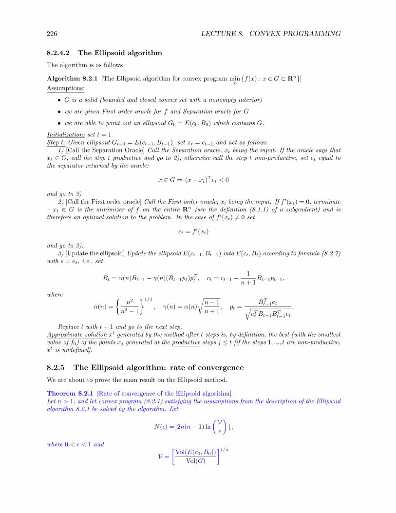
226 LECTURE 8. CONVEX PROGRAMMING
8.2.4.2 The Ellipsoid algorithm
The algorithm is as follows
Algorithm 8.2.1 [The Ellipsoid algorithm for convex program minxf(x) : x ∈ G ⊂ Rn]
Assumptions:
• G is a solid (bounded and closed convex set with a nonempty interior)
• we are given First order oracle for f and Separation oracle for G
• we are able to point out an ellipsoid G0 = E(c0, B0) which contains G.
Initialization: set t = 1Step t: Given ellipsoid Gt−1 = E(ct−1, Bt−1), set xt = ct−1 and act as follows:
1) [Call the Separation Oracle] Call the Separation oracle, xt being the input. If the oracle says thatxt ∈ G, call the step t productive and go to 2), otherwise call the step t non-productive, set et equal tothe separator returned by the oracle:
x ∈ G⇒ (x− xt)T et < 0
and go to 3)2) [Call the First order oracle] Call the First order oracle, xt being the input. If f ′(xt) = 0, terminate
– xt ∈ G is the minimizer of f on the entire Rn (see the definition (8.1.1) of a subgradient) and istherefore an optimal solution to the problem. In the case of f ′(xt) 6= 0 set
et = f ′(xt)
and go to 3).3) [Update the ellipsoid] Update the ellipsoid E(ct−1, Bt−1) into E(ct, Bt) according to formula (8.2.7)
with e = et, i.e., set
Bt = α(n)Bt−1 − γ(n)(Bt−1pt)pTt , ct = ct−1 −
1
n+ 1Bt−1pt−1,
where
α(n) =
n2
n2 − 1
1/4
, γ(n) = α(n)
√n− 1
n+ 1, pt =
BTt−1et√eTt Bt−1BTt−1et
.
Replace t with t+ 1 and go to the next step.Approximate solution xt generated by the method after t steps is, by definition, the best (with the smallestvalue of f0) of the points xj generated at the productive steps j ≤ t [if the steps 1, ..., t are non-productive,xt is undefined].
8.2.5 The Ellipsoid algorithm: rate of convergence
We are about to prove the main result on the Ellipsoid method.
Theorem 8.2.1 [Rate of convergence of the Ellipsoid algorithm]Let n > 1, and let convex program (8.2.1) satisfying the assumptions from the description of the Ellipsoidalgorithm 8.2.1 be solved by the algorithm. Let
N(ε) =c2n(n− 1) ln
(Vε
)b,
where 0 < ε < 1 and
V =
[Vol(E(c0, B0))
Vol(G)
]1/n

8.2. THE ELLIPSOID METHOD 227
Then, for any ε ∈ (0, 1), the approximate solution xN(ε) found by the method in course of the first N(ε)steps, is well-defined and is an ε-solution to the problem, i.e., belongs to G and satisfies the inequality
f(xN(ε))−minG
f ≤ ε[maxG
f −minG
f ]. (8.2.8)
Proof. For the sake of brevity, let N = N(ε). We may assume that the method does not terminate incourse of the first N steps – otherwise there is nothing to prove: the only possibility for the method toterminate is to find an exact optimal solution to the problem.
Let us fix ε′ ∈ (ε, 1), and let x∗ be an optimal solution to (8.2.1) (it exists, since the domain of theproblem is compact and the objective, being convex on Rn, is continuous (we had such a theorem in thecourse Optimization I) and therefore attains its minimum on compact set G.10. Set
G∗ = x∗ + ε′(G− x∗),
so that G∗ is the image of G under homothety transformation with the center at x∗ and the coefficientε′.
By construction, we haveVol(G∗) = (ε′)n Vol(G) > εn Vol(G) (8.2.9)
(“homothety with coefficient α > 0 in Rn multiplies volumes by αn”). On the other hand, by Lemma8.2.1 we have Vol(E(ct, Bt)) ≤ exp−1/(2(n− 1))Vol(E(ct−1, Bt−1)), whence
Vol(E(cN , BN ) ≤ exp− N
2(n− 1)Vol(E(c0, B0)) ≤
[definition of N = N(ε)]≤ V−N εN Vol(E(c0, B0)) =
[definition of V]
=Vol(G)
Vol(E(c0, B0))εN Vol(E(c0, B0)) = εN Vol(G).
Comparing the resulting inequality with (8.2.9), we conclude that Vol(E(cN , BN )) < Vol(G∗), so that
G∗\E(cN , BN ) 6= ∅. (8.2.10)
20. According to (8.2.10), there exists
y ∈ Vol(G∗)\E(cN , BN ).
I claim that
y = (1− ε′)x∗ + ε′z for some z ∈ G; (y − xt)T et > 0 for some t ≤ N (8.2.11)
The first relation in (8.2.11) comes from the inclusion y ∈ G∗: by definition,
G∗ = x∗ + ε′(G− x∗) = x∗ + ε′(z − x∗) | z ∈ G.
To prove the second relation in (8.2.11), note that from the first one y ∈ G ⊂ E(c0, B0), while by theorigin of y we have y 6∈ E(cN , BN ). Consequently, there exists t ≤ N such that
y ∈ E(ct−1, Bt−1) & y 6∈ E(ct, Bt). (8.2.12)
According to our policy of updating the ellipsoids (see Lemma 8.2.1), E(ct, Bt) contains the half-ellipsoid
E+(ct−1, Bt−1) = x ∈ E(ct−1, Bt−1) | (x− xt)T et ≤ 0;
this inclusion and (8.2.12) demonstrate that (y−xt)T et > 0, as required in the second relation in (8.2.11).

228 LECTURE 8. CONVEX PROGRAMMING
30. Now let us look what happens at the step t given by the second relation in (8.2.11). First of all, Iclaim that the step t is productive: xt ∈ G. Indeed, otherwise, by construction of the method, et wouldbe a separator of xt and G:
(x− xt)T et < 0 ∀x ∈ G,
but this relation, as we know from (8.2.11), is violated at y ∈ G and therefore cannot take place.Thus, t is productive, whence, by construction of the method, et = f ′(xt). Now the second relation
in (8.2.11) reads(y − xt)T f ′(xt) > 0,
whence, by definition of subgradient, f(y) > f(xt). This inequality, along with productivity of the stept and the definition of approximate solutions, says that xN is well-defined and
f(xN ) ≤ f(y). (8.2.13)
40. Now we are done. By the first relation in (8.2.11) and due to convexity of f we have
f(y) ≤ (1− ε′)f(x∗) + ε′f(z),
whence
f(y)−minG
f ≡ f(y)− f(x∗) ≤ ε′(f(z)− f(x∗)) ≤ ε′[maxG
f −mingf ] [z ∈ G !];
combining the resulting inequality with (8.2.13), we get
f(xN )−minG
f ≤ ε′[maxG
f −minG
f ].
The latter inequality is valid for all ε′ ∈ (ε, 1), and (8.2.8) follows.
8.2.6 Ellipsoid method for problems with functional constraints
To the moment we spoke about the Ellipsoid method as applied to problem (8.2.1) without functionalconstraints. There is no difficulty to extend the method onto general convex problems (8.0.1). To thisend it suffices to note that (8.0.1) can be immediately rewritten as problem of the type (8.2.1), namely,as
minx
f(x) ≡ f0(x) : x ∈ G ≡ x ∈ G | fi(x) ≤ 0, i = 1, ...,m
. (8.2.14)
All we need to solve this latter problem by the Ellipsoid algorithm is
• to equip (8.2.14) by the Separation and the First order oracles
this is immediate: the First order oracle for (8.2.14) is readily given by the one for (8.0.1). TheSeparation oracle for G can be immediately constructed from the Separation oracle for G and theFirst order oracle for (8.0.1): given x ∈ Rn, we first check whether the point belongs to G, If itis not the case, then it, of course, does not belong to G as well, and the separator (given by theSeparation oracle for G on the input x) separates x from G. Now, if x ∈ G, we can ask the Firstorder oracle about the values and subgradients of f1, ..., fm at x. If all the values are nonpositive,then x ∈ G; if one of this values is positive, then x 6∈ G and, moreover, the vector f ′i(x) (i ≥ 1 is
such that fi(x) > 0) can be used as a separator of x and G (Remark 8.1.1)
• to ensure that G is a solid
(we shall simply assume this).
The resulting algorithm is as follows
Algorithm 8.2.2 [The Ellipsoid algorithm for convex program (8.0.1)]Assumptions:

8.2. THE ELLIPSOID METHOD 229
• G = x ∈ G | fi(x) ≤ 0, i = 1, ...,m is a solid (bounded and closed convex set with a nonemptyinterior)
• we are given First-order oracle for f0, ..., fm and Separation oracle for G
• we are able to point out an ellipsoid G0 = E(c0, B0) which contains G.
Initialization: set t = 1Step t: Given ellipsoid Gt−1 = E(ct−1, Bt−1), set xt = ct−1 and act as follows:
1) [Call the Separation oracle] Call the Separation oracle for G, xt being the input. If the oracle saysthat xt ∈ G, go to 2), otherwise call the step t non-productive, set et equal to the separator returned bythe oracle:
x ∈ G⇒ (x− xt)T et < 0
and go to 4)2) [Call the First order oracle] Call the First order oracle, xt being the input, and check whether
fi(xt) ≤ 0, i = 1, ...,m. If fi(xt) ≤ 0 for all i ≥ 1, call the step t productive and look at f ′0(xt). Iff ′0(xt) = 0, terminate – xt is feasible for (8.0.1) and is the minimizer of f on the entire Rn (see thedefinition (8.1.1) of a subgradient), whence it is an optimal solution to the problem. In the case off ′0(xt) 6= 0 set
et = f ′0(xt)
and go to 4).3) [The case of xt ∈ G and fi(xt) > 0 for some i ≥ 1] Call step t non-productive and find i ≥ 1 such
that fi(xt) > 0 (when we arrive at 3), such an i exists), set
et = f ′i(xt)
and go to 4).4) [Updating the ellipsoid] Update the ellipsoid E(ct−1, Bt−1) into E(ct, Bt) according to formula
(8.2.7) with e = et, i.e., set
Bt = α(n)Bt−1 − γ(n)(Bt−1pt)pTt , ct = ct−1 −
1
n+ 1Bt−1pt−1,
where
α(n) =
n2
n2 − 1
1/4
, γ(n) = α(n)
√n− 1
n+ 1, pt =
BTt−1et√eTt Bt−1BTt−1et
.
Replace t with t+ 1 and go to the next step.Approximate solution xt generated by the method after t steps is, by definition, the best (with the smallestvalue of f) of the points xj generated at the productive steps j ≤ t [if the steps 1, ..., t are non-productive,xt is undefined].
The following result is an immediate corollary of Theorem 8.2.1.
Theorem 8.2.2 [Rate of convergence of the Ellipsoid algorithm on problems with functional constraints]Let n > 1, and let convex program (8.0.1) satisfying the assumptions from the description of the Ellipsoidalgorithm 8.2.2 be solved by the algorithm. Let
N(ε) =c2n(n− 1) ln
(Vε
)b,
where 0 < ε < 1 and
V =
[Vol(E(c0, B0))
Vol(G)
]1/n
Then, for any ε ∈ (0, 1), the approximate solution xN(ε) found by the method in course of the first N(ε)steps, is well-defined and is an ε-solution to the problem, i.e., belongs to G and satisfies the inequality
f(xN(ε))−minG
f ≤ ε[maxG
f −minG
f ]. (8.2.15)

230 LECTURE 8. CONVEX PROGRAMMING
8.3 Ellipsoid method and Complexity of Convex Programming
The Ellipsoid method implies fundamental theoretical results on complexity of Convex Programming; letus briefly discuss these theoretical issues.
8.3.1 Complexity: what is it?
When speaking about complexity of a class of computational problems, we are interested to answer thefollowing crucial question:
Given a family P of problem instances and required accuracy ε, what can be said about the computationaleffort sufficient to solve each instance to the prescribed accuracy?
This is an informal question, of course, and to answer it, we should first formalize the question itself,namely, to say
• What does it mean “a family of problems” and how we measure accuracy of approximate solutions;
• What does it mean “effort of computational process”? What is the model of the process and howthe effort is measured?
To realize that these indeed are points which should be clarified, consider the following “universal solutionmethod” (which in fact is the main method to solve problems): think! Is it a “computational method”?What is the “effort” for this method?
There are basically two approaches to formalize the complexity-related notions. The first, which ismore convenient for “continuous” computational problems, is as follows (according to our goals, I shallspeak only about optimization problems in the form (8.2.1)).
Real Arithmetic Complexity Model:
• A family of problems P is a set of problems (8.2.1) such that a particular member p = (f,G) ofthe family is encoded by a finite-dimensional data vector d(p). The dimension of the data vectoris called the size of the instance.
Example 1. Linear Programming over Reals. Here the instances are of the form
minx
f(x) = cTx : x ∈ G = x ∈ Rn | Ax ≤ b
,
A being m × n matrix and b being m-dimensional vector. The data vector of a problem instanceis comprised of the pair n,m and of n+m+ nm entries of c, b, A written down in a once for everfixed order (e.g., first the n entries of c, then the m entries of b and finally the nm entries of A inthe row-wise order).
Example 2. Quadratically Constrained Quadratic Programming. Here the instances areof the form
minxf0(x) =
1
2xTH0x− bT0 x
subject to
x ∈ G = x ∈ Rn | fi(x) =1
2xTHix− bTi x+ ci ≤ 0, i = 1, ...,m,
and the data vector is comprised of n, m and the entries of the matrices Hi, the vectors bi and thereals ci written down in a once for ever fixed order.
The number of examples can be easily extended; basically, the typical families of problems inquestion are comprised of problems of a “fixed generic analytical structure”, and the data vector isthe set of numerical coefficients of the (fixed by the description of the family) analytical expressionscorresponding to the particular instance in question.
In what follows we restrict ourselves with the families comprised of solvable problems with boundedfeasible sets.

8.3. ELLIPSOID METHOD AND COMPLEXITY OF CONVEX PROGRAMMING 231
• An ε-solution x to a problem instance p = (f,G) is a feasible (x ∈ G) solution such that
f(x)−minG
f ≤ ε[maxG
f −minG
f ];
there are other definitions of an ε-solution, but let us restrict ourselves with the indicated one.
• A computational algorithm for P is a program for an idealized computer capable to perform opera-tions of exact real arithmetic (four arithmetic operations and computation of elementary functionslike√·, sin(·), log(·), etc.). When solving a problem instance from P, the algorithm gets on
input the data vector of the instance and the required accuracy ε and starts to process thesedata; after finitely many elementary steps the algorithm should terminate and return the vec-tor xout of the corresponding dimension, which should be an ε-solution to the input instance.The computational effort of solving the instance is, by definition, the total # of elementary steps(arithmetic operations) performed in course of processing the instance.
The second way to formalize the complexity-related notions, the way which is the most widely usedin theoretical Computer Science and in Combinatorial Optimization, is given by
Algorithmic Complexity Model:
• A family of problems is a set of problems (8.2.1) such that a particular member p = (f,G) of thefamily is encoded by an integer i(p); the # L of digits in this integer is the bit size of the instancep.
Example 3. Integer programming. Here the problem instances are of the form
minx
f(x) = cTx : x ∈ G = x ∈ Zn | Ax ≤ b
,
where Zn is the space of n-dimensional vectors with integer entries, c and b are vectors of dimensionsn and m with integer entries, and A is an m× n matrix with integer entries.
To encode the data (which form a collection of integers) as a single integer, one can act as follows:
first, write down the data as a finite sequence of binary integers (similarly to Example 1, wherethe data were real);
second, encode the resulting sequence of binary integers as a single integer, e.g., by representing
- binary digit 0 as 00
- binary digit 1 as 11
- blank between integers as 01
- sign – at an integer as 10
Example 4. Linear Programming over Rationals. This is a subfamily of the Linear Pro-gramming family (Example 1), where we impose on all the entries of c, b, A the requirement to berational numbers. To encode a problem instance by a single binary integer, it suffices to write thedata as a sequence of binary integers, same as in Example 3 (with the only difference that nowevery rational element of the data is represented by two sequential integers, its numerator anddenominator), and then encode the sequence, as it was explained above, by a single binary integer.
In what follows, speaking about Algorithmic Complexity model, we always assume that
- the families in question are comprised of solvable problems with bounded feasible sets
- any problem instance from the family admits a solution which can be naturally encoded by abinary integer
The second assumption is clearly valid for the Integer Programming (Example 3). It is also validfor Linear Programming over Rationals (Example 4), since it can be easily proved that a solvableLP program with integer data admits a solution with rational entries; and we already know thatany finite sequence of integers/rationals can be naturally encoded by a single integer.

232 LECTURE 8. CONVEX PROGRAMMING
• Normally, in Algorithmic Complexity model people are not interested in approximate solutions andspeak only about exact ones; consequently, no problem with measuring accuracy occurs.
• A computational algorithm is an algorithm in any of (the equivalent to each other) definitions givenin Mathematical Logic; you loose nothing when thinking of a program for an idealized computerwhich is capable to store in memory as many finite binary words as you need and to performbit-wise operations with these words. The algorithm as applied to a problem instance p from Pgets on input the code i(p) of the instance and starts to process it; after finitely many elementarysteps, the algorithm should terminate and return the code of an exact solution to the instance.The computational effort is measured as the total # of elementary bit-wise operations performedin course of the solution process.
Let me stress the difference between the notions of the size of an instance in the Real Arithmeticand the Algorithmic Complexity models. In the first model, the size of an instance is, basically, the #of real coefficients in the natural analytical representation of the instance, and the size is independent ofthe numerical values of these coefficients – they may be arbitrary reals. For example the Real Arithmeticsize of any LP program over Reals (Example 1) with n = 2 variables and m = 3 inequality constraints isthe dimension of the vector
(2, 3, c1, c2, b1, b2, b3, A11, A12, A21, A22, A31, A32),
i.e., 13. In contrast to this, the Algorithmic Complexity size of an LP program over Rationals (Example4) with n = 2 variables and m = 3 constraints can be arbitrarily large, if the rational data are “long”.
We can observe similar difference between the measures of computational effort in the Real Arithmeticand the Algorithmic Complexity models. In the first of them, the effort required, say, to add two reals isone, independently of what the reals are. In the second model, we in principle cannot deal with reals –only with integers; and the effort to add two N -digit integers is not 1 – it is proportional to N .
8.3.2 Computational Tractability = Polynomial Solvability
After the main complexity-related notions – family of problems, ε-solution, solution algorithm and itscomputational effort – are formalized, we may ask ourselves
What is the complexity of a given family of problems, i.e., the best possible, over all solution algorithms,computational effort sufficient to solve all instances of a given size to a given accuracy?
Before trying to answer this question, we may ask ourselves a more rough (and, in a sense, more important)question:
Is the family in question computationally tractable, i.e. is its complexity a “reasonable” function of thesize of instances?
If the answer to this second question is negative, then we may forget about the first one: if we know thatto solve an instance of size l from a family P it may require at least 2l elementary steps, then we may
not bother much whether the actual complexity is 2l, 25l or 2(2l): in the first case, the maximal size ofinstances we are able to solve for sure in reasonable time is something like 30, in the second – 6, in thethird – 5; this difference normally means nothing, since the sizes of actually interesting problems usuallyare hundreds, thousands and tens of thousands.
Now, the notion of “computationally tractable” complexity in theoretical studies of the last 30 yearsis unanimously understood as the one of “polynomial time” solvability. This latter notion first wasintroduced in the Algorithmic Complexity model and was defined as follows:
A solution algorithm A for a family P of problem instances is called polynomial, if the computationaleffort required by A to solve a problem instance of an arbitrary bit size L never exceeds q(L), q beingcertain polynomial; here all complexity-related notions are understood according to the AlgorithmicComplexity model.P is called polynomially solvable, if it admits polynomial solution algorithm.

8.3. ELLIPSOID METHOD AND COMPLEXITY OF CONVEX PROGRAMMING 233
The analogy of this definition for the Real Arithmetic Complexity model is as follows:
A solution algorithms A for a family P of problem instances is called R-polynomial, if the computationaleffort required by A to solve a problem instance p of an arbitrary size l to an arbitrary accuracy ε ∈ (0, 1)never exceeds
q(l) ln
(V(p)
ε
), (8.3.1)
where q is certain polynomial and V(p) is certain data-dependent quantity; here all complexity-relatednotions are understood according to the Real Arithmetic Complexity model.
The definition of an R-polynomial algorithm admits a very natural interpretation. The quantityln(V(p)/ε) can be viewed as # of accuracy digits in an ε-solution; with this interpretation, (8.3.1) meansthat the arithmetic cost per accuracy digit is bounded from above by a polynomial of the dimension ofthe data vector.
8.3.3 R-Polynomial Solvability of Convex Programming
Invention of the Ellipsoid method (1976) allowed to establish the following important
Theorem 8.3.1 [R-polynomial solvability of Convex Programming]Consider a family P of convex problems (8.2.1) and assume that
(i) all problem instances p = (f,G) from the family are bounded (i.e., their feasible domains G arebounded) and strictly feasible (i.e., their feasible domains G possess nonempty interiors); moreover, giventhe data vector d(p) of the instance, one can in polynomial in the size lp = dim d(p) of the instancenumber of arithmetic operations compute an ellipsoid which covers G along with a lower bound vp > 0for the volume of G;
(ii) given an instance p = (f,G) ∈ P and a point x ∈ Rnp , np being the # of variables in p, on canin polynomial in lp number of arithmetic operations
• imitate the Separation oracle for G on the input x, i.e., check the inclusion x ∈ G and, if it is notvalid, compute a separator e:
supy∈G
eT y < eTx;
• imitate the First order oracle for f , i.e., compute f(x) and f ′(x).
Then there exists an R-polynomial algorithm for P.
Proof is immediate: it suffices to use the Ellipsoid algorithm. Indeed,
• (i) says that, given on input the data vector d(p) of a problem instance p ∈ P, we can in polynomialin lp = dim d(p) number of arithmetic operations compute an ellipsoid E(c0, B0) and thus start theEllipsoid algorithm. As a byproduct, we observe that the number of variables np in p is boundedfrom above by a polynomial of the size lp of the instance (otherwise it would require too manyoperations simply to write down the center of the ellipsoid).
• according to the description of the method, to perform a step of it, we should imitate the Separationand, possibly, the First order oracle at current point xt (according to (iii), it takes polynomial in lpnumber of arithmetic operations) and then should perform O(n2
p) arithmetic operations to updatethe previous ellipsoid into the current one according to Algorithm 8.2.1.3); by virtue of the previousremark, np is bounded from above by a polynomial in lp, so that the overall arithmetic effort at astep is polynomial in lp;
• according to Theorem 8.2.1, the method will find an ε-solution to p in the number of steps notexceeding
N(ε) =c2(np − 1)np ln
(Vε
)b, V =
[Vol(E(c0, B0))
Vol(G)
]1/np
;

234 LECTURE 8. CONVEX PROGRAMMING
we have
N(ε) ≤ N ′(ε) =c2(np − 1)np ln
(Vol1/np(E(c0, B0))
v1/npp ε
)b
(see (i)); according to (i), we can compute N ′(ε) in polynomial in lp number of operations andterminate the process after N ′(p) steps, thus getting an ε-solution to p.
The overall arithmetic effort to find an ε-solution to p, in view of the above remarks, is bounded fromabove by
r(lp)N′(ε) ≤ q(lp) ln
(V(p)
ε
), V(p) ≡
[Vol(E(c0, B0))
vp
]1/np
,
both r(·) and q(·) being certain polynomials, so that the presented method indeed is R-polynomial.When thinking of Theorem 8.3.1, you should take into account that the “unpleasant” assumptions
(i) are completely technical and normally can be ensured by slight regularization of problem instances.Assumption (ii) is satisfied in all “non-pathological” applications, so that in fact Theorem 8.3.1 can bequalified as a General Theorem on R-Polynomial Solvability of Convex Programming. I should add thatthis is, in a sense, an “existence theorem”: it claims that in Convex Programming there exists a “universal”R-polynomial solution routine, but it does not say that this is the best possible R-polynomial routine forall particular cases. The main practical drawback of the Ellipsoid method is that it is “slow” – the # ofiterations required to solve the problem within a once for ever fixed accuracy ε grows quadratically withthe dimension n of the problem. This quadratic in n growth of the effort makes it basically impossibleto use the method as a practical tool in dimensions like hundreds and thousands. Recently, for manyimportant families of Convex Programming problems (Linear, Quadratically Constrained Quadratic,Geometric and some others) more specialized and more efficient interior point polynomial algorithmswere developed; these methods are capable to struggle with large-scale problems of real-world origin.
I would say that the Ellipsoid method, as a practical tool, is fine for not large – up to 20-30 variables– convex problems. The advantages of the method are:
• simplicity in implementation and good numerical stability
• universality
• low order of dependence of computational effort on m – the # of functional constraints
The latter remark relates to Algorithm 8.2.2): the number of steps required to achieve a givenaccuracy is simply independent of m, and the effort per step is at most proportional to the m (theonly place where the number of constraints influence the effort is the necessity to check feasibility ofthe current iterate and to point out a violated constraint, if any exists). As a result, for “high andnarrow” convex programs (say, with up to 20-30 variables and as many thousands of constraints asyou wish) the Ellipsoid method seems to be one of the best known Convex Programming routines.
8.4 Polynomial solvability of Linear Programming
Surprisingly, the most important “complexity consequences” of the Ellipsoid method – which is a purely“continuous optimization” algorithm – relate to Algorithmic Complexity. The most known of theseconsequences is
8.4.1 Polynomial Solvability of Linear Programming over Rationals
8.4.1.1 Some History
Everybody knows that Linear Programming programs – both with real and rational data – can be solvedefficiently (and are solved almost for 50 years) by the Simplex Algorithm, which is a finite Real Arithmeticroutine for LP capable to solve huge practical linear programs. What I am not sure is that everybody

8.4. POLYNOMIAL SOLVABILITY OF LINEAR PROGRAMMING 235
knows what does it mean “efficiently” in the above sentence. This is practical efficiency – when solvingan LP program
minx
cTx : Ax ≤ b
(8.4.1)
with n variables and m > n inequality constraints, the Simplex normally performs 2m - 4m iterationsto find the solution. Anyhow, theoretically Simplex is not a polynomial algorithm: since the beginningof sixties, it is known that there exist simple LP programs pn with n = 1, 2, 3, ... variables and integerdata of the total bit size Ln = O(n2) such that some versions of the Simplex method solve pn in no lessthan 2n steps. Consequently, the aforementioned versions of the Simplex method are not polynomial –for a polynomial algorithm, the solution time should be bounded by a polynomial of Ln = O(n), i.e.,of n. Similar “bad examples” were constructed for other versions of the Simplex method; and althoughnobody was able to prove that no version of Simplex can be polynomial, nobody was also lucky to pointout a polynomial version of the Simplex method. Moreover, since mid-sixties, where the AlgorithmicComplexity approach became standard, and till 1979 nobody knew whether LP over Rationals (Example4 above) is or is not polynomially solvable.
8.4.2 Khachiyan’s Theorem
The positive answer on the fundamental question whether LP over Rationals is polynomially solvable wasgiven only in 1979 by L. Khachiyan; the main tool used in the proof was the Ellipsoid method invented3 years earlier.
Below I sketch the reasoning of Khachiyan.
8.4.2.1 Step 1: from Optimization to Feasibility
The first step of the construction reduces the optimization LP program (8.4.1) to the Feasibility programfor a system of linear inequalities. To this end it suffices to write down both the inequalities of (8.4.1)and of its LP dual and to replace minimization in the primal problem and maximization in the dual onewith the linear constraint that the duality gap should be zero. This results in the following system oflinear inequalities and equations:
Ax ≤ b; AT y = c; y ≤ 0; cTx = bT y (8.4.2)
with unknowns x ∈ Rn and y ∈ Rm. The Duality Theorem in Linear Programming says that the originalproblem (8.4.1) is solvable if and only if (8.4.2) is, and if it is the case, then x-components of the solutionsto (8.4.2) are exactly the optimal solutions to (8.4.1).
Assembling x and y in a single vector of variables u, representing u as the difference of new nonnegativevariable vectors v and w and, finally, assembling v and w into single vector z (all these manipulations arestandard tricks in LP),
we can rewrite (8.4.2) equivalently as the problem
find z ∈ RN : Qz ≤ q, z ≥ 0; (8.4.3)
here N = 2(n + m), and Q, q are certain matrix and vector with rational entries coming, in an evidentfashion, from the initial data c, b, A. Note that the bit size L1 of the data in (8.4.3) is of order of the bitsize L of the initial data in (8.4.1); in fact L1 ≤ 10L.
It is convenient to pass from problem (8.4.3) with rational data to an equivalent problem with integerdata; to this end it suffices to compute the common denominator of all the fractions involved into (8.4.3)and to multiply all the data by this common denominator. As a result, we come to the problem
find x ∈ RN : Rz ≤ r, z ≥ 0; (8.4.4)
the properties of this problem are as follows:
• (8.4.3) is equivalent to the LP program (8.4.1): both the problems are solvable/unsolvable simul-taneously; if they are solvable, then any solution to (8.4.4) can be converted in an explicit andsimple manner into optimal solution to (8.4.1);

236 LECTURE 8. CONVEX PROGRAMMING
• the data in (8.4.4) are integer, and their bit size L2 is bounded by a polynomial (something like200L2) of the bit size L of the initial data 4).
It follows that if we were able to solve in polynomial time the Feasibility problem (8.4.4), we would get,as a byproduct, a polynomial algorithm for the initial problem (8.4.1).
8.4.2.2 Step 2: from Feasibility to Solvability
Instead of attacking the Feasibility problem (8.4.4) (where we are asked to check whether (8.4.4) issolvable and if it is the case – are asked to point out a solution), let us for the time being restrict ourgoals with the following relaxed solvability version of (8.4.4):
(S) given the data of (8.4.4), detect whether the problem is solvable.
The simplification, as compared to (8.4.4), is that now we are not obliged to point out an explicit solutionto a solvable instance.
Problem (S) is the problem which is solved in polynomial time by the Ellipsoid method. This is doneas follows.
• From (S) to (S′). Problem (S) clearly is equivalent to the following optimization problem: let
f(z) = max [(Rz)1 − r1|; (Rz)2 − r2; ...; (Rz)M − rM |]
(M is the number of rows in R) be the residual function of the system of inequalities Rz ≤ r; thisfunction clearly is nonnegative at a nonnegative z if and only if z is a feasible solution to (8.4.4).Consequently, (S) is exactly the following problem:
(S′): detect whether minz∈RN ,z≥0
f(z) ≤ 0
((S) is solvable if and only if the answer in (S′) is “yes”).
• From (S′) to (S′′). The next step is given by the following simple
Lemma 8.4.1 The answer in (S′) is “yes” if and only if it is “yes” in the following problem
(S′′) detect whether minz:0≤zi≤2L2 , i=1,...,N
f(z) ≤ 0
L2 being the bit length of the data in (S).
Proof. If the answer in (S′′) is “yes”, then, of course, the answer in (S′) also is “yes”. It remainsto prove, therefore, that if the answer in (S′) is “yes” (or, which is the same, if (S) is solvable),then the answer in (S′′) also is “yes”. This is easy. The solution set of (S), being nonempty, is anonempty closed convex polyhedral set (here and in what follows I use the standard terminologyof Convex Analysis; this terminology, along with all required facts, was presented in the courseOptimization I); since (S) involves nonnegativity constraints, this set does not contain lines, andtherefore, due to the well-known fact of Convex Analysis, possesses an extreme point z. From thestandard facts on the structure of extreme points of a polyhedral set given by (8.4.4) it is knownthat the vector z∗ comprised of nonzero entries of z, if such entries exist, satisfy nonsingular systemof linear equations of the form
Rz∗ = r,
where
4the latter property comes from the fact that the common denominator of the entries in (8.4.3) is an integerof bit size at most L1 ≤ 10L; therefore when passing from (8.4.3) to (8.4.4), we increase the bit size of each entryby at most 10L. Since even the total bit size of the entries in (8.4.3) is at most 10L, the bit size of an entry in(8.4.4) is at most 20L; and there are at most 10L entries. All our estimates are extremely rough, but it does notmatter – all we are interested in is to ensure polynomiality of the bit size of the transformed problem in the bitsize of the initial one

8.4. POLYNOMIAL SOLVABILITY OF LINEAR PROGRAMMING 237
– R is a k × k nonsingular submatrix in R (k is the # of nonzero entries in z)
– r is certain fragment of the right hand side vector r
(R and r are given by (8.4.4)).
It follows that the entries in z∗ are given by the Cramer rules – they are ratios of certain k × kdeterminants taken from the k × (k + 1) matrix [R|r]:
z∗i =∆i
∆0.
All entries in this matrix are integers, and the total bit size of the entries does not exceed L2. Itfollows that all the determinants are, in absolute value, at most 2L2 5). Thus, the numerators inthe Cramer formulae are ≤ L2 in absolute values, while the denominator (being a nonzero integer)is in absolute value ≥ 1. Consequently, |z∗i | ≤ 2L2 .
Thus, all nonzero entries in z are ≤ 2L2 in absolute values. Since z is a solution to (S), this isa point where f is nonnegative. We conclude that if the answer in (S) is “yes”, then f attainsnonpositive value in the box 0 ≤ zi ≤ 2L2 , 1 ≤ i ≤ N , so that the answer in (S′′) also is “yes”.
• (S′′) as a convex program. To solve problem (S′′) is exactly the same as to check whether theoptimal value in the optimization program
minx
f(z) : z ∈ G = z ∈ Rn | 0 ≤ zi ≤ 2L2 , i = 1, ..., N
(8.4.5)
is or is not positive. The objective in the problem is easily computable convex function (sinceit is maximum of M linear forms), and the domain G of the problem is a simple solid - a box.Remark 8.1.1 explains how to imitate the First order and the Separation oracles for the problem;we can immediately point out the initial ellipsoid which contains G (simply the Euclidean ballcircumscribed around the cube G). Thus, we are able to solve the problem by the Ellipsoidmethod. From Theorem 8.2.1 (where one should estimate the quantities V and max
Gf −min
Gf via
L2; this is quite straightforward) it follows that in order to approximate the optimal value f∗ in(8.4.5) within a prescribed absolute accuracy ν > 0, it suffices to perform
Nν = O(1)N2[L2 + ln1
ν]
steps with at most O(1)(M +N)N arithmetic operations per step, which gives totally
M(ν) = O(1)N3(M +N)[L2 + ln1
ν] (8.4.6)
arithmetic operations (O(1) here and in what follows are positive absolute constants).
All this looks fine, but in order to detect whether the optimal value f∗ in (8.4.5) is or is not non-positive (i.e., whether (S) is or is not solvable), we should distinguish between two “infinitesimallyclose to each other” hypotheses f∗ ≤ 0 and f∗ > 0, which seems to require the exact value of f∗;
5This is a consequence of the Hadamard inequality: the absolute value of a determinant (≡ the volume of theparallelotope spanned by the rows of the determinant) does not exceed the product of the Euclidean lengths ofthe rows of the determinant (product of the edges of the parallelotope). Consequently, log2|∆i| does not exceedthe sum of binary logs of the Euclidean lengths of the rows of [R|r]. It remains to note that the binary logarithmof the Euclidean length of an integer vector clearly does not exceed the total bit length of the vector:
1
2log2(a2
1 + ...+ a2k) ≤ 1
2log2[(1 + a2
1)(1 + a2)2...(1 + a2k)] =
k∑i=1
1
2log2[1 + a2
i ] ≤k∑i=1
log2[1 + |ai|]
and the latter expression clearly is ≤ the total # of binary digits in integers a1, ..., ak.

238 LECTURE 8. CONVEX PROGRAMMING
and all we can do is to approximate “quickly” f∗ to a prescribed accuracy ν > 0, not to find f∗
exactly.
Fortunately, our two hypotheses are not infinitesimally close to each other – there is a “gap”between them. Namely, it can be proved that
if the optimal value f∗ in (8.4.5) is positive, it is not too small, namely f∗ ≥ 2−π(L2) with certainpolynomial π(·) 6).
The latter remark says that to distinguish between the cases f∗ ≤ 0 and f∗ > 0 means in fact todistinguish between f∗ ≤ 0 and f∗ ≥ 2−π(L2); and to this end it suffices to restore f∗ within absoluteaccuracy like ν = 2−π(L2)−2. According to (8.4.6), this requires O(1)N3(N + M)[L2 + π(L2)]arithmetic operations, which is not more than a polynomial of L2 and, consequently, of L (sinceL2 is bounded from above by a polynomial of L).
Thus, we indeed can decide whether f∗ is or is not nonpositive or, which is the same, whether (S)is or is not solvable, in polynomial in L number of arithmetic operations.
This is not exactly what we need: our complexity model counts not arithmetic, but bit-wiseoperations. It turns out, anyhow (the verification is straightforward, although very dull), that onecan apply the Ellipsoid method with inexact arithmetic instead of the exact one, rounding theintermediate results to a polynomial in L number of accuracy digits, and it still allows to restoref∗ within required accuracy. With the resulting inexact computations, the bit-wise overall effortbecomes polynomial in L, and the method becomes polynomial.
Thus, (S) is polynomially solvable.
8.4.2.3 From Solvability back to Feasibility
It remains to explain how, given possibility to solve in polynomial time the Solvability problem (S), onecould solve in polynomial time the Feasibility problem (8.4.4) and thus – the original problem (8.4.1).
First of all, we solve (S) – we already know how to do it in polynomial time. If the answer in (S) is“no”, then (8.4.4) is unsolvable, and we are done. It remains to consider the case when the answer in (S)is “yes”; here we should point out explicitly the solution to the system
(*0): Pz ≤ p, z ≥ 0.
Let us act as follows. Take the first inequality PT1 z ≤ p1 in the system Pz ≤ p and make it equality.This will give us a new system (*+
1 ) of, basically, the same bit size. as the one of (*0). Let us check inpolynomial time whether this new system is solvable. If it is so, let (*1) be the system obtained from(*0) by replacing the first inequality with the equality; note that this system is solvable, and all solutionsto it are solutions to (*0). If (*+
0 ) is unsolvable, it means that the hyperplane Π = PT1 z = p1 does notintersect the solution set of (*0). Since the latter set is nonempty and convex, the only possibility forthe hyperplane Π not to intersect this set is when the inequality PT1 z ≤ p1 is redundant in system (*0)– when eliminating this inequality from the system, we do not vary the solution set. If it is the case, letus define (*1) as the system obtained from (*0) by eliminating the first inequality.
Let us look what we get. Solving in polynomial time problem (S) associated with the system (*+1 )
with basically the same bit size as the one of (8.4.4), we have updated the initial system of inequalities
6The proof (I skip the details) is completely similar to that one of Lemma 8.4.1: we again exploit the fact thatf∗ is the optimal value in certain LP program with integer data of the polynomial in L2 total bit size, namely, inthe program
mint,z
t : t ≥ (Pz)i − pi, i = 1, ..., N, 0 ≤ zi ≤ 2L2
.
The optimal value in this problem is achieved at an extreme point, and this point, same as in Lemma 8.4.1, isrational with not too large numerators and denominators of the entries. Consequently, the optimal value of t isrational with not too large numerator and denominator, and such a fraction, if positive, of course, is not too closeto 0.
8.4. POLYNOMIAL SOLVABILITY OF LINEAR PROGRAMMING 239
(*0) into a new system (*1); this new system is solvable, and every solution to it is a solution to (*0) aswell, and the new system has one inequality less than the initial system.
Now let us apply the same trick to system (*1), trying to make the equality the second inequalityPT2 z ≤ p2 of the initial system; as a result, we will “kill” this second inequality – either make it theequality, or eliminate it at all – and all solutions to the resulting system (*2) (which for sure will besolvable) will be solutions to (*1) and, consequently, to the initial system (*0).
Proceeding in this manner, we in M steps (M is the row size of P ) will “kill” all the inequalitiesPz ≤ p - some of them will be eliminated, and some - transformed into equalities. Now let us kill inthe same fashion the inequalities zi ≥ 0, i = 1, ..., N . As a result, in N more steps we shall “kill” allinequalities in the original system (*0), including the nonnegativity ones, and shall end up with a systemof linear equations. According to our construction, the resulting system (*M+N ) will be solvable andevery solution to it will be a solution to (*0).
It follows that to get a solution to (*0) it remains to solve the resulting solvable system (*M+N ) oflinear equations by any standard Linear Algebra routine (all these routines are polynomial).
Note that the overall process requires to solve N +M Solvability problems of, basically, the same bitsize as (8.4.4) and to solve a system of linear equations, again of the same bit size as (8.4.4); thus, theoverall complexity is polynomial in the size of (8.4.4).
The proof of polynomial time solvability of LP over Rationals – which might look long and dull – infact uses absolutely simple and standard arguments; the only nonstandard – and the key one – argumentis the Ellipsoid method.
8.4.3 More History
Although the Ellipsoid method as applied to LP turns out to be polynomial – and therefore, theoretically,much more efficient than the non-polynomial Simplex method – in practical computations the Simplex(which – it is a kind of mystery why – never works according to its disastrous theoretical worst caseefficiency bound) is incredibly better than the Ellipsoid method, so that it makes absolutely no sense tothink that the Ellipsoid method can be competitive with Simplex as a practical LP tool. Nevertheless,the “complexity approach” to LP proved itself to be fruitful not only in theory. In 1984, N. Karmarkardeveloped a new polynomial time algorithm for LP – the first of the interior point methods which arein great fashion now – and this method turned out to be quite competitive with the Simplex method inpractical computations, not speaking about great theoretical advantage of polynomiality shared by themethod of Karmarkar.

240 LECTURE 8. CONVEX PROGRAMMING

Lecture 9
Active Set and Penalty/BarrierMethods
The traditional methods for general type constrained minimization problems
(P )f(x) → min
s.t.hi(x) = 0, i = 1, ...,m,gj(x) < 0, j = 1, ..., k
with x ∈ Rn (when saying “general type problems”, I mean not necessarily convex ones; Convex Pro-gramming is another and much nicer story) can be, roughly speaking, separated into the following fourgroups:
• primal methods, where we try to act similarly to what we did in the unconstrained case – i.e., tomove along the feasible set in a way which ensures, at each step, progress in the objective;
• barrier and penalty methods, where we reduce (P ) to a series of “approximating” the problemunconstrained programs;
• Lagrange multipliers methods, where we focus on the dual problem associated with (P ); this dualproblem is either unconstrained one (when (P ) is equality constrained), or has simple nonnegativityconstraints (when (P ) includes inequalities) and is therefore simpler than (P ). When solving thedual problem, we get, as a byproduct, approximate solutions to (P ) itself. Note that a posteriori theLagrange multiplier methods, same as the penalty/barrier ones, reduce (P ) to a sequence of uncon-strained problems, but in a “smart” manner quite different from the straightforward penalty/barrierscheme;
• SQP (Sequential Quadratic Programming) methods. The SQP methods, in contrast to all previousones, neither try to improve the objective staying within the feasible set, nor approximate theconstrained problem by unconstrained ones, but directly solve the KKT system of (nonlinear)equations associated with (P ) by a kind of the Newton method.
This lecture is devoted to brief overview of the first two groups of methods; my choice is motivatedby the fact that these methods basically directly reduce the constrained problem to a sequence of un-constrained ones, and it is easy to understand them, given our knowledge of technique for unconstrainedminimization.
Before passing to the main body of the lecture, let me make an important comment.
When solving an unconstrained minimization problem, we were aimed to find the optimalsolution; but the best we indeed were able to do was to ensure convergence to the set ofcritical points of the objective, the set of points where the First Order Necessary Optimality
241

242 LECTURE 9. ACTIVE SET AND PENALTY/BARRIER METHODS
condition – the Fermat rule – is satisfied. Similarly, the best we can do in constrainedoptimization is to ensure convergence to the set of KKT points of the problem – those pointswhere the First Order Necessary Optimality condition form Lecture 7 is satisfied. Whetherit fits our actual goal or not – this is another story, sometimes with happy end (e.g., in thecase of convex problem a KKT point is for sure a globally optimal solution), sometimes –not, but this is all we can achieve.
During all this lecture, we make the following assumption on problem (P ) in question:
Regularity: The problem is regular, i.e., it is feasible, the objective and the constraints are at least oncecontinuously differentiable, and every feasible solution x is a regular point for the system of constraints:the gradients of the constraints active at x (i.e., satisfied at x as equalities) are linearly independent.
9.1 Primal methods
Just to start our considerations, let me briefly outline the idea of the oldest primal method – the FeasibleDirections one.
9.1.1 Methods of Feasible Directions
The Feasible Directions method can be applied only to a problem without nonlinear equality constraints.To simplify considerations, assume that all our constraints are linear inequalities, so that the problem is
(LIP) minx
f(x) : gj(x) ≡ aTj x− bj ≤ 0, j = 1, ...,m
. [x ∈ Rn] (9.1.1)
The idea of the method is as follows: the First Order Necessary Optimality conditions (the KKT condi-tions) are “constructive”: if they are not satisfied at a given feasible solution x, then we can explicitlypoint out a better – with a smaller value of the objective – feasible solution x+.
Indeed, we remember from the Lecture 7 that the KKT conditions were obtained from the followingconstruction: given feasible solution x, we associate with it linearization of (LIP) at x – the auxiliaryLinear Programming program
(LIPx) minxf(y) ≡ f(x) + (y − x)T∇f(x)
subject to
gj(y) ≤ 0, j = 1, ...,m.
x is a KKT point of (9.1.1) if and only if x is optimal solution to (Px) (this was exactly the conjecturewhich led us to the KKT condition).
From this “if and only if” statement we conclude that if x is not a KKT point of (9.1.1), then x isnot optimal solution to (Px). In other words (pass in (Px) from variable y to d = y − x), there exists adescent direction d – direction satisfying
dT∇f(x) < 0, gj(x+ d) ≤ 0, j = 1, ...,m.
When performing a small enough step in this direction, we improve the objective (by the same reasonsas in the Gradient Descent) and do not violate the constraints; after such a step is performed, we caniterate the construction at the new point, an so on.
Normally, at a non-KKT point there exist many descent directions. In the Feasible Directions methodwe choose the one which is “most perspective” – along which the objective decreases at the highest possiblerate. Of course, to choose the most perspective direction, we should normalize somehow the candidates.The standard normalization here is given by the restriction
|di| ≤ 1, i = 1, ..., n, (9.1.2)

9.1. PRIMAL METHODS 243
so that the direction in question is the solution to the following LP program:
mind
dT∇f(x) : gj(x+ d) ≤ 0, j = 1, ...,m, |di| ≤ 1, i = 1, ..., n
. (9.1.3)
Normalization (9.1.2) instead of more natural normalization like |d| ≤ 1 is motivated by the desire forthe direction to be determined via an LP, and thus effectively solvable, program.
After the “most perspective” direction d is found, we define the largest stepsize γ, let it be called γ,among the stepsizes which keep the point x+γd feasible, and define the next iterate x+ via the linesearchapplied to f on the segment [0, γ]:
x+ ∈ Argminf(y) : y = x+ γd, 0 ≤ γ ≤ γ.
Then we replace x with x+ and loop.The outlined idea can be naturally extended onto inequality constrained problems with nonlinear
constraints, but we are not going to discuss this issue in more details. What should be said is thatFeasible Directions methods almost never are used in practice – too often they turn out to be tooslow, even in “good” – linearly constrained – situations. Much better methods for linearly constrainedoptimization are Active Set methods which we are about to consider.
9.1.2 Active Set Methods
Consider a linearly constrained problem (P ) – one with linear inequality and equality constraints, and letG be the feasible domain of the problem. For the sake of convenience, assume that there are no equalityconstraints at all – we always can make it the case replacing the entire Rn by the affine set given by theequality constraints.
The feasible domain G of the problem is given by finite set of linear inequalities, so that it is apolyhedral set. We may classify all feasible solutions to the problem – all points of G – according towhich constraints are active at these solutions, so that an arbitrary subset I of the set I = 1, ...,mof constraint indices defines a “face” GI in G; GI is comprised of all feasible solutions x such that theconstraints gi with indices from I are active at x (when I is empty, then, by definition, GI is the entireG). For some I, the faces SI can be empty; from now on, we shall not be interested in these “emptyfaces” and will call faces only those of the sets GI which are nonempty. For each face GI , let SI be affineset given by the system of linear equalities
gi(x) = 0, i ∈ I,
so that GI is a polyhedral set in SI ; to get this set, we should add to the linear equalities defining SIlinear inequalities
gi(x) ≤ 0, i 6∈ I.From the Regularity assumption it follows that a face GI is a polyhedral set of affine dimension exactlyn−Card(I), where Card(I) is the number of elements in the set I, and that affine dimension of the affineset SI also is n−Card(I); in other words, SI is the affine span of GI . G∅ – the only face of affine dimensionn - is the entire G; the boundary of G is comprised of facets – (n − 1)-dimensional polyhedral sets GIassociated with one-element sets I. The relative boundary of a facet is comprised of (n− 2)-dimensionalfaces GI corresponding to 2-element sets I, and so on, until we come to 1-dimensional edges – faces GIassociated with (n−2)-element sets I – and vertices – faces of dimension 0 given by n-element sets I. Thesimplest way to get an impression of this face structure of G is to imagine a 3D cube given by 6 linearinequalities xi − 1 ≤ 0, −1− x1 ≤ 0, i = 1, 2, 3. Here we have one 3-dimensional facet – the entire cube;it is bounded by 6 2-dimensional facets, each of them being bounded by 4 1-dimensional edges (there aretotally 12 of them). And edges, in turn, are bounded by 0-dimensional vertices (totally 8).
9.1.2.1 Active Set scheme: the idea
Now let us look at our optimization problem, where we should minimize a smooth objective over G. Justto explain the idea of the active set methods, assume for a moment that the objective is strongly convex,

244 LECTURE 9. ACTIVE SET AND PENALTY/BARRIER METHODS
so that there is exactly one KKT point x∗ in our problem, which is the global solution. Let us denote byI∗ the set of indices of those constraints which are active at x∗; then x∗ belongs to the relative interior ofthe face GI∗ (the constraints active at x∗ participate in the description of the affine span SI∗ of GI∗ , andthe remaining constraints are satisfied at x∗ as strict inequalities). Since x∗ is globally optimal solutionto our problem, it is also optimal solution to the problem
minxf(x) : x ∈ GI∗ ,
(since the feasible set of the latter problem contains x∗ and is contained in G), and since x∗ is a relativeinterior point of GI∗ , it is a local solution to the problem
(PI∗) minxf(x) : x ∈ SI∗ .
But the objective f is strongly convex, so that x∗ is a local solution to the latter problem if and onlyif it is a global solution to it, and such a solution is unique. It follows that if we were clever enough toguess in advance what is I∗, we could solve instead of our original problem (P ) the problem (PI∗). Now,the problem (PI∗) is actually unconstrained – we could choose orthogonal coordinates in the affine setSI∗ , express the n original coordinates of a point x ∈ SI∗ as linear functions of these new coordinatesand substitute these expressions into f , thus getting a function f of k = dim SI∗ new coordinates – therestriction of f onto SI∗ . Problem (PI∗) clearly is equivalent to unconstrained minimization of f , so thatit can be solved via unconstrained minimization machinery already known to us1).
We see that if we were clever enough to guess what are the constraints active at the optimal solution,we would be able immediately reduce our constrained problem to an unconstrained one which we alreadyknow how to solve. The difficulty, of course, is that we never are that clever to guess the active constraints.The idea of the Active Set methods is to use at every iteration t certain current guess It−1 of the actual“active set” I∗ and act as if we were sure that our guess is exact, until current information will say to usthat the guess is false. When it happens, we somehow update the guess and proceed with the new one,and so on. Now let us look how this idea is implemented.
9.1.2.2 Active Set scheme: implementation
At an iteration t of an Active Set method, we have current feasible iterate xt−1 along with current workingset It−1 – a subset of the set I = 1, ...,m of indices of our constraints; It−1 is comprised exactly ofindices of the constraints which are active at xt−1. At the iteration, we perform from xt−1 one step of achosen method for unconstrained minimization as applied to the problem
(Pt) minx
f(x) : x ∈ St−1 ≡ SIt−1
;
as it was already explained, this latter problem is, essentially, an unconstrained one. The only assumptionon the method we use is that it is of our standard structure – if xt−1 is not a critical point of f on ourcurrent working plane St−1 ≡ SIt−1 , i.e., if the orthogonal projection of ∇f(xt−1) on the working planeis nonzero, the method chooses somehow a descent direction dt of f at xt−1 in the working plane anduses a kind of line search to perform a step in this direction which reduces the value of the objective2).
Assume that xt−1 is not a critical point of f on the current working plane St−1, so that dt is well-defined descent direction of the objective. When performing line search in this direction, let us impose
1) In actual computations, people do not use literally this way to solve (PI∗) – instead of explicit parame-terization of SI∗ and then running, say, a Quasi-Newton method in the new coordinates, it is computationallybetter to work with the original coordinates, modifying the method accordingly; this algorithmic difference has noimportance for us, since the trajectory we get is exactly the same trajectory we would get when parameterizingSI∗ and running the usual Quasi-Newton in the coordinates parameterizing the affine set SI∗ .
2) Please note slight incorrectness in the above description. Rigorously speaking, we were supposed to say“orthogonal projection of the gradient on the linear subspace of directions parallel to the working plane” insteadof “orthogonal projection of the gradient on the working plane” and “direction dt parallel to the working plane”instead of “direction dt in the working plane”; exact formulations would be too long

9.1. PRIMAL METHODS 245
on the stepsize γt the restriction as follows:
γt ≤ γ∗t ,
where γ∗t is the largest stepsize which keeps the shifted point in the face Gt−1 ≡ GIt−1:
γ∗t = supγ ≥ 0 | gi(xt−1 + γdt) ≤ 0, i 6∈ It−1.
Note that the situation is as follows: since It−1 is exactly the set of indices of the constraints active atxt−1, xt−1 is relative interior point of the face Gt−1; since the direction dt is a direction in the currentworking plane St−1, an arbitrary step from xt−1 in this direction keeps the shifted point in St−1 – i.e., theshifted point for sure satisfies the constraints which were active at xt−1. A too large step, however, maymake the shifted point to violate one or more of the constraints which were nonactive at x∗; γ∗t is exactlythe largest of those steps for which this bad thing does not occur. It is clear that small enough stepsfrom xt−1 in the direction dt keep the shifted point within the feasible domain, so that γ∗t is positive. Itmay happen that γ∗t is +∞ – an arbitrarily large step in the direction dt keeps the shifted point feasible;but in the case when γ∗t is finite, the point x+
t = xt−1 + γ∗t dt for sure belongs to the relative boundaryof the face Gt−1, i.e., the set of constraints active at x+
t is strictly larger than the set gi, i ∈ It−1 ofconstraints active at xt−1.
Now let us look at the new iterate
xt = xt−1 + γtdt
given by our method for unconstrained minimization with the above restriction on the stepsize. Thereare two possibilities:
• γt < γ∗t . It means that xt is in the relative interior of the face Gt−1, so that the set of indices It ofthe constraints active at xt is exactly the same as It−1, and the new working plane St = SIt is thesame as the old working plane St−1; in this case the next iteration will deal with the same problem(Pt) and will simply perform a new step of the chosen method for unconstrained minimization off over the old working plane;
• γt = γ∗t . It means that xt is on the relative boundary of the face Gt−1, i.e., that the set It of indicesof the constraints active at xt is strictly larger than It−1 – some constraints which were nonactiveat xt−1 become active at xt. In this case the new working plane St = SIt is strictly less than theprevious one; in other words, we have shrunk the working plane, and the next iteration will dealwith a new problem (Pt+1) – the one of minimizing f on the new working plane. In other words,we have corrected our guess for the actual active set I∗ by extending the previous guess It−1 to anew guess It.
Now let us look what will eventually happen in the outlined process. During a number of iterations, itwill work with our initial guess I0, solving the problem of unconstrained minimization of f on the initialworking plane SI0 . Then the guess will be corrected, the working plane – shrunk, and the method willswitch to minimization of f on this new working plane. After several steps more, the working planeagain will be shrunk, and so on. It is clear that there could be at most n switches of this type – theinitial working plane is of the dimension at most n, and each time it is shrunk, the dimension of the newworking plane is reduced at least by 1. It follows that, starting from some iteration, the method all thetime will work with a fixed working plane and will solve the problem of minimizing f on this workingplane. Assuming the method for unconstrained minimization we use globally converging, we concludethat the trajectory of the method
• either will be finite and will terminate at a critical point of f at the current working plane,
• or will be infinite, and all limiting points of the trajectory will be critical points of the objectiveat the current working plane.
With a reasonable idealization, we may assume that in course of running the method, we eventually will

246 LECTURE 9. ACTIVE SET AND PENALTY/BARRIER METHODS
find a critical point of the objective at the current working plane3). Let us look what can be the situationwhen it happens – our current iterate xt turns out to be a critical point of f on the current working planeSt. In other words, assume that the gradient of f at the point xt is orthogonal to all directions parallelto the affine plane
St = x | gi(x) = 0, i ∈ It,
It being the set of indices of the constraints active at xt. The set of directions parallel to St is the linearsubspace
Lt = d | dT∇gi = 0, i ∈ It,
and the vector ∇f(xt) is orthogonal to Lt if and only if it is a linear combination of the vectors ∇gi,i ∈ It (see the results of Lecture 1 on the structure of the orthogonal complement to a linear subspacegiven by a system of homogeneous linear equations). In other words, we have
∇f(xt) +∑i∈It
λi∇gi = 0 (9.1.4)
with properly chosen coefficients λi. Note that these coefficients are uniquely defined, since from Regu-larity assumption it follows that the vectors ∇gi, i ∈ It, are linearly independent.
There are two possibilities:
• A. The coefficients λi, i ∈ It, are nonnegative. It means that xt is a KKT of the problem (P ), λibeing the Lagrange multipliers certifying this fact.
• B. At least one of the coefficients λi is negative.
In the case A we have reached our target – have found a KKT point of the original problem – and canterminate. What to do in the case B? The answer is as follows: in this case we can easily find a newiterate which is feasible for (P ) and is better than xt from the viewpoint of the objective. To see it,assume for the sake of definiteness that 1 ∈ It and λ1 is negative, and let d be the orthogonal projectionof −∇f(xt) on the plane
LI = h | hT∇gi = 0, i ∈ I, I = It\1.
We claim that d is a nonzero direction which is descent for the objective and is such that
dT∇g1 < 0. (9.1.5)
Before proving this simple fact, let us look at it consequences. Let us perform a small step γ > 0 fromxt along the direction d and look what can be said about the shifted point
x+ = xt + td.
Since d belongs to the plane LI , d is orthogonal to the gradients of the constraints gi with the indicesi ∈ I; all these constraints are active at xt, and due to the indicated orthogonality they, independentlyof γ, will be satisfied as active constraints also at x+. The constraints which were not active at xt, willremain nonactive also at x+, provided that γ is small. All we need is to understand what will happenwith the constraint g1 which was active at xt. This is clear – from (9.1.5) it follows that this constraintwill be satisfied and will be nonactive at x+ whenever γ > 0. Thus, for small positive γ x+ will befeasible, and the constraints active at x+ are exactly those with indices from I. And what about theobjective? It also is clear: it was claimed that d is a descent direction of the objective at xt, so that smallenough step from xt along this direction reduces the objective. We see that the step
xt 7→ xt+1 ≡ xt + γd
3)As we shall see, sometimes this is even not an idealization. In the general case it, of course, is an idealization:minimizing the objective over a fixed working plane, we normally never will reach the set of exactly critical pointof f on the plane. In actual computations, we should speak about “ε–critical points” – those where the gradientof the objective reduced at the working plane, i.e., the orthogonal projection of ∇f onto the plane, is of norm atmost ε, ε being a small tolerance; such a point indeed will be eventually reached

9.1. PRIMAL METHODS 247
with properly chosen stepsize γ > 0 strictly reduces the objective and results in a new iterate xt, stillfeasible for (P ), with It+1 = I. Thus, when the above process “gets stuck” – reaches a feasible solutionwhich is a critical point of f on the current working plane, but is not a KKT point of (P ) – we can“release” the process by a step which improves the objective value and extends the current working plane(since It+1 = I is strictly less than It−1, the new working plane St+1 is strictly larger than St).
Incorporating in our scheme this mechanism of extending working planes whenever the method reachesa critical point of the objective in the current working plane, but this point is not a KKT point of theproblem – we get a descent method (one which travels along the feasible set, each iteration improvingthe objective) which can terminate only at a KKT point of the problem, and this is what is called anActive Set method. In fact the presented scheme is an “idealized” method – we have assumed that themethod for unconstrained minimization we use, being applied to the problem of minimizing f on a fixedworking plane, will eventually find a critical point of f on this plane. For a general-type objective thisis not the case, and here in actual computations we should speak about “nearly critical, within a giventolerance, points”, pass to approximate versions of (9.1.4), etc.
To proceed, we should prove the announced statement about the direction d. This is immediate:
since d is orthogonal projection of −∇f(xt) on LI , this vector is orthogonal to all ∇gi withi ∈ I, and the inner product of d with ∇f(xt) is −|d|2. With these observations, multiplying(9.1.4) by d, we get
−|d|2 + λ1dT∇g1 = 0,
and since λ1 is negative, we conclude that dT∇g1 is negative whenever d is nonzero. Toprove that d indeed is nonzero, note that otherwise ∇f(xt) would be orthogonal to LI =∇gi i ∈ I⊥, i.e., would be a linear combination of the vectors ∇gi, i ∈ I, or, which isthe same, along with equality (9.1.4) there would exist similar equality not involving ∇g1.This is impossible, since from the Regularity assumption it follows that the coefficients ina relation of the type (9.1.4) are uniquely defined. Thus, (9.1.5) indeed takes place and dis nonzero; since, as we already know, dT∇f(xt) = −|d|2, d is a descent direction of theobjective.
9.1.2.3 Active Set Scheme: convergence
The convergence properties of an Active Set method are given by the following
Theorem 9.1.1 Assume that linearly constrained problem (P ) in question possesses the following prop-erty: for every subset I of the index set I = 1, ...,m, the number of those critical points of f on SIwhich belong to GI is finite. Then the idealized Active Set method terminates with a KKT point of (P )in finitely many steps.
Proof is immediate: the only possibility for the method to terminate is to find a KKT point of theproblem. Assume that the method does not terminate, and let us lead this assumption to a contradiction.Let us call a phase the sequence of iterates between two subsequent extensions of the working plane. Ifthe method does not terminate, the number of phases clearly is infinite: indeed, during a phase, themethod for some (according to our idealization, finite) number of iterations deals with certain workingplane, then shrinks it and deals for finitely many iterations with the shrunk working plane, and so on;the number of these shrinkages in course of one phase, as we remember, cannot be more than n, sothat the phase is comprised of finitely many iterations; it follows that the number of phases indeed isinfinite. On the other hand, at the end of a phase the method is at the critical point of the objective onthe current working plane; since the method travels along the feasible set of (P ), this point belongs tothe corresponding face of G. There are finitely many working planes and, by assumption, finitely manybelonging to G critical points of the objective on a fixed working plane, so that there are only finitelymany “final positions” – the points xt which could be final iterates of the method at a phase. Since the# of phases is infinite, it follows that the method is enforced to visit some of these final positions manytimes, which is impossible: from the description of the method it follows that the method is descent – itall the time reduces the objective – and, consequently, it never can visit the same point twice.

248 LECTURE 9. ACTIVE SET AND PENALTY/BARRIER METHODS
9.1.2.4 Standard applications: Linear and Quadratic Programming
Problems most convenient for the Active Set scheme are those where the above “idealization” is in factnot an idealization – linearly constrained problems where the minimization of the objective over a givenworking plane is easy. There are two very important generic families of optimization problems fitting thisrequirement – Linear and Linearly Constrained Convex Quadratic Programming.
Linear Programming: not only the constraints in (P ) are linear inequalities, but also the objectiveis linear. In this case the above Active Set scheme becomes as follows:
We start from a feasible solution x0 and try to minimize our linear objective on the correspondingworking plane S0. If this plane is of positive dimension and the problem is below bounded (which weassume from now on), then the first step – minimization of the objective in a chosen descent direction ofit in the working plane – will bring us to the boundary of the initial face G0, the working plane will beshrunk, and so on, until the working plane will not become 0-dimensional, i.e., we will find ourselves at avertex of the feasible domain4). Starting with this moment, the procedure will be as follows. Our currentworking plane is a singleton which is a vertex of the feasible domain, and there are exactly n inequalityconstraints active at the iterate (recall that we are under the Regularity assumption!). Of course, thisiterate is the critical point of the objective on the (0-dimensional) current working plane, so that we haverelation (9.1.4). If current λ’s are nonnegative, we are done – we have found a KKT point of the problem,i.e., a global solution to it (the problem is convex!). If there is a negative λ, it gives us extended by onedimension new working plane along with a new iterate in the corresponding one-dimensional face of thefeasible domain. The subsequent step from this new iterate will bring us to a boundary point of thisone-dimensional face, i.e., to a new vertex of the feasible domain, and will shrink the working plane byone dimension – it again will become 0-dimensional, and so on. As a result of two subsequent iterates
vertex 7→ better point on 1-dimensional face 7→ better vertex
we simply move from a vertex to a new vertex (linked with the previous one by an edge), each timeimproving the value of the objective, until we reach the optimal vertex. As you have already guessed,what we get is the usual Simplex method.
Linearly Constrained Convex Quadratic Programming. Now assume that the constraintsin (P ) are linear, and the objective
f(x) =1
2xTAx+ bTx
is a strongly convex quadratic form (A is a positive definite symmetric matrix). Problems of this typeare extremely important by their own right; besides this, they are the auxiliary problems solved ateach iteration of several general purpose optimization methods: the Sequential Quadratic Programmingmethod for smooth nonconvex constrained optimization (this method is very popular now), Bundlemethods for large-scale nonsmooth convex optimization, etc.
Quadratic Programming is a very convenient application field for the Active Set scheme, since herewe can explicitly minimize the objective on the current working plane SI . Indeed, representing SI by theset of linear equations:
SI = x | Px = p,P being a matrix of full row rank with the rows (∇gi)T , i ∈ I, we observe that the necessary (and alsosufficient – f is convex!) condition for a point x ∈ S to minimize f on S is the existence of multipliervector λ of the same dimension as p such that
Ax+ b+ PTλ = 0Px = p
(9.1.6)
(you can look at this system as at the KKT optimality condition or simply observe that x ∈ SI is theminimizer of f on SI if and only if ∇f(x) = Ax+ b is orthogonal to the linear subspace h | Ph = 0 of
4)we ignore the degenerate case when the objective is constant on a non-singleton face of G
9.2. PENALTY AND BARRIER METHODS 249
the directions parallel to SI , which in turn is the case if and only if ∇f(x) can be represented as a linearcombination of rows of P , i.e., as −PTλ for some λ).
What we get is a square system of linear equations with unknowns x and λ, and you can easily
prove that the matrix
(A PT
P 0
)of the system is nonsingular5). Consequently, the system has a unique
solution; x-component of this solution is exactly the minimizer of f on S.With the possibility to find a minimizer of our strongly convex quadratic form on every working plane
SI in one step, just by solving the corresponding linear system, we can implement the Active Set schemeto find global minimizer of the function f on the polyhedral set G as follows:
At an iteration t, we have a feasible solution xt−1 to the problem along with certain set Jt−1
of indices of constraints active at xt−1 (this set can be the set It−1 of indices of all constraintsactive at xt−1 or can be less than the latter set), and define the current working plane St−1
as SJt−1 .
In course of iteration, we act as follows:
1) Find, as explained above, the minimizer x+t of f on the working plane St−1, and check
whether this point is feasible for the problem. If it is the case, we go to 2), otherwise to 3).
2) If x+t is feasible for the problem, we check whether the Lagrange multipliers λ associated
with this point as the solution to the problem
minx
f(x) : x ∈ St−1
are nonnegative; note that these Lagrange multipliers are given by the λ-part of the samesystem (9.1.6) which gives us x+
t . If all the Lagrange multipliers are nonnegative, we ter-minate – x+
t is a KKT of (P ), i.e., is a global solution to the problem (the problem isconvex!). If some of λ’s are negative, we choose one of these negative λ’s, let the index ofthe corresponding constraint be i, and set
xt = x+t , Jt = Jt−1\i.
The iteration is complete.
3) If x+t is infeasible for (P ), we find the largest possible γ such that the point xt = xt−1 +
γ(x+t − xt) is feasible for (P ) and define Jt as the set of indices of all constraints which are
active at xt. The iteration is complete.
Using the reasoning outlined when motivating the Active Set scheme, one can easily verify that under ourassumptions (feasibility of the problem, regularity of the system of (linear) constraints at every feasiblepoint + strong convexity of the quadratic objective) the presented method terminates after finitely manysteps with global solution to the problem. Let me stress that in spite of the fact that theoretically thisActive Set algorithm for Linearly Constrained Convex Quadratic Programming, same as the Simplexmethod for Linear Programming, may be bad – perform an exponential in the number m of constraintsamount of iterations – its practical behaviour typically is very nice, and there are strong experimentalreasons to qualify this method as one of the best practical tools of Quadratic Programming.
We would also add that in principle the Active Set methods can be extended from the case oflinear constraints to the general nonlinearly constrained case, but here they become too slow because ofdifficulties with travelling along “curved” working surfaces, which now replace “flat” working planes.
9.2 Penalty and Barrier Methods
Now let us look at the penalty and the barrier methods; as far as the underlying ideas are concerned,these methods implement the simplest approach to constrained optimization – approximate a constrainedproblem by unconstrained ones. Let us look how it is done.
5) here is the proof: assume that Ah+ PT ν = 0, Ph = 0; we should prove that h = 0, ν = 0. Multiplying thefirst equation by hT and taking into account the second equation, we get hTAh = 0; since A is positive definite,we conclude that h = 0. Now the first equation reads PT ν = 0, and since P is of full row rank, ν = 0.

250 LECTURE 9. ACTIVE SET AND PENALTY/BARRIER METHODS
9.2.1 The idea
The Penalty Scheme: equality constrained case. To get the idea of the construction, consideran equality constrained problem
(ECP) minxf(x) : hi(x) = 0, i = 1, ...,m [x ∈ Rn].
In order to approximate this constrained problem by an unconstrained one, let us add to our objective aterm which “penalizes” violation of constraints; the simplest term of this type is
1
2ρ
m∑i=1
h2i (x),
where ρ > 0 is “penalty parameter”. This term is zero on the feasible set and is positive outside this set;if ρ is large, then the penalizing term is large everywhere except tight neighbourhood of the feasible set.
Now let us add the penalty term to the objective. From the above discussion it follows that theresulting “combined objective”
fρ(x) = f(x) +1
2ρ
m∑i=1
h2i (x) (9.2.1)
possesses the following properties:
• at the feasible set, it coincides with the actual objective;
• for large ρ, is large outside tight neighbourhood of the feasible set (indeed, outside such a neigh-bourhood the penalty term becomes larger and larger as the penalty parameter grows, while theobjective remains as it was).
From these properties it immediately follows that
limρ→∞
fρ(x) =
f(x), x feasible+∞, otherwise
;
Thus, we could say that the limit of fρ as ρ→∞ is the function taking values in the extended real axis(with +∞ added) which coincides with f on the feasible set and is +∞ otherwise this set; it is clear thatunconstrained local/global minimizers of this limit are exactly the constrained local, respectively, globalminimizers of f . This exact coincidence takes place only in the limit; we could, anyhow, expect that“close to the limit”, for large enough values of the penalty parameter, the unconstrained minimizers ofthe penalized objective are close to the constrained minimizers of the actual objective. Thus, solving theunconstrained problem
minxfρ(x)
for large enough value of ρ, we may hope to get good approximations to the solutions of (ECP). As weshall see in the mean time, under mild regularity assumptions all these “could expect” and “may hope”indeed take place.
The Penalty Scheme: general constrained case. The idea of penalization can be easilycarried out in the case when there are inequality constraints as well. Given a general type constrainedproblem
(GCP) minxf(x) : hi(x) = 0, i = 1, ...,m, gj ≤ 0, j = 1, ..., k ,
we could penalize the inequality constraints by the term
1
2ρ
k∑j=1
(g+j (x))2,

9.2. PENALTY AND BARRIER METHODS 251
where
a+ = max[a, 0] =
a, a ≥ 00, a < 0
is the “positive part” of a real a. The resulting penalty term is zero at any point where all the inequalityconstraints are satisfied and is positive (and proportional to ρ) at any point where at least one of theinequalities is violated.
Adding to the objective penalty terms for both equality and inequality constraints, we come to thepenalized objective
fρ(x) = f(x) +1
2ρ
m∑i=1
h2i (x) +
1
2ρ
k∑j=1
(g+j (x))2; (9.2.2)
same as above, we can expect that the unconstrained minimizers of the penalized objective approach theconstrained minimizers of the actual objective as the penalty parameter goes to infinity. Thus, solutionsof the unconstrained problem
minxfρ(x),
for large ρ, are good approximations to the solutions of (GCP).
The Barrier Scheme. The idea of the barrier methods is similar; the only difference is that insteadof allowing violations of the constraints and penalizing these violations, we now prevent the constraintsto be violated by a kind of interior penalty which blows up to infinity as a constraint is about to beviolated. This “interior penalty” approach can be normally used in the case of inequality constrainedproblems with “full-dimensional” feasible set. Namely, consider an inequality constrained problem
(ICP) minxf(x) : gj(x) ≤ 0, j = 1, ..., k ,
and assume that the feasible domain G of the problem is such that
• the interior int G of the domain G is nonempty, and every gj is strictly negative in int G
• every point from G can be represented as the limit of a sequence of points from the interior of G
Assume also, just for the sake of simplicity, that G is bounded.Given problem with the indicated properties, one can in many ways define an interior penalty function
(also called a barrier) for the feasible domain G, i.e., a function F defined on the interior of G and suchthat
• F is continuously differentiable on int G
• F (xi)→∞ for any sequence of points xi ∈ int G converging to a boundary point x of G
For example, one can set
F (x) =
k∑j=1
1
−gj(x)
(the Carrol barrier), or
F (x) = −k∑j=1
ln(−gj(x))
(the logarithmic barrier), or something else.Now consider the following “aggregate”:
Fρ(x) = f(x) +1
ρF (x),
where ρ > 0 is penalty parameter. The function Fρ is well-defined and smooth on int G and goes to ∞along every sequence of points from int G converging to a boundary point of G (indeed, along such a

252 LECTURE 9. ACTIVE SET AND PENALTY/BARRIER METHODS
sequence F possesses the required behaviour, while f remains bounded due to continuity of the objective).In particular, the level sets of Fρ – the sets of the type
x ∈ int G | Fρ(x) ≤ a
are closed6). Since they are also bounded (recall that G is assumed to bounded), they are compact sets,and Fρ, being continuous on such a compact set, attains its minimum on it; the corresponding minimizerclearly is a minimizer of Fρ on int G as well.
Thus, for every positive ρ the function Fρ attains its minimum on int G. At the same time, whenthe penalty parameter ρ is large, Fρ “almost everywhere in int G” is “almost equal” to f – indeed, dueto the factor 1
ρ at F in Fρ, the contribution of the interior penalty term for large ρ is not negligible onlyin a thin, the smaller the larger is ρ, neighbourhood of the boundary. From this observation it is naturalto guess (and it turns out to be indeed true) that the minimizers of Fρ on int G are, for large ρ, close tothe optimal set of (ICP) and could therefore be treated as good approximate solutions to (ICP).
Now, the problem
minxFρ(x)
is, formally, a constrained problem – since the domain of the objective is int G rather than entire Rn.Nevertheless, we have basically the same possibilities to solve the problem as if it was unconstrained.Indeed, any descent (i.e., forming a sequence of iterates along which the objective never increases) methodfor unconstrained minimization, as applied to Fρ and started at an interior point of G, never will cometoo close to the boundary of G (since, as we know, close to the boundary Fρ is large, and along thetrajectory of the method Fρ is not greater than at the starting point). It means that the behaviour ofthe method as applied to Fρ will, basically, be the same as if Fρ was defined everywhere – the methodsimply will not feel that the objective is only partially defined. Thus, the barrier scheme in fact reducesthe constrained minimization problem to an unconstrained one (or, better to say, allows to approximatethe constrained problem by “essentially unconstrained” problem).
After the ideas of penalty and barrier schemes are outlined, let us come to more detailed investigationof the schemes.
9.2.2 Penalty methods
Let us investigate the penalty scheme in more details.
9.2.2.1 Convergence
The main questions we should focus on are
• Whether indeed unconstrained minimizers of the penalized objective fρ converge, as ρ → ∞, tothe solutions of the constrained problem?
• What are our possibilities to minimize the penalized objective?
For the sake of definiteness, let us focus on the case of equality constrained problem (ECP) (the resultsfor the general case are similar).
The first – and very simple – statement is as follows:
6)indeed, to prove closedness of a level set, let it be called L, is the same as to prove that if fρ(xi) ≤ a < ∞for certain sequence of points xi converging to a point x, then Fρ(x) ≤ a (a closed set is by definition, the onewhich contains the limits of all converging sequences comprised of elements of the set). A priori x might be eitheran interior, or a boundary point of G. The second possibility should be excluded, since if it is the case, then, dueto already indicated properties of Fρ, it would be Fρ(xi) → ∞ as i → ∞, which is impossible, since Fρ is abovebounded on every level set. Thus, x ∈ int G; but then Fρ is continuous at x, and since Fρ(xi) ≤ a and xi → x,i→∞, we get Fρ(x) ≤ a, as required.

9.2. PENALTY AND BARRIER METHODS 253
Theorem 9.2.1 Let the objective f in problem (ECP) possess bounded level sets:
f(x)→∞, |x| → ∞,
and let (ECP) be feasible. Then, for any positive ρ, the set of global minimizers X∗(ρ) of the penalizedobjective fρ is nonempty. Moreover, if X∗ is the set of globally optimal solutions to (ECP), then, forlarge ρ, the set X∗ρ is “close” to X∗: for any ε > 0 there exists ρ = ρ(ε) such that the set X∗(ρ), for allρ ≥ ρ(ε), is contained in ε-neighbourhood
X∗ε = x | ∃x∗ ∈ X∗ : |x− x∗| < ε
of the optimal set of (ECP).
Proof. First of all, (ECP) is solvable. Indeed, let x0 be a feasible solution to the problem,and let U be the corresponding level set of the objective:
U = x | f(x) ≤ f(x0).
By assumption, this set is bounded and, due to continuity of f , is closed; therefore it iscompact. Further, the feasible set S of the problem also is closed (since the constraints arecontinuous); consequently, the set
Uf = U ∩ S
– the set of all feasible solutions not worse, in terms of the values of f , then the feasiblesolution x0 – is bounded and closed, therefore is compact (and nonempty – it contains x0).It is clear that the original problem is equivalent to the one of minimizing the objective overUf , and the latter problem, being a problem of minimizing a continuous function on compactset, is solvable.
By similar reasons, every unconstrained problem
(Pρ) minxfρ(x)
also is solvable. We claim that
• the optimal value f∗ρ of (Pρ) is not greater than the optimal value f∗ in (ECP);
• if x∗ρ is an optimal solution to (Pρ), then
f(x∗ρ) ≤ f∗; (9.2.3)
• the optimal set X∗(ρ) of (Pρ) is contained in U .
Indeed, if x∗ is an optimal solution to (ECP), then
fρ(x∗) = f(x∗) = f∗,
so that the optimal value in (Pρ) can be only ≤ the one in (ECP), which justifies the firstclaim. Further, due to nonnegativity of the penalty term we have
f(x∗ρ) ≤ fρ(x∗ρ) = minxfρ(x) ≤ fρ(x∗) = f∗,
which justifies the second claim. And this second claim immediately implies that x∗ρ ∈ U byconstruction of U .
Our observations immediately result in the desired conclusions. Indeed, we already haveproved that X∗(ρ) is nonempty, and all we need is to verify that, for large ρ, the set X∗(ρ) iscontained in tight neighbourhood of X∗. Assume that it is not the case: there exist positiveε and a sequence ρi → ∞ such that X∗(ρi) is not contained in X∗ε , so that one can choose

254 LECTURE 9. ACTIVE SET AND PENALTY/BARRIER METHODS
x∗i ∈ X∗(ρi) in such a way that x∗i is outside X∗ε . According to the third claim, the pointsx∗i belong to U and form therefore a bounded sequence. Passing to a subsequence, we mayassume that x∗i converge to certain point x as i→∞. W claim that x is an optimal solutionto (ECP) (this will give us the desired contradiction: since x∗i → x ∈ X∗, the points x∗i for alllarge enough i must be in X∗ε – look at the definition of the latter set – and we have chosenxi not to be in X∗ε ). To prove that x is an optimal solution to (ECP), we should prove thatf(x) ≤ f∗ and that x is feasible. The first inequality is readily given by (9.2.3) – it shouldbe satisfied for x∗ρ = x∗i , and the latter points converge to x; recall that f is continuous.Feasibility of x is evident: otherwise h(x) 6= 0 and, since x∗i → x and h is continuous, for alllarge enough i one has
|h(x∗i )| ≥ a =1
2|h(x)| > 0,
whence for these i
f∗ρi = fρi(x∗i ) =
1
2ρi|h(x∗i )|2 + f(x∗i ) ≥
a
2ρi + f(x∗i )→∞, i→∞
(note that ρi →∞, while f(x∗i )→ f(x)), which contradicts our first claim.
The formulated theorem is not that useful: we could conclude something reasonable from its state-ment, if we were able to approximate the global solutions to (Pρ), which is the case only when fρ isconvex (as it, e.g., happens when f is convex and the equality constraints are linear). What we indeedneed is a local version of the theorem. This version is as follows:
Theorem 9.2.2 Let x∗ be a nondegenerate locally optimal solution to (ECP), i.e., a solution where thegradients of the constraints are linearly independent and the Second Order Sufficient Optimality Conditionfrom Lecture 7 is satisfied. Then there exists a neighbourhood V of x∗ (an open set containing x∗) andρ > 0 such that for every ρ ≥ ρ the penalized objective fρ possesses in V exactly one critical point x∗(ρ).This point is a nondegenerate local minimizer of fρ and a minimizer of fρ in V , and x∗(ρ) → x∗ asρ→∞.
Proof. The simplest way to prove the theorem is to reduce the situation to the case when theconstraints are linear; this is the same approach we used to prove the Optimality Conditionsin Lecture 7. The detailed proof is as follows (cf. the proof of the Optimality Conditions):
Since x∗ is nondegenerate, the gradients of the constraints at x∗ are linearly independent.From the appropriate version of the Implicit Function Theorem (we again use this magicCalculus tool) it follows that you can choose locally new coordinates y (nonlinearly relatedto the original ones!) in which our m constraints will be simply the first coordinate functions.Namely, there exist
• a neighbourhood V ′ of the point x∗
• a neighbourhood W ′ of the origin in Rn
• a one-to-one mapping x = X(y) from W ′ onto V ′ with inverse y = Y (x)
such that
• X(·) and Y (·) are continuously differentiable as many times as the constraints h (i.e.,at least twice; recall that we once for ever restricted our considerations to problemswith twice continuously differentiable data)
• x∗ = X(0) (“x∗ in the coordinates y becomes the origin”)
• hi(X(y)) ≡ yi, i = 1, ...,m (“in y-coordinates the constraints become the first mcoordinate functions”).

9.2. PENALTY AND BARRIER METHODS 255
Now let us pass in (ECP) from coordinates x to coordinates y, which results in the problem
(ECP′) min
yφ(y) ≡ f(X(y)) : yi ≡ hi(X(y)) = 0, i = 1, ...,m ;
this, of course, makes sense only in the neighbourhood W ′ of the origin in y-variables.
10. We claim that y∗ = 0 is nondegenerate solution to the problem (ECP′). Indeed, weshould prove that this is a regular point for the constraints in the problem (which is evident)and that the Second Order Sufficient Optimality condition takes place at the point, i.e, thereexist λ∗ such that the Lagrange function
L′(y, λ) = φ(y) +
m∑i=1
λiyi
satisfies∇yL′(y∗, λ∗) = 0
anddT∇2
yL′(y∗, λ∗)d > 0
for every nonzero vector d which is orthogonal to the gradients of the constraints of (ECP′).And what we know is that there exists λ∗ which ensures similar properties of the Lagrangefunction
L(x, λ) = f(x) +
m∑i=1
λihi(x)
of the original problem at x = x∗. What we shall prove is that the latter λ∗ satisfies all ourneeds in (ECP′) as well. Indeed, we clearly have
L′(y, λ∗) = L(X(y), λ∗),
whence, denoting by X ′(y) the n× n matrix of derivative of the mapping X(·) at y,
∇yL′(y∗, λ∗) = [X ′(0)]T∇xL(x∗, λ∗) = [X ′(0)]T 0 = 0
– y∗ = 0 satisfies the first order part of the Optimality condition.
Further, dT∇y[h(X(y))] = dT [X ′(y)]T∇xh(X(y)), so that d is orthogonal to the gradientsof yi ≡ hi(X(y)), i = 1, ...,m, if and only if d = X ′(0)d is orthogonal to ∇hi(x∗), i =1, ...,m. Note also that X ′(0) is nonsingular (differentiate the identity Y (X(y)) ≡ y to get[X ′(0)]−1 = Y ′(x∗)), so that d is nonzero if and only if X ′(0)d is.
Now let d be a nonzero vector which is orthogonal to the gradients of the constraints of(ECP′). As it was just explained, d = X ′(0)d is a nonzero vector orthogonal to the gradientsof hi at x∗, and we have
dT∇2yL′(y∗, λ∗)d = dT [∇2
y|y=y∗L(X(y), λ∗)]d =
[differentiating twice the superposition in direction d]
dT [X ′(0)]T∇2xL(x, λ∗)X ′(0)d+ [∇xL(x∗, λ∗)]T
d2
dt2|t=0X(td) =
[the second term is zero due to the origin of λ∗]
= dT∇2xL(x∗, λ∗)d > 0
[again due to the origin of λ∗], and we see that the second order part of the required conditionsalso is satisfied.

256 LECTURE 9. ACTIVE SET AND PENALTY/BARRIER METHODS
20. Now note that (ECP′) is a problem with linear constraints, so that the Hessian withrespect to y of the Lagrangian of the problem, independently of the values of the Lagrangemultipliers, is ∇2
yφ(y). In particular, the “second-order part” of the fact that y∗ = 0 isnondegenerate solution to (ECP′) simply says that H = ∇2
yφ(y∗) is positive definite on theplane
L = d | di = 0, i = 1, ...,m
(this the tangent plane at y∗ to the feasible surface of the problem). This is the key argumentin the proof of the following crucial fact:
(*) function
φρ(y) = φ(y) +1
2ρ
m∑i=1
y2i
– the penalized objective of (ECP′) – is, for large enough ρ, strictly convex in a properlychosen convex neighbourhood W of y∗ = 0, i.e., there exists small enough convex neighbour-hood W ⊂ W ′ of y∗ = 0 (simply an open ball of certain small enough positive radius) andρ∗ > 0 such that
∇2yφρ(y)
is positive definite whenever y ∈W and ρ ≥ ρ∗.
The proof of (*) goes through the following simple
Lemma 9.2.1 Let A be a symmetric n × n matrix and L be a linear subspace in Rn, andlet P be the orthoprojector on L. Assume that matrix A is positive definite on L:
dTAd ≥ α|d|2 ∀d ∈ L
with certain α > 0. Then there exists ρ∗ such that the matrix
A+ ρ(I − P )
is positive definite whenever ρ ≥ ρ∗ and is such that
dT (A+ ρ(I − P ))d ≥ α
2|d′|2 +
ρ
2|d′′|2 ∀d ∈ Rn,
d′ = Pd and d′′ = (I − P )d being the projections of d onto L and onto the orthogonalcomplement of L, respectively.
Moreover, ρ∗ can be chosen depending only on α and on an upper bound β for the norm
|A| = maxd:|d|≤1
|Ad|
of the matrix A.
Proof. Let β ≥ |A| and γ > 0. We have
dT (A+ ρ(I − P ))d = dTAd+ ρ|d′′|2 = (d′ + d′′)TA(d′ + d′′) + ρ|d′′|2 =
= (d′)TAd′ + 2(d′)TAd′′ + (d′′)TAd′′ + ρ|d′′|2 ≥
[since (d′)TAd′ ≥ α|d′|2 and, by Cauchy’s inequality,
|2(d′)TAd′′| = 2|d′||Ad′′| ≤ 2|A||d′||d′′| ≤ 2β|d′||d′′| ≤ β
γ|d′|2 + βγ|d′′|2
(note that |2uv| ≤ γ−1u2 + γv2 – this is nothing but the inequality between thearithmetic and the geometric mean)]

9.2. PENALTY AND BARRIER METHODS 257
≥ α|d′|2 − β
γ|d′|2 − βγ|d′′|2 + ρ|d′′|2.
Setting here γ = 2βα , we get
dT (A+ ρ(I − P ))d ≥ α
2|d′|2 + [ρ− 2β2
α]|d′′|2;
choosing finally ρ∗ = d4β2
α and assuming ρ ≥ ρ∗, so that ρ− 2β2
α ≥ρ2 , we come to
dT (A+ ρ(I − P )d ≥ α
2|d′|2 +
ρ
2|d′′|2
for all ρ ≥ ρ∗.Now we are ready to prove (*). Indeed, since ∇2φ(y) is continuous in y and ∇2φ(y∗) ispositive definite on
L = d | di = 0, i = 1, ...,m,
we could choose
• small enough ball W centered at y∗ = 0 and contained in W ′
• small enough positive α
• large enough positive β
such thatdT [∇2φ(y)]d ≥ α|d|2, y ∈W,d ∈ L,
P being the orthoprojector on L, and
|∇2φ(y)| ≤ β, y ∈W.
Now note that
∇2yφρ(y) ≡ ∇2
y
[φ(y) +
ρ
2
m∑i=1
y2i
]= ∇2φ(y) + ρ(I − P ),
P being the orthoprojector onto L. According to Lemma 9.2.1, there exists ρ∗ > 0 such thatall the matrices
∇2φρ(y)
corresponding to y ∈W and ρ ≥ ρ∗ are positive definite, moreover, satisfy
dT [∇2φρ(y)]d ≥ α
2|d′|2 +
ρ
2|d′′|2, d′ = Pd, d′′ = (I − P )d. (9.2.4)
Thus, whenever ρ ≥ ρ∗, the Hessian of the function φρ is positive definite in W , so that φρis convex in W .
40. Let ρ ≥ ρ∗. From (9.2.4) it immediately follows that
φρ(y) ≥ φρ(0) + yT∇yφ(0) +α
4|y′|2 +
ρ
4|y′′|2, y′ = Py, y′′ = (I − P )y′′. (9.2.5)
The gradient of φρ at y∗ = 0 is, first, independent of ρ (it is simply the gradient of φ at thepoint) and, second, is orthogonal to L, as it is given by the “first order part” of the fact thaty∗ = 0 is a nondegenerate solution to (ECP′). Consequently, (9.2.5) can be rewritten as
φρ(y) ≥ φρ(0) + (y′′)T g +α
4|y′|2 +
ρ
4|y′′|2, (9.2.6)

258 LECTURE 9. ACTIVE SET AND PENALTY/BARRIER METHODS
g = ∇yφ(y∗) being a once for ever fixed vector. From this relation it easily follows7)
(**) there exists ρ ≥ ρ∗ such that φρ(y) > φρ(0) whenever ρ ≥ ρ and y is a boundary pointof the ball W .
Now let ρ ≥ ρ. The function φρ, being continuous on the closure of W (which is a closedball, i.e., a compact set), attains its minimum on clW , and, due to strong convexity of thefunction, the minimizer, let it be called y∗(ρ), is unique. By (**), this minimizer cannot bea boundary point of clW – on the boundary φρ is greater than at y∗ = 0, i.e., it is a pointfrom W . Since φρ is smooth and y∗(ρ) ∈W , y∗(ρ) is a critical point of φρ. There is no othercritical point of φρ in W , since φρ is convex and therefore a critical point of the functionis its minimizer on clW , and we know that such a minimizer is unique. Note that y∗(ρ)is a nondegenerate local minimizer of φρ, since φρ is with positive definite Hessian. Last,y∗(ρ)→ y∗ = 0 as ρ→∞. Indeed, we have
φρ(y∗(ρ)) ≤ φρ(0),
whence, denoting yL(ρ) = Py∗(ρ), yL⊥(ρ) = (I − P )y∗(ρ) and applying (9.2.6),
gT yL⊥(ρ) +α
4|yL(ρ)|2 +
ρ
4|yL⊥(ρ)|2 ≤ 0,
or, with the Cauchy inequality,
|g||yL⊥(ρ)| ≥ α
4|yL(ρ)|2 +
ρ
4|yL⊥(ρ)|2.
From this inequality it immediately follows that |yL⊥(ρ)| → 0 as ρ → ∞ (why?), and withthis observation the same inequality results also in |yL(ρ)| → 0, ρ → ∞, so that indeedy∗(ρ)→ y∗ = 0, ρ→∞.
50. Thus, we have established the statement we are going to prove – but for the “locallyequivalent to (ECP)” problem (ECP′) rather than for the actual problem of interest: wehave pointed out a neighbourhood W of the point y∗ such that the penalized objective φρ of(ECP′), for all large enough ρ, has in this neighbourhood exactly one critical point, whichis a nondegenerate minimizer of φρ in the neighbourhood; and as ρ→∞, this critical pointy∗(ρ) converges to y∗ = 0. Now let us take the image V of W under our substitution ofvariables mapping y 7→ X(y). We will get a neighbourhood of x∗, and in this neighbourhoodwe clearly have
fρ(x) = φρ(Y (x)).
Now, Y is one-to-one differentiable mapping of V onto W with differentiable inverse X; itimmediately follows that a point x is a critical point (or a minimizer) of fρ in V if and onlyif Y (x) is a critical point, respectively, a minimizer of φρ in W ; in particular, for ρ ≥ ρ fρ
7)here is the derivation: we should prove that
(y′′)T g +α
4|y′|2 +
ρ
4|y′′|2 > 0
whenever y is on the boundary of W and ρ is large enough; recall that W is centered at the origin ball of certainradius r > 0. Denoting s = |y′′|2 and taking into account that |y′|2 = r2 − s and (y′′)T g ≥ −cs1/2 by Cauchy’sinequality, we reduce the problem in question to the following one: prove that
(!) min0≤s≤r2
θρ(s), θρ(s) =[α
4r2 +
ρ− α4
s− c√s]
is positive, provided that ρ is large enough. This is evident (split the entire segment [0, r2] where s varies intothe segment ∆ where cs1/2 ≤ α
8r2 – in this segment θρ(s) is positive whenever ρ > α – and the complementary
segment ∆′, and note that in this complementary segment s is bounded away from zero and therefore θρ for sureis positive for all large enough values of ρ.

9.2. PENALTY AND BARRIER METHODS 259
indeed possesses unique critical point x∗(ρ) = X(y∗(ρ)) in V , and this is the minimizer offρ in V . As ρ → ∞, we have y∗(ρ) → y∗ = 0, whence x∗(ρ) → X(0) = x∗. The onlyproperty of x∗(ρ) we did not verify so far is that it is nondegenerate local minimizer of fρ,i.e., that ∇2
xfρ(x∗(ρ)) is positive definite; we know that it is the case for φρ and y∗(ρ), but
our substitution of variables is nonlinear and therefore, generally speaking, does not preservepositive definiteness of Hessians. Fortunately, it does preserve positive definiteness of theHessians taken at critical points: if Y (x) is twice continuously differentiable mapping withdifferentiable inverse and ψ is such that ∇yψ(y) = 0, y = Y (x), then, as it is immediatelyseen, the Hessian of the composite function g(x) = ψ(Y (x)) at the point x is given by
∇2xg(x) = [Y ′(x)]T∇2
yψ(y)Y ′(x)
(in the general case, there are also terms coming from the first order derivative of ψ at yand second order derivatives of Y (·), but in our case, when y is a critical point of ψ, theseterms are zero), so that ∇2
xg(x) is positive definite if and only if ∇2yψ(y) is so. Applying this
observation to ψ = φρ and y = y∗(ρ), we obtain the last fact we need – nondegeneracy ofx∗(ρ) as an unconstrained local minimizer of fρ.
9.2.2.2 Properties of the path x∗(ρ)
In this subsection we assume that we are in situation of Theorem 9.2.2; our goal is to establish severaluseful properties of the given by the Theorem path of unconstrained minimizers x∗(ρ), ρ ≥ ρ of thepenalized objective in the neighbourhood V of x∗. The properties are as follows
• Let
X+(ρ) = x ∈ V | |h(x)| ≤ |h(x∗(ρ))|.
Then
x∗(ρ) ∈ Argminx∈X+(ρ)
f(x) (9.2.7)
(“x∗(ρ) minimizes f on the set of all those points from V where the constraints are violated atmost as they are violated at x∗(ρ)”).
Indeed, x∗(ρ) evidently belongs to X+(ρ); if there were a point x in X+(ρ) with f(x) < f(x∗(ρ)), wewould have
fρ(x) = f(x) +ρ
2|h(x)|2 <
[since f(x) < f(x∗(ρ)) and |h(x)| ≤ |h(x∗(ρ))| due to x ∈ X+(ρ)]
< f(x∗(ρ)) +ρ
2|h(x∗(ρ))|2 = fρ(x
∗(ρ)).
The resulting inequality is impossible, since x∗(ρ) minimizes fρ in V .
• [Monotonicity of the optimal value of the penalized objective] The optimal (in V ) values fρ(x∗(ρ))
of the penalized objectives do not decrease with ρ.
Indeed, if ρ ≤ ρ′, then clearly fρ(x) ≤ fρ′(x) everywhere in V , and consequently thesame inequality holds for the minimal values of the functions.
• [Monotonicity of violations of the constraints] The quantities
v(ρ) = |h(x∗(ρ))|
do not increase with ρ (“the larger is the penalty parameter, the less are violations of the constraintsat the solution to the penalized problem”)

260 LECTURE 9. ACTIVE SET AND PENALTY/BARRIER METHODS
Indeed, assume that ρ′ > ρ′′, and let x′ = x∗(ρ′), x′′ = x∗(ρ′′). We have
[fρ′(x′′) ≡] f(x′′) +
ρ′
2|h(x′′)|2 ≥ f(x′) +
ρ′
2|h(x′)|2 [≡ fρ′(x′)]
and, similarly,
f(x′) +ρ′′
2|h(x′)|2 ≥ f(x′′) +
ρ′′
2|h(x′′)|2.
Taking sum of these inequalities, we get
ρ′ − ρ′′
2|h(x′′)|2 ≥ ρ′ − ρ′′
2|h(x′)|2
whence, due to ρ′ > ρ′′, v(ρ′′) = |h(x′′)| ≥ |h(x′)| = v(ρ′), as required.
• [Monotonicity of the actual objective] The values of the actual objective f along the path x∗(ρ) donot decrease with ρ.
Indeed, we already know that
f(x∗(ρ)) = minx:x∈V,|h(x)|≤v(ρ)
f(x).
According to the previous statement, the sets in the right hand side over which theminimum is taken do not increase with ρ, and, consequently, the minimal value of fover these sets does not decrease with ρ.
The indicated properties demonstrate the following nice behaviour of the path x∗(ρ): as the penaltyparameter grows, the path approaches the constrained minimizer x∗ of (ECP); the values of the objectivealong the path are always better (more exactly, not worse) than at x∗ and increase (actually, do notdecrease) with ρ, approaching the optimal value of the constrained problem from the left. Similarly, theviolation of constraints becomes smaller and smaller as ρ grows and approaches zero. In other words, forevery finite value of the penalty parameter it turns out to be profitable to violate constraints, getting,as a result, certain progress in the actual objective; and as the penalty parameter grows, this violation,same as progress in the objective, monotonically goes to zero.
An additional important property of the path is as follows:
• [Lagrange multipliers and the path] The quantities
λi(ρ) = ρhi(x∗(ρ))
tend, as ρ→∞, to the optimal Lagrange multipliers λ∗ associated with x∗.
Indeed, x∗(ρ) is a critical point of fρ, whence
∇xfρ(x∗(ρ)) = ∇xf(x∗(ρ)) +
m∑i=1
λi(ρ)∇xh(x∗(ρ)) = 0.
Thus, λi(ρ) are the coefficients in the representation of the vector ψ(ρ) ≡ −∇xf(x∗(ρ))as a linear combination of the vectors ψi(ρ) = ∇xhi(x∗(ρ)). As we know, x∗(ρ) → x∗
as ρ → ∞, so that ψ(ρ) → ψ ≡ ∇xf(x∗) and ψi(ρ) → ψi ≡ ∇xhi(x∗). Since thevectors ψ1, ..., ψm are linearly independent, from the indicated convergencies it follows(why?) that λi(ρ)→ λ∗i , ρ→∞, where λ∗i are the (uniquely defined) coefficients in therepresentation of −ψ as a linear combination of ψi, i.e., are the Lagrange multipliers.
Remark 9.2.1 Similar results and properties take place also for the penalty method as applied to thegeneral type constrained problem (GCP).

9.2. PENALTY AND BARRIER METHODS 261
Remark 9.2.2 The quadratic penalty term we used is not, of course, the only option; for (ECP), wecould use penalty term of the form
ρΦ(h(x))
as well, with smooth function Φ which is zero at the origin and positive outside the origin (in ourconsiderations, Φ was set to 1
2 |u|2); similar generalizations are possible for (GCP). The results for these
more general penalties, under reasonable assumptions on Φ, would be similar to those as for the particularcase we have considered.
Advantages and drawbacks. Now it is time to look what are our abilities to solve the uncon-strained problems
(Pρ) minxfρ(x)
which, as we already know, for large ρ are good approximations of the constrained problem in question.In principle we can solve these problems by any one of unconstrained minimization methods we know,and this is definitely a great advantage of the approach.
There is, anyhow, a severe weak point of the construction – to approximate well the constrainedproblem by unconstrained one, we must deal with large values of the penalty parameter, and this, aswe shall see in a while, unavoidably makes the unconstrained problem (Pρ) ill-conditioned and thus –very difficult for any unconstrained minimization methods sensitive to the conditioning of the problem.And all the methods for unconstrained minimization we know, except, possibly, the Newton method,are “sensitive” to conditioning (e.g., in the Gradient Descent the number of steps required to achieve anε-solution is, asymptotically, inverse proportional to the condition number of the Hessian of objective atthe optimal point). Even the Newton method, which does not react on the conditioning explicitly – it is“self-scaled” – suffers a lot as applied to an ill-conditioned problem, since here we are enforced to invertill-conditioned Hessian matrices, and this, in actual computations with their rounding errors, causes a lotof troubles. The indicated drawback – ill-conditioness of auxiliary unconstrained problems – is the maindisadvantage of the “straightforward” penalty scheme, and because of it the scheme is not that widelyused now and is in many cases replaced with more smart modified Lagrangian scheme.
It is time now to justify the above claim that problem (Pρ) is, for large ρ, ill-conditioned.Indeed, assume that we are in the situation of Theorem 9.2.2, and let us compute the HessianHρ of fρ at the point x = x∗(ρ). The computation yields
Hρ =
[∇2xf(x) +
m∑i=1
[ρhi(x)]∇2xhi(x)
]+ ρ[∇xh(x)]T [∇xh(x)].
We see that Hρ is comprised of two terms: the matrix in the brackets, let it be called Lρ, andthe proportional to ρ matrix ρMρ ≡ [∇xh(x)]T [∇xh(x)]. When ρ → ∞, then, as we know,x = x∗(ρ) converges to x∗ and ρhi(x
∗) converge to the Lagrange multipliers λ∗i of (ECP),so that Lρ possesses quite respectable limit L, namely, the Hessian of the Lagrange function∇2xL(x∗, λ∗). The matrix Mρ also possesses limit, namely,
M = [∇xh(x∗)]T [∇xh(x∗)];
this limit, as it is clearly seen, is a matrix which vanishes on the tangent at x∗ plane Tto the feasible surface of the problem and is nondegenerate on the orthogonal complementT⊥ to this tangent plane. Since Mρ is symmetric, both T and T⊥ are invariant for M ,and M possesses n −m eigenvectors with zero eigenvalues – these vectors span T – and meigenvectors with positive eigenvalues – these latter vectors span T⊥. Since
Hρ = Lρ + ρMρ,
we conclude that the spectrum of Hρ, for large ρ, is as follows: there are n−m eigenvectors“almost in T” with the eigenvalues “almost equal” to those of the reduction of L onto T ;

262 LECTURE 9. ACTIVE SET AND PENALTY/BARRIER METHODS
since L is positive definite on T , these eigenvalues are positive reals. Now, Hρ possesses meigenvectors “almost orthogonal” to T with eigenvalues “almost equal” to ρ times the nonzeroeigenvalues of M . Thus, excluding trivial cases m = 0 (no constraints at all) and m = n(locally unique feasible solution x∗), the eigenvalues of Hρ form two groups – group of n−masymptotically constant positive reals and group of m reals asymptotically proportional toρ. We conclude that the condition number of Hρ is of order of ρ, as it was claimed.
9.2.3 Barrier methods
“Classical” barrier scheme. The situation with the barrier (interior penalty) methods in their“classical” from outlined in Section 9.2.1 is very similar to the one with penalty methods. It indeed istrue (and is easily verified) that the solutions to the modified problem
(Pρ) minxFρ(x) ≡ f(x) +
1
ρF (x),
F being the interior penalty for the feasible domain of (ICP), converge to the optimal set of the problem:
Theorem 9.2.3 Let F be an interior penalty function for the feasible domain G of (ICP), and assumethat the feasible domain is bounded and is the closure of its interior int G. Then the set X∗(ρ) ofminimizers of Fρ on int G is nonempty, and these sets converge, as ρ → ∞, to the optimal set X∗ of(ICP): for every ε > 0 there exists ρ such that X∗(ρ), for all ρ ≥ ρ, is contained in the ε-neighbourhood
X∗ε = x ∈ G | ∃x∗ ∈ X∗ : |x− x∗| < ε
of the optimal set of (ICP).
Proof is completely similar to that one of Theorem 9.2.1. First of all, X∗ is nonempty(since f is continuous and the feasible domain is bounded and closed and is therefore acompact set). The fact that X∗(ρ) are nonempty for all positive ρ was proved in Section9.2.1. To prove that X∗(ρ) is contained, for large ρ, in a tight neighbourhood of X∗, let usact as follows. Same as in the proof of Theorem 9.2.1, it suffices to lead to a contradictionthe assumption that there exists a sequence xi ∈ X∗(ρi) with ρi → ∞ which convergesto a point x ∈ G\X∗. Assume that it is the case; then f(x) > min
Gf + δ with certain
positive δ. Let x∗ be a global minimizer of f on G. Since G is the closure of int G, x∗ canbe approximated, within an arbitrarily high accuracy, by points from int G, and since f iscontinuous, we can find a point x′ ∈ int G such that
f(x′) ≤ f(x∗) +δ
2.
We haveFρi(xi) = min
x∈int GFρi(x) ≤ Fρi(x′), (9.2.8)
whence
f(xi) +1
ρiF (xi) ≤ f(x′) +
1
ρiF (x′).
Since F is a barrier for bounded domain G, F is below bounded on int G (since it attainsits minimum on int G – use the reasoning from Section 9.2.1 for the case of f ≡ 0). Thus,F (x) ≥ a > −∞ for all x ∈ int G, and therefore (9.2.8) implies that
f(xi) ≤ f(x′) +1
ρiF (x′)− 1
ρia.
As i → ∞, the right hand side in this inequality tends to f(x′) ≤ f(x∗) + δ2 , and the left
hand side tends to f(x) ≥ f(x∗) + δ; since δ > 0, we get the desired contradiction.

9.2. PENALTY AND BARRIER METHODS 263
If I was writing this lecture in 1980’s, we would proceed with the statements similar to the one of Theorem9.2.2 and those on behaviour of the path of minimizers of Fρ and conclude with the same laments “all thisis fine, but the problems of minimization of Fρ normally (when the solution to the original problem is onthe boundary of G; otherwise the problem actually is unconstrained) become the more ill-conditioned thelarger is ρ, so that the difficulties of their numerical solution grow with the penalty parameter”. Whenindeed writing this lecture, I am saying something quite opposite: there exists important situations whenthe difficulties in numerical minimization of Fρ do not increase with the penalty parameter, and theoverall scheme turns out to be theoretically efficient and, moreover, the best known so far. This changein evaluation of the scheme is the result of recent “interior point revolution” in Optimization whichwe have already mentioned in Lecture 10. Those interested may get some impression of essence of thematter from the below non-obligatory part of the lecture; please take into account that the prerequisitefor reading it is non-obligatory Section 6.2.4 from Lecture 9.
9.2.3.1 Self-concordant barriers and path-following scheme
Assume from now on that our problem (ICP) is convex (the revolution we are speakingabout deals, at least directly, with Convex Programming only). It is well-known that convexprogram (ICP) can be easily rewritten as a program with linear objective; indeed, it sufficesto extend the vector of design variables by one variable, let it be called t, more and to rewrite(ICP) as the problem
mint,xt : gj(x) ≤ 0, j = 1, ..., k, f(x)− t ≤ 0 .
The resulting problem still is convex and has linear objective.
To save notation, assume that the outlined conversion is carried out in advance, so thatalready the original problem has linear objective and is therefore of the form
(P) minx
f(x) ≡ cTx : x ∈ G ⊂ Rn
.
Here the feasible set G of the problem is convex (we are speaking about convex programs!);we also assume that it is closed, bounded and possesses a nonempty interior.
Our abilities to solve (P) efficiently by an interior point method depend on our abilities topoint out a “good” interior penalty F for the feasible domain. What we are interested in isa ϑ-self-concordant barrier F ; the meaning of these words is given by the following
Definition 9.2.1 [Self-concordant barrier] Let ϑ ≥ 1. We say that a function F is ϑ-self-concordant barrier for the feasible domain D of problem (P), if
• F is self-concordant function on int G (Section 6.2.4.2, Lecture 4), i.e., three timescontinuously differentiable convex function on int G possessing the barrier property(i.e., F (xi) → ∞ along every sequence of points xi ∈ int G converging to a boundarypoint of G) and satisfying the differential inequality
| d3
dt3|t=0F (x+ th)| ≤ 2
[hTF ′′(x)h
]3/2 ∀x ∈ int G ∀h ∈ Rn;
• F satisfies the differential inequality
|hTF ′(x)| ≤√ϑ√hTF ′′(x)h ∀x ∈ int G ∀h ∈ Rn. (9.2.9)
An immediate example is as follows (cf. “Raw materials” in Section 6.2.4.4, Lecture 4):

264 LECTURE 9. ACTIVE SET AND PENALTY/BARRIER METHODS
Example 9.2.1 [Logarithmic barrier for a polytope] Let
G = x ∈ Rn | aTj x ≤ bj , j = 1, ...,m
be a polytope given by a list of linear inequalities satisfying the Slater condition (i.e., thereexists x such that aTj x < bj, j = 1, ...,m). Then the function
F (x) = −m∑j=1
ln(bj − aTj x)
is an m-self-concordant barrier for G.
In the mean time, we shall justify this example (same as shall consider the crucial issue ofhow to find a self-concordant barrier for a given feasible domain). For the time being, let usfocus on another issue: how to solve (P), given a ϑ-self-concordant barrier for the feasibledomain of the problem.
What we intend to do is to use the path-following scheme associated with the barrier –certain very natural implementation of the barrier method.
9.2.3.2 Path-following scheme
When speaking about the barrier scheme, we simply claimed that the minimizers of theaggregate Fρ approach, as ρ → ∞, the optimal set of (P). The immediate recommendationcoming from this claim could be: choose “large enough” value of the penalty and solve,for the chosen ρ, the problem (Pρ) of minimizing Fρ, thus coming to a good approximatesolution to (P). It makes, anyhow, sense to come to the solution of (Pρ) gradually, by solvingsequentially problems (Pρi) along an increasing sequence of values of the penalty parameter.Namely, assume that the barrier F we use is nondegenerate, i.e., F ′′(x) is positive definite atevery point x ∈ int G (note that this indeed is the case when F is self-concordant barrier fora bounded feasible domain, see Proposition 6.2.2.(i)). Then the optimal set of Fρ for everypositive ρ is a singleton (we already know that it is nonempty, and the uniqueness of theminimizer follows from convexity and nondegeneracy of Fρ). Thus, we have a path
x∗(ρ) = argminint G
Fρ(·);
as we know from Theorem 9.2.3, this path converges to the optimal set of (P) as ρ → ∞;besides this, it can be easily seen that the path is continuous (even continuously differentiable)in ρ. In order to approximate x∗(ρ) with large values of ρ via the path-following scheme,we trace the path x∗(ρ), namely, generate sequentially approximations x(ρi) to the pointsx∗(ρt) along certain diverging to infinity sequence ρ0 < ρ1 < ... of values of the parameter.This is done as follows:
given “tight” approximation x(ρt) to x∗(ρt), we update it into “tight” approximation x(ρt+1)to x∗(ρt+1) as follows:
• first, choose somehow a new value ρt+1 > ρt of the penalty parameter
• second, apply to the function Fρt+1(·) a method for unconstrained minimization started
at x(ρt), and run the method until closeness to the new target point x∗(ρt+1) is restored,thus coming to the new iterate x(ρt+1) close to the new target point of the path.
All this is very close to what we did when tracing feasible surface with the Gradient Projectionscheme; our hope is that since x∗(ρ) is continuous in ρ and x(ρt) is “close” to x∗(ρt), for “nottoo large” ρt+1−ρt the point x(ρt) will be “not too far” from the new target point x∗(ρt+1),so that the unconstrained minimization method we use will quickly restore closeness to the

9.2. PENALTY AND BARRIER METHODS 265
new target point. With this “gradual” movement, we may hope to arrive near x∗(ρ) withlarge ρ faster than by attacking the problem (Pρ) directly.
All this was known for many years; and the progress during last decade was in transformingthese qualitative ideas into exact quantitative recommendations.
Namely, it turned out that
• A. The best possibilities to carry this scheme out are when the barrier F is ϑ-self-concordant; the less is the value of ϑ, the better;
• B. The natural measure of “closeness” of a point x ∈ int G to the point x∗(ρ) of thepath is the Newton decrement of the self-concordant function
Φρ(x) = ρFρ(x) ≡ ρcTx+ F (x)
at the point x, i.e., the quantity
λ(Φρ, x) =√
[∇xΦρ(x)]T [∇2xΦρ(x)]−1∇xΦρ(x)
(cf. Proposition 6.2.2.(iii)). More specifically, the notion “x is close to x∗(ρ)” is conve-nient to define as the relation
λ(Φρ, x) ≤ 0.05 (9.2.10)
(in fact, 0.05 in the right hand side could be replaced with arbitrary absolute constant< 1, with slight modification of subsequent statements; we choose this particular valuefor the sake of simplicity)
Now, what do all these words “the best possibility” and “natural measure” actually mean?It is said by the following two statements.
• C. Assume that x is close, in the sense of (9.2.10), to a point x∗(ρ) of the path x∗(·)associated with a ϑ-self-concordant barrier for the feasible domain G of problem (P).Let us increase the parameter ρ to the larger value
ρ+ =
(1 +
0.08√ϑ
)ρ (9.2.11)
and replace x by its damped Newton iterate (cf. (6.2.13), Lecture 4)
x+ = x− 1
1 + λ(Φρ+ , x)[∇2
xΦρ+(x)]−1∇xΦρ+(x). (9.2.12)
Then x+ is close, in the sense of (9.2.10), to the new target point x∗(ρ+) of the path.
C. says that we are able to trace the path (all the time staying close to it in the sense ofB.) increasing the penalty parameter linearly in the ratio (1+0.08ϑ−1/2) and accompanyingeach step in the penalty parameter by a single Newton step in x. And why we should behappy with this, it is said by
• D. If x is close, in the sense of (9.2.10), to a point x∗(ρ) of the path, then the inaccuracy,in terms of the objective, of the point x as of an approximate solution to (P) is boundedfrom above by 2ϑρ−1:
f(x)−minx∈G
f(x) ≤ 2ϑ
ρ. (9.2.13)
D. says that the inaccuracy of the iterates x(ρi) formed in the above path-following proceduregoes to 0 as 1/ρi, while C. says that we are able increase ρi linearly, at the cost of a singleNewton step per each updating of ρ. Thus, we come to the following

266 LECTURE 9. ACTIVE SET AND PENALTY/BARRIER METHODS
Theorem 9.2.4 Assume that we are given
• (i) ϑ-self-concordant barrier F for the feasible domain G of problem (P)
• (ii) starting pair (x0, ρ0) with ρ0 > 0 and x0 being close, in the sense of (9.2.10), tothe point x∗(ρ0).
Consider the path-following method (cf. (9.2.11) - (9.2.12))
ρt+1 =
(1 +
0.08√ϑ
)ρt; xt+1 = xt−
1
1 + λ(Φρt+1 , xt)[∇2
xΦρt+1(xt)]
−1∇xΦρt+1(xt). (9.2.14)
Then the iterates of the method are well-defined, belong to the interior of G and the methodpossesses linear global rate of convergence:
f(xt)−minG
f ≤ 2ϑ
ρ0
(1 +
0.08√ϑ
)−t. (9.2.15)
In particular, to make the residual in f less than a given ε > 0, it suffices to perform nomore that
N(ε) ≤c20√ϑ ln
(1 +
20ϑ
ρ0ε
)b (9.2.16)
Newton steps.
We see that the parameter ϑ of the self-concordant barrier underlying the method is respon-sible for the Newton complexity of the method – the factor at the log-term in the complexitybound (9.2.16).
Remark 9.2.3 The presented result does not explain how to start tracing the path – howto get initial pair (x0, ρ0) close to the path. This turns out to be a minor difficulty: givenin advance a strictly feasible solution x to (P), we could use the same path-following scheme(applied to certain artificial objective) to come close to the path x∗(·), thus arriving at aposition from which we can start tracing the path. In our very brief outline of the topic, itmakes no sense to go in these “ details of initialization”; it suffices to say that the necessity tostart from approaching x∗(·) basically does not violate the overall complexity of the method.
It makes sense if not to prove the aforementioned statements – the complete proofs, althoughrather simple, go beyond the scope of our lecture – but at least to motivate them – to explainwhat is the role of self-concordance and “magic inequality” (9.2.9) in ensuring properties C.and D. (this is all we need – the Theorem, of course, is an immediate consequence of thesetwo properties).
Let us start with C. – this property is much more important. Thus, assume we are at apoint x close, in the sense of (9.2.10), to x∗(ρ). What this inequality actually says?
Let us denote by‖ h ‖H−1= (hTH−1h)1/2
the scaled Euclidean norm given by the inverse to the Hessian matrix
H ≡ ∇2xΦρ(x) = ∇2
xF (x)
(the equality comes from the fact that Φρ and F differ by a linear function ρf(x) ≡ ρcTx).Note that by definition of λ(·, ·) one has
λ(Φs, x) =‖ ∇xΦs(x) ‖H−1≡‖ sc+ F ′(x) ‖H−1 .
Due to the last formula, the closeness of x to x∗(ρ) (see (9.2.10)) means exactly that
‖ ∇xΦρ(x) ‖H−1≡‖ ρc+ F ′(x) ‖H−1≤ 0.05,

9.2. PENALTY AND BARRIER METHODS 267
whence, by the triangle inequality,
‖ ρc ‖H−1≤ 0.05+ ‖ F ′(x) ‖H−1≤ 0.05 +√ϑ (9.2.17)
(the concluding inequality here is given by (9.2.9) 8), and this is the main point where thiscomponent of the definition of a self-concordant barrier comes into the play).
From the indicated relations
λ(Φρ+ , x) =‖ ρ+c+ F ′(x) ‖H−1≤‖ (ρ+ − ρ)c ‖H−1 + ‖ ρc+ F ′(x) ‖H−1=
=|ρ+ − ρ
ρ‖ ρc ‖H−1 +λ(Φρ, x) ≤
[see (9.2.11), (9.2.17)]
≤ 0.08√ϑ
(0.05 +√ϑ) + 0.05 ≤ 0.134
(note that ϑ ≥ 1 by Definition 9.2.1). According to Proposition 6.2.2.(iii.3), Lecture 4,the indicated inequality says that we are in the domain of quadratic convergence of thedamped Newton method as applied to self-concordant function Φρ+ ; namely, the indicatedProposition says that
λ(Φρ+ , x+) ≤ 2(0.134)2
1− 0.134< 0.05.
as claimed in C.. Note that this reasoning heavily exploits self-concordance of F
To establish property D., it requires to analyze in more details the notion of a self-concordantbarrier, and we are not going to do it here. Just to demonstrate where ϑ comes from, letus prove an estimate similar to (9.2.13) for the particular case when, first, the barrier inquestion is the standard logarithmic barrier given by Example 9.2.1 and, second, the pointx is exactly the point x∗(ρ) rather than is close to the latter point. Under the outlinedassumptions we have
x = x∗(ρ)⇒ ∇xΦρ(x) = 0⇒
[substitute expressions for Φρ and F ]
ρc+
m∑j=1
ajbj − aTj x
= 0⇒
[take inner product with x− x∗, x∗ being an optimal solution to (P)]
ρcT (x− x∗) =
m∑j=1
aTj (x∗ − x)
bj − aTj x≤
[take into account that aTj (x∗ − x) = aTj x∗ − aTj x ≤ bj − aTj x due to x∗ ∈ G]
≤ m,
whence
cT (x− x∗) ≤ m
ρ≡ ϑ
ρ
(for the case in question ϑ = m). This estimate is twice better than (9.2.13) – this is becausewe have considered the case of x = x∗(ρ) rather than the one of x close to x∗(ρ).
8)indeed, for a positive definite symmetric matrix H it clearly is the same (why?) to say that |g|H−1 ≤ α andto say that |gTh| ≤ α|h|H for all h

268 LECTURE 9. ACTIVE SET AND PENALTY/BARRIER METHODS
9.2.3.3 Applications
The most famous (although, we believe, not the most important) application of Theorem9.2.4 deals with Linear Programming, whenG is a polytope and F is the standard logarithmicbarrier for this polytope (see Example 9.2.1). For this case, the Newton complexity of themethod9) is O(
√m), m being the # of linear inequalities involved into the description of
G. Each Newton step costs, as it is easily seen, O(mn2) arithmetic operations, so thatthe arithmetic cost per accuracy digit – number of arithmetic operations required to reducecurrent inaccuracy by absolute constant factor – turns out to be O(m1.5n2). Thus, we geta polynomial time solution method for LP, with complexity characteristics typically (for mand n of the same order) better than those for the Ellipsoid method (Lecture 7). Note alsothat with certain “smart” implementation of Linear Algebra, the above arithmetic cost canbe reduced to O(mn2); this is the best known so far cubic in the size of the problem uppercomplexity bound for Linear Programming.
To increase list of application examples, note that our abilities to solve in the outlined stylea convex program of a given structure are limited only by our abilities to point out self-concordant barrier for the corresponding feasible domain. In principle, there are no limitsat all – it can be proved that every closed convex domain in Rn admits a self-concordantbarrier with the value of parameter at most O(n). This “universal barrier” is given bycertain multivariate integral and is too complicated for actual computations; recall that weshould form and solve Newton systems associated with our barrier, so that we need it to be“explicitly computable”.
Thus, we come to the following important question:
How to construct “explicit” self-concordant barriers. There are many cases when weare clever enough to point out “explicitly computable self-concordant barriers” for convexdomains we are interested in. We already know one example of this type – Linear Program-ming (although we do not know to the moment why the standard logarithmic barrier fora polytope given by m linear constraints is m-self-concordant; why it is so, it will becomeclear in a moment). What helps us to construct self-concordant barriers and to evaluatetheir parameters are the following extremely simple combination rules, completely similar tothose for self-concordant functions (see Section 6.2.4.4, Lecture 4):
• [Linear combination with coefficients ≥ 1] Let Fi, i = 1, ...m, be ϑi-self-concordantbarriers for the closed convex domains Gi, let the intersection G of these domainspossess a nonempty interior Q, and let αi ≥ 1, i = 1, ...,m, be given reals. Then thefunction
F (x) =
m∑i=1
αiFi(x)
is (m∑i=1
αiϑi)-self-concordant barrier for G.
• [Affine substitution] Let F (x) be ϑ-self-concordant barrier for the closed convex domainG ⊂ Rn, and let x = Aξ + b be an affine mapping from Rk into Rn with the imageintersecting int G. Then the composite function
F+(ξ) = F (Aξ + b)
is ϑ-self-concordant barrier for the closed convex domain
G+ = ξ | Aξ + b ∈ G9)recall that it is the factor at the logarithmic term in (9.2.16), i.e., the # of Newton steps sufficient to reduce
current inaccuracy by an absolute constant factor, say, by factor 2; cf. with the stories about polynomial timemethods from Lecture 7

9.2. PENALTY AND BARRIER METHODS 269
which is the inverse image of G under the affine mapping in question.
The indicated combination rules can be applied to the “raw materials” as follows:
• [Logarithm] The function− ln(x)
is 1-self-concordant barrier for the nonnegative ray R+ = x ∈ R | x > 0;
[the indicated property of logarithm is given by 1-line computation]
• [Extension of the previous example: Logarithmic barrier, linear/quadratic case] Let
G = clx ∈ Rn | φj(x) < 0, j = 1, ...,m
be a nonempty set in Rn given by m convex quadratic (e.g., linear) inequalities satis-fying the Slater condition. Then the function
f(x) = −m∑i=1
ln(−φi(x))
is m-self-concordant barrier for G.
[for the case when all the functions fi are linear, the conclusion immediately follows fromthe Combination rules (a polyhedral set given by m linear inequalities is intersection of mhalf-spaces, and a half-space is inverse image of the nonnegative axis under affine mapping;applying the combination rules to the barrier − lnx for the nonnegative ray, we get, withoutany computations, that the standard logarithmic barrier is for a polyhedral set is m-self-concordant). For the case when there are also quadratic forms among fi, you need a 1-2lines of computations. Note that the case of linear fi covers the entire Linear Programming,while the case of convex quadratic fi covers much wider family of quadratically constrainedconvex quadratic problems.]
• The functionF (t, x) = − ln(t2 − xTx)
is 2-self-concordant barrier for the “ice-cream cone”
Kn+ = (t, x) ∈ R×Rn | t ≥ |x|;
the functionF (X) = − ln Det X
is n-self-concordant barrier for the cone Sn+ of positive definite symmetric n×nmatrices.
One hardly could imagine how wide is the class of applications – from Combinatorial op-timization to Structural Design and Stability Analysis/Synthesis in Control – of the lattertwo barriers, especially of the ln Det -one.
9.2.3.4 Concluding remarks
The path-following scheme results in the most efficient, in terms of the worst-case complexityanalysis, interior point methods for Linear and Convex Programming. From the practicalviewpoint, anyhow, this scheme, in its aforementioned form, looks bad. The severe practicaldrawback of the scheme is its “short-step nature” – according to the scheme, the penaltyparameter should be updated by the “programmed” rule (9.2.11), and this makes the ac-tual performance of the method more or less close to the one given by (9.2.16). Thus, inthe straightforward implementation of the scheme the complexity estimate (9.2.16) will be
270 LECTURE 9. ACTIVE SET AND PENALTY/BARRIER METHODS
not just the theoretical upper bound on the worst-case complexity of the method, but theindication of the “typical” performance of the algorithm. And a method actually workingaccording to the complexity estimate (9.2.16) could be fine theoretically, but it definitely willbe of very restricted practical interest in the large-scale case. For example, in LP programwith m ≈ 105 inequality constraints and n ≈ 104 variables (these are respectable, but in nosense “outstanding” sizes for a practical LP program) estimate (9.2.16) predicts somethinglike hundreds of Newton steps with Newton systems of the size 104 × 104; even in the caseof good sparsity structure of the systems, such a computation would be much more timeconsuming than the one given by the Simplex Method.
In order to get “practical” path-following methods, we need a long-step tactics – rules foron-line adjusting the stepsizes in the penalty parameter to, let me say, local curvature of thepath, rules which allow to update parameter as fast as possible – possible from the viewpointof the actual “numerical circumstances” the method is in rather than from the viewpoint ofvery conservative theoretical worst-case complexity analysis.
Today there are efficient “long-step” policies of tracing the paths, policies which are bothfine theoretically (i.e., satisfy complexity bound (9.2.16)) and very efficient computationally.Extremely surprising phenomenon here is that for “good” long-step path-following methodsas applied to convex problems of the most important classes (Linear Programming, Quadrat-ically Constrained Convex Quadratic Programming and some other) it turns out that
the actually observed number of Newton iterations required to solve the problemwithin reasonable accuracy is basically independent of the sizes of the problemand is within 30-50.
This “empirical fact” (which can be only partly supported by theoretical considerations, notproved completely) is extremely important for applications; it makes polynomial time interiorpoint methods the most attractive (and sometimes - the only appropriate) optimization toolin many important large-scale applications.
We should add that the efficient “long-step” implementations of the path-following schemeare relatively new, and for a long time the only interior point methods which demonstratedthe outlined “data- and size-independent” convergence rate were the so called potential re-duction interior point methods. In fact, the very first interior point method – the methodof Karmarkar for LP – which initialized the entire interior point revolution, was a potentialreduction algorithm, and what indeed caused the revolution was outstanding practical per-formance of this method. The method of Karmarkar possesses a very nice (and in fact verysimple) geometry and is closely related to the interior penalty scheme; anyhow, time limita-tions enforce me to skip description of this wonderful, although now a little bit old-fashioned,algorithm.
The concluding remark we would like to make is as follows: all polynomial time implemen-tations of the penalty/barrier scheme known so far are those of the barrier scheme (whichis reflected in the name of these implementations: “interior point methods”); numerous at-tempts to do something similar with the penalty approach failed to be successful. It is apity, due to some attractive properties of the scheme (e.g., here you do not meet with theproblem of finding a feasible starting point, which, of course, is needed to start the barrierscheme).

Lecture 10
Augmented Lagrangians
Penalty methods studied in the previous lecture are very natural and general; unfortunately, they sufferfrom a serious drawback: to approximate well the solution to constrained problem, you have to workwith large penalty parameters, and this inevitably makes the problem of unconstrained minimization ofthe penalized objective very ill-posed. The main advantage of the augmented Lagrangian methods isthat they allow to approximate well the solution to a constrained problem by solutions of unconstrained(and penalized) auxiliary problems without pushing the penalty parameter to infinity; as a result, theauxiliary problems remain reasonably conditioned even when we are seeking for high-accuracy solutions.Let us look how all this works. We shall mainly focus on the case of equality constrained problem
(ECP) f(x)→ min | h(x) =
h1(x). . .
hm(x)
= 0 [x ∈ Rn];
in the mean time I shall explain how the results for this case can be straightforwardly extended onto thegeneral one.
10.1 Main ingredients
10.1.1 Local Lagrange Duality
Let x∗ be a nondegenerate local solution to (ECP) (see Definition 4.2.1), let
L(x, λ) = f(x) + λTh(x) ≡ f(x) +
m∑i=1
λihi(x)
be the Lagrange function of the problem, and let λ∗ be the vector of Lagrange multipliers correspondingto the solution x∗, so that
∇xL(x∗, λ∗) = 0, (10.1.1)
and the matrix ∇2xL(x∗, λ∗) is positive definite along the plane tangent at x∗ to the feasible surface of
the problem:∇h(x∗)d = 0⇒ dT∇2
xL(x∗, λ∗)d ≥ α|d|2 (10.1.2)
with certain positive α > 0.Assume for a moment that instead of (10.1.2) a stronger condition is satisfied:
(!) the matrix ∇2xL(x∗, λ∗) is positive definite on the entire space
What would be the consequences of this stronger assumption?The consequences are immediate: (10.1.1) together with (!) mean that x∗ is a nondegenerate local
minimizer of the Lagrange function L(·, λ∗). It follows that if
271

272 LECTURE 10. AUGMENTED LAGRANGIANS
A. We are clever enough to guess the vector λ∗ of Lagrange multipliers,and
B. We are lucky enough to be in the case (!),
then we are be able to find x∗ via unconstrained minimization applied to the function L(·, λ∗). Notethat this is a fine smooth function which contains no penalty parameters and therefore is convenient forunconstrained minimization.
It remains to be clever and lucky to ensure A and B. Let us start with becoming clever, providedthat we already are lucky, i.e., that (!) indeed takes place.
Those who have passed through the course Optimization I already know what is Lagrange duality:this is a machinery which allows to associate with constrained optimization problem (called primal)certain other optimization problem – the dual one; the solutions to the problems are closely related toeach other. To enjoy all the advantages of this machinery, we should deal with convex primal problem,but something can be obtained also in the “locally convex case” (!).
Namely, one can prove the following
Theorem 10.1.1 Under assumption (!) there exist
• convex neighbourhood V of the point x∗ in Rn,
• convex neighbourhood Λ of the point λ∗ in Rm,
such that(i) The function
Lλ(x) = L(x, λ)
for every λ ∈ Λ is strongly convex in V and possesses uniquely defined critical point x∗(λ) in V , thepoint being the nondegenerate minimizer of Lλ in V ; the mapping x∗(λ) is at least once continuouslydifferentiable in Λ.
(ii) The optimal valueL(λ) = Lλ(x∗(λ))
of the function Lλ(x) in V is concave twice continuously differentiable function in Λ with the gradient
∇λL(λ) = h(x∗(λ)). (10.1.3)
The function L attains its maximum over λ ∈ Λ at the point λ∗, the maximizer being unique and nonde-generate1).
The proof of the theorem is skipped.Note that the Theorem says that under assumption (!) (x∗, λ∗) is local saddle point of the Lagrange
function: there exists a neighbourhood of this point (namely, V × Λ) such that L, being restricted ontothe neighbourhood, attains at (x∗, λ∗) its minimum in x and its maximum in λ.
Let us look at the consequences of the Theorem; they are extremely encouraging. Indeed, we al-ready know that if we were clever enough to guess what is λ∗, we could solve (ECP) by unconstrainedminimization of Lλ∗(x) – x∗ is a nondegenerate unconstrained local minimizer of this function. And theTheorem says that there exists something which allows us to identify λ∗ – this is the “locally dual” to(ECP) problem
(D) L(λ)→ max;
this is fine problem of maximizing a smooth concave function, and λ∗ is the unique (and nondegenerate)unconstrained maximizer of the function.
Of course, in order to solve (D), we should be able to compute the values and at least the firstorder derivatives of L. Here again the above Theorem gives us all necessary tools: in order to computethe value of L(λ), we should minimize Lλ(x) over V ; according to item (i) of the Theorem, this latter
1of course, for maximization problem nondegeneracy of local solution means that the Hessian of the objectiveat the solution is negative definite

10.1. MAIN INGREDIENTS 273
problem is well-posed and basically unconstrained: the Theorem says that for λ close enough to λ∗ Lλpossesses unique critical point x∗(λ) in V , and this point is nondegenerate local minimizer. Thus, we canapproximate x∗(λ) by unconstrained minimization tools. And from (10.1.3) it follows that x∗(λ) gives usnot only the value of L(λ) of the dual objective, but also its gradient – this gradient is simply the vectorh(·) of constraints at x∗(λ).
With these observations, we see that it is possible to approximate λ∗ applying to L(·) an uncon-strained optimization method (Gradient Descent, Quasi-Newton or whatever else); in order to providethe method by the required first-order information at the current dual iterate λ, it suffices to find, againby unconstrained minimization, the minimizer x∗(λ) of the function Lλ(x). And what is nice in thispicture, is that there are no “large parameters” – both the dual problem of maximizing L(λ) and theauxiliary primal problems of minimizing Lλ(x) possess, at least in neighborhoods of their solutions, nicesmoothness and nondegeneracy properties, and the values of the parameters responsible for these latterproperties are not spoiled from iteration to iteration.
10.1.2 “Penalty cocknification”
The considerations of the previous subsection were conditional – “if we are lucky to be in situation (!),then...”. What to do if we are not lucky to be in this situation? Well, what follows demonstrates that inorder to become lucky it suffices to be smart – we always can enforce (!) to be the case, and what helpsus to reach this goal, is the idea of penalization we know from the previous lecture. Namely, let us addto the actual objective f of (ECP) the quadratic penalty term, thus coming to the penalized objective
fρ(x) = f(x) +1
2ρ
m∑i=1
h2i (x),
but in contrast to what we did in the pure penalty method, let us keep the constraints as they were, thuscoming to the problem
(ECPρ) fρ(x)→ min | h(x) = 0.
Since the penalty term is zero on the feasible surface, the new problem is equivalent to the initial one,and you can ask what is the goal of this strange manipulation. The answer is as follows:
(+) if x∗ is a nondegenerate solution to the original problem (ECP), then it is nondegenerate localsolution to (ECPρ) as well [which by itself is not that important] and, moreover, for all large enough ρthis nondegenerate solution to (ECPρ) satisfies the crucial property (!).
The immediate consequence of (+) is as follows: passing from (ECP) to equivalent problem (ECPρ),we may ensure (!) and thus get all nice possibilities of solving (ECPρ) (or, which is the same, (ECP))outlined in the previous section.
Even if you believe in (+), you may ask: all this is fine, but we again meet with “large enough” ρ;this large ρ will finally occur in the objectives Lλ(·) of the auxiliary primal problems given by the schemeof the previous section, and we know from our discussion of the penalty methods that it would makethese auxiliary problems very difficult for numerical solution. This could be a quite reasonable objection,if there were no crucial difference between the situation with penalty methods and our now situation. Inthe penalty scheme, the value of the penalty parameter is directly linked with the accuracy ε to whichwe are going to solve the problem: as we remember, violations of the constraints at the unconstrainedminimizer of penalized objective are of order of 1/ρ, and to make these violations ≤ ε we must work withpenalty parameter of order of 1/ε. The role of penalization now is quite different: it should enforce (!),i.e., positive definiteness (on the entire space) of the Hessian of the Lagrangian Lρ(x, λ) of the penalizedproblem, and (+) says that all large enough values of ρ are appropriate for this purpose. Whenever agiven ρ results in positive definite ∇2
xLρ(x∗, λ∗), we may use this value of the penalty in the scheme of
the previous section to solve problem (ECPρ) (or, which is the same, our original problem – they areequivalent!) to arbitrarily high accuracy ε. Thus, in our now situation we are not enforced to push thepenalty parameter to infinity and will be satisfied by fixed value of it; whether this value indeed must belarge and will cause numerical difficulties when solving auxiliary primal problems, or it is quite moderate

274 LECTURE 10. AUGMENTED LAGRANGIANS
and no problems of this type occur, it depends on local properties of the data, but not on the accuracyto which the problem should be solved. The simplest way to see the indicated difference is to look whathappens in the convex case (linear constraints, convex objective). It can be easily seen that here eachpositive value of ρ makes ∇2Lρ(x∗, λ∗) positive definite, so that each value of ρ is “large enough”; notethat in the penalty scheme we should work with indeed large penalties independently of whether theproblem is convex or not.
It is time now to support our claim (+). To see that (+) indeed is valid, let us denote by λ∗ thevector of Lagrange multipliers associated with x∗ in the original problem (ECP); as we know, this vectoris uniquely defined by the KKT condition
∇xf(x∗) +
m∑i=1
λ∗i∇hi(x∗) = 0.
Now, the gradient of the penalized objective is
∇xfρ(x) = ∇xf(x) + ρ
m∑i=1
hi(x)∇hi(x),
and we see that at the feasible surface (and, in particular, at the point x∗), where h(x) = 0, the gradientsof the actual and the penalized objectives coincide with each other; thus, λ∗ serves as the vector ofLagrange multipliers associated with x∗ in problem (ECPρ) as well.
Now let us compute the Hessian with respect to x of the Lagrange function
Lρ(x, λ) = fρ(x) +
m∑i=1
λihi(x) ≡ f(x) +
m∑i=1
λihi(x) +1
2ρ
m∑i=1
h2i (x) ≡
≡ L(x, λ) +1
2ρ
m∑i=1
h2i (x) (10.1.4)
of the modified problem (ECPρ) (from now on, L(x, λ) means the Lagrangian of the original problem).We have
∇xLρ(x, λ) = ∇xL(x, λ) + ρ
m∑i=1
hi(x)∇xhi(x),
whence
∇2xL
ρ(x, λ) = ∇2xL(x, λ) + ρ
m∑i=1
∇xhi(x)[∇xhi(x)]T + ρ
m∑i=1
hi(x)∇2xhi(x).
Introducing notation
H(x, λ) = ∇2xL(x, λ), A(x) = ∇xh(x) ≡
[∇h1(x)]T
. . .[∇hm(x)]T
, R(x) =
m∑i=1
hi(x)∇2xhi(x),
we can rewrite the resulting equality as
∇2xL
ρ(x, λ) = H(x, λ) + ρAT (x)A(x) + ρB(x). (10.1.5)
We would like to prove that the left hand side in this relation at the point (x = x∗, λ = λ∗) is positivedefinite, provided that ρ is large enough. Now let us make the following useful observations:
• H(x∗, λ∗) is positive definite at the subspace T of directions tangent to the feasible surface atthe point x∗; this is the second order part of the Second Order Sufficient Optimality conditionwhich is assumed to be satisfied at x∗ (recall that we all the time are speaking about the casewhen x∗ is a nondegenerate solution to (ECP)). As we know, T is exactly the kernel of the matrix∇h(x∗) = A(x∗):
T = d | A(x∗)d = 0;

10.2. PUTTING THINGS TOGETHER: AUGMENTED LAGRANGIAN SCHEME 275
• the matrix AT (x∗)A(x∗) is positive semidefinite (as any matrix of the form BTB: indeed,dTBTBd = |Bd|2); its kernel, as it is immediately seen from the computation in parentheses,is exactly the kernel of A(x∗), i.e., T ;
• The matrix R(·) simply vanishes at x∗, due to presence of factors hi(x) in the expression for thematrix; at the point x∗ – this point is feasible for (ECP) – these factors become zero, so thatR(x∗) = 0.
We conclude that∇2xL
ρ(x∗, λ∗) = H(x∗, λ∗) + ρAT (x∗)A(x∗),
and the fact that the right hand side is positive definite for large enough ρ is an immediate consequenceof the following simple fact (prove it!):
Lemma 10.1.1 Let D be positive semidefinite matrix and C be a symmetric matrix which is positivedefinite on the kernel of D. Then the matrix C + ρD is positive definite for all large enough values of ρ.
To derive (+) from above observations, it suffices to apply the Lemma to D = AT (x∗)A(x∗) andC = H(x∗, λ).
10.2 Putting things together: Augmented Lagrangian Scheme
The algorithmic scheme implementing the above ideas is called the Augmented Lagrangian method,or the Multipliers method; the first name comes from the fact that the Lagrange function (10.1.4) ofthe problem (ECPρ) can be treated as certain “augmentation” of the Lagrange function of the originalproblem (ECP); the second name stresses the leading role of the Lagrange multipliers in the method.
The generic Augmented Lagrangian scheme is as follows. Assume that we already have chosensomehow value of the penalty parameter ρ and thus deal with problem
(ECPρ) f(x) +ρ
2|h(x)|2 → min | h(x) = 0
equivalent to the original problem (ECP), and let ρ be large enough to ensure (!) – let the Hessian∇2xL
ρ(x, λ) of the Lagrange function
Lρ(x, λ) = f(x) +ρ
2
m∑i=1
h2i (x) +
m∑i=1
λihi(x)
taken at the point (x∗, λ∗) be positive definite on the entire space; here x∗ is the nondegenerate solution of(ECP) to be approximated and λ∗ is the corresponding vector of Lagrange multipliers. To make furtherconsiderations clear, let us summarize what is said about the situation by the discussion of Section 10.1.1.
We know that
• to find λ∗ is the same as to solve the dual problem
(Dρ) Lρ(λ) ≡ minxLρ(x, λ)→ max
(minx here should be taken locally, as was explained in Section 10.1.1);
• the objective in the dual problem is everywhere concave and twice continuously differentiable ina neighbourhood of λ∗, and λ∗ is nondegenerate solution to the dual problem; thus, the dualproblem is well-suited for numerical solution, provided that we are able to compute the value andthe gradient of the dual objective at a point
• we do have a possibility to compute the value and the gradient of the dual objective at a point,at least at a point close to λ∗: to this end it suffices to find the solution xρ(λ) of the auxiliaryunconstrained problem
(Pρλ) minxLρ(x, λ)

276 LECTURE 10. AUGMENTED LAGRANGIANS
(where minx again should be taken locally) and to set
Lρ(λ) = Lρ(xρ(λ), λ), ∇λLρ(λ) = h(xρ(λ)). (10.2.1)
Now we may run any method for unconstrained maximization of the dual objective Lρ (“outer iterations”generating sequence λ0, λ1, ... of iterates converging to λ∗), accompanying every step t of the method bysolving the auxiliary problem (Pρλt−1
) in order to find
xt−1 = xρ(λt−1)
and thus to get the first order information on the dual objective which is required to update λt−1 intoλt.
Implementations of the scheme differ from each other mainly by methods we use to maximize thedual objective and to solve the auxiliary primal problems.
10.2.1 Solving auxiliary primal problems (Pρλ)
The best choice here is, of course, the Newton method with linearizes or the modified Newton method,when the second order information on the objective and the constraints is available. If it is not the case,we could use Quasi-Newton methods, Conjugate Gradient, etc. When solving the auxiliary problems, weshould use reasonable safeguard policy in order to ensure that our minimization is indeed local. Since wedo not know in advance what is the neighbourhood V introduced in Section 10.1.1, this is not an easytask. The simplest policy here is to use the solution to the previous auxiliary problem as the startingpoint when solving the current one and to take specific care of linearizes (e.g., to move until the closestminimum of the current auxiliary objective on the current search line). With reasonable tactics of thistype we indeed may ensure that if the starting point in the very first auxiliary problem is close enoughto x∗ and the initial guess for λ∗ is close enough to λ∗, then at all steps of the method we shall indeedapproximate xρ(·) and not other tentative local solutions to the auxiliary primal problems. And of courseto use the previous primal iterate as the starting point in the new auxiliary primal problem saves a lotof computational effort.
10.2.2 Solving the dual problem
When solving the dual problem (Dρ) – this is the upper-level process in our two-level scheme – we are lessflexible when choosing the optimization method: since the information on the dual objective is “implicit”– to get its value and gradient, we should solve an auxiliary primal optimization problem, it normallyis computationally expensive, and things like line search become very costly. The simplest algorithm wecould use in the outer iterates is the following scheme:
λt = λt−1 + ρh(xt−1). (10.2.2)
Relation (10.2.2) has a very simple motivation: since xt−1 is unconstrained minimizer of Lρ(·, λt−1), wehave
0 = ∇xLρ(xt−1, λt−1) = ∇xf(x) +
m∑i=1
ρhi(x)∇xhi(x) +
m∑i=1
(λt−1)i∇hi(x) =
= ∇xf(xt−1) +
m∑i=1
[(λt−1)i + ρhi(xt−1)]∇hi(x).
Comparing this equality with the one
0 = ∇xf(x∗) +
m∑i=1
λ∗i∇xhi(x∗)
defining the Lagrange multipliers λ∗, we see that the right hand side in (10.2.2) can be viewed as a naturalapproximation to λ∗, the better the closer is xt−1 to x∗.
10.2. PUTTING THINGS TOGETHER: AUGMENTED LAGRANGIAN SCHEME 277
This is only motivation, of course; now let us look what indeed can be said about recurrence (10.2.2).From (10.2.1) we observe that h(xt−1) is exactly the gradient of the dual objective at λt−1, so that(10.2.2) is in fact Gradient Ascent method for the dual problem with constant stepsize ρ (recall that thedual problem is the maximization one, so that a gradient-type method here should perform steps alongthe gradient rather than along the intergradient, as it is in the minimization case; this is why we arespeaking about Gradient Ascent).
10.2.2.1 Dual rate of convergence
To understand whether the stepsize ρ in Gradient Ascent is or is not good for us, let us look at theeigenvalue structure of the Hessian of the dual objective at λ∗ – we know from our investigation of theGradient method that this structure is exactly what governs the asymptotical rate of convergence of themethod.
The Hessian of the dual objective can be found as follows (to save notation, I write x(λ) instead ofxρ(λ)): we already know that
∇λLρ(λ) = h(x(λ))
and x(·) is continuously differentiable in a neighbourhood of λ = λ∗ by Theorem 10.1.1. Differentiatingboth sides in λ, we get
∇2λL
ρ(λ) = ∇xh(x(λ))∇λx(λ). (10.2.3)
To find ∇λx(λ), let us differentiate in λ the relation
∇xLρ(x(λ), λ) = 0,
which defines x(λ). We get
∇2xL
ρ(x(λ), λ)∇λx(λ) +∂2
∂λ∂xLρ(x(λ), λ) = 0;
as it is immediately seen from the expression for Lρ, the second term in the left hand side of the latterequation is [∇xh(x(λ))]T , and we get
∇λx(λ) = −[Φρ(λ)]−1[∇xh(x(λ)]T ,
Φρ being the Hessian of the augmented Lagrangian Lρ with respect to x taken at the point (x(λ), λ).Substituting this expression into (10.2.3), we get
∇2λL
ρ(λ) = −[∇xh(x(λ))][Φρ(λ)]−1[∇xh(x(λ)]T , (10.2.4)
Substituting expression for the Hessian of the augmented Lagrangian Lρ in x (see (10.1.5), we get thefollowing important conclusion:
The Hessian Ψρ of the dual objective Lρ(·) at the point λ∗ is given by
Ψρ = −A[H + ρATA]−1AT , (10.2.5)
A = ∇xh(x∗) and
H = ∇2xf(x∗) +
m∑i=1
λi∇2xhi(x
∗)
is the Hessian with respect to x of the Lagrange function of the original problem (ECP), the Hessianbeing taken at the point (x∗, λ∗).
Relation (10.2.5) allows to make the following crucial observation:
Proposition 10.2.1 The matrix −ρΦρ tends to the unit matrix I as ρ→∞.

278 LECTURE 10. AUGMENTED LAGRANGIANS
Proof. Assuming, for the sake of simplicity, that the matrices H and AH−1AT are nonsingular (thisassumption can be easily eliminated by a little bit more complicated reasoning) and applying Superman-Morrison formula, we get
[H + ρATA]−1 = H−1 −H−1AT [ρ−1Im +AH−1AT ]−1AH−1;
denoting Q = AH−1AT and taking into account (10.2.5), we get
−Ψρ = Q−Q[ρ−1Im +Q]−1Q.
Applying the formula2)
[Q+ ρ−1Im]−1 =[Q(Im + ρ−1Q−1)
]−1= [Im + ρ−1Q−1]−1Q−1 =
= [Im − ρ−1Q−1 + o(ρ−1)]Q−1 = Q−1 − ρ−1Q−2 + o(ρ−1),
we come to−Ψρ = Q−Q[Q−1 − ρ−1Q−2 + o(ρ−1)]Q = ρ−1Im + o(ρ−1),
and the conclusion follows.The result stated in the Proposition is indeed crucial for us, due to the following
Corollary 10.2.1 [Dual convergence rate] Let ρ be large enough, and let the starting point λ0 in re-currence (10.2.2) be close enough to λ∗. Then recurrence (10.2.2) converges to λ∗ linearly with theconvergence ratio κ(ρ) which tends to 0 as ρ→∞.
The statement given by the corollary is indeed very important: it establishes (local) linear convergenceof simple and easily implementable recurrence (10.2.2), provided that ρ is large enough; moreover, theconvergence can be done arbitrarily fast, if ρ is large enough. Of course, this observation does not saythat in actual computations you should set ρ to a huge value and get the solution in one step: this“one step” is one step of outer iteration in λ, and to perform this step, you should solve the auxiliaryprimal problem with huge value of penalty, which, as we already know, is very difficult (note also that weknow without any dual considerations that solving the auxiliary primal problem with huge ρ we get goodapproximate solution to (ECP) – this is the penalty method). The actual meaning of the statement is, ofcourse, that we may hope to deal with “large enough” value of the penalty which will ensure reasonablerate of convergence of (10.2.2) and at the same time will be not “too large” to make the auxiliary primalproblems very difficult.
It is time now to prove the Corollary. I shall give the model of the proof only. Namely, let us believethat the behaviour of recurrence (10.2.2) started close enough to λ∗ is basically the same as if the dualobjective was the quadratic function
ψ(λ) =1
2(λ− λ∗)TΨρ(λ− λ∗);
it indeed is so, but let us skip the required dull (although simple) justification. With our quadratic modelof the dual objective, the result can be obtained in one line. Recall that (10.2.2) is Gradient Ascent withstepsize ρ, so that
λt − λ∗ = λt−1 − λ∗ + ρ∇λψ(λt−1) = (Im + ρΨρ)(λt−1 − λ∗);
thus, the residual vector λt−λ∗ is multiplied at each step by the matrix Im+ρΨρ, and this matrix tendsto 0 as ρ→∞ by Proposition 10.2.1 and therefore is close to 0 for large ρ.
2coming from the standard expansion
(Im + εS)−1 = Im − εS + ε2S2 − ε3S3 + ...
which is valid, for all small in absolute value ε, also in the matrix case

10.3. INCORPORATING INEQUALITY CONSTRAINTS 279
One may ask whether indeed simple recurrence (10.2.2) is the best we can use. The question is quitereasonable: for fixed ρ – and our main motivation of the entire method was the desire to deal with perhapslarge, but fixed value of the penalty parameter – the rate of convergence of this recurrence is linear. It iseasily seen that the distance between xt and the exact solution x∗ is of order of distance between λt andλ∗, so that with recurrence (10.2.2) we get only linear convergence of both primal and dual variables.Could we get something better? Of course we could: relation (10.2.4) expresses the Hessian of the dualobjective via the data which are available after x(λ) = xρ(λ) is found from the solution of the auxiliaryprimal problem; thus, we could solve the dual problem by the Newton method, thus ensuring quadraticrate of local convergence of the scheme.
10.2.3 Adjusting penalty parameter
There is one more important issue to be discussed: how to choose ρ? For the time being, we simply haveassumed that the penalty parameter is chosen in a way which ensures (!). What we know is that alllarge enough values of the penalty fit this requirement, but how to choose an appropriate ρ in practice?Advice like “set ρ to something huge” definitely is of no interest: with this approach, we convert themethod into the penalty one and loose all computational advantages associated with possibility to dealwith moderate values of the penalty.
The simplest way to tune the penalty is as follows. As we know from the previous analysis, whenρ is “appropriately large” to ensure linear rate of convergence of (10.2.2) with reasonable convergenceratio, then the norm of the gradient of the dual objective also should decrease linearly with reasonableconvergence ratio. We know what is this gradient – this is the vector of constraints at the solutionto the corresponding auxiliary primal problem; thus, for appropriately large ρ the quantities |h(xt)|decrease with t in geometric progression with the ratio which, in principle, can be done arbitrarily closeto 0, provided that ρ is large enough. Let us use this observation as the driving force in our policy foradjusting the penalty. Namely, let us start the procedure with certain ad hoc value of ρ and look whetherthe residuals |h(xt)| indeed reasonably decrease with t, say, at least by factor 0.25 each time. Until it isso, we keep the penalty constant; and if at certain step t the current value of |h(xt)| is too large – exceeds0.25|h(xt−1| – we interpret this as a signal to increase the penalty by certain factor, say, 10. Then weresolve the auxiliary primal problem with this new value of the penalty and the same as before value ofλ, again look whether we got required progress in constraint violation, and if not – again increase thepenalty, and so on.
Of course, we could use another “driving forces” in penalty updating policy, but the progress inconstraint violation is the most natural one: all we are interested in is in fact to make the constraintviolation small. Indeed, at the solution xt to the auxiliary primal problem the gradient of the objectivefor sure is linear combination of the gradients of constraints (write down the Fermat rule for the auxiliaryproblem), so that the violations of the constraints form the only obstacle for xt to be KKT point of(ECP); thus, it is very natural to update the penalty on the basis of progress in diminishing this obstacle.
Let me also note that the indicated policy in fact incorporates both the penalty and the LagrangeMultiplier technique. Indeed, this policy increases the penalty until the solution to the current auxiliaryprimal problem results in prescribed progress in constraint violation; independently of what we do withthe Lagrange multipliers and how high is the rate of dual convergence, we will achieve eventually thisgoal via the penalty mechanism.
10.3 Incorporating Inequality Constraints
For the moment, we know only how to apply the Augmented Lagrangian Scheme to an equality con-strained problem. In fact there is no difficulty to incorporate into the Augmented Lagrangian Schemeinequality constraints, and to this end it suffices to use the reduction of a general constrained problemto an equality constrained one (Lecture 8). Namely, given a constrained problem
(GCP) minxf(x) : hi = 0, i = 1, ...,m, gj(x) ≤ 0, j = 1, ..., k ,

280 LECTURE 10. AUGMENTED LAGRANGIANS
we can transform it equivalently into the equality constrained problem
(ECP∗) minx
f(x) : hi(x) = 0, i = 1, ...,m, gj(x) + s2
j = 0, j = 1, ..., k
with extended list of variables. Applying the Augmented Lagrangian Scheme to the resulting problem,we come to the necessity to work with the augmented Lagrangian
Lρ(x, s;λ, µ) = f(x) +
m∑i=1
λihi(x) +
k∑j=1
µj [gj(x) + s2j ] +
ρ
2
m∑i=1
h2i (x) +
k∑j=1
[gj(x) + s2j ]
2
;
what we should do with this Lagrangian is to find its (local) saddle point, and to this end the scheme inquestion suggests to maximize with respect to the dual variables λ, µ the function
Lρ(λ, µ) = minx,s
Lρ(x, s;µ, λ).
In fact we have no problems with minimization with respect to sj in the right hand side of the latterrelation. Indeed, explicit computation results in
Lρ(x, s;λ, µ) = f(x) +ρ
2
k∑j=1
[gj(x) + s2
j +µjρ
]2
+
m∑i=1
λihi(x) +ρ
2
m∑i=1
h2i (x)−
k∑j=1
µ2j
2ρ.
It follows, consequently, that minimization of the Lagrange function with respect to the part s of primalvariables results in setting s2
j equal to the quantity −(gj(x) + µj/ρ), when this quantity is nonnegative,or to zero, when this quantity is negative. Consequently,
Lρ(λ, µ) = minxf(x) +
ρ
2
k∑j=1
(gj(x) +
µjρ
)2
+
+
m∑i=1
λihi(x) +ρ
2
m∑i=1
hi(x)2 −k∑j=1
µ2j
2ρ, (10.3.1)
where, as in the previous Lecture, (a)+ is the positive part of real a (a itself, if it is positive, and 0otherwise).
Thus, the auxiliary primal problems arising in the Augmented Lagrangian Scheme in fact are problemsin the initial design variables.
From theoretical viewpoint, the following question is important. Validity of the Augmented La-grangian Scheme for equality constrained problem (i.e., the theoretical local convergence results of theprevious sections) required nondegeneracy of the solution x∗ to be approximated. Thus, we shouldunderstand when a locally optimal solution x∗ to (GCP), extended in the evident way (by settings∗j =
√−gj(x∗)) to solution (x∗, s∗) of (ECP∗), results in a nondegenerate solution to the latter problem.
The answer is as it should be:
Proposition 10.3.1 If x∗ is a nondegenerate solution to (GCP) 3), then (x∗, s∗) is nondegenerate solu-tion to (ECP∗).
The (simple) proof of this fact is left to the reader.
10.4 Convex case: Augmented Lagrangians; Decomposition
All results of Section 10.1.1 were local; this is quite natural, since there we dealt with general-typenonconvex program. In the case of convex program all results can be globalized; let us briefly outline thegood things happening in this case. Thus, consider a convex optimization program
(CnvP) minxf(x) : gj(x) ≤ 0, j = 1, ..., k ,
3Definition 4.2.1: x∗ is regular for the constraints, satisfies the Second Order Sufficient Optimality conditionsand, besides this, Lagrange multipliers related to all inequality constraints active at x∗ are strictly positive – thisis called strict complementary slackness

10.4. CONVEX CASE: AUGMENTED LAGRANGIANS; DECOMPOSITION 281
where f and gj are convex and twice continuously differentiable functions on Rn. From now on, letus assume that the problem is solvable and satisfies the Slater condition: there exists x such that allconstraints are strictly negative at x.
Those who have passed through the course “Optimization I” know, and other should believe thatunder the indicated assumptions one can define the problem dual to (Rsvp), namely, the problem
(CnvD) maxµφ∗(µ) : µ ≥ 0 ,
where µ = (µ1, ..., µk) are the dual variables and
φ∗(µ) = infx∈Rn
L(x, µ),
with
L(x, µ) = f(x) +
k∑j=1
µjgj(x)
being the classical Lagrange function of problem (Rsvp). From the construction of the dual problem itfollows that the dual objective is concave function taking values in the extended by −∞ real axis. Dueto the concavity of the dual objective, (CnvD) is in fact convex optimization problem (this is the same– to maximize a concave function φ∗ or to minimize its negation −φ∗, which is a convex function).
The links between the primal problem (Rsvp) and its dual (CnvD) are given by the Convex Program-ming Duality Theorem which states that
If (Rsvp) is solvable and satisfies the Slater condition, then (CnvD) also is solvable, and the optimalvalues in the problems are equal to each other. In this case a feasible solution x∗ to (Rsvp) and a feasiblesolution µ∗ to (CnvD) are optimal for the corresponding problems if and only if (x∗, µ∗) is a saddle pointof the Lagrange function L(x, µ) on Rn ×Rk
+ (i.e., L(x, µ∗) attains its minimum over x ∈ Rn at x = x∗,while L(x∗, µ) attains its maximum over µ ≥ 0 at µ = µ∗).
In particular, all optimal solutions to (Rsvp) are among unconstrained minimizers of the functionL(x, µ∗), µ∗ being any optimal solution of the dual problem.
Note that Theorem 10.1.1 is a local version of this Duality Theorem.
The Duality Theorem has a lot of applications, both of theoretical and of computational type. Fromthe computational viewpoint, there are two ways to exploit the theorem:
• There are cases when the structure of the data in (Rsvp) allows to compute the dual objectiveanalytically (this is the case in Linear, Linearly Constrained Quadratic and Geometric Program-ming). Whenever this is the case, we may gain a lot solving (CnvD) instead of (Rsvp) and thenrecovering the primal solutions from the dual ones (which sometimes is easy and sometimes is not,see below).
Computational consequences of this type clearly are restricted by our abilities to compute the dual objec-tive analytically; in our today lecture we are not interested in these (in fact very important) “particularcases”.
• In the general case we can implement the Lagrange Multipliers scheme, namely, to solve (CnvD)numerically by a first-order method for convex optimization under linear inequality constraints(note that the only explicit inequalities in (CnvD) are µj ≥ 0); thus, we may switch from nonlinearlyconstrained primal problem to a problem with simple linear inequalities. Of course, to solve thedual problem, we need possibility to compute its objective and its gradient at a given point; sameas in the Augmented Lagrangian Scheme for general-type problems, to this end we can solvenumerically the problem of minimizing the Lagrangian in x with µ ≥ 0 being fixed. In our nowsituation, this “auxiliary primal problem” is fine - with smooth convex objective, so that we havegood possibilities to approximate the global solution to the auxiliary problem.

282 LECTURE 10. AUGMENTED LAGRANGIANS
10.4.1 Augmented Lagrangians
In this section we focus on the second of the aforementioned issues, on possibility to reduce a generaltype primal convex program to a linearly constrained dual one.
The outlined scheme is “globalization” of the one developed in the previous sections, but, for the timebeing, without “augmenting” the Lagrangian. What is fine is that now we are in convex situation, sothat all “local minimizations” from Section 10.1.1 can be replaced by global ones, we should not bothermuch about “good enough” primal and dual starting points, safeguards, etc.
There is, anyhow, a weak point in the classical Lagrange function. Namely, it may happen that
• the dual objective φ∗ may be nonsmooth and even infinite at some points; whenever it is the case,it is unclear how to solve the dual problem numerically
The indicated difficulty is not something rare: this is exactly what happens in the Linear Programmingcase. Here the dual objective turns out to be linear in certain polytope and to be −∞ outside thispolytope, and (CnvD) (the usual LP dual program) normally is as difficult as the primal problem.
• it may happen that the auxiliary primal problem associated with the optimal vector µ∗ of Lagrangemultipliers, the one being the optimal solution to (CnvD), has many optimal solutions. The ConvexProgramming Duality Theorem says that all optimal solutions to (Rsvp) for sure are optimal forthe auxiliary primal problem in question, but the Theorem does not say that the latter problemhas no other optimal solutions. Whenever it has “extra” optimal solutions, we meet with nontrivialproblem how to select the solutions we actually are interested in, i.e, those optimal for (Rsvp),from the minimizers of L(·, µ∗).
This second difficulty also is not something rare: in the case of Linear Programming the function L(x, µ∗),µ∗ being optimal solution to (CnvD), is constant, so that its optimal set – the entire Rn – says nothingabout the actual optimal set of (Rsvp).
In fact both indicated difficulties have the same origin: possible non-existence or non-uniqueness ofoptimal solution to the auxiliary problem
minxL(x, µ) (10.4.1)
If we somehow assure existence and uniqueness of the solution x∗(λ) in the latter problem and itscontinuity in µ, then we, first, will get continuously differentiable dual objective. Indeed, it can beproved (cf. Section 10.1.1) that in the case in question
∇µφ∗(µ) = g(x∗(µ)), (10.4.2)
which is the continuous function of µ, provided that x∗(µ) is continuous. Second, in the case underconsideration we clearly shall be able to restore the optimal solution to the primal problem via theoptimal solution to the dual.
There is one evident case when problem (10.4.1) has exactly one solution: this is the case when thesum
r(x) = f(x) +
k∑j=1
gj(x)
of the objective and the constraints is strongly convex (with positive definite Hessian at every point) andgrows faster than |x| as |x| → ∞:
r(x)/|x| → ∞, |x| → ∞.
Indeed, in this case it is easily seen that the objective in (10.4.1) for every µ > 0 also is strongly convexand goes to infinity as |x| → ∞; consequently, (10.4.1) has unique solution (which, as it is easily seen,is continuous in µ > 0). Consequently, in the case under consideration application of the LagrangeMultipliers Scheme causes no conceptual difficulties.
What to do if the just mentioned sufficient condition of “well-posedness” of (10.4.1) is not satisfied? Agood idea is to pass to augmented Lagrange function – basically the same idea we used in the general case

10.4. CONVEX CASE: AUGMENTED LAGRANGIANS; DECOMPOSITION 283
of nonconvex problems. Namely, let θj be increasing strongly convex functions on the axis normalized bythe conditions
θj(0) = 0, θ′j(0) = 1.
The problem(CnvP∗) min
xf(x) : θj(gj(x)) ≤ 0, j = 1, ..., k
clearly is equivalent to (Rsvp) and, as it is easily seen, also is convex. One can straightforwardly verifythat, due to the normalization conditions on θj , the vector of optimal Lagrange multipliers for the newproblem is the same as for the old one (the new dual objective is, anyhow, different from the old one).Under mild regularity assumptions one can prove that the modified problem satisfies the aforementionedsufficient condition for well-posedness of problems (10.4.1); e.g., if all gj are linear, this sufficient conditionis satisfied whenever the feasible domain of (Rsvp) is bounded. Thus, by passing from (Rsvp) to equivalentproblem (Rsvp∗), or, which is the same, passing from the classical Lagrange function L(x, µ) of problem(Rsvp) the augmented Lagrange function
L(x, µ) = f(x) +
k∑j=1
µjθj(gj(x))
(which is the classical Lagrange function of the equivalent problem), we normally get possibility to solvethe constrained problem (Rsvp) by the Lagrange Multipliers Scheme (which now becomes augmented).
All this is completely similar to the Augmented Lagrangian Scheme we used in the general case, in-cluding possibility to introduce penalty parameter into our augmented scheme for (Rsvp); the “penalized”augmented Lagrangian for (Rsvp) is
Lρ(x, µ) = f(x) +
k∑j=1
µjρ−1θj(ρgj(x));
this corresponds to replacing θj(·) by the rescaled functions θj(s) = ρ−1θj(ρs), which also satisfy thenormalization conditions. In the general (nonconvex) case the role of the penalty parameter is to ensurethe crucial property (!); besides this, large penalty, as we remember, enforces the Hessian of the dualobjective at λ∗ to be almost proportional to the unit matrix and thus assures fast local convergence ofsimple gradient-type methods for solving the dual problem. In our now case, we are not interested in thefirst of these two issues – due to the convexity of the original problem, (!) is ensured even with smallvalues of ρ; the second advantage of penalization, anyhow, still is important: the larger is ρ, the betteris conditioning of the dual objective associated with the augmented Lagrange function Lρ and the betterare our abilities for fast maximization of this objective.
I should stress that the presented brief outline of the Augmented Lagrangian Multipliers Schemein Convex Programming is far from being complete; e.g., we did not speak in details on how to solvethe dual problem associated with the augmented Lagrangian (now this problem is constrained, althoughwith simple constraints, and simple gradient projection routines are possible, but in no sense best possibleoptions). More detailed considerations of these issues are beyond the scope of this course.
10.4.2 Lagrange Duality and Decomposition
Although the below considerations are not related to Augmented Lagrange Multipliers Scheme, I cannotavoid them when speaking on Lagrange Duality and its computational consequences. Thus, let us speakabout advantages of the classical Lagrange Multipliers Scheme in the case of separable problems. In manyreal-world situations objective and constraints of a Convex Programming program (Rsvp) are separable:one can partition the vector of design variables x into non-overlapping sub-vectors x1, ..., xl in such a waythat
f(x) =
l∑i=1
fi(xi), gj(x) =
l∑i=1
gji(xi).

284 LECTURE 10. AUGMENTED LAGRANGIANS
Whenever it is the case, the Lagrange scheme becomes especially attractive due to the following evidentproperty: computation of the dual objective
φ∗(µ) = minx
f(x) +
k∑j=1
µjgj(x)
clearly reduces to solving l independent problems
(Pi) minxi
f(xi) +
k∑j=1
µjgji(xi)
.i = 1, ..., k. Note that the computational complexity of an optimization problem normally is superadditivefunction of the design dimension: it is easier, and usually - much easier, to solve l independent convexproblems (Pi) of a given total design dimension n than to solve a single convex program of dimensionn. Therefore separability simplifies a lot implementation of the classical Lagrange scheme (note thatthe main computational effort in this scheme is the one to solve auxiliary primal problems). In anywords, Lagrange scheme, in contrast to other Convex Programming techniques, is capable to exploitseparability of the objective and the constraints: it allows to decompose the original problem into acollection of independent problems which “interact” with each other only via the “coordinating” dualproblem (CnvD).
In fact similar decomposition approach can be carried out also in the case when (Rsvp) contains,besides separable objective and constraints, a number of constraints depending each of its own part xi ofthe variables. Such a problem can be written down as
(CnvPS) minx
l∑i=1
fi(xi) :
l∑i=1
gji(x) ≤ 0, j = 1, ..., k, xi ∈ Xi
,
where Xi are the convex sets given by those inequalities which depend on xi solely.The corresponding version of Lagrange Duality says that the natural dual problem is
(CnvDS)
l∑i=1
φ∗i (µ)→ max, µ ≥ 0,
where
φ∗i (µ) = minxi∈Xi
fi(xi) +
k∑j=1
µjgji(xi)
;
the difference with the standard duality is that now minimization over xi in the formulae for dual objectiveis taken over the set Xi given by the constraints depending on xi solely, not over the entire space.
The meaning of the words “(CnvDS) is natural dual to (CnvPS)” is given by the correspondingversion of the Duality Theorem:
(*) If (CnvPS) is solvable and satisfies the Slater condition, then (CnvDS) (which always is a ConvexProgramming problem) also is solvable, the optimal values in the problems are equal to each other, andthe pair (x∗, µ∗) of feasible primal and dual solutions to the problems is comprised of optimal solutionsif and only if (x∗, λ∗) is saddle point of the classical Lagrange function L(x, µ) of (CnvPS) on the setX ≡ X1 × ... × Xl of values of x and the set Rk
+ = µ ∈ Rk | µ ≥ 0 of values of µ, i.e., if L(x, µ∗)attains its minimum over x ∈ X at x = x∗, while the function L(x∗, µ) attains its maximum over µ ≥ 0at µ = µ∗.
As a corollary, we get that if µ∗ is optimal solution to (CnvDS), then the components x∗i of (any)optimal solution to (CnvPS) are among the minimizers of the Lagrange functions
Li(xi, µ∗) = fi(x) +
k∑j=1
µ∗jgji(xi)

10.4. CONVEX CASE: AUGMENTED LAGRANGIANS; DECOMPOSITION 285
over xi ∈ Xi. Under assumptions of strong convexity similar to those indicated in the previous subsection,this information is sufficient to restore, given µ∗, the components of optimal primal solution x∗. In thegeneral case we again might meet with the difficulty that there are many minimizers of Li(xi, µ
∗) overxi ∈ Xi, and only some of these minimizers can be combined into optimal solution to (CnvPS). Howto overcome this difficulty, this is another story which goes beyond the bounds of this lecture; whatshould be stressed, anyhow, is that the outlined decomposition scheme allows to obtain important, andsometimes complete information on the optimal solution to (CnvPS).
The Decomposition approach is especially attractive when l and the total number of constraintsparticipating in the description of the sets Xi are large, and there is relatively small number of separable“linking constraints” gj(x) ≤ 0. Indeed, in this case the dual problem (CnvDS) is of small dimension,which simplifies it computationally. At the same time, to compute the objective of (CnvDS) at a givenµ, one has to solve l independent problems of minimizing Li(xi, µ) over xi ∈ Xi. This latter task can beachieved by parallel computations, and even with serial computations it is, as I have already mentioned,much easier to solve many “small” independent problems than a single “large” one.
The outlined Decomposition scheme has very nice economical interpretation. Imagine that certaincompany is comprised of basically independent units; the only interconnections between the units arethat all the units consume a number of resources like money, energy, etc., which are controlled by thecompany. Let us interpret xi as the action of i-th unit, Xi as the set of actions allowed for the unit byits own technological constraints. Let, further, gji(xi) be the amount of resource j which is required byunit i to implement action xi, and let −fi(xi) be the profit the unit will get carrying out this action.The company is interested to maximize the total profit of the units
−f(x) ≡l∑i=1
(−fi(xi))
under the constraintsl∑i=1
gji(xi) ≤ bj , j = 1, ...,m,
on the total amount of the resources consumed by the units, and, of course, the constraints
xi ∈ Xi, i = 1, ..., l.
This is certain optimization problem, and a straightforward way to solve it would be: to “lift” tothe level of the company all the data (sets Xi, functions gji, fi), to solve at this level the resultingproblem and to enforce somehow the units to carry out the resulting directives x∗i . This completelycentralized approach is very unreliable, due to the necessity in sending back and forth huge amounts ofinformation, and is very costly computationally. A good alternative could be decentralized approach,where the company declares some “internal prices” on the common resources and says to the units:“I can sell to you as many resources as you wish at such and such prices. Please order the resources andsay what will be your profit”.
The units will try to maximize, given prices of the resources, their profit
−fi(xi)−k∑j=1
µjgji(xi)
over xi ∈ Xi, i.e., minimize their losses Li(xi, µ); their orders will allow the company to compute theobjective of the dual problem (CnvDS), which for the case of nonzero right hand sides in the resourceinequality constraints clearly is
φ∗(µ) =
k∑j=1
Li(x∗i (µ), µ)−
m∑j=1
µjbj .
In fact the vectors of the resources ordered by the units allow the company to compute the gradient ofthe dual objective at the current µ (or a supergradient, if the dual objective is nonsmooth). With this

286 LECTURE 10. AUGMENTED LAGRANGIANS
information, the company can update the prices on the resources, applying certain method for concaveminimization of the dual objective on the nonnegative orthant, ask the units to update accordingly theirdecisions, and to repeat this procedure until the dual objective will be maximized, thus solving – inparallel and distributed fashion – the problem of maximizing total profit under given constraints on thecommon resources. This is exactly what is Decomposition does.
It is time now to explain why in the Decomposition scheme we deal with the classical Lagrange func-tion, not an augmented one. The reason is that the “augmenting” gj 7→ θj(gj) of a separable constraintgj(x) ≤ 0 destroys separability. The price for using the classical Lagrangian is typical nonsmoothnessof the dual objective, and in fact Decomposition is the main source of nonsmooth convex optimizationprograms.

Lecture 11
Sequential Quadratic Programming
This last lecture of the course is devoted to the Sequential Quadratic Programming methods – the methodswhich are now thought to be the most efficient for practical solution of general-type (i.e., nonconvex)constrained optimization problems.
The idea underlying the methods is to solve directly the KKT system of the problem under con-sideration by a Newton-type iterative process. In order to get the idea, let us start with the equalityconstrained case.
11.1 SQP methods: Equality Constrained case
Consider an equality constrained optimization problem
(ECP) minx
f(x) : h(x) =
h1(x)...
hm(x)
= 0
[x ∈ Rn]
and let us write down the corresponding Karush-Kuhn-Tucker system:
(KKT)∇xL(x, λ) ≡ ∇f(x) + [∇h(x)]Tλ = 0∇λL(x, λ) ≡ h(x) = 0,
,
where
L(x, λ) = f(x) + λTh(x) ≡ f(x) +
m∑i=1
λihi(x)
is the Lagrangian of (ECP). As we remember from Lecture 8, any locally optimal solution x∗ of (ECP)which is a regular point of the system of constraints (i.e., is such that the gradients of constraints taken atthis point are linearly independent) can be extended by properly chosen λ = λ∗ to a solution of (KKT).
Now, (KKT) is a system of n+m equations with n+m unknowns x, λ, and we can try to solve thissystem with the Newton method. To the moment we know what is the Newton minimization method,not the Newton method for solving systems of equations; let us look what is this latter routine.
11.1.1 Newton method for systems of equations
11.1.1.1 The method
Given a system of N nonlinear scalar equations with N unknowns
(E) P (u) ≡
p1(u)...
pN (u)
= 0,
287

288 LECTURE 11. SEQUENTIAL QUADRATIC PROGRAMMING
with continuously differentiable real-valued functions pi, one can try to solve this system as follows. Givencurrent approximate solution u, let us linearize the system at this point, i.e., replace the actual nonlinearsystem by the linear one
[P (u) ≈] P (u) + P ′(u)(u− u) ≡
p1(u) + [∇p1(u)]T (u− u)...
pN (u) + [∇pN (u)]T (u− u)
= 0.
Assuming the N ×N matrix P ′(u) nonsingular, we can write down the solution to the linearized system:
u+ = u− [P ′(u)]−1P (u).
The vector
u+ − u ≡ −[P ′(u)]−1P (u)
is called the Newton displacement.
Now we can look at u+ as at our new approximate solution and iterate the indicated updating, thuscoming to the Newton method for solving (E) – to the recurrence
ut = ut−1 − [P ′(ut−1)]−1P (ut−1). (11.1.1)
Note that the basic Newton method for unconstrained minimization of a smooth function f (Lecture 4)is nothing but the above recurrence applied to the Fermat equation1)
(F) P (x) ≡ ∇f(x) = 0.
11.1.1.2 Local quadratic convergence
Same as in the particular case of equation (F), in the case of general equation (E) the Newton methodpossesses fast local convergence:
Proposition 11.1.1 [Local superlinear/quadratic convergence of the Newton method for solving systemsof equations]
Let u∗ be a solution to (E), and assume that this solution is nondegenerate, i.e., that the matrix P ′(u∗)is nonsingular. Then the Newton method (11.1.1) locally superlinearly converges to u∗: there exists aneighbourhood U of u∗ such that the recurrence (11.1.1), being started at a point u0 ∈ U , is well defined(i.e., the required inverse matrices do exist), keeps the iterates in U and ensures that
|ut − u∗| ≤ Cκκt, t = 0, 1, ...
for every κ > 0.
If, in addition, P is twice continuously differentiable in a neighbourhood of u∗, then the indicatedconvergence is quadratic:
|ut − u∗| ≤ C|ut−1 − u∗|2
for all t and some C <∞.
The proof of this proposition repeats word by word the one of the similar statement from Lecture 4,and you are welcome to prove the statement by yourself.
Now let us look how all this works when (E) is the Karush-Kuhn-Tucker system of the equalityconstrained problem (ECP).
1to save words, we shall use the word “equation” also for systems of scalar equations, interpreting such asystem as a single vector equation. It always will be clear which equation – a vector or a scalar one – is meant.

11.1. SQP METHODS: EQUALITY CONSTRAINED CASE 289
11.1.2 Solving (KKT) by the Newton method
When applying the Newton method to (KKT), we should answer the following crucial question:
• When a KKT point (x∗, λ∗) of problem (ECP) is a nondegenerate solution to the system (KKT)?
[when it is so, we may hope to get at least locally converging routine; on the other hand, when thecorresponding matrix P ′ is singular at (x∗, λ∗), we have small hope on convergence, not speakingof the unpleasant possibility to meet with singular P ′ also at a point close to (x∗, λ∗): if this latterpoint will be our iterate, how could we define the Newton displacement?]
Our local goal is to answer the above question and to present important interpretation of the Newtondisplacement in terms of certain auxiliary quadratic optimization problem with linear equality constraints.This interpretation will allow us to extend the approach from the case of equality constrained problem(ECP) to the general constrained case.
To get convenient notation, we set
P (x, λ) = ∇x,λL(x, λ) =
(∇xL(x, λ) ≡ ∇f(x) + [∇h(x)]Tλ
∇λL(x, λ) ≡ h(x)
); (11.1.2)
in this notation, system (KKT) is exactly (E). Note that
P ′(x, λ) =
(∇2xL(x, λ) [∇h(x)]T
∇h(x) 0
)(11.1.3)
11.1.2.1 Nonsingularity of KKT points
We start with the following important observation:
Proposition 11.1.2 Let x∗ be a nondegenerate solution to (ECP) (Definition 4.2.1), and let λ∗ be thecorresponding vector of Lagrange multipliers. Then the matrix P ′(x∗, λ∗) is nonsingular.
Proof. Denoting, as usual, H = ∇2xL(x∗, λ∗), A = ∇h(x∗), we have
P ′ =
(H AT
A 0
);
we should prove that P ′h = 0, h being (n + m)-dimensional vector, implies h = 0. Partitioning h inton-dimensional fragment v and m-dimensional fragment w, we get
0 = P ′(vw
)≡(Hv +ATw
Av
),
whence
Hv +ATw = 0; Av = 0.
The second equation says that v is in the kernel of A = ∇h(x∗), i.e., is in the plane T tangent to thefeasible surface at the point x∗. Multiplying the first equation from the left by vT and taking into accountthat vTATw = (Av)Tw = 0 by the second equation, we get vTHv = 0. Since x∗ is a nondegenerate localsolution to (ECP), H = ∇2
xL(x∗, λ∗) is positive definite on T ; consequently, v ∈ T and vTHv = 0 implythat v = 0.
Since v = 0, the first of our two equations implies that ATw = 0; but x∗ is regular for the constraintsof (ECP), i.e., the columns of the matrix AT = [∇h(x∗)]T – these columns are exactly the gradients of theconstraints at the point x∗ – are linearly independent; since the columns of AT are linearly independent,their combination ATw can be zero only if the vector w of coefficients in the combination is zero. Thus,both v and w are zero.

290 LECTURE 11. SEQUENTIAL QUADRATIC PROGRAMMING
11.1.2.2 Structure and interpretation of the Newton displacement
Let us look what is the Newton systemP ′(u)d = −P (u)
– the system defining the Newton displacement – for the particular case when the system (E) of nonlinearequations is the Karush-Kuhn-Tucker system (KKT) of (ECP). In the case in question P is given by(11.1.2), while P ′ is given by (11.1.3). Partitioning the vector of unknowns d of the Newton system intox-part dx and λ-part dλ, we can rewrite the Newton system as
[∇2xL(x, λ)]dx+ [∇h(x)]T dλ = −∇f(x)− [∇h(x)]Tλ
[∇h(x)]dλ = −h(x),
(x, λ) being the current iterate to be updated by the Newton step.It is convenient to pass from the unknowns dx and dλ to dx and λ+ = λ + dλ (note that λ+ is the
λ-component of the Newton iterate of (x, λ)). The new unknowns are given by the system
[∇2xL(x, λ)]dx+ [∇h(x)]Tλ+ = −∇f(x)
[∇h(x)]dx = −h(x)(11.1.4)
The resulting form of the Newton system is very instructive. To see this, let us for the time being forgetabout the Newton method for solving the KKT system of problem (ECP) and look at the situation froma little bit different viewpoint. Let x∗ be a nondegenerate solution to (ECP) and λ∗ be the correspondingvector of Lagrange multipliers. Then
∇xL(x∗, λ∗) = 0
and the Hessian ∇2xL(x∗, λ∗) of the Lagrange function is positive definite on the plane T tangent to the
feasible surface of (ECP) at the point x∗. In other words, the Lagrange function regarded as functionof x (with λ being set to λ∗) attains at x = x∗ its nondegenerate local minimum on the plane T . If weknew the tangent plane T (and λ∗) in advance, we could find x∗ by applying to L(x, λ∗) any methodof unconstrained minimization, not in the entire space, of course, but in the plane T . Let us look whatwould happen if we would use in this scheme the Newton minimization method. How we should act? Weshould replace our current objective – the function L(·, λ∗) – by its quadratic expansion at the currentiterate x, i.e., by the function
L(x, λ∗) + (dx)T∇xL(x, λ∗) +1
2(dx)T∇2
xL(x, λ∗)dx (11.1.5)
and to minimize this quadratic approximation over displacements dx such that x + dx ∈ T ; the newiterate would be then x+ dx, where dx is given by the aforementioned minimization.
Now, actually we do not know T and λ∗; all we have is the current approximation (x, λ) of (x∗, λ∗).With this approximation, we can imitate the latter construction as follows:
• use, instead of λ∗, its current approximate λ;
• use, instead of T , the plane T given by linearization of the constraints h(x) = 0 at the currentiterate x:
T = y = x+ dx | [∇h(x)]dx+ h(x) = 0.
Thus, the above idea – to improve current iterate x by applying a single step of the Newton minimizationof the Lagrange function over the plane T – could be implemented as follows: we define dx as the solutionto the quadratic minimization problem with linear equality constraints:
(∗)L(x, λ) + (dx)T∇xL(x, λ) + 1
2 (dx)T∇2xL(x, λ)dx → min
s.t.[∇h(x)]dx = −h(x)

11.1. SQP METHODS: EQUALITY CONSTRAINED CASE 291
and define the new x-iterate as
x+ = x+ dx.
Note that the problem can be a little bit simplified: recalling the definition of the Lagrange function, wesee that the linear part
L(x, λ) + (dx)T∇xL(x, λ)
of the objective in the problem is equal to
f(x) + (dx)T∇f(x) +[λTh(x) + λT [∇h(x)]dx
];
the quantity in the brackets is constant on the feasible plane of the problem and therefore can be elimi-nated from the objective without varying the solution. Thus, problem (*) is equivalent to
(QP(x,λ))
f(x) + (dx)T∇f(x) + + 12 (dx)T∇2
xL(x, λ)dx → mins.t.
[∇h(x)]dx = −h(x).
Problem (QP(x,λ)) is quite respectable optimization problem, and its solution, if exists, is achieved at a
KKT point. Moreover, the solution to the problem does exist, if (x, λ) is close enough to (x∗, λ∗). Indeed,if x = x∗, λ = λ∗, then the objective of the problem is a quadratic form which is strongly convex at thefeasible plane T of the problem (recall that x∗ is a nondegenerate solution to (ECP)). By continuityreasons, for (x, λ) close enough to (x∗, λ∗) the objective in (QP(x,λ)) also is strongly convex quadratic
form on the feasible plane T of the problem and therefore attains its minimum on the plane.Now let us make the following crucial observation (for the sake of brevity, we write (QP) instead of
(QP(x,λ))):
Let the Newton system (11.1.4) be a system with nonsingular matrix (we know that it indeedis the case when (x, λ) is close enough to (x∗, λ∗)). Then the Newton displacement dx givenby the Newton system is the unique KKT point of the problem (QP), and the vector λ+
given by the Newton system is the vector of Lagrange multipliers associated with the KKTpoint dx in the problem (QP).
Indeed, let z be a KKT point of (QP) and µ be the corresponding vector of Lagrange multipliers. TheKKT equations for (QP) are (check it!)
∇f(x) +∇2xL(x, λ)z + [∇h(x)]Tµ = 0,
[∇h(x)]z = −h(x);
but this is exactly the Newton system (11.1.4).Now we understand what the Newton method from the previous section does in the optimization
terms. The optimal solution is the minimizer of the Lagrange function on the tangent plane T to thefeasible surface of the problem, the Lagrange multipliers being set to their optimal values. The method,at each step, replaces this the tangent plane with the plane T given by linearizations of the constraints atthe current iterate, replaces “exact” multipliers in the Lagrange function with their current estimate andperforms a single Newton step of minimization of the resulting function over x ∈ T , thus generating thenew x-iterate. As a byproduct of this Newton minimization step (this step solves quadratic minimizationproblem (QP) with linear equality constraints) we get the vector of Lagrange multipliers for (QP), andthis vector is our new estimate of the vector λ∗ of Lagrange multipliers of the original problem.
The presented interpretation of the method explains why it is called “Sequential Quadratic Program-ming”; the name comes from the fact that at each step of the method we in fact solve certain QuadraticProgramming problem with linear equality constraints. There is another name of the method – theProjected Lagrangian Scheme, and this second name reflects the origin of our Quadratic Programmingproblems.

292 LECTURE 11. SEQUENTIAL QUADRATIC PROGRAMMING
What should be stressed is that the linear term in the objective of (QP) comes from our originalobjective f 2); in contrast to this, the quadratic term in the objective of (QP) comes from the Lagrangefunction, not from f . This is quite reasonable: this is the Lagrange function which attains its nonde-generate local minimum on T at x∗, not the actual objective f . For f itself, x∗ is nothing but a criticalpoint on T , and it may happen to be the point of maximum, as it is seen from the following example:
f(x1, x2) = x2 − 0.1x21, h(x) = x2 − x2
1, x∗ = (0, 0).
In this example, x∗ indeed is a nondegenerate local solution with λ∗ = −1 and T = x ∈ R2 | x2 = 0.The Lagrange function with “correct” value of the Lagrange multiplier is L(x, λ∗) = 0.9x2
1, and x∗ is itsnondegenerate local (and even global) minimizer on T . In contrast to this, x∗ is nondegenerate globalmaximizer of the objective f on T .
11.2 The case of general constrained problems
11.2.1 Basic SQP scheme
Given the above interpretation of the Newton method for solving the KKT system of an equality con-strained problem, we now can easily understand how the method should be extended onto the case of ageneral constrained problem
(GCP) minx
f(x) : h(x) =
h1(x)...
hm(x)
= 0, g(x) =
gi(x)...
gk(x)
≤ 0
.
Our starting observation is that if x∗ is a nondegenerate solution to (GCP) and (λ∗, µ∗) is the corre-sponding vector of Lagrange multipliers (λ’s are the multipliers for the equality constraints, and µ’s - forthe inequality ones), then, as it is immediately given by straightforward verification of Definition 4.2.1,x∗ is a nondegenerate solution, and λ∗, µ∗ are Lagrange multipliers, in the following linearly constrainedquadratic programming program:
(QP∗)
f(x∗) + (x− x∗)T∇f(x∗) + 12 (x− x∗)T∇2
xL(x∗;λ∗, µ∗)(x− x∗) → mins.t.
hi(x∗) + (x− x∗)T∇hi(x∗) = 0, i = 1, ...,m,
gj(x∗) + (x− x∗)T∇gj(x∗) ≤ 0, j = 1, ..., k,
where
L(x;λ, µ) = f(x) +
m∑i=1
λihi(x) +
k∑j=1
µjgj(x)
is the Lagrange function of (GCP).This observation motivates the following iterative process: given current approximation (xt, λt, µt)
to (x∗, λ∗, µ∗), we use this approximation to model (QP∗) by the linearly constrained quadratic program
(QPt)f(xt) + (dx)T∇f(xt) + 1
2 (dx)T [∇2xL(xt;λt, µt)]dx → min
s.t.[∇h(xt)]dx = −h(xt),[∇g(xt)]dx ≤ −g(xt).
2note, anyhow, that we may deal with the linear term coming from the Lagrange function as well: recall that(QP) is equivalent to (*). The only advantage of (QP) is that the vector of Lagrange multipliers in this problemis exactly the new estimate λ+ of λ∗, while the vector of Lagrange multipliers in (*) is λ+ − λ

11.2. THE CASE OF GENERAL CONSTRAINED PROBLEMS 293
Solving this problem, we get the corresponding displacement dx and, besides this, the vectors λ+ and µ+
of the Lagrange multipliers for (QPt):
∇f(xt) +∇2xL(xt;λt, µt)dx+
m∑i=1
λ+i ∇hi(xt) +
k∑j=1
µ+j ∇gj(xt) = 0,
µ+j [gj(xt) + (dx)T∇gj(xt)] = 0, j = 1, ..., k,
µ+j ≥ 0, j = 1, ..., k;
after dx, λ+, µ+ are identified, we take as the new iterate the triple
xt+1 = xt + dx, λt+1 = λ+, µt+1 = µ+
and loop.
It can be proved that if x∗ is a nondegenerate solution to (GCP) and the outlined recurrence isstarted close enough to (x∗, λ∗, µ∗), then the recurrence is well-defined and converges quadratically to(x∗, λ∗, µ∗).
11.2.2 Quasi-Newton Approximations
A disadvantage of the SQP scheme as developed so far is that the auxiliary quadratic problem (QPt)may be “bad” – e.g., the quadratic objective in this problem may be below unbounded at the feasible setof (QPt). This bad thing for sure does not happen in the equality constrained case, provided that xt, λt)is close enough to (x∗, λ∗), since then the matrix ∇2Lx(xt, λt) is positive definite along the approximatetangent plane T ; this favourable situation, however, is ensured only in a neighbourhood of the solution.And in the case of general constraints problem (QPt) can be bad independently of whether the currentiterates are or are not close to (x∗λ∗, µ∗). The situation is very similar to the one we met in the Newtonmethod for unconstrained minimization, where the Hessian of the objective was not obliged to be positivedefinite at every step, and it caused a lot of troubles.
To overcome the difficulty, in the unconstrained case we simply replaced the current Hessian with itspositive definite correction whenever the Hessian was not “well positive definite”. The same remedy canbe used now: if the objective in (QPt) turns out to be not strongly convex on the entire space, i.e., ifthe matrix ∇2
xL(xt;λt, µt) is not positive definite, we replace it with its positive definite correction Bt.With this correction, the auxiliary quadratic programming problem which we should solve at a step t ofthe SQP method becomes
(QP′t)
f(xt) + (dx)T∇f(xt) + 12 (dx)TBtdx → min
s.t.[∇h(xt)]dx = −h(xt),
[∇g(xt)]dx ≤ −g(xt);
the x-component of the new iterate is xt+1 = xt + dx, while λt+1 and µt+1 are the vectors of Lagrangemultipliers of (QP′t).
The indicated modification (which, as we shall see in a while, still is converging) possesses the followingattractive properties:
• problem (QP′t) does not depend explicitly on the current approximates λt and µt to the Lagrangemultipliers of (GCP) (all the dependence of λt, µt, if any, is via the choice of the matrix Bt);
• it ensures global convergence of a reasonable linesearch version of the SQP scheme (see Section11.3);

294 LECTURE 11. SEQUENTIAL QUADRATIC PROGRAMMING
• (QP′t) becomes a problem with strongly convex quadratic objective and linear constraints; theproblem therefore can be efficiently solved in finitely many steps by the active set method (Section9.1.2).
It should be also mentioned that if, as it is the case under reasonable regularity assumptions, theLagrange multipliers µt+1 for inequality constraints in the problem (QP′t) converge to the actualLagrange multipliers µ∗ for the inequality constraints in (GCP), then for large t the vector µt isclose to µt+1. It means that µt allows to predict which inequalities in (QP′t) are active at thesolution to this problem: for large t, these active inequalities are exactly those which correspond topositive entries of µt. It follows that when solving (QP′t) by the active set method, it makes senseto use this prediction as the initial guess for the active set of (QP′t). With this policy, eventually(for large enough values of t) (QP′t) will be solved in one step of the active set method (i.e., at thecost of solving a single system of linear equations)! And even for initial values of t, when it maytake several steps of the active set method to solve (QP′t), this prediction used as the initial guessfor the actual active set of (QP′t) typically saves a lot of computations.
• using matrix Bt instead of the Hessian of the Lagrangian, we may apply the Quasi-Newton tacticsto approximate this Hessian (more exactly, its positive definite correction) without explicit usageof the second-order information on the data
11.3 Linesearch, Merit functions, global convergence
The Sequential Quadratic Programming scheme studied so far possesses nice local convergence properties,at least for the case when Bt = ∇2
xL(xt;λt, µt): if x∗ is a nondegenerate local solution to (GCP) withLagrange multipliers λ∗, µ∗, and if SQP is initialized by a triple (x1, λ1, µ1) close enough to (x∗, λ∗, µ∗),then the routine quadratically converges to the solution of (GCP). The difficulty, anyhow, is that wehave no idea whether the routine possesses global convergence, or, better to say, we know for sure thatit may fail to converge globally. Indeed, in the simplest case where there is no constraints at all, ourroutine becomes the Basic Newton method for unconstrained minimization from Lecture 4, and we knowfrom this Lecture that the Newton method, even applied to a fine convex objective, may diverge, if thestarting point is too far from the optimal solution.
What we did in the unconstrained case in order to overcome this drawback? The remedy waslinesearch. More specifically, what we did in our now situation would look as follows:
given current iterate ut = (xt, λt, µt) and computing dx, λ+, µ+ as a solution to (QP′t) andthe Lagrange multipliers associated with this solution, we treat the triple
dt+1 = (dx, dλ = λ+ − λt, dµ = µ+ − µt) (11.3.1)
not as the actual step we should perform from ut to get the new iterate ut+1, but as a searchdirection only; the new iterate ut+1 is obtained from ut by certain – not necessarily unit –stepsize γt+1 from ut in the direction dt:
ut+1 = ut + γt+1dt+1, (11.3.2)
and the role of linesearch is to choose a reasonable stepsize γt+1.
In the case of unconstrained optimization we measured the quality of a candidate stepsize by the progressin the objective, so that the linesearch was aimed to minimize the objective along the search ray ut +γdt+1 | γ ≥ 0. In our now situation, it makes no sense to look at the objective alone: what we areinterested in, is “movement towards the KKT set of (GCP)”, and the description of this set involves boththe objective and the constraints.
Thus, what we need is certain “auxiliary objective”, certain integrated measure of violation of therelations we would like to ensure (in our case these are the KKT conditions). Choosing somehow thismeasure, we could use the associated with this measure linesearch in order to choose stepsizes whichindeed decrease violations of our our target relations and thus move us towards the solution set.

11.3. LINESEARCH, MERIT FUNCTIONS, GLOBAL CONVERGENCE 295
The general scheme we come to – some policy of choosing sequential search directions plus tactics ofchoosing stepsizes in these directions, tactics based on minimization of a reasonable auxiliary objectiveover the search rays – is typical for many iterative methods, and the auxiliary objective in these methodshas a special name - it is called the merit function. Good choice of a merit function is as importantfor quality of the overall routine as a good policy of choosing search directions, and in fact both thesecomponents of a method should fit each other. The crucial requirement which should be satisfied bythese components is as follows:
(!) if current iterate u is not a solution to the problem in question, then the search direction d associatedwith u should be descent for the merit function M(·):
M(u+ γd) < M(u) for all small enough positive γ.
The role of property (!) is clear: if it is violated, then we may arrive at an iterate which is not a solutionto the problem we want to solve and at the same time is such that the merit function increases alongthe search ray associated with the iterate. In this case the linesearch will return zero stepsize, and thenext iterate will be the same as the previous one, so that we shall stay at this “bad” iterate forever.On the other hand, if (!) is satisfied, then the linesearch will ensure nonzero progress in the value ofthe merit function at each step where the current iterate is not an exact solution, and the method willbecome descent with respect to the merit function. In this case we have good chances to use the GlobalConvergence Theorem from Lecture 1 to prove convergence of the method.
Now let us apply the outlined general considerations to the case we are interested in, i.e., to thecase when the problem of interest is (GCE) and the policy of choosing search directions is given by theSequential Quadratic Programming scheme. What we need is a merit function which, along with thispolicy, fits (!).
11.3.1 l1 merit function
It turns out that an appropriate (and the most common) merit function in our case is
M(x) = f(x) + θ
m∑i=1
|hi(x)|+k∑j=1
g+j (x)
, (11.3.3)
where θ > 0 is parameter of the function and, as always,
g+j (x) = max[gj(x), 0]
is the positive part of the constraint gj .The following lemma justifies the indicated choice of the merit function:
Lemma 11.3.1 Let xt be current iterate, let Bt be a positive definite matrix used in (QP′t), let dx be thesolution to the latter problem and λ ≡ λt+1, µ ≡ µt+1 be the Lagrange multipliers associated with (QP′t).Assume that θ is large enough:
θ ≥ max|λ1|, ..., |λm|, µ1, µ2, ..., µk (11.3.4)
Then either dx = 0, and then xt is a KKT point of (GCP), or dx 6= 0, and then dx is a descent directionof the merit function M .
Proof. By the origin of dx, λ and µ we have (values and derivatives of f , h, g are taken at xt, B = Bt):
∇f +Bdx+ [∇h]Tλ+ [∇g]Tµ = 0, (11.3.5)
h+ [∇h]dx = 0, (11.3.6)

296 LECTURE 11. SEQUENTIAL QUADRATIC PROGRAMMING
g + [∇g]dx ≤ 0, (11.3.7)
and, finally,µj ≥ 0, µj [gj + (dx)T∇gj ] = 0, j = 1, ..., k. (11.3.8)
Looking at these relations, we see that if dx = 0, then xt clearly is a KKT point of (GCP). Now letdx 6= 0. We have
(dx)T∇f =
[see (11.3.5)]
= −(dx)TBdx−m∑i=1
λi(dx)T∇hi −l∑
j=1
µj(dx)T∇gj =
[see (11.3.7) and (11.3.1)]
= −(dx)TBdx+
m∑i=1
λihi +
k∑j=1
µjgj ≤
[note that µj ≥ 0]
≤ −(dx)TBdx+
m∑i=1
|λi||hi|+k∑j=1
µjg+j ≤
[see (11.3.4)]
≤ −(dx)TBdx+ θ
m∑i=1
|hi|+k∑j=1
g+j
. (11.3.9)
Now let γ > 0. We have
M(xt)−M(xt + γdx) = [f(xt)− f(xt + γdx)]+
+θ
m∑i=1
[|hi(xt)| − |h(xt + γdx)|] +
k∑j=1
[g+j (xt)− g+
j (xt + γdx)]
. (11.3.10)
Denoting by Oi(γ) appropriate functions of γ which tend to 0 as γ → +0, we have
f(xt)− f(xt + γdx) ≥ −(dx)T∇f + γO0(γ). (11.3.11)
Further,hi(xt + γdx) = hi + γ(dx)T∇hi + γOi(γ) =
[see (11.3.6)]= (1− γ)hi + γOi(γ),
whence|hi(xt + γdx)| ≤ (1− γ)|hi|+ γ|Oi(γ)|, i = 1, ...,m. (11.3.12)
Similarly,gj(xt + γdx) = gj + γ(dx)T∇gj + γOm+j(γ) ≤
[see (11.3.7)]≤ (1− γ)gj + γOm+j(γ),
whenceg+j (xt + γdx) ≤ (1− γ)g+
j + γ|Om+j(γ)|, j = 1, ..., k. (11.3.13)
Substituting (11.3.11) - (11.3.13) into (11.3.10), we get
M(xt)−M(xt + γdx) ≥ γ(dx)T∇f + γθ
m∑i=1
|hi|+k∑j=1
g+j
+ γθO(γ) ≥

11.3. LINESEARCH, MERIT FUNCTIONS, GLOBAL CONVERGENCE 297
[see (11.3.9)]
≥ γ[(dx)TBtdx+ θO(γ)
].
Since dx 6= 0 and B is positive definite, we have (dx)TBtdx > 0, and since O(γ)→ 0 as γ → +0, we havealso
(dx)TBtdx+ θO(γ) > 0
for all small enough positive γ; from the above computation, for these γ the quantity M(xt)−M(xt+γdx)is positive, as required.
11.3.2 SQP Algorithm with Merit Function
Our considerations motivate the following
Algorithm 11.3.1 [Generic SQP Algorithm with l1 Merit Function for (GCP)]Initialization. Choose θ1 > 0, an arbitrary starting point x1 and set t = 1.Step t. Given current iterate xt, act as follows:
• Choose somehow positive definite matrix Bt;
• Form linearly constrained quadratic problem (QP′t) given by xt and Bt;
• Solve (QP′t), thus obtaining the solution dx and the vectors of Lagrange multipliers λ = λt+1 andµ = µt+1. If dx = 0, terminate: xt is a KKT point of (GCP).
• Check whether
θt ≥ θt ≡ max|λ1|, ..., |λm|, µ1, ..., µk.
if this inequality is satisfied, set θt+1 = θt, otherwise set
θt+1 = max[θt, 2θt];
• Find the new iterate
xt+1 = xt + γt+1dx
by linesearch aimed to minimize the merit function
Mt+1(x) = f(x) + θt+1
m∑i=1
|hi(x)|+k∑j=1
g+j (x)
on the search ray xt + γdx | γ ≥ 0. Replace t with t+ 1 and loop.
We can prove the following Main Theorem:
Theorem 11.3.1 [Global Convergence of the SQP Method with l1 Merit Function]Let problem (GCP) be solved by Algorithm 11.3.1, and assume that
• a) there exists a bounded and closed set Ω ⊂ Rn such that for x ∈ Ω the solution set D(x) of thesystem of linear inequality constraints
S(x) : [∇h(x)]dx = −h(x), [∇g(x)]dx ≤ −g(x)
with unknowns dx is nonempty, and each vector dx ∈ D(x) is a regular solution of system S(x)(Definition 4.1.1);
• b) the trajectory xt of the algorithm belongs to Ω and is infinite (i.e., the method does notterminate with exact KKT point of (GCE));
298 LECTURE 11. SEQUENTIAL QUADRATIC PROGRAMMING
• c) the matrices Bt used in the method are uniformly bounded and uniformly positive definite:
cI ≤ Bt ≤ CI
for all t, with some 0 < c ≤ C <∞.
Then all accumulation points of the trajectory of the method are KKT points of (GCP).
Sketch of the Proof.
1) Let (QP(x,B)) denote the auxiliary linearly constrained quadratic problem of the type (QP′t) associatedwith an iterate xt = x and a matrix Bt = B, and let B be the set of positive definite matrices such that
cI ≤ B ≤ CI.
From a) and c) one can extract (this is easy, although dull) that for x ∈ Ω and B ∈ B the problem(QP(x,B)) has a unique solution dx(x,B) with uniquely defined Lagrange multipliers λ(x,B), µ(x,B),and the triple (dx(x,B), λ(x,B), µ(x,B)) is continuous in (x,B) ∈ Ω× B.
2) From 1) and b) it follows that the Lagrange multipliers generated in course of running the method areuniformly bounded; from the description of the method it therefore follows that the parameter θt of themerit function is updated only finitely many times. Thus, forgetting about certain finite initial fragmentof the trajectory, we may assume that this parameter simply is constant: θt ≡ θ.3) To prove the Theorem, we should prove that if x is the limit of certain subsequence xtp∞p=1 of our(bounded) trajectory, then x is a KKT point of (GCE). From c) it follows that the matrices Btp belongto the (clearly compact) set B; passing to a subsequence, we therefore may assume that
xtp → x, Btp → B ∈ B as p→∞.
If the solution d+ = dx(x, B) to problem (QP(x, B)) is zero, then x is a KKT point of (GCE) byLemma 11.3.1, as required. Thus, all we need is to lead to a contradiction the assumption that d+ 6= 0.Under this assumption from the convergencies xtp → x, Btp → B, p → ∞, and from 1) it followsthat dp ≡ dx(xtp , Btp) → d+ 6= 0. From the indicated convergencies and the relation d+ 6= 0 by thearguments completely similar to those used in the proof of Lemma 11.3.1 it follows that the progressesδp ≡ M(xtp) −M(xtp+1) in the values of the merit function at the steps tp, p = 1, 2, ..., are boundedaway from zero:
δp ≥ δ > 0, p = 1, 2, ...
This is clearly a contradiction: our process at each step decreases the merit function, and since thisfunction clearly is below bounded on Q, the sum of progresses in its values over all steps is finite, andtherefore these progresses go to 0 as t→∞.
11.3.3 Concluding remarks
There are several essential comments to the presented method.
• In the presentation of the Generic SQP algorithm with l1 merit function we did not specify howthe matrices Bt are generated; Theorem 11.3.1 also is not that specific in this respect (all it asksfor is uniform boundedness and uniform positive definiteness of the matrices Bt). Our precedingconsiderations, however, make it clear that in order to get fast algorithm, one should make Bt“close” to the Hessian of the Lagrange function associated with the current iterate x and thecurrent (coming from the previous auxiliary quadratic programming problem) estimates of theLagrange multipliers. Of course, if this Hessian, being available, is not “well positive definite”,one should replace it by its positive definite correction. And if the second order information is notavailable at all, we can generate Bt via quasi-Newton approximations similar to those from Lecture7.

11.3. LINESEARCH, MERIT FUNCTIONS, GLOBAL CONVERGENCE 299
• A weak point of the method in its now form is the possibility for auxiliary problems (QP′t) to beunfeasible. This indeed may happen, even in the case of feasible problem (GCP). More exactly, ifx∗ is a nondegenerate solution to (GCP), then the quadratic problems associated with the iteratesclose enough to x∗ are feasible, but if the current iterate is too far from x∗, the quadratic problemcan be infeasible. What to do, if an unfeasible auxiliary quadratic problem is met?
A popular way to overcome this difficulty is to pass from the auxiliary problem (QP′t) to the“trust region SQP problem” which gives us both the search direction and the stepsize and alwaysis feasible and solvable. Namely, given current iterate xt and positive definite approximation Btto the Hessian of the Lagrange function, we find the new iterate xt+1 = xt + dx by solving theoptimization problem as follows:
[f(xt) + (dx)T∇f(xt) +1
2(dx)TBtdx]
+θ[
m∑i=1
|hi(xt) + (dx)T∇hi(xt)|
+
k∑j=1
max[0, gj(xt) + (dx)T∇gj(xt)]] → min,
s.t. −δt ≤ (dx)i ≤ δt, i = 1, ..., n.
This problem can be easily rewritten as a linearly constrained problem with convex quadraticobjective. Solving this problem, we take direct care of decreasing the l1 Merit Function, or, betterto say, its analogy obtained when replacing the actual – nonlinear – constraints in the merit functionby their linearizations. The “trust region” bounds −δt ≤ (dx)i ≤ δt should be tight enough tomake the “analogy” sufficiently close to the actual merit function.
It should also be mentioned that if (GCP) is a (feasible) program with convex constraints (i.e., theequality constraints hi are linear, and the inequality ones gj are convex), then auxiliary quadraticproblems (QP′t) for sure are feasible. Indeed, if x is an arbitrary point of Rn and x is a feasiblesolution to (GCP), then, from linearity of the equality constraints,
h(x) + [∇h(x)](x− x) = h(x) = 0,
and from the Gradient inequality3)
g(x) + [∇g(x)](x− x) ≤ g(x) ≤ 0,
so that x− x is a feasible solution to the quadratic program (QP′) associated with x.
• “Maratos effect”. The Merit Function technique ensures global convergence of the SQP scheme atthe cost of “spoiling”, to some extent, local quadratic convergence of the “pure” SQP scheme fromSections 11.1.2 and 11.2.1. For the sake of definiteness, let us speak about the case of equalityconstrained problem (ECP). Moreover, let the matrix H = ∇2
xL(x∗, λ∗) be the unit matrix (sothat H is positive definite on the entire space). Assume that we use the unit matrix also asBt at all steps of the SQP method; then, as we know from Section 11.1.2, the unit stepsizes γtwould result in asymptotical quadratic convergence of the routine, provided that it converges atall. And it is easy to demonstrate that, vise versa, “essentially non-unit” stepsizes will prevent thesuperlinear convergence. Now, what about “asymptotical compatibility” of the unit stepsizes with
3which says that for a differentiable convex function φ(·) one has
φ(u) ≥ φ(v) + (u− v)T∇φ(u)
for all u, v

300 LECTURE 11. SEQUENTIAL QUADRATIC PROGRAMMING
the linesearch based on the l1 Merit Function? Is it true that the linesearch will eventually resultin nearly unit stepsizes, or is it at least true that the unit stepsizes do not contradict the MeritFunction philosophy, i.e., that close to the solution they decrease the merit function? The answeron both these question is negative. There are examples of problems (ECP) where, arbitrarily closeto a nondegenerate solution to the problem, the unit stepsizes in the SQP scheme increase the l1Merit Function (and in fact all natural merit functions). This phenomenon (it was discovered byN. Maratos in ’78 and is called the Maratos effect) demonstrates that we cannot expect the SQPscheme with merit function based linesearch to possess superlinear asymptotic rate of convergence.There are some ways to avoid this drawback, but these details are beyond the scope of the course.
Appendix A
Prerequisites from Linear Algebraand Analysis
Regarded as mathematical entities, the objective and the constraints in a Mathematical Programmingproblem are functions of several real variables; therefore before entering the Optimization Theory andMethods, we need to recall several basic notions and facts about the spaces Rn where these functionslive, same as about the functions themselves. The reader is supposed to know most of the facts to follow,so he/she should not be surprised by a “cooking book” style which we intend to use in this Lecture.
A.1 Space Rn: algebraic structure
Basically all events and constructions to be considered will take place in the space Rn of n-dimensionalreal vectors. This space can be described as follows.
A.1.1 A point in Rn
A point in Rn (called also an n-dimensional vector) is an ordered collection x = (x1, ..., xn) of n reals,called the coordinates, or components, or entries of vector x; the space Rn itself is the set of all collectionsof this type.
A.1.2 Linear operations
Rn is equipped with two basic operations:
• Addition of vectors. This operation takes on input two vectors x = (x1, ..., xn) and y = (y1, ..., yn)and produces from them a new vector
x+ y = (x1 + y1, ..., xn + yn)
with entries which are sums of the corresponding entries in x and in y.
• Multiplication of vectors by reals. This operation takes on input a real λ and an n-dimensionalvector x = (x1, ..., xn) and produces from them a new vector
λx = (λx1, ..., λxn)
with entries which are λ times the entries of x.
The as far as addition and multiplication by reals are concerned, the arithmetic of Rn inherits most ofthe common rules of Real Arithmetic, like x + y = y + x, (x + y) + z = x + (y + z), (λ + µ)(x + y) =λx+ µx+ λy + µy, λ(µx) = (λµ)x, etc.
301

302 APPENDIX A. PREREQUISITES FROM LINEAR ALGEBRA AND ANALYSIS
A.1.3 Linear subspaces
Linear subspaces in Rn are, by definition, nonempty subsets of Rn which are closed with respect toaddition of vectors and multiplication of vectors by reals:
L ⊂ Rn is a linear subspace ⇔
L 6= ∅;x, y ∈ L⇒ x+ y ∈ L;x ∈ L, λ ∈ R⇒ λx ∈ L.
A.1.3.A. Examples of linear subspaces:
1. The entire Rn;
2. The trivial subspace containing the single zero vector 0 = (0, ..., 0) 1); (this vector/point is calledalso the origin)
3. The set x ∈ Rn : x1 = 0 of all vectors x with the first coordinate equal to zero.
The latter example admits a natural extension:
4. The set of all solutions to a homogeneous (i.e., with zero right hand side) system of linear equationsx ∈ Rn :
a11x1 + ...+ a1nxn = 0a21x1 + ...+ a2nxn = 0
...am1x1 + ...+ amnxn = 0
(A.1.1)
always is a linear subspace in Rn. This example is “generic”, that is, every linear subspace in Rn isthe solution set of a (finite) system of homogeneous linear equations, see Proposition A.3.6 below.
5. Linear span of a set of vectors. Given a nonempty set X of vectors, one can form a linear subspaceLin(X), called the linear span of X; this subspace consists of all vectors x which can be represented
as linear combinationsN∑i=1
λixi of vectors from X (inN∑i=1
λixi, N is an arbitrary positive integer,
λi are reals and xi belong to X). Note that
Lin(X) is the smallest linear subspace which contains X: if L is a linear subspace suchthat L ⊃ X, then L ⊃ L(X) (why?).
The “linear span” example also is generic:
Every linear subspace in Rn is the linear span of an appropriately chosen finite set ofvectors from Rn.
(see Theorem A.1.2.(i) below).
A.1.3.B. Sums and intersections of linear subspaces. Let Lαα∈I be a family (finite orinfinite) of linear subspaces of Rn. From this family, one can build two sets:
1. The sum∑αLα of the subspaces Lα which consists of all vectors which can be represented as finite
sums of vectors taken each from its own subspace of the family;
2. The intersection⋂αLα of the subspaces from the family.
1)Pay attention to the notation: we use the same symbol 0 to denote the real zero and the n-dimensionalvector with all coordinates equal to zero; these two zeros are not the same, and one should understand from thecontext (it always is very easy) which zero is meant.

A.1. SPACE RN : ALGEBRAIC STRUCTURE 303
Theorem A.1.1 Let Lαα∈I be a family of linear subspaces of Rn. Then(i) The sum
∑αLα of the subspaces from the family is itself a linear subspace of Rn; it is the smallest
of those subspaces of Rn which contain every subspace from the family;(ii) The intersection
⋂αLα of the subspaces from the family is itself a linear subspace of Rn; it is the
largest of those subspaces of Rn which are contained in every subspace from the family.
A.1.4 Linear independence, bases, dimensions
A collection X = x1, ..., xN of vectors from Rn is called linearly independent, if no nontrivial (i.e., withat least one nonzero coefficient) linear combination of vectors from X is zero.
Example of linearly independent set: the collection of n standard basic orths e1 = (1, 0, ..., 0),e2 = (0, 1, 0, ..., 0), ..., en = (0, ..., 0, 1).
Examples of linearly dependent sets: (1) X = 0; (2) X = e1, e1; (3) X = e1, e2, e1+e2.
A collection of vectors f1, ..., fm is called a basis in Rn, if
1. The collection is linearly independent;
2. Every vector from Rn is a linear combination of vectors from the collection (i.e., Linf1, ..., fm =Rn).
Example of a basis: The collection of standard basic orths e1, ..., en is a basis in Rn.
Examples of non-bases: (1) The collection e2, ..., en. This collection is linearly indepen-dent, but not every vector is a linear combination of the vectors from the collection; (2)The collection e1, e1, e2, ..., en. Every vector is a linear combination of vectors form thecollection, but the collection is not linearly independent.
Besides the bases of the entire Rn, one can speak about the bases of linear subspaces:A collection f1, ..., fm of vectors is called a basis of a linear subspace L, if
1. The collection is linearly independent,
2. L = Linf1, ..., fm, i.e., all vectors f i belong to L, and every vector from L is a linear combinationof the vectors f1, ..., fm.
In order to avoid trivial remarks, it makes sense to agree once for ever that
An empty set of vectors is linearly independent, and an empty linear combination of vectors∑i∈∅
λixi equals to zero.
With this convention, the trivial linear subspace L = 0 also has a basis, specifically, an empty set ofvectors.
Theorem A.1.2 (i) Let L be a linear subspace of Rn. Then L admits a (finite) basis, and all bases ofL are comprised of the same number of vectors; this number is called the dimension of L and is denotedby dim (L).
We have seen that Rn admits a basis comprised of n elements (the standard basic orths).From (i) it follows that every basis of Rn contains exactly n vectors, and the dimension ofRn is n.
(ii) The larger is a linear subspace of Rn, the larger is its dimension: if L ⊂ L′ are linear subspacesof Rn, then dim (L) ≤ dim (L′), and the equality takes place if and only if L = L′.
We have seen that the dimension of Rn is n; according to the above convention, the triviallinear subspace 0 of Rn admits an empty basis, so that its dimension is 0. Since 0 ⊂L ⊂ Rn for every linear subspace L of Rn, it follows from (ii) that the dimension of a linearsubspace in Rn is an integer between 0 and n.

304 APPENDIX A. PREREQUISITES FROM LINEAR ALGEBRA AND ANALYSIS
(iii) Let L be a linear subspace in Rn. Then(iii.1) Every linearly independent subset of vectors from L can be extended to a basis of L;(iii.2) From every spanning subset X for L – i.e., a set X such that Lin(X) = L – one can extract
a basis of L.
It follows from (iii) that
– every linearly independent subset of L contains at most dim (L) vectors, and if it containsexactly dim (L) vectors, it is a basis of L;
– every spanning set for L contains at least dim (L) vectors, and if it contains exactly dim (L)vectors, it is a basis of L.
(iv) Let L be a linear subspace in Rn, and f1, ..., fm be a basis in L. Then every vector x ∈ L admitsexactly one representation
x =
m∑i=1
λi(x)f i
as a linear combination of vectors from the basis, and the mapping
x 7→ (λ1(x), ..., λm(x)) : L→ Rm
is a one-to-one mapping of L onto Rm which is linear, i.e. for every i = 1, ...,m one has
λi(x+ y) = λi(x) + λi(y) ∀(x, y ∈ L);λi(νx) = νλi(x) ∀(x ∈ L, ν ∈ R).
(A.1.2)
The reals λi(x), i = 1, ...,m, are called the coordinates of x ∈ L in the basis f1, ..., fm.
E.g., the coordinates of a vector x ∈ Rn in the standard basis e1, ..., en of Rn – the onecomprised of the standard basic orths – are exactly the entries of x.
(v) [Dimension formula] Let L1, L2 be linear subspaces of Rn. Then
dim (L1 ∩ L2) + dim (L1 + L2) = dim (L1) + dim (L2).
A.1.5 Linear mappings and matrices
A function A(x) (another name – mapping) defined on Rn and taking values in Rm is called linear, if itpreserves linear operations:
A(x+ y) = A(x) +A(y) ∀(x, y ∈ Rn); A(λx) = λA(x) ∀(x ∈ Rn, λ ∈ R).
It is immediately seen that a linear mapping from Rn to Rm can be represented as multiplication by anm× n matrix:
A(x) = Ax,
and this matrix is uniquely defined by the mapping: the columns Aj of A are just the images of thestandard basic orths ej under the mapping A:
Aj = A(ej).
Linear mappings from Rn into Rm can be added to each other:
(A+ B)(x) = A(x) + B(x)
and multiplied by reals:(λA)(x) = λA(x),
and the results of these operations again are linear mappings from Rn to Rm. The addition of linearmappings and multiplication of these mappings by reals correspond to the same operations with the

A.1. SPACE RN : ALGEBRAIC STRUCTURE 305
matrices representing the mappings: adding/multiplying by reals mappings, we add, respectively, multiplyby reals the corresponding matrices.
Given two linear mappings A(x) : Rn → Rm and B(y) : Rm → Rk, we can build their superposition
C(x) ≡ B(A(x)) : Rn → Rk,
which is again a linear mapping, now from Rn to Rk. In the language of matrices representing themappings, the superposition corresponds to matrix multiplication: the k × n matrix C representing themapping C is the product of the matrices representing A and B:
A(x) = Ax, B(y) = By ⇒ C(x) ≡ B(A(x)) = B · (Ax) = (BA)x.
Important convention. When speaking about adding n-dimensional vectors and multiplying themby reals, it is absolutely unimportant whether we treat the vectors as the column ones, or the row ones,or write down the entries in rectangular tables, or something else. However, when matrix operations(matrix-vector multiplication, transposition, etc.) become involved, it is important whether we treatour vectors as columns, as rows, or as something else. For the sake of definiteness, from now on wetreat all vectors as column ones, independently of how we refer to them in the text. For example, whensaying for the first time what a vector is, we wrote x = (x1, ..., xn), which might suggest that we werespeaking about row vectors. We stress that it is not the case, and the only reason for using the notation
x = (x1, ..., xn) instead of the “correct” one x =
x1
...xn
is to save space and to avoid ugly formulas like
f(
x1
...xn
) when speaking about functions with vector arguments. After we have agreed that there is no
such thing as a row vector in this Lecture course, we can use (and do use) without any harm whatevernotation we want.
Exercise A.1 1. Mark in the list below those subsets of Rn which are linear subspaces, find out theirdimensions and point out their bases:
(a) Rn
(b) 0(c) ∅
(d) x ∈ Rn :n∑i=1
ixi = 0
(e) x ∈ Rn :n∑i=1
ix2i = 0
(f) x ∈ Rn :n∑i=1
ixi = 1
(g) x ∈ Rn :n∑i=1
ix2i = 1
2. It is known that L is a subspace of Rn with exactly one basis. What is L?
3. Consider the space Rm×n of m × n matrices with real entries. As far as linear operations –addition of matrices and multiplication of matrices by reals – are concerned, this space can betreated as certain RN .
(a) Find the dimension of Rm×n and point out a basis in this space

306 APPENDIX A. PREREQUISITES FROM LINEAR ALGEBRA AND ANALYSIS
(b) In the space Rn×n of square n × n matrices, there are two interesting subsets: the set Sn
of symmetric matrices A = [Aij ] : Aij = Aij and the set Jn of skew-symmetric matricesA = [Aij ] : Aij = −Aji.
i. Verify that both Sn and Jn are linear subspaces of Rn×n
ii. Find the dimension and point out a basis in Sn
iii. Find the dimension and point out a basis in Jn
iv. What is the sum of Sn and Jn? What is the intersection of Sn and Jn?
A.2 Space Rn: Euclidean structure
So far, we were interested solely in the algebraic structure of Rn, or, which is the same, in the propertiesof the linear operations (addition of vectors and multiplication of vectors by scalars) the space is endowedwith. Now let us consider another structure on Rn – the standard Euclidean structure – which allows tospeak about distances, angles, convergence, etc., and thus makes the space Rn a much richer mathematicalentity.
A.2.1 Euclidean structure
The standard Euclidean structure on Rn is given by the standard inner product – an operation whichtakes on input two vectors x, y and produces from them a real, specifically, the real
〈x, y〉 ≡ xT y =
n∑i=1
xiyi
The basic properties of the inner product are as follows:
1. [bi-linearity]: The real-valued function 〈x, y〉 of two vector arguments x, y ∈ Rn is linear withrespect to every one of the arguments, the other argument being fixed:
〈λu+ µv, y〉 = λ〈u, y〉+ µ〈v, y〉 ∀(u, v, y ∈ Rn, λ, µ ∈ R)〈x, λu+ µv〉 = λ〈x, u〉+ µ〈x, v〉 ∀(x, u, v ∈ Rn, λ, µ ∈ R)
2. [symmetry]: The function 〈x, y〉 is symmetric:
〈x, y〉 = 〈y, x〉 ∀(x, y ∈ Rn).
3. [positive definiteness]: The quantity 〈x, x〉 always is nonnegative, and it is zero if and only if x iszero.
Remark A.2.1 The outlined 3 properties – bi-linearity, symmetry and positive definiteness – form adefinition of an Euclidean inner product, and there are infinitely many different from each other ways tosatisfy these properties; in other words, there are infinitely many different Euclidean inner products onRn. The standard inner product 〈x, y〉 = xT y is just a particular case of this general notion. Althoughin the sequel we normally work with the standard inner product, the reader should remember that thefacts we are about to recall are valid for all Euclidean inner products, and not only for the standard one.
The notion of an inner product underlies a number of purely algebraic constructions, in particular, thoseof inner product representation of linear forms and of orthogonal complement.

A.2. SPACE RN : EUCLIDEAN STRUCTURE 307
A.2.2 Inner product representation of linear forms on Rn
A linear form on Rn is a real-valued function f(x) on Rn which is additive (f(x+ y) = f(x) + f(y)) andhomogeneous (f(λx) = λf(x))
Example of linear form: f(x) =n∑i=1
ixi
Examples of non-linear functions: (1) f(x) = x1 + 1; (2) f(x) = x21 − x2
2; (3) f(x) = sin(x1).
When adding/multiplying by reals linear forms, we again get linear forms (scientifically speaking: “linearforms on Rn form a linear space”). Euclidean structure allows to identify linear forms on Rn with vectorsfrom Rn:
Theorem A.2.1 Let 〈·, ·〉 be a Euclidean inner product on Rn.(i) Let f(x) be a linear form on Rn. Then there exists a uniquely defined vector f ∈ Rn such that
the form is just the inner product with f :
f(x) = 〈f, x〉 ∀x(ii) Vice versa, every vector f ∈ Rn defines, via the formula
f(x) ≡ 〈f, x〉,a linear form on Rn;
(iii) The above one-to-one correspondence between the linear forms and vectors on Rn is linear:adding linear forms (or multiplying a linear form by a real), we add (respectively, multiply by the real)the vector(s) representing the form(s).
A.2.3 Orthogonal complement
An Euclidean structure allows to associate with a linear subspace L ⊂ Rn another linear subspace L⊥
– the orthogonal complement (or the annulator) of L; by definition, L⊥ consists of all vectors which areorthogonal to every vector from L:
L⊥ = f : 〈f, x〉 = 0 ∀x ∈ L.
Theorem A.2.2 (i) Twice taken, orthogonal complement recovers the original subspace: whenever L isa linear subspace of Rn, one has
(L⊥)⊥ = L;
(ii) The larger is a linear subspace L, the smaller is its orthogonal complement: if L1 ⊂ L2 are linearsubspaces of Rn, then L⊥1 ⊃ L⊥2
(iii) The intersection of a subspace and its orthogonal complement is trivial, and the sum of thesesubspaces is the entire Rn:
L ∩ L⊥ = 0, L+ L⊥ = Rn.
Remark A.2.2 From Theorem A.2.2.(iii) and the Dimension formula (Theorem A.1.2.(v)) it follows,first, that for every subspace L in Rn one has
dim (L) + dim (L⊥) = n.
Second, every vector x ∈ Rn admits a unique decomposition
x = xL + xL⊥
into a sum of two vectors: the first of them, xL, belongs to L, and the second, xL⊥ , belongs to L⊥.This decomposition is called the orthogonal decomposition of x taken with respect to L,L⊥; xL is calledthe orthogonal projection of x onto L, and xL⊥ – the orthogonal projection of x onto the orthogonalcomplement of L. Both projections depend on x linearly, for example,
(x+ y)L = xL + yL, (λx)L = λxL.
The mapping x 7→ xL is called the orthogonal projector onto L.

308 APPENDIX A. PREREQUISITES FROM LINEAR ALGEBRA AND ANALYSIS
A.2.4 Orthonormal bases
A collection of vectors f1, ..., fm is called orthonormal w.r.t. Euclidean inner product 〈·, ·〉, if distinctvector from the collection are orthogonal to each other:
i 6= j ⇒ 〈f i, f j〉 = 0
and inner product of every vector f i with itself is unit:
〈f i, f i〉 = 1, i = 1, ...,m.
Theorem A.2.3 (i) An orthonormal collection f1, ..., fm always is linearly independent and is thereforea basis of its linear span L = Lin(f1, ..., fm) (such a basis in a linear subspace is called orthonormal). Thecoordinates of a vector x ∈ L w.r.t. an orthonormal basis f1, ..., fm of L are given by explicit formulas:
x =
m∑i=1
λi(x)f i ⇔ λi(x) = 〈x, f i〉.
Example of an orthonormal basis in Rn: The standard basis e1, ..., en is orthonormal with
respect to the standard inner product 〈x, y〉 = xT y on Rn (but is not orthonormal w.r.t.other Euclidean inner products on Rn).
Proof of (i): Taking inner product of both sides in the equality
x =∑j
λj(x)f j
with f i, we get
〈x, fi〉 = 〈∑j
λj(x)f j , f i〉
=∑j
λj(x)〈f j , f i〉 [bilinearity of inner product]
= λi(x) [orthonormality of f i]
Similar computation demonstrates that if 0 is represented as a linear combination of f i withcertain coefficients λi, then λi = 〈0, f i〉 = 0, i.e., all the coefficients are zero; this means thatan orthonormal system is linearly independent.
(ii) If f1, ..., fm is an orthonormal basis in a linear subspace L, then the inner product of two vectorsx, y ∈ L in the coordinates λi(·) w.r.t. this basis is given by the standard formula
〈x, y〉 =
m∑i=1
λi(x)λi(y).
Proof:
x =∑i
λi(x)f i, y =∑i
λi(y)f i
⇒ 〈x, y〉 = 〈∑i
λi(x)f i,∑i
λi(y)f i〉
=∑i,j
λi(x)λj(y)〈f i, f j〉 [bilinearity of inner product]
=∑i
λi(x)λi(y) [orthonormality of f i]
(iii) Every linear subspace L of Rn admits an orthonormal basis; moreover, every orthonormal systemf1, ..., fm of vectors from L can be extended to an orthonormal basis in L.

A.2. SPACE RN : EUCLIDEAN STRUCTURE 309
Important corollary: All Euclidean spaces of the same dimension are “the same”. Specifi-cally, if L is an m-dimensional space in a space Rn equipped with an Euclidean inner product〈·, ·〉, then there exists a one-to-one mapping x 7→ A(x) of L onto Rm such that
• The mapping preserves linear operations:
A(x+ y) = A(x) +A(y) ∀(x, y ∈ L);A(λx) = λA(x) ∀(x ∈ L, λ ∈ R);
• The mapping converts the 〈·, ·〉 inner product on L into the standard inner product onRm:
〈x, y〉 = (A(x))TA(y) ∀x, y ∈ L.
Indeed, by (iii) L admits an orthonormal basis f1, ..., fm; using (ii), one can immediatelycheck that the mapping
x 7→ A(x) = (λ1(x), ..., λm(x))
which maps x ∈ L into the m-dimensional vector comprised of the coordinates of x in thebasis f1, ..., fm, meets all the requirements.
Proof of (iii) is given by important by its own right Gram-Schmidt orthogonalization process
as follows. We start with an arbitrary basis h1, ..., hm in L and step by step convert it intoan orthonormal basis f1, ..., fm. At the beginning of a step t of the construction, we alreadyhave an orthonormal collection f1, ..., f t−1 such that Linf1, ..., f t−1 = Linh1, ..., ht−1.At a step t we
1. Build the vector
gt = ht −t−1∑j=1
〈ht, f j〉f j .
It is easily seen (check it!) that
(a) One hasLinf1, ..., f t−1, gt = Linh1, ..., ht; (A.2.1)
(b) gt 6= 0 (derive this fact from (A.2.1) and the linear independence of the collectionh1, ..., hm);
(c) gt is orthogonal to f1, ..., f t−1
2. Since gt 6= 0, the quantity 〈gt, gt〉 is positive (positive definiteness of the inner product),so that the vector
f t =1√〈gt, gt〉
gt
is well defined. It is immediately seen (check it!) that the collection f1, ..., f t is or-thonormal and
Linf1, ..., f t = Linf1, ..., f t−1, gt = Linh1, ..., ht.
Step t of the orthogonalization process is completed.
After m steps of the optimization process, we end up with an orthonormal system f1, ..., fm
of vectors from L such that
Linf1, ..., fm = Linh1, ..., hm = L,
so that f1, ..., fm is an orthonormal basis in L.
The construction can be easily modified (do it!) to extend a given orthonormal system ofvectors from L to an orthonormal basis of L.

310 APPENDIX A. PREREQUISITES FROM LINEAR ALGEBRA AND ANALYSIS
Exercise A.2 1. What is the orthogonal complement (w.r.t. the standard inner product) of the sub-
space x ∈ Rn :n∑i=1
xi = 0 in Rn?
2. Find an orthonormal basis (w.r.t. the standard inner product) in the linear subspace x ∈ Rn :x1 = 0 of Rn
3. Let L be a linear subspace of Rn, and f1, ..., fm be an orthonormal basis in L. Prove that for everyx ∈ Rn, the orthogonal projection xL of x onto L is given by the formula
xL =
m∑i=1
(xT f i)f i.
4. Let L1, L2 be linear subspaces in Rn. Verify the formulas
(L1 + L2)⊥ = L⊥1 ∩ L⊥2 ; (L1 ∩ L2)⊥ = L⊥1 + L⊥2 .
5. Consider the space of m×n matrices Rm×n, and let us equip it with the “standard inner product”(called the Frobenius inner product)
〈A,B〉 =∑i,j
AijBij
(as if we were treating m×n matrices as mn-dimensional vectors, writing the entries of the matricescolumn by column, and then taking the standard inner product of the resulting long vectors).
(a) Verify that in terms of matrix multiplication the Frobenius inner product can be written as
〈A,B〉 = Tr(ABT ),
where Tr(C) is the trace (the sum of diagonal elements) of a square matrix C.
(b) Build an orthonormal basis in the linear subspace Sn of symmetric n× n matrices
(c) What is the orthogonal complement of the subspace Sn of symmetric n × n matrices in thespace Rn×n of square n× n matrices?
(d) Find the orthogonal decomposition, w.r.t. S2, of the matrix
[1 23 4
]
A.3 Affine subspaces in Rn
Many of events to come will take place not in the entire Rn, but in its affine subspaces which, geometri-cally, are planes of different dimensions in Rn. Let us become acquainted with these subspaces.
A.3.1 Affine subspaces and affine hulls
Definition of an affine subspace. Geometrically, a linear subspace L of Rn is a special plane –the one passing through the origin of the space (i.e., containing the zero vector). To get an arbitraryplane M , it suffices to subject an appropriate special plane L to a translation – to add to all points fromL a fixed shifting vector a. This geometric intuition leads to the following
Definition A.3.1 [Affine subspace] An affine subspace (a plane) in Rn is a set of the form
M = a+ L = y = a+ x : x ∈ L, (A.3.1)
where L is a linear subspace in Rn and a is a vector from Rn 2).
2)according to our convention on arithmetic of sets, I was supposed to write in (A.3.1) a + L instead ofa + L – we did not define arithmetic sum of a vector and a set. Usually people ignore this difference and omitthe brackets when writing down singleton sets in similar expressions: we shall write a+L instead of a+L, Rdinstead of Rd, etc.

A.3. AFFINE SUBSPACES IN RN 311
E.g., shifting the linear subspace L comprised of vectors with zero first entry by a vector a = (a1, ..., an),we get the set M = a + L of all vectors x with x1 = a1; according to our terminology, this is an affinesubspace.
Immediate question about the notion of an affine subspace is: what are the “degrees of freedom” indecomposition (A.3.1) – how “strict” M determines a and L? The answer is as follows:
Proposition A.3.1 The linear subspace L in decomposition (A.3.1) is uniquely defined by M and is theset of all differences of the vectors from M :
L = M −M = x− y : x, y ∈M. (A.3.2)
The shifting vector a is not uniquely defined by M and can be chosen as an arbitrary vector from M .
A.3.2 Intersections of affine subspaces, affine combinations and affine hulls
An immediate conclusion of Proposition A.3.1 is as follows:
Corollary A.3.1 Let Mα be an arbitrary family of affine subspaces in Rn, and assume that the setM = ∩αMα is nonempty. Then Mα is an affine subspace.
From Corollary A.3.1 it immediately follows that for every nonempty subset Y of Rn there exists thesmallest affine subspace containing Y – the intersection of all affine subspaces containing Y . This smallestaffine subspace containing Y is called the affine hull of Y (notation: Aff(Y )).
All this resembles a lot the story about linear spans. Can we further extend this analogy and to geta description of the affine hull Aff(Y ) in terms of elements of Y similar to the one of the linear span(“linear span of X is the set of all linear combinations of vectors from X”)? Sure we can!
Let us choose somehow a point y0 ∈ Y , and consider the set
X = Y − y0.
All affine subspaces containing Y should contain also y0 and therefore, by Proposition A.3.1, can berepresented as M = y0 + L, L being a linear subspace. It is absolutely evident that an affine subspaceM = y0 + L contains Y if and only if the subspace L contains X, and that the larger is L, the larger isM :
L ⊂ L′ ⇒M = y0 + L ⊂M ′ = y0 + L′.
Thus, to find the smallest among affine subspaces containing Y , it suffices to find the smallest among thelinear subspaces containing X and to translate the latter space by y0:
Aff(Y ) = y0 + Lin(X) = y0 + Lin(Y − y0). (A.3.3)
Now, we know what is Lin(Y − y0) – this is a set of all linear combinations of vectors from Y − y0, sothat a generic element of Lin(Y − y0) is
x =
k∑i=1
µi(yi − y0) [k may depend of x]
with yi ∈ Y and real coefficients µi. It follows that the generic element of Aff(Y ) is
y = y0 +
k∑i=1
µi(yi − y0) =
k∑i=0
λiyi,
whereλ0 = 1−
∑i
µi, λi = µi, i ≥ 1.

312 APPENDIX A. PREREQUISITES FROM LINEAR ALGEBRA AND ANALYSIS
We see that a generic element of Aff(Y ) is a linear combination of vectors from Y . Note, however, thatthe coefficients λi in this combination are not completely arbitrary: their sum is equal to 1. Linearcombinations of this type – with the unit sum of coefficients – have a special name – they are calledaffine combinations.
We have seen that every vector from Aff(Y ) is an affine combination of vectors of Y . Whether theinverse is true, i.e., whether Aff(Y ) contains all affine combinations of vectors from Y ? The answer ispositive. Indeed, if
y =
k∑i=1
λiyi
is an affine combination of vectors from Y , then, using the equality∑i
λi = 1, we can write it also as
y = y0 +
k∑i=1
λi(yi − y0),
y0 being the “marked” vector we used in our previous reasoning, and the vector of this form, as wealready know, belongs to Aff(Y ). Thus, we come to the following
Proposition A.3.2 [Structure of affine hull]
Aff(Y ) = the set of all affine combinations of vectors from Y .
When Y itself is an affine subspace, it, of course, coincides with its affine hull, and the above Propositionleads to the following
Corollary A.3.2 An affine subspace M is closed with respect to taking affine combinations of its mem-bers – every combination of this type is a vector from M . Vice versa, a nonempty set which is closed withrespect to taking affine combinations of its members is an affine subspace.
A.3.3 Affinely spanning sets, affinely independent sets, affine dimension
Affine subspaces are closely related to linear subspaces, and the basic notions associated with linearsubspaces have natural and useful affine analogies. Here we introduce these notions and discuss theirbasic properties.
Affinely spanning sets. Let M = a + L be an affine subspace. We say that a subset Y of M isaffinely spanning for M (we say also that Y spans M affinely, or that M is affinely spanned by Y ), ifM = Aff(Y ), or, which is the same due to Proposition A.3.2, if every point of M is an affine combinationof points from Y . An immediate consequence of the reasoning of the previous Section is as follows:
Proposition A.3.3 Let M = a+ L be an affine subspace and Y be a subset of M , and let y0 ∈ Y . Theset Y affinely spans M – M = Aff(Y ) – if and only if the set
X = Y − y0
spans the linear subspace L: L = Lin(X).
Affinely independent sets. A linearly independent set x1, ..., xk is a set such that no nontriviallinear combination of x1, ..., xk equals to zero. An equivalent definition is given by Theorem A.1.2.(iv):x1, ..., xk are linearly independent, if the coefficients in a linear combination
x =
k∑i=1
λixi

A.3. AFFINE SUBSPACES IN RN 313
are uniquely defined by the value x of the combination. This equivalent form reflects the essence ofthe matter – what we indeed need, is the uniqueness of the coefficients in expansions. Accordingly, thisequivalent form is the prototype for the notion of an affinely independent set: we want to introduce thisnotion in such a way that the coefficients λi in an affine combination
y =
k∑i=0
λiyi
of “affinely independent” set of vectors y0, ..., yk would be uniquely defined by y. Non-uniqueness wouldmean that
k∑i=0
λiyi =
k∑i=0
λ′iyi
for two different collections of coefficients λi and λ′i with unit sums of coefficients; if it is the case, then
m∑i=0
(λi − λ′i)yi = 0,
so that yi’s are linearly dependent and, moreover, there exists a nontrivial zero combination of then withzero sum of coefficients (since
∑i
(λi − λ′i) =∑i
λi −∑i
λ′i = 1 − 1 = 0). Our reasoning can be inverted
– if there exists a nontrivial linear combination of yi’s with zero sum of coefficients which is zero, thenthe coefficients in the representation of a vector as an affine combination of yi’s are not uniquely defined.Thus, in order to get uniqueness we should for sure forbid relations
k∑i=0
µiyi = 0
with nontrivial zero sum coefficients µi. Thus, we have motivated the following
Definition A.3.2 [Affinely independent set] A collection y0, ..., yk of n-dimensional vectors is calledaffinely independent, if no nontrivial linear combination of the vectors with zero sum of coefficients iszero:
k∑i=1
λiyi = 0,
k∑i=0
λi = 0⇒ λ0 = λ1 = ... = λk = 0.
With this definition, we get the result completely similar to the one of Theorem A.1.2.(iv):
Corollary A.3.3 Let y0, ..., yk be affinely independent. Then the coefficients λi in an affine combination
y =
k∑i=0
λiyi [∑i
λi = 1]
of the vectors y0, ..., yk are uniquely defined by the value y of the combination.
Verification of affine independence of a collection can be immediately reduced to verification of linearindependence of closely related collection:
Proposition A.3.4 k + 1 vectors y0, ..., yk are affinely independent if and only if the k vectors (y1 −y0), (y2 − y0), ..., (yk − y0) are linearly independent.
From the latter Proposition it follows, e.g., that the collection 0, e1, ..., en comprised of the origin andthe standard basic orths is affinely independent. Note that this collection is linearly dependent (asevery collection containing zero). You should definitely know the difference between the two notions ofindependence we deal with: linear independence means that no nontrivial linear combination of the vectorscan be zero, while affine independence means that no nontrivial linear combination from certain restrictedclass of them (with zero sum of coefficients) can be zero. Therefore, there are more affinely independentsets than the linearly independent ones: a linearly independent set is for sure affinely independent, butnot vice versa.

314 APPENDIX A. PREREQUISITES FROM LINEAR ALGEBRA AND ANALYSIS
Affine bases and affine dimension. Propositions A.3.2 and A.3.3 reduce the notions of affinespanning/affine independent sets to the notions of spanning/linearly independent ones. Combined withTheorem A.1.2, they result in the following analogies of the latter two statements:
Proposition A.3.5 [Affine dimension] Let M = a+ L be an affine subspace in Rn. Then the followingtwo quantities are finite integers which are equal to each other:
(i) minimal # of elements in the subsets of M which affinely span M ;(ii) maximal # of elements in affine independent subsets of M .
The common value of these two integers is by 1 more than the dimension dim L of L.
By definition, the affine dimension of an affine subspace M = a+L is the dimension dim L of L. Thus, ifM is of affine dimension k, then the minimal cardinality of sets affinely spanning M , same as the maximalcardinality of affine independent subsets of M , is k + 1.
Theorem A.3.1 [Affine bases] Let M = a+ L be an affine subspace in Rn.
A. Let Y ⊂M . The following three properties of X are equivalent:(i) Y is an affine independent set which affinely spans M ;(ii) Y is affine independent and contains 1 + dim L elements;(iii) Y affinely spans M and contains 1 + dim L elements.A subset Y of M possessing the indicated equivalent to each other properties is called an affine basis of
M . Affine bases in M are exactly the collections y0, ..., ydim L such that y0 ∈M and (y1−y0), ..., (ydim L−y0) is a basis in L.
B. Every affinely independent collection of vectors of M either itself is an affine basis of M , or canbe extended to such a basis by adding new vectors. In particular, there exists affine basis of M .
C. Given a set Y which affinely spans M , you can always extract from this set an affine basis of M .
We already know that the standard basic orths e1, ..., en form a basis of the entire space Rn. And whatabout affine bases in Rn? According to Theorem A.3.1.A, you can choose as such a basis a collectione0, e0 + e1, ..., e0 + en, e0 being an arbitrary vector.
Barycentric coordinates. Let M be an affine subspace, and let y0, ..., yk be an affine basis of M .Since the basis, by definition, affinely spans M , every vector y from M is an affine combination of thevectors of the basis:
y =
k∑i=0
λiyi [
k∑i=0
λi = 1],
and since the vectors of the affine basis are affinely independent, the coefficients of this combination areuniquely defined by y (Corollary A.3.3). These coefficients are called barycentric coordinates of y withrespect to the affine basis in question. In contrast to the usual coordinates with respect to a (linear)basis, the barycentric coordinates could not be quite arbitrary: their sum should be equal to 1.
A.3.4 Dual description of linear subspaces and affine subspaces
To the moment we have introduced the notions of linear subspace and affine subspace and have pre-sented a scheme of generating these entities: to get, e.g., a linear subspace, you start from an arbitrarynonempty set X ⊂ Rn and add to it all linear combinations of the vectors from X. When replacinglinear combinations with the affine ones, you get a way to generate affine subspaces.
The just indicated way of generating linear subspaces/affine subspaces resembles the approach of aworker building a house: he starts with the base and then adds to it new elements until the house isready. There exists, anyhow, an approach of an artist creating a sculpture: he takes something large andthen deletes extra parts of it. Is there something like “artist’s way” to represent linear subspaces andaffine subspaces? The answer is positive and very instructive.

A.3. AFFINE SUBSPACES IN RN 315
A.3.4.1 Affine subspaces and systems of linear equations
Let L be a linear subspace. According to Theorem A.2.2.(i), it is an orthogonal complement – namely,the orthogonal complement to the linear subspace L⊥. Now let a1, ..., am be a finite spanning set in L⊥.A vector x which is orthogonal to a1, ..., am is orthogonal to the entire L⊥ (since every vector from L⊥
is a linear combination of a1, ..., am and the inner product is bilinear); and of course vice versa, a vectororthogonal to the entire L⊥ is orthogonal to a1, ..., am. We see that
L = (L⊥)⊥ = x : aTi x = 0, i = 1, ..., k. (A.3.4)
Thus, we get a very important, although simple,
Proposition A.3.6 [“Outer” description of a linear subspace] Every linear subspace L in Rn is a set ofsolutions to a homogeneous linear system of equations
aTi x = 0, i = 1, ...,m, (A.3.5)
given by properly chosen m and vectors a1, ..., am.
Proposition A.3.6 is an “if and only if” statement: as we remember from Example A.1.3.A.4, solution setto a homogeneous system of linear equations with n variables always is a linear subspace in Rn.
From Proposition A.3.6 and the facts we know about the dimension we can easily derive severalimportant consequences:
• Systems (A.3.5) which define a given linear subspace L are exactly the systems given by the vectorsa1, ..., am which span L⊥ 3)
• The smallest possible number m of equations in (A.3.5) is the dimension of L⊥, i.e., by RemarkA.2.2, is codim L ≡ n− dim L 4)
Now, an affine subspace M is, by definition, a translation of a linear subspace: M = a+L. As we know,vectors x from L are exactly the solutions of certain homogeneous system of linear equations
aTi x = 0, i = 1, ...,m.
It is absolutely clear that adding to these vectors a fixed vector a, we get exactly the set of solutions tothe inhomogeneous solvable linear system
aTi x = bi ≡ aTi a, i = 1, ...,m.
Vice versa, the set of solutions to a solvable system of linear equations
aTi x = bi, i = 1, ...,m,
with n variables is the sum of a particular solution to the system and the solution set to the correspondinghomogeneous system (the latter set, as we already know, is a linear subspace in Rn), i.e., is an affinesubspace. Thus, we get the following
Proposition A.3.7 [“Outer” description of an affine subspace]Every affine subspace M = a+ L in Rn is a set of solutions to a solvable linear system of equations
aTi x = bi, i = 1, ...,m, (A.3.6)
given by properly chosen m and vectors a1, ..., am.Vice versa, the set of all solutions to a solvable system of linear equations with n variables is an affine
subspace in Rn.The linear subspace L associated with M is exactly the set of solutions of the homogeneous (with the
right hand side set to 0) version of system (A.3.6).
We see, in particular, that an affine subspace always is closed.
3)the reasoning which led us to Proposition A.3.6 says that [a1, ..., am span L⊥] ⇒ [(A.3.5) defines L]; now weclaim that the inverse also is true
4to make this statement true also in the extreme case when L = Rn (i.e., when codim L = 0), we from nowon make a convention that an empty set of equations or inequalities defines, as the solution set, the entire space
316 APPENDIX A. PREREQUISITES FROM LINEAR ALGEBRA AND ANALYSIS
Comment. The “outer” description of a linear subspace/affine subspace – the “artist’s” one – is inmany cases much more useful than the “inner” description via linear/affine combinations (the “worker’s”one). E.g., with the outer description it is very easy to check whether a given vector belongs or does notbelong to a given linear subspace/affine subspace, which is not that easy with the inner one5). In factboth descriptions are “complementary” to each other and perfectly well work in parallel: what is difficultto see with one of them, is clear with another. The idea of using “inner” and “outer” descriptions ofthe entities we meet with – linear subspaces, affine subspaces, convex sets, optimization problems – thegeneral idea of duality – is, I would say, the main driving force of Convex Analysis and Optimization,and in the sequel we would all the time meet with different implementations of this fundamental idea.
A.3.5 Structure of the simplest affine subspaces
This small subsection deals mainly with terminology. According to their dimension, affine subspaces inRn are named as follows:
• Subspaces of dimension 0 are translations of the only 0-dimensional linear subspace 0, i.e., aresingleton sets – vectors from Rn. These subspaces are called points; a point is a solution to asquare system of linear equations with nonsingular matrix.
• Subspaces of dimension 1 (lines). These subspaces are translations of one-dimensional linear sub-spaces of Rn. A one-dimensional linear subspace has a single-element basis given by a nonzerovector d and is comprised of all multiples of this vector. Consequently, line is a set of the form
y = a+ td : t ∈ R
given by a pair of vectors a (the origin of the line) and d (the direction of the line), d 6= 0. Theorigin of the line and its direction are not uniquely defined by the line; you can choose as originany point on the line and multiply a particular direction by nonzero reals.
In the barycentric coordinates a line is described as follows:
l = λ0y0 + λ1y1 : λ0 + λ1 = 1 = λy0 + (1− λ)y1 : λ ∈ R,
where y0, y1 is an affine basis of l; you can choose as such a basis any pair of distinct points on theline.
The “outer” description a line is as follows: it is the set of solutions to a linear system with nvariables and n− 1 linearly independent equations.
• Subspaces of dimension > 2 and < n − 1 have no special names; sometimes they are called affineplanes of such and such dimension.
• Affine subspaces of dimension n − 1, due to important role they play in Convex Analysis, havea special name – they are called hyperplanes. The outer description of a hyperplane is that ahyperplane is the solution set of a single linear equation
aTx = b
with nontrivial left hand side (a 6= 0). In other words, a hyperplane is the level set a(x) = const ofa nonconstant linear form a(x) = aTx.
• The “largest possible” affine subspace – the one of dimension n – is unique and is the entire Rn.This subspace is given by an empty system of linear equations.
5)in principle it is not difficult to certify that a given point belongs to, say, a linear subspace given as the linearspan of some set – it suffices to point out a representation of the point as a linear combination of vectors fromthe set. But how could you certify that the point does not belong to the subspace?

A.4. SPACE RN : METRIC STRUCTURE AND TOPOLOGY 317
A.4 Space Rn: metric structure and topology
Euclidean structure on the space Rn gives rise to a number of extremely important metric notions –distances, convergence, etc. For the sake of definiteness, we associate these notions with the standardinner product xT y.
A.4.1 Euclidean norm and distances
By positive definiteness, the quantity xTx always is nonnegative, so that the quantity
|x| ≡‖ x ‖2=√xTx =
√x2
1 + x22 + ...+ x2
n
is well-defined; this quantity is called the (standard) Euclidean norm of vector x (or simply the normof x) and is treated as the distance from the origin to x. The distance between two arbitrary pointsx, y ∈ Rn is, by definition, the norm |x− y| of the difference x− y. The notions we have defined satisfyall basic requirements on the general notions of a norm and distance, specifically:
1. Positivity of norm: The norm of a vector always is nonnegative; it is zero if and only is the vectoris zero:
|x| ≥ 0 ∀x; |x| = 0⇔ x = 0.
2. Homogeneity of norm: When a vector is multiplied by a real, its norm is multiplied by the absolutevalue of the real:
|λx| = |λ| · |x| ∀(x ∈ Rn, λ ∈ R).
3. Triangle inequality: Norm of the sum of two vectors is ≤ the sum of their norms:
|x+ y| ≤ |x|+ |y| ∀(x, y ∈ Rn).
In contrast to the properties of positivity and homogeneity, which are absolutely evident,the Triangle inequality is not trivial and definitely requires a proof. The proof goesthrough a fact which is extremely important by its own right – the Cauchy Inequality,which perhaps is the most frequently used inequality in Mathematics:
Theorem A.4.1 [Cauchy’s Inequality] The absolute value of the inner product of twovectors does not exceed the product of their norms:
|xT y| ≤ |x||y| ∀(x, y ∈ Rn)
and is equal to the product of the norms if and only if one of the vectors is proportionalto the other one:
|xT y| = |x||y| ⇔ ∃α : x = αy or ∃β : y = βx
Proof is immediate: we may assume that both x and y are nonzero (otherwise theCauchy inequality clearly is equality, and one of the vectors is constant times (specifi-cally, zero times) the other one, as announced in Theorem). Assuming x, y 6= 0, considerthe function
f(λ) = (x− λy)T (x− λy) = xTx− 2λxT y + λ2yT y.
By positive definiteness of the inner product, this function – which is a second orderpolynomial – is nonnegative on the entire axis, whence the discriminant of the polyno-mial
(xT y)2 − (xTx)(yT y)
is nonpositive:(xT y)2 ≤ (xTx)(yT y).

318 APPENDIX A. PREREQUISITES FROM LINEAR ALGEBRA AND ANALYSIS
Taking square roots of both sides, we arrive at the Cauchy Inequality. We also see thatthe inequality is equality if and only if the discriminant of the second order polynomialf(λ) is zero, i.e., if and only if the polynomial has a (multiple) real root; but due topositive definiteness of inner product, f(·) has a root λ if and only if x = λy, whichproves the second part of Theorem.
From Cauchy’s Inequality to the Triangle Inequality: Let x, y ∈ Rn. Then
|x+ y|2 = (x+ y)T (x+ y) [definition of norm]= xTx+ yT y + 2xT y [opening parentheses]
≤ xTx︸︷︷︸|x|2
+ yT y︸︷︷︸|y|2
+2|x||y| [Cauchy’s Inequality]
= (|x|+ |y|)2
⇒ |x+ y| ≤ |x|+ |y|
The properties of norm (i.e., of the distance to the origin) we have established induce properties of thedistances between pairs of arbitrary points in Rn, specifically:
1. Positivity of distances: The distance |x−y| between two points is positive, except for the case whenthe points coincide (x = y), when the distance between x and y is zero;
2. Symmetry of distances: The distance from x to y is the same as the distance from y to x:
|x− y| = |y − x|;
3. Triangle inequality for distances: For every three points x, y, z, the distance from x to z does notexceed the sum of distances between x and y and between y and z:
|z − x| ≤ |y − x|+ |z − y| ∀(x, y, z ∈ Rn)
A.4.2 Convergence
Equipped with distances, we can define the fundamental notion of convergence of a sequence of vectors.Specifically, we say that a sequence x1, x2, ... of vectors from Rn converges to a vector x, or, equivalently,that x is the limit of the sequence xi (notation: x = lim
i→∞xi), if the distances from x to xi go to 0 as
i→∞:
x = limi→∞
xi ⇔ |x− xi| → 0, i→∞,
or, which is the same, for every ε > 0 there exists i = i(ε) such that the distance between every point xi,i ≥ i(ε), and x does not exceed ε:
|x− xi| → 0, i→∞⇔∀ε > 0∃i(ε) : i ≥ i(ε)⇒ |x− xi| ≤ ε
.
Exercise A.3 Verify the following facts:
1. x = limi→∞
xi if and only if for every j = 1, ..., n the coordinates # j of the vectors xi converge, as
i→∞, to the coordinate # j of the vector x;
2. If a sequence converges, its limit is uniquely defined;
3. Convergence is compatible with linear operations:
— if xi → x and yi → y as i→∞, then xi + yi → x+ y as i→∞;
— if xi → x and λi → λ as i→∞, then λixi → λx as i→∞.

A.4. SPACE RN : METRIC STRUCTURE AND TOPOLOGY 319
A.4.3 Closed and open sets
After we have in our disposal distance and convergence, we can speak about closed and open sets:
• A set X ⊂ Rn is called closed, if it contains limits of all converging sequences of elements of X:xi ∈ X,x = lim
i→∞xi⇒ x ∈ X
• A set X ⊂ Rn is called open, if whenever x belongs to X, all points close enough to x also belongto X:
∀(x ∈ X)∃(δ > 0) : |x′ − x| < δ ⇒ x′ ∈ X.
An open set containing a point x is called a neighbourhood of x.
Examples of closed sets: (1) Rn; (2) ∅; (3) the sequence xi = (i, 0, ..., 0), i = 1, 2, 3, ...; (4)
x ∈ Rn :n∑i=1
aijxj = 0, i = 1, ...,m (in other words: a linear subspace in Rn always is
closed, see Proposition A.3.6);(5) x ∈ Rn :n∑i=1
aijxj = bi, i = 1, ...,m (in other words: an
affine subset of Rn always is closed, see Proposition A.3.7);; (6) Any finite subset of Rn
Examples of non-closed sets: (1) Rn\0; (2) the sequence xi = (1/i, 0, ..., 0), i = 1, 2, 3, ...;
(3) x ∈ Rn : xj > 0, j = 1, ..., n; (4) x ∈ Rn :n∑i=1
xj > 5.
Examples of open sets: (1) Rn; (2) ∅; (3) x ∈ Rn :n∑j=1
aijxj > bj , i = 1, ...,m; (4)
complement of a finite set.
Examples of non-open sets: (1) A nonempty finite set; (2) the sequence xi = (1/i, 0, ..., 0),
i = 1, 2, 3, ..., and the sequence xi = (i, 0, 0, ..., 0), i = 1, 2, 3, ...; (3) x ∈ Rn : xj ≥ 0, j =
1, ..., n; (4) x ∈ Rn :n∑i=1
xj ≥ 5.
Exercise A.4 Mark in the list to follows those sets which are closed and those which are open:
1. All vectors with integer coordinates
2. All vectors with rational coordinates
3. All vectors with positive coordinates
4. All vectors with nonnegative coordinates
5. x : |x| < 1;
6. x : |x| = 1;
7. x : |x| ≤ 1;
8. x : |x| ≥ 1:
9. x : |x| > 1;
10. x : 1 < |x| ≤ 2.
Verify the following facts
1. A set X ⊂ Rn is closed if and only if its complement X = Rn\X is open;
2. Intersection of every family (finite or infinite) of closed sets is closed. Union of every family (finiteof infinite) of open sets is open.
3. Union of finitely many closed sets is closed. Intersection of finitely many open sets is open.

320 APPENDIX A. PREREQUISITES FROM LINEAR ALGEBRA AND ANALYSIS
A.4.4 Local compactness of Rn
A fundamental fact about convergence in Rn, which in certain sense is characteristic for this series ofspaces, is the following
Theorem A.4.2 From every bounded sequence xi∞i=1 of points from Rn one can extract a converg-ing subsequence xij∞j=1. Equivalently: A closed and bounded subset X of Rn is compact, i.e., a setpossessing the following two equivalent to each other properties:
(i) From every sequence of elements of X one can extract a subsequence which converges to certainpoint of X;
(ii) From every open covering of X (i.e., a family Uαα∈A of open sets such that X ⊂⋃α∈A
Uα) one
can extract a finite sub-covering, i.e., a finite subset of indices α1, ..., αN such that X ⊂N⋃i=1
Uαi.
A.5 Continuous functions on Rn
A.5.1 Continuity of a function
Let X ⊂ Rn and f(x) : X → Rm be a function (another name – mapping) defined on X and takingvalues in Rm.
1. f is called continuous at a point x ∈ X, if for every sequence xi of points of X converging to x thesequence f(xi) converges to f(x). Equivalent definition:
f : X → Rm is continuous at x ∈ X, if for every ε > 0 there exists δ > 0 such that
x ∈ X, |x− x| < δ ⇒ |f(x)− f(x)| < ε.
2. f is called continuous on X, if f is continuous at every point from X. Equivalent definition: fpreserves convergence: whenever a sequence of points xi ∈ X converges to a point x ∈ X, thesequence f(xi) converges to f(x).
Examples of continuous mappings:
1. An affine mapping
f(x) =
m∑j=1
A1jxj + b1
...m∑j=1
Amjxj + bm
≡ Ax+ b : Rn → Rm
is continuous on the entire Rn (and thus – on every subset of Rn) (check it!).
2. The norm |x| is a continuous on Rn (and thus – on every subset of Rn) real-valuedfunction (check it!).
Exercise A.5 • Consider the function
f(x1, x2) =
x21−x
22
x21+x2
2, (x1, x2) 6= 0
0, x1 = x2 = 0: R2 → R.
Check whether this function is continuous on the following sets:
1. R2;
2. R2\0;

A.5. CONTINUOUS FUNCTIONS ON RN 321
3. x ∈ R2 : x1 = 0;4. x ∈ R2 : x2 = 0;5. x ∈ R2 : x1 + x2 = 0;6. x ∈ R2 : x1 − x2 = 0;7. x ∈ R2 : |x1 − x2| ≤ x4
1 + x42;
• Let f : Rn → Rm be a continuous mapping. Mark those of the following statements which alwaysare true:
1. If U is an open set in Rm, then so is the set f−1(U) = x : f(x) ∈ U;2. If U is an open set in Rn, then so is the set f(U) = f(x) : x ∈ U;3. If F is a closed set in Rm, then so is the set f−1(F ) = x : f(x) ∈ F;4. If F is an closed set in Rn, then so is the set f(F ) = f(x) : x ∈ F.
A.5.2 Elementary continuity-preserving operations
All “elementary” operations with mappings preserve continuity. Specifically,
Theorem A.5.1 Let X be a subset in Rn.(i) [stability of continuity w.r.t. linear operations] If f1(x), f2(x) are continuous functions on X
taking values in Rm and λ1(x), λ2(x) are continuous real-valued functions on X, then the function
f(x) = λ1(x)f1(x) + λ2(x)f2(x) : X → Rm
is continuous on X;(ii) [stability of continuity w.r.t. superposition] Let
• X ⊂ Rn, Y ⊂ Rm;
• f : X → Rm be a continuous mapping such that f(x) ∈ Y for every x ∈ X;
• g : Y → Rk be a continuous mapping.
Then the composite mappingh(x) = g(f(x)) : X → Rk
is continuous on X.
A.5.3 Basic properties of continuous functions on Rn
The basic properties of continuous functions on Rn can be summarized as follows:
Theorem A.5.2 Let X be a nonempty closed and bounded subset of Rn.(i) If a mapping f : X → Rm is continuous on X, it is bounded on X: there exists C <∞ such that
|f(x)| ≤ C for all x ∈ X.
Proof. Assume, on the contrary to what should be proved, that f is unbounded, so thatfor every i there exists a point xi ∈ X such that |f(xi)| > i. By Theorem A.4.2, we canextract from the sequence xi a subsequence xij∞j=1 which converges to a point x ∈ X.The real-valued function g(x) = |f(x)| is continuous (as the superposition of two continuousmappings, see Theorem A.5.1.(ii)) and therefore its values at the points xij should converge,as j →∞, to its value at x; on the other hand, g(xij ) ≥ ij →∞ as j →∞, and we get thedesired contradiction.
(ii) If a mapping f : X → Rm is continuous on X, it is uniformly continuous: for every ε > 0 thereexists δ > 0 such that
x, y ∈ X, |x− y| < δ ⇒ |f(x)− f(y)| < ε.

322 APPENDIX A. PREREQUISITES FROM LINEAR ALGEBRA AND ANALYSIS
Proof. Assume, on the contrary to what should be proved, that there exists ε > 0 suchthat for every δ > 0 one can find a pair of points x, y in X such that |x − y| < δ and|f(x) − f(y)| ≥ ε. In particular, for every i = 1, 2, ... we can find two points xi, yi in Xsuch that |xi − yi| ≤ 1/i and |f(xi) − f(yi)| ≥ ε. By Theorem A.4.2, we can extract fromthe sequence xi a subsequence xij∞j=1 which converges to certain point x ∈ X. Since
|yij −xij | ≤ 1/ij → 0 as j →∞, the sequence yij∞j=1 converges to the same point x as the
sequence xij∞j=1 (why?) Since f is continuous, we have
limj→∞
f(yij ) = f(x) = limj→∞
f(xij ),
whence limj→∞
(f(xij ) − f(yij )) = 0, which contradicts the fact that |f(xij ) − f(yij )| ≥ ε > 0
for all j.
(iii) Let f be a real-valued continuous function on X. The f attains its minimum on X:
ArgminX
f ≡ x ∈ X : f(x) = infy∈X
f(y) 6= ∅,
same as f attains its maximum at certain points of X:
ArgmaxX
f ≡ x ∈ X : f(x) = supy∈X
f(y) 6= ∅.
Proof: Let us prove that f attains its maximum on X (the proof for minimum is completelysimilar). Since f is bounded on X by (i), the quantity
f∗ = supx∈X
f(x)
is finite; of course, we can find a sequence xi of points from X such that f∗ = limi→∞
f(xi).
By Theorem A.4.2, we can extract from the sequence xi a subsequence xij∞j=1 whichconverges to certain point x ∈ X. Since f is continuous on X, we have
f(x) = limj→∞
f(xij ) = limi→∞
f(xi) = f∗,
so that the maximum of f on X indeed is achieved (e.g., at the point x).
Exercise A.6 Prove that in general no one of the three statements in Theorem A.5.2 remains valid whenX is closed, but not bounded, same as when X is bounded, but not closed.
A.6 Differentiable functions on Rn
A.6.1 The derivative
The reader definitely is familiar with the notion of derivative of a real-valued function f(x) of real variablex:
f ′(x) = lim∆x→0
f(x+ ∆x)− f(x)
∆x
This definition does not work when we pass from functions of single real variable to functions of severalreal variables, or, which is the same, to functions with vector arguments. Indeed, in this case the shift inthe argument ∆x should be a vector, and we do not know what does it mean to divide by a vector...
A proper way to extend the notion of the derivative to real- and vector-valued functions of vectorargument is to realize what in fact is the meaning of the derivative in the univariate case. What f ′(x)says to us is how to approximate f in a neighbourhood of x by a linear function. Specifically, if f ′(x)

A.6. DIFFERENTIABLE FUNCTIONS ON RN 323
exists, then the linear function f ′(x)∆x of ∆x approximates the change f(x + ∆x) − f(x) in f up to aremainder which is of highest order as compared with ∆x as ∆x→ 0:
|f(x+ ∆x)− f(x)− f ′(x)∆x| ≤ o(|∆x|) as ∆x→ 0.
In the above formula, we meet with the notation o(|∆x|), and here is the explanation of this notation:
o(|∆x|) is a common name of all functions φ(∆x) of ∆x which are well-defined in a neigh-bourhood of the point ∆x = 0 on the axis, vanish at the point ∆x = 0 and are such that
φ(∆x)
|∆x|→ 0 as ∆x→ 0.
For example,
1. (∆x)2 = o(|∆x|), ∆x→ 0,
2. |∆x|1.01 = o(|∆x|), ∆x→ 0,
3. sin2(∆x) = o(|∆x|), ∆x→ 0,
4. ∆x 6= o(|∆x|), ∆x→ 0.
Later on we shall meet with the notation “o(|∆x|k) as ∆x→ 0”, where k is a positive integer.The definition is completely similar to the one for the case of k = 1:
o(|∆x|k) is a common name of all functions φ(∆x) of ∆x which are well-defined in a neigh-bourhood of the point ∆x = 0 on the axis, vanish at the point ∆x = 0 and are such that
φ(∆x)
|∆x|k→ 0 as ∆x→ 0.
Note that if f(·) is a function defined in a neighbourhood of a point x on the axis, then there perhapsare many linear functions a∆x of ∆x which well approximate f(x + ∆x) − f(x), in the sense that theremainder in the approximation
f(x+ ∆x)− f(x)− a∆x
tends to 0 as ∆x→ 0; among these approximations, however, there exists at most one which approximatesf(x+ ∆x)− f(x) “very well” – so that the remainder is o(|∆x|), and not merely tends to 0 as ∆x→ 0.Indeed, if
f(x+ ∆x)− f(x)− a∆x = o(|∆x|),
then, dividing both sides by ∆x, we get
f(x+ ∆x)− f(x)
∆x− a =
o(|∆x|)∆x
;
by definition of o(·), the right hand side in this equality tends to 0 as ∆x→ 0, whence
a = lim∆x→0
f(x+ ∆x)− f(x)
∆x= f ′(x).
Thus, if a linear function a∆x of ∆x approximates the change f(x+ ∆x)−f(x) in f up to the remainderwhich is o(|∆x|) as ∆x→ 0, then a is the derivative of f at x. You can easily verify that the inverse state-ment also is true: if the derivative of f at x exists, then the linear function f ′(x)∆x of ∆x approximatesthe change f(x+ ∆x)− f(x) in f up to the remainder which is o(|∆x|) as ∆x→ 0.
The advantage of the “o(|∆x|)”-definition of derivative is that it can be naturally extended ontovector-valued functions of vector arguments (you should just replace “axis” with Rn in the definition ofo) and enlightens the essence of the notion of derivative: when it exists, this is exactly the linear functionof ∆x which approximates the change f(x + ∆x) − f(x) in f up to a remainder which is o(|∆x|). Theprecise definition is as follows:

324 APPENDIX A. PREREQUISITES FROM LINEAR ALGEBRA AND ANALYSIS
Definition A.6.1 [Frechet differentiability] Let f be a function which is well-defined in a neighbourhoodof a point x ∈ Rn and takes values in Rm. We say that f is differentiable at x, if there exists a linearfunction Df(x)[∆x] of ∆x ∈ Rn taking values in Rm which approximates the change f(x+ ∆x)− f(x)in f up to a remainder which is o(|∆x|):
|f(x+ ∆x)− f(x)−Df(x)[∆x]| ≤ o(|∆x|). (A.6.1)
Equivalently: a function f which is well-defined in a neighbourhood of a point x ∈ Rn and takes valuesin Rm is called differentiable at x, if there exists a linear function Df(x)[∆x] of ∆x ∈ Rn taking valuesin Rm such that for every ε > 0 there exists δ > 0 satisfying the relation
|∆x| ≤ δ ⇒ |f(x+ ∆x)− f(x)−Df(x)[∆x]| ≤ ε|∆x|.
A.6.2 Derivative and directional derivatives
We have defined what does it mean that a function f : Rn → Rm is differentiable at a point x, butdid not say yet what is the derivative. The reader could guess that the derivative is exactly the “linearfunction Df(x)[∆x] of ∆x ∈ Rn taking values in Rm which approximates the change f(x+ ∆x)− f(x)in f up to a remainder which is ≤ o(|∆x|)” participating in the definition of differentiability. The guessis correct, but we cannot merely call the entity participating in the definition the derivative – why do weknow that this entity is unique? Perhaps there are many different linear functions of ∆x approximatingthe change in f up to a remainder which is o(|∆x|). In fact there is no more than a single linear functionwith this property due to the following observation:
Let f be differentiable at x, and Df(x)[∆x] be a linear function participating in the definitionof differentiability. Then
∀∆x ∈ Rn : Df(x)[∆x] = limt→+0
f(x+ t∆x)− f(x)
t. (A.6.2)
In particular, the derivative Df(x)[·] is uniquely defined by f and x.
Proof. We have
|f(x+ t∆x)− f(x)−Df(x)[t∆x]| ≤ o(|t∆x|)⇓
| f(x+t∆x)−f(x)t − Df(x)[t∆x]
t | ≤ o(|t∆x|)t
m [since Df(x)[·] is linear]
| f(x+t∆x)−f(x)t −Df(x)[∆x]| ≤ o(|t∆x|)
t⇓
Df(x)[∆x] = limt→+0
f(x+t∆x)−f(x)t
[passing to limit as t→ +0;
note that o(|t∆x|)t → 0, t→ +0
]Pay attention to important remarks as follows:
1. The right hand side limit in (A.6.2) is an important entity called the directional derivative of ftaken at x along (a direction) ∆x; note that this quantity is defined in the “purely univariate”fashion – by dividing the change in f by the magnitude of a shift in a direction ∆x and passingto limit as the magnitude of the shift approaches 0. Relation (A.6.2) says that the derivative, ifexists, is, at every ∆x, nothing that the directional derivative of f taken at x along ∆x. Note,however, that differentiability is much more than the existence of directional derivatives along alldirections ∆x; differentiability requires also the directional derivatives to be “well-organized” – todepend linearly on the direction ∆x. It is easily seen that just existence of directional derivativesdoes not imply their “good organization”: for example, the Euclidean norm
f(x) = |x|
A.6. DIFFERENTIABLE FUNCTIONS ON RN 325
at x = 0 possesses directional derivatives along all directions:
limt→+0
f(0 + t∆x)− f(0)
t= |∆x|;
these derivatives, however, depend non-linearly on ∆x, so that the Euclidean norm is not differ-entiable at the origin (although is differentiable everywhere outside the origin, but this is anotherstory).
2. It should be stressed that the derivative, if exists, is what it is: a linear function of ∆x ∈ Rn takingvalues in Rm. As we shall see in a while, we can represent this function by something “tractable”,like a vector or a matrix, and can understand how to compute such a representation; however,an intelligent reader should bear in mind that a representation is not exactly the same as therepresented entity. Sometimes the difference between derivatives and the entities which representthem is reflected in the terminology: what we call the derivative, is also called the differential,while the word “derivative” is reserved for the vector/matrix representing the differential.
A.6.3 Representations of the derivative
indexderivatives!representation ofBy definition, the derivative of a mapping f : Rn → Rm at a point xis a linear function Df(x)[∆x] taking values in Rm. How could we represent such a function?
Case of m = 1 – the gradient. Let us start with real-valued functions (i.e., with the case ofm = 1); in this case the derivative is a linear real-valued function on Rn. As we remember, the standardEuclidean structure on Rn allows to represent every linear function on Rn as the inner product of theargument with certain fixed vector. In particular, the derivative Df(x)[∆x] of a scalar function can berepresented as
Df(x)[∆x] = [vector]T∆x;
what is denoted ”vector” in this relation, is called the gradient of f at x and is denoted by ∇f(x):
Df(x)[∆x] = (∇f(x))T∆x. (A.6.3)
How to compute the gradient? The answer is given by (A.6.2). Indeed, let us look what (A.6.3) and(A.6.2) say when ∆x is the i-th standard basic orth. According to (A.6.3), Df(x)[ei] is the i-th coordinateof the vector ∇f(x); according to (A.6.2),
Df(x)[ei] = limt→+0
f(x+tei)−f(x)t ,
Df(x)[ei] = −Df(x)[−ei] = − limt→+0
f(x−tei)−f(x)t = lim
t→−0
f(x+tei)−f(x)t
⇒ Df(x)[ei] =∂f(x)
∂xi.
Thus,
If a real-valued function f is differentiable at x, then the first order partial derivatives of fat x exist, and the gradient of f at x is just the vector with the coordinates which are thefirst order partial derivatives of f taken at x:
∇f(x) =
∂f(x)∂x1
...∂f(x)∂xn
.The derivative of f , taken at x, is the linear function of ∆x given by
Df(x)[∆x] = (∇f(x))T∆x =
n∑i=1
∂f(x)
∂xi(∆x)i.

326 APPENDIX A. PREREQUISITES FROM LINEAR ALGEBRA AND ANALYSIS
General case – the Jacobian. Now let f : Rn → Rm with m ≥ 1. In this case, Df(x)[∆x],regarded as a function of ∆x, is a linear mapping from Rn to Rm; as we remember, the standard way torepresent a linear mapping from Rn to Rm is to represent it as the multiplication by m× n matrix:
Df(x)[∆x] = [m× n matrix] ·∆x. (A.6.4)
What is denoted by “matrix” in (A.6.4), is called the Jacobian of f at x and is denoted by f ′(x). Howto compute the entries of the Jacobian? Here again the answer is readily given by (A.6.2). Indeed, onone hand, we have
Df(x)[∆x] = f ′(x)∆x, (A.6.5)
whence[Df(x)[ej ]]i = (f ′(x))ij , i = 1, ...,m, j = 1, ..., n.
On the other hand, denoting
f(x) =
f1(x)...
fm(x)
,the same computation as in the case of gradient demonstrates that
[Df(x)[ej ]]i =∂fi(x)
∂xj
and we arrive at the following conclusion:
If a vector-valued function f(x) = (f1(x), ..., fm(x)) is differentiable at x, then the first orderpartial derivatives of all fi at x exist, and the Jacobian of f at x is just the m × n matrix
with the entries [∂fi(x)∂xj
]i,j (so that the rows in the Jacobian are [∇f1(x)]T ,..., [∇fm(x)]T .
The derivative of f , taken at x, is the linear vector-valued function of ∆x given by
Df(x)[∆x] = f ′(x)∆x =
[∇f1(x)]T∆x...
[∇fm(x)]T∆x
.Remark A.6.1 Note that for a real-valued function f we have defined both the gradient ∇f(x) and theJacobian f ′(x). These two entities are “nearly the same”, but not exactly the same: the Jacobian is avector-row, and the gradient is a vector-column linked by the relation
f ′(x) = (∇f(x))T .
Of course, both these representations of the derivative of f yield the same linear approximation of thechange in f :
Df(x)[∆x] = (∇f(x))T∆x = f ′(x)∆x.
A.6.4 Existence of the derivative
We have seen that the existence of the derivative of f at a point implies the existence of the first orderpartial derivatives of the (components f1, ..., fm of) f . The inverse statement is not exactly true – the
existence of all first order partial derivatives ∂fi(x)∂xj
not necessarily implies the existence of the derivative;
we need a bit more:
Theorem A.6.1 [Sufficient condition for differentiability] Assume that
1. The mapping f = (f1, ..., fm) : Rn → Rm is well-defined in a neighbourhood U of a point x0 ∈ Rn,
2. The first order partial derivatives of the components fi of f exist everywhere in U ,
and
3. The first order partial derivatives of the components fi of f are continuous at the point x0.
Then f is differentiable at the point x0.

A.6. DIFFERENTIABLE FUNCTIONS ON RN 327
A.6.5 Calculus of derivatives
The calculus of derivatives is given by the following result:
Theorem A.6.2 (i) [Differentiability and linear operations] Let f1(x), f2(x) be mappings defined in aneighbourhood of x0 ∈ Rn and taking values in Rm, and λ1(x), λ2(x) be real-valued functions definedin a neighbourhood of x0. Assume that f1, f2, λ1, λ2 are differentiable at x0. Then so is the functionf(x) = λ1(x)f1(x) + λ2(x)f2(x), with the derivative at x0 given by
Df(x0)[∆x] = [Dλ1(x0)[∆x]]f1(x0) + λ1(x0)Df1(x0)[∆x]+[Dλ2(x0)[∆x]]f2(x0) + λ2(x0)Df2(x0)[∆x]⇓
f ′(x0) = f1(x0)[∇λ1(x0)]T + λ1(x0)f ′1(x0)+f2(x0)[∇λ2(x0)]T + λ2(x0)f ′2(x0).
(ii) [chain rule] Let a mapping f : Rn → Rm be differentiable at x0, and a mapping g : Rm → Rn
be differentiable at y0 = f(x0). Then the superposition h(x) = g(f(x)) is differentiable at x0, with thederivative at x0 given by
Dh(x0)[∆x] = Dg(y0)[Df(x0)[∆x]]⇓
h′(x0) = g′(y0)f ′(x0)
If the outer function g is real-valued, then the latter formula implies that
∇h(x0) = [f ′(x0)]T∇g(y0)
(recall that for a real-valued function φ, φ′ = (∇φ)T ).
A.6.6 Computing the derivative
Representations of the derivative via first order partial derivatives normally allow to compute it by thestandard Calculus rules, in a completely mechanical fashion, not thinking at all of what we are computing.The examples to follow (especially the third of them) demonstrate that it often makes sense to bear inmind what is the derivative; this sometimes yield the result much faster than blind implementing Calculusrules.
Example 1: The gradient of an affine function. An affine function
f(x) = a+
n∑i=1
gixi ≡ a+ gTx : Rn → R
is differentiable at every point (Theorem A.6.1) and its gradient, of course, equals g:
(∇f(x))T∆x = limt→+0
t−1 [f(x+ t∆x)− f(x)] [(A.6.2)]
= limt→+0
t−1[tgT∆x] [arithmetics]
and we arrive at
∇(a+ gTx) = g
Example 2: The gradient of a quadratic form. For the time being, let us define ahomogeneous quadratic form on Rn as a function
f(x) =∑i,j
Aijxixj = xTAx,

328 APPENDIX A. PREREQUISITES FROM LINEAR ALGEBRA AND ANALYSIS
where A is an n × n matrix. Note that the matrices A and AT define the same quadratic form, andtherefore the symmetric matrix B = 1
2 (A + AT ) also produces the same quadratic form as A and AT .It follows that we always may assume (and do assume from now on) that the matrix A producing thequadratic form in question is symmetric.
A quadratic form is a simple polynomial and as such is differentiable at every point (Theorem A.6.1).What is the gradient of f at a point x? Here is the computation:
(∇f(x))T∆x = Df(x)[∆x]= lim
t→+0
[(x+ t∆x)TA(x+ t∆x)− xTAx
][(A.6.2)]
= limt→+0
[xTAx+ t(∆x)TAx+ txTA∆x+ t2(∆x)TA∆x− xTAx
][opening parentheses]
= limt→+0
t−1[2t(Ax)T∆x+ t2(∆x)TA∆x
][arithmetics + symmetry of A]
= 2(Ax)T∆x
We conclude that∇(xTAx) = 2Ax
(recall that A = AT ).
Example 3: The derivative of the log-det barrier. Let us compute the derivative of thelog-det barrier (playing an extremely important role in modern optimization)
F (X) = ln Det (X);
here X is an n × n matrix (or, if you prefer, n2-dimensional vector). Note that F (X) is well-definedand differentiable in a neighbourhood of every point X with positive determinant (indeed, Det (X) is apolynomial of the entries of X and thus – is everywhere continuous and differentiable with continuouspartial derivatives, while the function ln(t) is continuous and differentiable on the positive ray; by The-orems A.5.1.(ii), A.6.2.(ii), F is differentiable at every X such that Det (X) > 0). The reader is kindlyasked to try to find the derivative of F by the standard techniques; if the result will not be obtained in,say, 30 minutes, please look at the 8-line computation to follow (in this computation, Det (X) > 0, andG(X) = Det (X)):
DF (X)[∆X]= D ln(G(X))[DG(X)[∆X]] [chain rule]= G−1(X)DG(X)[∆X] [ln′(t) = t−1]= Det−1(X) lim
t→+0t−1
[Det (X + t∆X)−Det (X)
][definition of G and (A.6.2)]
= Det−1(X) limt→+0
t−1[Det (X(I + tX−1∆X))−Det (X)
]= Det−1(X) lim
t→+0t−1
[Det (X)(Det (I + tX−1∆X)− 1)
][Det (AB) = Det (A) Det (B)]
= limt→+0
t−1[Det (I + tX−1∆X)− 1
]= Tr(X−1∆X) =
∑i,j
[X−1]ji(∆X)ij
where the concluding equality
limt→+0
t−1[Det (I + tA)− 1] = Tr(A) ≡∑i
Aii (A.6.6)
is immediately given by recalling what is the determinant of I+ tA: this is a polynomial of t which is thesum of products, taken along all diagonals of a n× n matrix and assigned certain signs, of the entries ofI+tA. At every one of these diagonals, except for the main one, there are at least two cells with the entries

A.6. DIFFERENTIABLE FUNCTIONS ON RN 329
proportional to t, so that the corresponding products do not contribute to the constant and the linear in tterms in Det (I+ tA) and thus do not affect the limit in (A.6.6). The only product which does contributeto the linear and the constant terms in Det (I + tA) is the product (1 + tA11)(1 + tA22)...(1 + tAnn)coming from the main diagonal; it is clear that in this product the constant term is 1, and the linear int term is t(A11 + ...+Ann), and (A.6.6) follows.
A.6.7 Higher order derivatives
Let f : Rn → Rm be a mapping which is well-defined and differentiable at every point x from an openset U . The Jacobian of this mapping J(x) is a mapping from Rn to the space Rm×n matrices, i.e., is amapping taking values in certain RM (M = mn). The derivative of this mapping, if it exists, is called thesecond derivative of f ; it again is a mapping from Rn to certain RM and as such can be differentiable,and so on, so that we can speak about the second, the third, ... derivatives of a vector-valued function ofvector argument. A sufficient condition for the existence of k derivatives of f in U is that f is Ck in U ,i.e., that all partial derivatives of f of orders ≤ k exist and are continuous everywhere in U (cf. TheoremA.6.1).
We have explained what does it mean that f has k derivatives in U ; note, however, that according tothe definition, highest order derivatives at a point x are just long vectors; say, the second order derivativeof a scalar function f of 2 variables is the Jacobian of the mapping x 7→ f ′(x) : R2 → R2, i.e., a mappingfrom R2 to R2×2 = R4; the third order derivative of f is therefore the Jacobian of a mapping from R2
to R4, i.e., a mapping from R2 to R4×2 = R8, and so on. The question which should be addressed nowis: What is a natural and transparent way to represent the highest order derivatives?
The answer is as follows:
(∗) Let f : Rn → Rm be Ck on an open set U ⊂ Rn. The derivative of order ` ≤ k of f ,taken at a point x ∈ U , can be naturally identified with a function
D`f(x)[∆x1,∆x2, ...,∆x`]
of ` vector arguments ∆xi ∈ Rn, i = 1, ..., `, and taking values in Rm. This function is linearin every one of the arguments ∆xi, the other arguments being fixed, and is symmetric withrespect to permutation of arguments ∆x1, ...,∆x`.
In terms of f , the quantity D`f(x)[∆x1,∆x2, ...,∆x`] (full name: “the `-th derivative (ordifferential) of f taken at a point x along the directions ∆x1, ...,∆x`”) is given by
D`f(x)[∆x1,∆x2, ...,∆x`] =∂`
∂t`∂t`−1...∂t1
∣∣t1=...=t`=0
f(x+ t1∆x1 + t2∆x2 + ...+ t`∆x`).
(A.6.7)
The explanation to our claims is as follows. Let f : Rn → Rm be Ck on an open set U ⊂ Rn.
1. When ` = 1, (∗) says to us that the first order derivative of f , taken at x, is a linear functionDf(x)[∆x1] of ∆x1 ∈ Rn, taking values in Rm, and that the value of this function at every ∆x1
is given by the relation
Df(x)[∆x1] =∂
∂t1
∣∣t1=0
f(x+ t1∆x1) (A.6.8)
(cf. (A.6.2)), which is in complete accordance with what we already know about the derivative.
2. To understand what is the second derivative, let us take the first derivative Df(x)[∆x1], let ustemporarily fix somehow the argument ∆x1 and treat the derivative as a function of x. As afunction of x, ∆x1 being fixed, the quantity Df(x)[∆x1] is again a mapping which maps U intoRm and is differentiable by Theorem A.6.1 (provided, of course, that k ≥ 2). The derivative ofthis mapping is certain linear function of ∆x ≡ ∆x2 ∈ Rn, depending on x as on a parameter; andof course it depends on ∆x1 as on a parameter as well. Thus, the derivative of Df(x)[∆x1] in x iscertain function
D2f(x)[∆x1,∆x2]

330 APPENDIX A. PREREQUISITES FROM LINEAR ALGEBRA AND ANALYSIS
of x ∈ U and ∆x1,∆x2 ∈ Rn and taking values in Rm. What we know about this function isthat it is linear in ∆x2. In fact, it is also linear in ∆x1, since it is the derivative in x of certainfunction (namely, of Df(x)[∆x1]) linearly depending on the parameter ∆x1, so that the derivativeof the function in x is linear in the parameter ∆x1 as well (differentiation is a linear operationwith respect to a function we are differentiating: summing up functions and multiplying them byreal constants, we sum up, respectively, multiply by the same constants, the derivatives). Thus,D2f(x)[∆x1,∆x2] is linear in ∆x1 when x and ∆x2 are fixed, and is linear in ∆x2 when x and∆x1 are fixed. Moreover, we have
D2f(x)[∆x1,∆x2] = ∂∂t2
∣∣t2=0
Df(x+ t2∆x2)[∆x1] [cf. (A.6.8)]
= ∂∂t2
∣∣t2=0
∂∂t1
∣∣t1=0
f(x+ t2∆x2 + t1∆x1) [by (A.6.8)]
= ∂2
∂t2∂t1
∣∣∣∣t1=t2=0
f(x+ t1∆x1 + t2∆x2)
(A.6.9)
as claimed in (A.6.7) for ` = 2. The only piece of information about the second derivative whichis contained in (∗) and is not justified yet is that D2f(x)[∆x1,∆x2] is symmetric in ∆x1,∆x2;but this fact is readily given by the representation (A.6.7), since, as they prove in Calculus, if afunction φ possesses continuous partial derivatives of orders ≤ ` in a neighbourhood of a point,then these derivatives in this neighbourhood are independent of the order in which they are taken;it follows that
D2f(x)[∆x1,∆x2] = ∂2
∂t2∂t1
∣∣∣∣t1=t2=0
f(x+ t1∆x1 + t2∆x2)︸ ︷︷ ︸φ(t1,t2)
[(A.6.9)]
= ∂2
∂t1∂t2
∣∣∣∣t1=t2=0
φ(t1, t2)
= ∂2
∂t1∂t2
∣∣∣∣t1=t2=0
f(x+ t2∆x2 + t1∆x1)
= D2f(x)[∆x2,∆x1] [the same (A.6.9)]
3. Now it is clear how to proceed: to define D3f(x)[∆x1,∆x2,∆x3], we fix in the second orderderivative D2f(x)[∆x1,∆x2] the arguments ∆x1,∆x2 and treat it as a function of x only, thusarriving at a mapping which maps U into Rm and depends on ∆x1,∆x2 as on parameters (lin-early in every one of them). Differentiating the resulting mapping in x, we arrive at a functionD3f(x)[∆x1,∆x2,∆x3] which by construction is linear in every one of the arguments ∆x1, ∆x2,∆x3 and satisfies (A.6.7); the latter relation, due to the Calculus result on the symmetry of partialderivatives, implies that D3f(x)[∆x1,∆x2,∆x3] is symmetric in ∆x1,∆x2,∆x3. After we have inour disposal the third derivative D3f , we can build from it in the already explained fashion thefourth derivative, and so on, until k-th derivative is defined.
Remark A.6.2 Since D`f(x)[∆x1, ...,∆x`] is linear in every one of ∆xi, we can expand the derivativein a multiple sum:
∆xi =n∑j=1
∆xijej
⇓
D`f(x)[∆x1, ...,∆x`] = D`f(x)[n∑
j1=1
∆x1j1ej1 , ...,
n∑j`=1
∆x`j`ej` ]
=∑
1≤j1,...,j`≤nD`f(x)[ej1 , ..., ej` ]∆x
1j1...∆x`j`
(A.6.10)
What is the origin of the coefficients D`f(x)[ej1 , ..., ej` ]? According to (A.6.7), one has
D`f(x)[ej1 , ..., ej` ] = ∂`
∂t`∂t`−1...∂t1
∣∣∣∣t1=...=t`=0
f(x+ t1ej1 + t2ej2 + ...+ t`ej`)
= ∂`
∂xj`∂xj`−1
...∂xj1f(x).

A.6. DIFFERENTIABLE FUNCTIONS ON RN 331
so that the coefficients in (A.6.10) are nothing but the partial derivatives, of order `, of f .
Remark A.6.3 An important particular case of relation (A.6.7) is the one when ∆x1 = ∆x2 = ... = ∆x`;let us call the common value of these ` vectors d. According to (A.6.7), we have
D`f(x)[d, d, ..., d] =∂`
∂t`∂t`−1...∂t1
∣∣∣∣t1=...=t`=0
f(x+ t1d+ t2d+ ...+ t`d).
This relation can be interpreted as follows: consider the function
φ(t) = f(x+ td)
of a real variable t. Then (check it!)
φ(`)(0) =∂`
∂t`∂t`−1...∂t1
∣∣∣∣t1=...=t`=0
f(x+ t1d+ t2d+ ...+ t`d) = D`f(x)[d, ..., d].
In other words, D`f(x)[d, ..., d] is what is called `-th directional derivative of f taken at x along thedirection d; to define this quantity, we pass from function f of several variables to the univariate functionφ(t) = f(x + td) – restrict f onto the line passing through x and directed by d – and then take the“usual” derivative of order ` of the resulting function of single real variable t at the point t = 0 (whichcorresponds to the point x of our line).
Representation of higher order derivatives. k-th order derivative Dkf(x)[·, ..., ·] of a Ck
function f : Rn → Rm is what it is – it is a symmetric k-linear mapping on Rn taking values in Rm
and depending on x as on a parameter. Choosing somehow coordinates in Rn, we can represent such amapping in the form
Dkf(x)[∆x1, ...,∆xk] =∑
1≤i1,...,ik≤n
∂kf(x)
∂xik∂xik−1...∂xi1
(∆x1)i1 ...(∆xk)ik .
We may say that the derivative can be represented by k-index collection of m-dimensional vectors∂kf(x)
∂xik∂xik−1
...∂xi1. This collection, however, is a difficult-to-handle entity, so that such a representation
does not help. There is, however, a case when the collection becomes an entity we know to handle; thisis the case of the second-order derivative of a scalar function (k = 2,m = 1). In this case, the collection
in question is just a symmetric matrix H(x) =[∂2f(x)∂xi∂xj
]1≤i,j≤n
. This matrix is called the Hessian of f at
x. Note thatD2f(x)[∆x1,∆x2] = ∆xT1 H(x)∆x2.
A.6.8 Calculus of Ck mappings
The calculus of Ck mappings can be summarized as follows:
Theorem A.6.3 (i) Let U be an open set in Rn, f1(·), f2(·) : Rn → Rm be Ck in U , and let real-valuedfunctions λ1(·), λ2(·) be Ck in U . Then the function
f(x) = λ1(x)f1(x) + λ2(x)f2(x)
is Ck in U .(ii) Let U be an open set in Rn, V be an open set in Rm, let a mapping f : Rn → Rm be Ck in
U and such that f(x) ∈ V for x ∈ U , and, finally, let a mapping g : Rm → Rp be Ck in V . Then thesuperposition
h(x) = g(f(x))
is Ck in U .

332 APPENDIX A. PREREQUISITES FROM LINEAR ALGEBRA AND ANALYSIS
Remark A.6.4 For higher order derivatives, in contrast to the first order ones, there is no simple“chain rule” for computing the derivative of superposition. For example, the second-order derivative ofthe superposition h(x) = g(f(x)) of two C2-mappings is given by the formula
Dh(x)[∆x1,∆x2] = Dg(f(x))[D2f(x)[∆x1,∆x2]] +D2g(x)[Df(x)[∆x1], Df(x)[∆x2]]
(check it!). We see that both the first- and the second-order derivatives of f and g contribute to thesecond-order derivative of the superposition h.
The only case when there does exist a simple formula for high order derivatives of a superposition isthe case when the inner function is affine: if f(x) = Ax + b and h(x) = g(f(x)) = g(Ax + b) with a C`
mapping g, then
D`h(x)[∆x1, ...,∆x`] = D`g(Ax+ b)[A∆x1, ..., A∆x`]. (A.6.11)
A.6.9 Examples of higher-order derivatives
Example 1: Second-order derivative of an affine function f(x) = a + bTx is, of course,identically zero. Indeed, as we have seen,
Df(x)[∆x1] = bT∆x1
is independent of x, and therefore the derivative of Df(x)[∆x1] in x, which should give us the secondderivative D2f(x)[∆x1,∆x2], is zero. Clearly, the third, the fourth, etc., derivatives of an affine functionare zero as well.
Example 2: Second-order derivative of a homogeneous quadratic form f(x) = xTAx(A is a symmetric n× n matrix). As we have seen,
Df(x)[∆x1] = 2xTA∆x1.
Differentiating in x, we get
D2f(x)[∆x1,∆x2] = limt→+0
t−1[2(x+ t∆x2)TA∆x1 − 2xTA∆x1
]= 2(∆x2)TA∆x1,
so that
D2f(x)[∆x1,∆x2] = 2(∆x2)TA∆x1
Note that the second derivative of a quadratic form is independent of x; consequently, the third, thefourth, etc., derivatives of a quadratic form are identically zero.
Example 3: Second-order derivative of the log-det barrier F (X) = ln Det (X). As wehave seen, this function of an n×n matrix is well-defined and differentiable on the set U of matrices withpositive determinant (which is an open set in the space Rn×n of n × n matrices). In fact, this functionis C∞ in U . Let us compute its second-order derivative. As we remember,
DF (X)[∆X1] = Tr(X−1∆X1). (A.6.12)

A.6. DIFFERENTIABLE FUNCTIONS ON RN 333
To differentiate the right hand side in X, let us first find the derivative of the mapping G(X) = X−1
which is defined on the open set of non-degenerate n× n matrices. We have
DG(X)[∆X] = limt→+0
t−1[(X + t∆X)−1 −X−1
]= lim
t→+0t−1
[(X(I + tX−1∆X))−1 −X−1
]= lim
t→+0t−1[(I + tX−1∆X︸ ︷︷ ︸
Y
)−1X−1 −X−1]
=
[limt→+0
t−1[(I + tY )−1 − I
]]X−1
=
[limt→+0
t−1 [I − (I + tY )] (I + tY )−1
]X−1
=
[limt→+0
[−Y (I + tY )−1]
]X−1
= −Y X−1
= −X−1∆XX−1
and we arrive at the important by its own right relation
D(X−1)[∆X] = −X−1∆XX−1, [X ∈ Rn×n,Det (X) 6= 0]
which is the “matrix extension” of the standard relation (x−1)′ = −x−2, x ∈ R.Now we are ready to compute the second derivative of the log-det barrier:
F (X) = ln Det (X)⇓
DF (X)[∆X1] = Tr(X−1∆X1)⇓
D2F (X)[∆X1,∆X2] = limt→+0
t−1[Tr((X + t∆X2)−1∆X1)− Tr(X−1∆X1)
]= lim
t→+0Tr(t−1(X + t∆X2)−1∆X1 −X−1∆X1
)= lim
t→+0Tr([t−1(X + t∆X2)−1 −X−1
]∆X1
)= Tr
([−X−1∆X2X−1]∆X1
),
and we arrive at the formula
D2F (X)[∆X1,∆X2] = −Tr(X−1∆X2X−1∆X1) [X ∈ Rn×n,Det (X) > 0]
Since Tr(AB) = Tr(BA) (check it!) for all matrices A,B such that the product AB makes sense andis square, the right hand side in the above formula is symmetric in ∆X1, ∆X2, as it should be for thesecond derivative of a C2 function.
A.6.10 Taylor expansion
Assume that f : Rn → Rm is Ck in a neighbourhood U of a point x. The Taylor expansion of order kof f , built at the point x, is the function
Fk(x) = f(x) + 11!Df(x)[x− x] + 1
2!D2f(x)[x− x, x− x]
+ 13!D
2f(x)[x− x, x− x, x− x] + ...+ 1k!D
kf(x)[x− x, ..., x− x︸ ︷︷ ︸k times
] (A.6.13)
We are already acquainted with the Taylor expansion of order 1
F1(x) = f(x) +Df(x)[x− x]
– this is the affine function of x which approximates “very well” f(x) in a neighbourhood of x, namely,within approximation error o(|x− x|). Similar fact is true for Taylor expansions of higher order:

334 APPENDIX A. PREREQUISITES FROM LINEAR ALGEBRA AND ANALYSIS
Theorem A.6.4 Let f : Rn → Rm be Ck in a neighbourhood of x, and let Fk(x) be the Taylor expansionof f at x of degree k. Then
(i) Fk(x) is a vector-valued polynomial of full degree ≤ k (i.e., every one of the coordinates of thevector Fk(x) is a polynomial of x1, ..., xn, and the sum of powers of xi’s in every term of this polynomialdoes not exceed k);
(ii) Fk(x) approximates f(x) in a neighbourhood of x up to a remainder which is o(|x− x|k) as x→ x:
For every ε > 0, there exists δ > 0 such that
|x− x| ≤ δ ⇒ |Fk(x)− f(x)| ≤ ε|x− x|k.
Fk(·) is the unique polynomial with components of full degree ≤ k which approximates f up to a remainderwhich is o(|x− x|k).
(iii) The value and the derivatives of Fk of orders 1, 2, ..., k, taken at x, are the same as the value andthe corresponding derivatives of f taken at the same point.
As stated in Theorem, Fk(x) approximates f(x) for x close to x up to a remainder which is o(|x− x|k).In many cases, it is not enough to know that the reminder is “o(|x− x|k)” — we need an explicit boundon this remainder. The standard bound of this type is as follows:
Theorem A.6.5 Let k be a positive integer, and let f : Rn → Rm be Ck+1 in a ball Br = Br(x) = x ∈Rn : |x− x| < r of a radius r > 0 centered at a point x. Assume that the directional derivatives of orderk + 1, taken at every point of Br along every unit direction, do not exceed certain L <∞:
|Dk+1f(x)[d, ..., d]| ≤ L ∀(x ∈ Br)∀(d, |d| = 1).
Then for the Taylor expansion Fk of order k of f taken at x one has
|f(x)− Fk(x)| ≤ L|x− x|k+1
(k + 1)!∀(x ∈ Br).
Thus, in a neighbourhood of x the remainder of the k-th order Taylor expansion, taken at x, is of orderof L|x− x|k+1, where L is the maximal (over all unit directions and all points from the neighbourhood)magnitude of the directional derivatives of order k + 1 of f .
A.7 Symmetric matrices
A.7.1 Spaces of matrices
Let Sm be the space of symmetric m × m matrices, and Mm,n be the space of rectangular m × nmatrices with real entries. From the viewpoint of their linear structure (i.e., the operations of addition
and multiplication by reals) Sm is just the arithmetic linear space Rm(m+1)/2 of dimension m(m+1)2 :
by arranging the elements of a symmetric m ×m matrix X in a single column, say, in the row-by-roworder, you get a usual m2-dimensional column vector; multiplication of a matrix by a real and addition ofmatrices correspond to the same operations with the “representing vector(s)”. When X runs through Sm,
the vector representing X runs through m(m + 1)/2-dimensional subspace of Rm2
consisting of vectorssatisfying the “symmetry condition” – the coordinates coming from symmetric to each other pairs ofentries in X are equal to each other. Similarly, Mm,n as a linear space is just Rmn, and it is natural toequip Mm,n with the inner product defined as the usual inner product of the vectors representing thematrices:
〈X,Y 〉 =
m∑i=1
n∑j=1
XijYij = Tr(XTY ).
Here Tr stands for the trace – the sum of diagonal elements of a (square) matrix. With this inner product(called the Frobenius inner product), Mm,n becomes a legitimate Euclidean space, and we may use in

A.7. SYMMETRIC MATRICES 335
connection with this space all notions based upon the Euclidean structure, e.g., the (Frobenius) norm ofa matrix
‖ X ‖2=√〈X,X〉 =
√√√√ m∑i=1
n∑j=1
X2ij =
√Tr(XTX)
and likewise the notions of orthogonality, orthogonal complement of a linear subspace, etc. The sameapplies to the space Sm equipped with the Frobenius inner product; of course, the Frobenius inner productof symmetric matrices can be written without the transposition sign:
〈X,Y 〉 = Tr(XY ), X, Y ∈ Sm.
A.7.2 Main facts on symmetric matrices
Let us focus on the space Sm of symmetric matrices. The most important property of these matrices isas follows:
Theorem A.7.1 [Eigenvalue decomposition] n × n matrix A is symmetric if and only if it admits anorthonormal system of eigenvectors: there exist orthonormal basis e1, ..., en such that
Aei = λiei, i = 1, ..., n, (A.7.1)
for reals λi.
In connection with Theorem A.7.1, it is worthy to recall the following notions and facts:
A.7.2.A. Eigenvectors and eigenvalues. An eigenvector of an n×n matrix A is a nonzero vectore (real or complex) such that Ae = λe for (real or complex) scalar λ; this scalar is called the eigenvalueof A corresponding to the eigenvector e.
Eigenvalues of A are exactly the roots of the characteristic polynomial
π(z) = det(zI −A) = zn + b1zn−1 + b2z
n−2 + ...+ bn
of A.Theorem A.7.1 states, in particular, that for a symmetric matrix A, all eigenvalues are real, and the
corresponding eigenvectors can be chosen to be real and to form an orthonormal basis in Rn.
A.7.2.B. Eigenvalue decomposition of a symmetric matrix. Theorem A.7.1 admits equiv-alent reformulation as follows (check the equivalence!):
Theorem A.7.2 An n× n matrix A is symmetric if and only if it can be represented in the form
A = UΛUT , (A.7.2)
where
• U is an orthogonal matrix: U−1 = UT (or, which is the same, UTU = I, or, which is the same,UUT = I, or, which is the same, the columns of U form an orthonormal basis in Rn, or, which isthe same, the columns of U form an orthonormal basis in Rn).
• Λ is the diagonal matrix with the diagonal entries λ1, ..., λn.
Representation (A.7.2) with orthogonal U and diagonal Λ is called the eigenvalue decomposition of A.In such a representation,
• The columns of U form an orthonormal system of eigenvectors of A;
• The diagonal entries in Λ are the eigenvalues of A corresponding to these eigenvectors.
336 APPENDIX A. PREREQUISITES FROM LINEAR ALGEBRA AND ANALYSIS
A.7.2.C. Vector of eigenvalues. When speaking about eigenvalues λi(A) of a symmetric n × nmatrix A, we always arrange them in the non-ascending order:
λ1(A) ≥ λ2(A) ≥ ... ≥ λn(A);
λ(A) ∈ Rn denotes the vector of eigenvalues of A taken in the above order.
A.7.2.D. Freedom in eigenvalue decomposition. Part of the data Λ, U in the eigenvalue de-composition (A.7.2) is uniquely defined by A, while the other data admit certain “freedom”. Specifically,the sequence λ1, ..., λn of eigenvalues of A (i.e., diagonal entries of Λ) is exactly the sequence of rootsof the characteristic polynomial of A (every root is repeated according to its multiplicity) and thus isuniquely defined by A (provided that we arrange the entries of the sequence in the non-ascending order).The columns of U are not uniquely defined by A. What is uniquely defined, are the linear spans E(λ) ofthe columns of U corresponding to all eigenvalues equal to certain λ; such a linear span is nothing butthe spectral subspace x : Ax = λx of A corresponding to the eigenvalue λ. There are as many spec-tral subspaces as many different eigenvalues; spectral subspaces corresponding to different eigenvalues ofsymmetric matrix are orthogonal to each other, and their sum is the entire space. When building anorthogonal matrix U in the spectral decomposition, one chooses an orthonormal eigenbasis in the spectralsubspace corresponding to the largest eigenvalue and makes the vectors of this basis the first columnsin U , then chooses an orthonormal basis in the spectral subspace corresponding to the second largesteigenvalue and makes the vector from this basis the next columns of U , and so on.
A.7.2.E. “Simultaneous” decomposition of commuting symmetric matrices. LetA1, ..., Ak be n × n symmetric matrices. It turns out that the matrices commute with each other(AiAj = AjAi for all i, j) if and only if they can be “simultaneously diagonalized”, i.e., there exista single orthogonal matrix U and diagonal matrices Λ1,...,Λk such that
Ai = UΛiUT , i = 1, ..., k.
You are welcome to prove this statement by yourself; to simplify your task, here are two simple andimportant by their own right statements which help to reach your target:
A.7.2.E.1: Let λ be a real and A,B be two commuting n× n matrices. Then the spectralsubspace E = x : Ax = λx of A corresponding to λ is invariant for B (i.e., Be ∈ E forevery e ∈ E).
A.7.2.E.2: If A is an n × n matrix and L is an invariant subspace of A (i.e., L is a linearsubspace such that Ae ∈ L whenever e ∈ L), then the orthogonal complement L⊥ of L isinvariant for the matrix AT . In particular, if A is symmetric and L is invariant subspace ofA, then L⊥ is invariant subspace of A as well.
A.7.3 Variational characterization of eigenvalues
Theorem A.7.3 [VCE – Variational Characterization of Eigenvalues] Let A be a symmetric matrix.Then
λ`(A) = minE∈E`
maxx∈E,xT x=1
xTAx, ` = 1, ..., n, (A.7.3)
where E` is the family of all linear subspaces in Rn of the dimension n− `+ 1.
VCE says that to get the largest eigenvalue λ1(A), you should maximize the quadratic form xTAx overthe unit sphere S = x ∈ Rn : xTx = 1; the maximum is exactly λ1(A). To get the second largesteigenvalue λ2(A), you should act as follows: you choose a linear subspace E of dimension n − 1 andmaximize the quadratic form xTAx over the cross-section of S by this subspace; the maximum valueof the form depends on E, and you minimize this maximum over linear subspaces E of the dimension

A.7. SYMMETRIC MATRICES 337
n− 1; the result is exactly λ2(A). To get λ3(A), you replace in the latter construction subspaces of thedimension n− 1 by those of the dimension n− 2, and so on. In particular, the smallest eigenvalue λn(A)is just the minimum, over all linear subspaces E of the dimension n−n+ 1 = 1, i.e., over all lines passingthrough the origin, of the quantities xTAx, where x ∈ E is unit (xTx = 1); in other words, λn(A) is justthe minimum of the quadratic form xTAx over the unit sphere S.
Proof of the VCE is pretty easy. Let e1, ..., en be an orthonormal eigenbasis of A: Ae` =λ`(A)e`. For 1 ≤ ` ≤ n, let F` = Line1, ..., e`, G` = Line`, e`+1, ..., en. Finally, forx ∈ Rn let ξ(x) be the vector of coordinates of x in the orthonormal basis e1, ..., en. Notethat
xTx = ξT (x)ξ(x),
since e1, ..., en is an orthonormal basis, and that
xTAx = xTA∑i
ξi(x)ei) = xT∑i
λi(A)ξi(x)ei =∑i
λi(A)ξi(x) (xT ei)︸ ︷︷ ︸ξi(x)
=∑i
λi(A)ξ2i (x).
(A.7.4)
Now, given `, 1 ≤ ` ≤ n, let us set E = G`; note that E is a linear subspace of the dimensionn− `+ 1. In view of (A.7.4), the maximum of the quadratic form xTAx over the intersectionof our E with the unit sphere is
max
n∑i=`
λi(A)ξ2i :
n∑i=`
ξ2i = 1
,
and the latter quantity clearly equals to max`≤i≤n
λi(A) = λ`(A). Thus, for appropriately chosen
E ∈ E`, the inner maximum in the right hand side of (A.7.3) equals to λ`(A), whence theright hand side of (A.7.3) is ≤ λ`(A). It remains to prove the opposite inequality. To this end,consider a linear subspace E of the dimension n − ` + 1 and observe that it has nontrivialintersection with the linear subspace F` of the dimension ` (indeed, dim E + dim F` =(n− `+ 1) + ` > n, so that dim (E ∩F ) > 0 by the Dimension formula). It follows that thereexists a unit vector y belonging to both E and F`. Since y is a unit vector from F`, we have
y =∑i=1
ηiei with∑i=1
η2i = 1, whence, by (A.7.4),
yTAy =∑i=1
λi(A)η2i ≥ min
1≤i≤`λi(A) = λ`(A).
Since y is in E, we conclude that
maxx∈E:xT x=1
xTAx ≥ yTAy ≥ λ`(A).
Since E is an arbitrary subspace form E`, we conclude that the right hand side in (A.7.3) is≥ λ`(A).
A simple and useful byproduct of our reasoning is the relation (A.7.4):
Corollary A.7.1 For a symmetric matrix A, the quadratic form xTAx is weighted sum of squares ofthe coordinates ξi(x) of x taken with respect to an orthonormal eigenbasis of A; the weights in this sumare exactly the eigenvalues of A:
xTAx =∑i
λi(A)ξ2i (x).

338 APPENDIX A. PREREQUISITES FROM LINEAR ALGEBRA AND ANALYSIS
A.7.3.1 Corollaries of the VCE
VCE admits a number of extremely important corollaries as follows:
A.7.3.A. Eigenvalue characterization of positive (semi)definite matrices. Recall thata matrix A is called positive definite (notation: A 0), if it is symmetric and the quadratic form xTAxis positive outside the origin; A is called positive semidefinite (notation: A 0), if A is symmetric andthe quadratic form xTAx is nonnegative everywhere. VCE provides us with the following eigenvaluecharacterization of positive (semi)definite matrices:
Proposition A.7.1 : A symmetric matrix A is positive semidefinite if and only if its eigenvalues arenonnegative; A is positive definite if and only if all eigenvalues of A are positive
Indeed, A is positive definite, if and only if the minimum value of xTAx over the unit sphere is positive,and is positive semidefinite, if and only if this minimum value is nonnegative; it remains to note that byVCE, the minimum value of xTAx over the unit sphere is exactly the minimum eigenvalue of A.
A.7.3.B. -Monotonicity of the vector of eigenvalues. Let us write A B (A B) toexpress that A,B are symmetric matrices of the same size such that A − B is positive semidefinite(respectively, positive definite).
Proposition A.7.2 If A B, then λ(A) ≥ λ(B), and if A B, then λ(A) > λ(B).
Indeed, when A B, then, of course,
maxx∈E:xT x=1
xTAx ≥ maxx∈E:xT x=1
xTBx
for every linear subspace E, whence
λ`(A) = minE∈E`
maxx∈E:xT x=1
xTAx ≥ minE∈E`
maxx∈E:xT x=1
xTBx = λ`(B), ` = 1, ..., n,
i.e., λ(A) ≥ λ(B). The case of A B can be considered similarly.
A.7.3.C. Eigenvalue Interlacement Theorem. We shall formulate this extremely importanttheorem as follows:
Theorem A.7.4 [Eigenvalue Interlacement Theorem] Let A be a symmetric n× n matrix and A be theangular (n− k)× (n− k) submatrix of A. Then, for every ` ≤ n− k, the `-th eigenvalue of A separatesthe `-th and the (`+ k)-th eigenvalues of A:
λ`(A) λ`(A) λ`+k(A). (A.7.5)
Indeed, by VCE, λ`(A) = minE∈E`
maxx∈E:xT x=1
xTAx, where E` is the family of all linear subspaces of the
dimension n − k − ` + 1 contained in the linear subspace x ∈ Rn : xn−k+1 = xn−k+2 = ... = xn = 0.Since E` ⊂ E`+k, we have
λ`(A) = minE∈E`
maxx∈E:xT x=1
xTAx ≥ minE∈E`+k
maxx∈E:xT x=1
xTAx = λ`+k(A).
We have proved the left inequality in (A.7.5). Applying this inequality to the matrix −A, we get
−λ`(A) = λn−k−`(−A) ≥ λn−`(−A) = −λ`(A),
or, which is the same, λ`(A) ≤ λ`(A), which is the first inequality in (A.7.5).

A.7. SYMMETRIC MATRICES 339
A.7.4 Positive semidefinite matrices and the semidefinite cone
A.7.4.A. Positive semidefinite matrices. Recall that an n × n matrix A is called positivesemidefinite (notation: A 0), if A is symmetric and produces nonnegative quadratic form:
A 0⇔ A = AT and xTAx ≥ 0 ∀x.
A is called positive definite (notation: A 0), if it is positive semidefinite and the corresponding quadraticform is positive outside the origin:
A 0⇔ A = AT and xTAx > 00 ∀x 6= 0.
It makes sense to list a number of equivalent definitions of a positive semidefinite matrix:
Theorem A.7.5 Let A be a symmetric n× n matrix. Then the following properties of A are equivalentto each other:
(i) A 0(ii) λ(A) ≥ 0(iii) A = DTD for certain rectangular matrix D(iv) A = ∆T∆ for certain upper triangular n× n matrix ∆(v) A = B2 for certain symmetric matrix B;(vi) A = B2 for certain B 0.The following properties of a symmetric matrix A also are equivalent to each other:(i′) A 0(ii′) λ(A) > 0(iii′) A = DTD for certain rectangular matrix D of rank n(iv′) A = ∆T∆ for certain nondegenerate upper triangular n× n matrix ∆(v′) A = B2 for certain nondegenerate symmetric matrix B;(vi′) A = B2 for certain B 0.
Proof. (i)⇔(ii): this equivalence is stated by Proposition A.7.1.(ii)⇔(vi): Let A = UΛUT be the eigenvalue decomposition of A, so that U is orthogonal and Λ
is diagonal with nonnegative diagonal entries λi(A) (we are in the situation of (ii) !). Let Λ1/2 be the
diagonal matrix with the diagonal entries λ1/2i (A); note that (Λ1/2)2 = Λ. The matrix B = UΛ1/2UT is
symmetric with nonnegative eigenvalues λ1/2i (A), so that B 0 by Proposition A.7.1, and
B2 = UΛ1/2 UTU︸ ︷︷ ︸I
Λ1/2UT = U(Λ1/2)2UT = UΛUT = A,
as required in (vi).(vi)⇒(v): evident.(v)⇒(iv): Let A = B2 with certain symmetric B, and let bi be i-th column of B. Applying the
Gram-Schmidt orthogonalization process (see proof of Theorem A.2.3.(iii)), we can find an orthonormal
system of vectors u1, ..., un and lower triangular matrix L such that bi =i∑
j=1
Lijuj , or, which is the
same, BT = LU , where U is the orthogonal matrix with the rows uT1 , ..., uTn . We now have A = B2 =
BT (BT )T = LUUTLT = LLT . We see that A = ∆T∆, where the matrix ∆ = LT is upper triangular.(iv)⇒(iii): evident.(iii)⇒(i): If A = DTD, then xTAx = (Dx)T (Dx) ≥ 0 for all x.
We have proved the equivalence of the properties (i) – (vi). Slightly modifying the reasoning (do ityourself!), one can prove the equivalence of the properties (i′) – (vi′).
Remark A.7.1 (i) [Checking positive semidefiniteness] Given an n × n symmetric matrix A, one cancheck whether it is positive semidefinite by a purely algebraic finite algorithm (the so called Lagrange diag-onalization of a quadratic form) which requires at most O(n3) arithmetic operations. Positive definiteness

340 APPENDIX A. PREREQUISITES FROM LINEAR ALGEBRA AND ANALYSIS
of a matrix can be checked also by the Choleski factorization algorithm which finds the decomposition in(iv′), if it exists, in approximately 1
6n3 arithmetic operations.
There exists another useful algebraic criterion (Sylvester’s criterion) for positive semidefiniteness ofa matrix; according to this criterion, a symmetric matrix A is positive definite if and only if its angularminors are positive, and A is positive semidefinite if and only if all its principal minors are nonnegative.
For example, a symmetric 2× 2 matrix A =
[a bb c
]is positive semidefinite if and only if a ≥ 0, c ≥ 0
and det(A) ≡ ac− b2 ≥ 0.(ii) [Square root of a positive semidefinite matrix] By the first chain of equivalences in Theorem A.7.5,
a symmetric matrix A is 0 if and only if A is the square of a positive semidefinite matrix B. The lattermatrix is uniquely defined by A 0 and is called the square root of A (notation: A1/2).
A.7.4.B. The semidefinite cone. When adding symmetric matrices and multiplying them byreals, we add, respectively multiply by reals, the corresponding quadratic forms. It follows that
A.7.4.B.1: The sum of positive semidefinite matrices and a product of a positive semidefinitematrix and a nonnegative real is positive semidefinite,
or, which is the same (see Section 1.1.4),
A.7.4.B.2: n× n positive semidefinite matrices form a cone Sn+ in the Euclidean space Sn
of symmetric n × n matrices, the Euclidean structure being given by the Frobenius innerproduct 〈A,B〉 = Tr(AB) =
∑i,j
AijBij .
The cone Sn+ is called the semidefinite cone of size n. It is immediately seen that the semidefinite coneSn+ is “good” (see Lecture 5), specifically,
• Sn+ is closed: the limit of a converging sequence of positive semidefinite matrices is positive semidef-inite;
• Sn+ is pointed: the only n× n matrix A such that both A and −A are positive semidefinite is thezero n× n matrix;
• Sn+ possesses a nonempty interior which is comprised of positive definite matrices.
Note that the relation A B means exactly that A−B ∈ Sn+, while A B is equivalent to A−B ∈ int Sn+.The “matrix inequalities” A B (A B) match the standard properties of the usual scalar inequalities,e.g.:
A A [reflexivity]A B, B A⇒ A = B [antisymmetry]A B, B C ⇒ A C [transitivity]A B, C D ⇒ A+ C B +D [compatibility with linear operations, I]A B, λ ≥ 0⇒ λA λB [compatibility with linear operations, II]Ai Bi, Ai → A,Bi → B as i→∞⇒ A B [closedness]
with evident modifications when is replaced with , or
A B,C D ⇒ A+ C B +D,
etc. Along with these standard properties of inequalities, the inequality possesses a nice additionalproperty:
A.7.4.B.3: In a valid -inequalityA B
one can multiply both sides from the left and by the right by a (rectangular) matrix and itstranspose:
A,B ∈ Sn, A B, V ∈Mn,m
⇓V TAV V TBV
A.7. SYMMETRIC MATRICES 341
Indeed, we should prove that if A−B 0, then also V T (A−B)V 0, which is immediate– the quadratic form yT [V T (A−B)V ]y = (V y)T (A−B)(V y) of y is nonnegative along withthe quadratic form xT (A−B)x of x.
An important additional property of the semidefinite cone is its self-duality:
Theorem A.7.6 A symmetric matrix Y has nonnegative Frobenius inner products with all positivesemidefinite matrices if and only if Y itself is positive semidefinite.
Proof. “if” part: Assume that Y 0, and let us prove that then Tr(Y X) ≥ 0 for every X 0. Indeed,the eigenvalue decomposition of Y can be written as
Y =
n∑i=1
λi(Y )eieTi ,
where ei are the orthonormal eigenvectors of Y . We now have
Tr(Y X) = Tr((n∑i=1
λi(Y )eieTi )X) =
n∑i=1
λi(Y ) Tr(eieTi X)
=n∑i=1
λi(Y ) Tr(eTi Xei),(A.7.6)
where the concluding equality is given by the following well-known property of the trace:
A.7.4.B.4: Whenever matrices A,B are such that the product AB makes sense and is asquare matrix, one has
Tr(AB) = Tr(BA).
Indeed, we should verify that if A ∈ Mp,q and B ∈ Mq,p, then Tr(AB) = Tr(BA). The
left hand side quantity in our hypothetic equality isp∑i=1
q∑j=1
AijBji, and the right hand side
quantity isq∑j=1
p∑i=1
BjiAij ; they indeed are equal.
Looking at the concluding quantity in (A.7.6), we see that it indeed is nonnegative whenever X 0(since Y 0 and thus λi(Y ) ≥ 0 by P.7.5).
”only if” part: We are given Y such that Tr(Y X) ≥ 0 for all matrices X 0, and we should prove
that Y 0. This is immediate: for every vector x, the matrix X = xxT is positive semidefinite (TheoremA.7.5.(iii)), so that 0 ≤ Tr(Y xxT ) = Tr(xTY x) = xTY x. Since the resulting inequality xTY x ≥ 0 isvalid for every x, we have Y 0.