lecture topic: optimisation beyond 1d - ibm · pdf fileoptimisation beyond 1d beyond...
TRANSCRIPT

Lecture Topic: Optimisation beyond 1D

Optimisation beyond 1D
Beyond optimisation in 1D, we will study two directions.
First, the equivalent in nth dimension, x∗ ∈ Rn such that f (x∗) ≤ f (x) for allx ∈ Rn.
Second, constrained optimisation, i.e. x∗ ∈ Rn such that f (x∗) ≤ f (x) for allx ∈ Rn where gi (x) ≤ 0, i = 1 . . .m.
For arbitrary f , gi : Rn → R, this is undecidable.
We hence focus on (in some sense) smooth f , gi , where it is still NP-Hard todecide, whether a point is a local optimum.
Only for smooth and convex f , gi and under additional assumptions, can onereason about global optima.
The methods presented are used throughout all of modern machine learning andmuch of operations research.
Jakub Marecek and Sean McGarraghy (UCD) Numerical Analysis and Software October 23, 2015 2 / 1

Optimisation: Key ConceptsConstrained minimisation: x∗ ∈ Rn such that f (x∗) ≤ f (x) for all x ∈ Rn wheregi (x) ≤ 0, i = 1 . . .m.
Jacobian ∇f : the m × n matrix of all first-order partial derivatives of avector-valued function g : Rn → Rm.
Hessian H: a square matrix of second-order partial derivatives of a scalar-valuedfunction f , H(f )(x) = J(∇f )(x).
Gradient methods: consider f (x + ∆x) ≈ f (x) +∇f (x)∆x and go in the“antigradient direction”
Newton-type methods: consider the quadratic approximationf (x + ∆x) ≈ f (x) +∇f (x)∆x + 1
2 ∆xTH(x)∆x and multiply the “antigradientdirection” with the inverse Hessian
A witness: Checking whether a point x∗ ∈ R satisfies f ′(x∗) = 0 is beyond 1Dmuch easier than checking x∗ is a local (!) minimum.
Jakub Marecek and Sean McGarraghy (UCD) Numerical Analysis and Software October 23, 2015 3 / 1

Function Classes
Function f : Rn → R is Lipschitz-continuous with constant L, L finite, if andonly if: ||f (x)− f (y)|| ≤ L||x − y || for any x , y ∈ Rn.
Any Lipschitz-continuous function can be approximated by an infinitelydifferentiable function within arbitrarily small accuracy.
We denote by C k,pL (Q) the class of functions defined on Q ⊆ Rn, which are k
times continuously differentiable on Q and whose pth defivative isLipschitz-continuous on Q with constant L.
Function f belongs to C 2,1L (Rn) if and only if ||f ′′(x)|| ≤ L for all x ∈ Rn.
Jakub Marecek and Sean McGarraghy (UCD) Numerical Analysis and Software October 23, 2015 4 / 1

Gradient
Definition
If a scalar-valued function f : Rn → R has first-order partial derivatives withrespect to each xi , then the n-dimensional equivalent of the first derivative f ′(x)is the gradient vector
∇f (x) = ∇f =
(∂f (x)
∂xi
)=
∂f∂x1∂f∂x2...∂f∂xn
Jakub Marecek and Sean McGarraghy (UCD) Numerical Analysis and Software October 23, 2015 5 / 1

Directional Derivative
When the partial derivatives are not well-defined, we may consider:
Definition
Let f : Rn −→ R. The directional derivative of f at x ∈ Rn in the direction v is
dv f (x) =∂f
∂v:= v · ∇f (x) (dot product)
=n∑
i=1
vi∂f
∂xi.
where v = (v1, . . . , vn)t ∈ Rn.
Jakub Marecek and Sean McGarraghy (UCD) Numerical Analysis and Software October 23, 2015 6 / 1

Jacobian
Definition
If the function g : Rn → Rm has first-order partial derivatives with respect to eachxi , then the m × n matrix:
J =∂f
∂x=
[∂f
∂x1· · · ∂f
∂xn
]=
∂f1∂x1
· · · ∂f1∂xn
.... . .
...∂fm∂x1
· · · ∂fm∂xn
is the Jacobian.
Jakub Marecek and Sean McGarraghy (UCD) Numerical Analysis and Software October 23, 2015 7 / 1

Hessian
Definition
The n-dimensional equivalent of the second derivative f ′′(x) is the Hessian matrix:
Hf (x) =
(∂2f (x)
∂xi∂xj
)=
∂2f (x)∂x1∂x1
∂2f (x)∂x1∂x2
· · · ∂2f (x)∂x1∂xn
∂2f (x)∂x2∂x1
∂2f (x)∂x2∂x2
· · · ∂2f (x)∂x2∂xn
......
. . ....
∂2f (x)∂xn∂x1
∂2f (x)∂xn∂x2
· · · ∂2f (x)∂xn∂xn
.
Note that Hf (x∗) is a symmetric matrix since ∂2f (x)∂xi∂xj
= ∂2f (x)∂xj∂xi
for all i , j . We omit
the subscript where not needed.
Jakub Marecek and Sean McGarraghy (UCD) Numerical Analysis and Software October 23, 2015 8 / 1

Taylor Series
Definition
The Taylor series expansion of f (x) about some xk ∈ Rn is:
f (x) ≈ f (xk) + (∇f (xk))t(x − xk) +1
2(x − xk)tHf (xk)(x − xk) + · · · ,
where f (x) ∈ R, x and xk ∈ Rn, and Hf (xk) ∈ MnR.
Jakub Marecek and Sean McGarraghy (UCD) Numerical Analysis and Software October 23, 2015 9 / 1

Also we define
Definition
∂2f
∂v2:=
n∑i=1
vi∂f
∂v
(∂f
∂xi
)
=n∑
i=1
vi
n∑j=1
vj∂2f
∂xi∂xj
=
n∑i ,j=1
vivj∂2f
∂xi∂xj
= v tHf (x)v .
Jakub Marecek and Sean McGarraghy (UCD) Numerical Analysis and Software October 23, 2015 10 / 1
Minima
Theorem
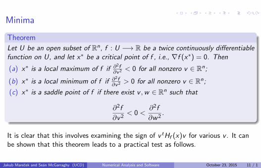
Let U be an open subset of Rn, f : U −→ R be a twice continuously differentiablefunction on U, and let x∗ be a critical point of f , i.e., ∇f (x∗) = 0. Then
(a) x∗ is a local maximum of f if ∂2f∂v2 < 0 for all nonzero v ∈ Rn;
(b) x∗ is a local minimum of f if ∂2f∂v2 > 0 for all nonzero v ∈ Rn;
(c) x∗ is a saddle point of f if there exist v ,w ∈ Rn such that
∂2f
∂v2< 0 <
∂2f
∂w2.
It is clear that this involves examining the sign of v tHf (x)v for various v . It canbe shown that this theorem leads to a practical test as follows.
Jakub Marecek and Sean McGarraghy (UCD) Numerical Analysis and Software October 23, 2015 11 / 1

The Approaches
Derivative-free methods
Gradient methods
Quasi-Newton methods
Newton-type methods
Interior-point methods
Jakub Marecek and Sean McGarraghy (UCD) Numerical Analysis and Software October 23, 2015 12 / 1

Derivative-Free Methods
For functions for x∗ ∈ Rn, the convergence of derivative-free methods is provablyslow.
Theorem (Nesterov)
For L-Lipschitz function f , ε ≤ 12L, and f provided as an oracle that allows f (x)
to be evaluated for x , derivative-free methods require(⌊L
2ε
⌋)n
calls to the oracle to reach ε accuracy.
Jakub Marecek and Sean McGarraghy (UCD) Numerical Analysis and Software October 23, 2015 13 / 1
Derivative-Free Methods
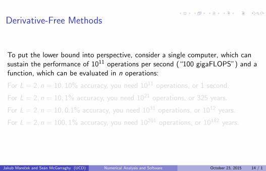
To put the lower bound into perspective, consider a single computer, which cansustain the performance of 1011 operations per second (“100 gigaFLOPS”) and afunction, which can be evaluated in n operations:
For L = 2, n = 10, 10% accuracy, you need 1011 operations, or 1 second.
For L = 2, n = 10, 1% accuracy, you need 1021 operations, or 325 years.
For L = 2, n = 10, 0.1% accuracy, you need 1031 operations, or 1012 years.
For L = 2, n = 100, 1% accuracy, you need 10201 operations, or 10182 years.
Jakub Marecek and Sean McGarraghy (UCD) Numerical Analysis and Software October 23, 2015 14 / 1

Derivative-Free Methods
To put the lower bound into perspective, consider a single computer, which cansustain the performance of 1011 operations per second (“100 gigaFLOPS”) and afunction, which can be evaluated in n operations:
For L = 2, n = 10, 10% accuracy, you need 1011 operations, or 1 second.
For L = 2, n = 10, 1% accuracy, you need 1021 operations, or 325 years.
For L = 2, n = 10, 0.1% accuracy, you need 1031 operations, or 1012 years.
For L = 2, n = 100, 1% accuracy, you need 10201 operations, or 10182 years.
Jakub Marecek and Sean McGarraghy (UCD) Numerical Analysis and Software October 23, 2015 14 / 1

Gradient Methods
Let us consider a local, unconstrained minimum x∗ of a multi-variate function,i.e., f (x∗) ≤ f (x)∀x with ||x − x∗|| ≤ ε.From the definition, at a local minimum x∗, we expect the variation in f due to asmall variation ∆x in x to be non-negative: ∇f (x∗)∆x =
∑ni=1
∂f (x∗)∂xi
∆x ≥ 0.
By considering ∆x coordinate wise, we get: ∇f (x∗) = 0.
Jakub Marecek and Sean McGarraghy (UCD) Numerical Analysis and Software October 23, 2015 15 / 1

Gradient Methods
In gradient methods, you consider xk+1 = xk − hk∇f (xk), where hk is one of:
Constant step hk = h or hk = h/√k + 1
Full relaxation hk = arg minh≥0 f (xk − h∇f (xk))
Armijo line search: find xk+1 such that the ratio ∇f (xk )(xk−xk+1)f (xk )−f (xk+1)
is within
some interval
Jakub Marecek and Sean McGarraghy (UCD) Numerical Analysis and Software October 23, 2015 16 / 1

Gradient Methods
For all of the choices above with f ∈ C 1,1L (Rn), one has
f (xk)− f (xk+1) ≥ ωL ||∇f (xk)||2. We hence want to bound the norm of the
gradient. It turns out:
kmini=0||∇f (xi )|| ≤
1√k + 1
[1
ωL (f (x0)− f ∗)
]1/2
This means that the norm of the gradient is less than ε, if the number ofiterations is greater than L
ωε2 (f (x0)− f ∗)− 1.
Jakub Marecek and Sean McGarraghy (UCD) Numerical Analysis and Software October 23, 2015 17 / 1

Gradient Methods
Theorem (Nesterov)
For f ∈ C 2,2M (Rn), lIn � H(f ∗) � LIn, a certain gradient method starting from
x0, r0 = ||x0 − x∗|| ≤ 2lM := r converges as follows:
||xk − x∗|| ≤ r r0
r − ρ0
(1− 2l
L + 3l
)k
This is called the (local) linear (rate of) convergence.
Jakub Marecek and Sean McGarraghy (UCD) Numerical Analysis and Software October 23, 2015 18 / 1

Newton-Type Methods
In finding a solution to a system of non-linear equations F (x) = 0,x ∈ Rn,F : Rn → Rn,
displacement ∆x as a solution to F (x) +∇F (x)∆x = 0, which is known as theNewton system.
Assuming [∇F ]−1 exists, we can use:
xk+1 = xk −[∇F (xk)
]−1F (xk).
When we move from finding zeros of F (x) to minimisingf (x), x ∈ Rn, f : Rn → R by finding zeros of ∇f (x) = 0, we obtain:
xk+1 = xk −[∇2f (xk)
]−1∇f (xk).
Jakub Marecek and Sean McGarraghy (UCD) Numerical Analysis and Software October 23, 2015 19 / 1

Newton-Type Methods
Alternatively, let us consider a quadratic approximation of f at point xk , i.e.,
f (xk) + 〈∇f (xk), x − xk〉+ 12〈H(xk)(x − xk), x − xk〉.
Assuming that H(xk) � 0, one should like to choose xk+1 by minimising theapproximation, i.e. solving
∇f (xk) + H(xk)(xk+1 − xk) = 0 for xk+1:
xk+1 = xk −[∇2f (xk)
]−1∇f (xk).
Jakub Marecek and Sean McGarraghy (UCD) Numerical Analysis and Software October 23, 2015 20 / 1
Newton-Type Methods
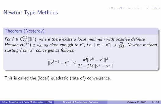
Theorem (Nesterov)
For f ∈ C 2,2M (Rn), where there exists a local minimum with positive definite
Hessian H(f ∗) � lIn, x0 close enough to x∗, i.e. ||x0 − x∗|| < 2l3M , Newton method
starting from x0 converges as follows:
||xk+1 − x∗|| ≤ M||xk − x∗||2
2l − 2M||xk − x∗||
This is called the (local) quadratic (rate of) convergence.
Jakub Marecek and Sean McGarraghy (UCD) Numerical Analysis and Software October 23, 2015 21 / 1

Newton-Type Methods
Newton method is only locally convergent, but the region of convergence is similarfor gradient and Newton methods.
One can try to address the possible divergence by considering damping:
xk+1 = xk − hk[∇2f (xk)
]−1∇f (xk), where hk ≥ 0 is a step-size, which usuallygoes to 1 as k goes to infinity, or other “regularisations”.
One can try to make a single iteration cheaper by either exploiting sparsity of theHessian or by considering some approximation of its inverse.
Jakub Marecek and Sean McGarraghy (UCD) Numerical Analysis and Software October 23, 2015 22 / 1

Quasi-Newton Methods
Quasi-Newton methods build up a sequence of approximations Hk of the inverseof the Hessian and use it in computing the step. Starting with H0 = In and somex0, in each iteration: xk+1 = xk + hkHk∇f (xk) for some step-length hk andHk+1 = Hk + ∆Hk where:
In rank-one methods, ∆Hk = (δk−Hkγk )(δk−Hkγk )T
〈δk−Hkγk ,γk 〉
In Broyden-Fletcher-Goldfarb-Shanno (BFGS):
∆Hk = Hkγk (δk )T +δk (γk )THk
〈Hkγk ,γk 〉 − βk Hkγk (γk )THk
〈Hkγk ,γk 〉
where δk = xk+1 − xk , γk = ∇f (xk+1)−∇f (xk), andβk = 1 + 〈γk , δk〉/〈Hkγk , γk〉. These methods are very successful in practice,although their rates of convergence are very hard to bound.
Jakub Marecek and Sean McGarraghy (UCD) Numerical Analysis and Software October 23, 2015 23 / 1

Lagrangian
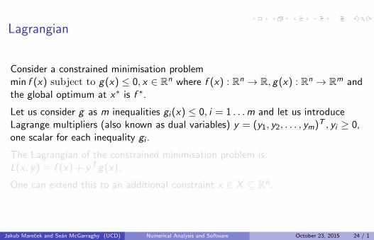
Consider a constrained minimisation problemmin f (x) subject to g(x) ≤ 0, x ∈ Rn where f (x) : Rn → R, g(x) : Rn → Rm andthe global optimum at x∗ is f ∗.
Let us consider g as m inequalities gi (x) ≤ 0, i = 1 . . .m and let us introduceLagrange multipliers (also known as dual variables) y = (y1, y2, . . . , ym)T , yi ≥ 0,one scalar for each inequality gi .
The Lagrangian of the constrained minimisation problem is:L(x , y) = f (x) + yTg(x).
One can extend this to an additional constraint x ∈ X ⊆ Rn.
Jakub Marecek and Sean McGarraghy (UCD) Numerical Analysis and Software October 23, 2015 24 / 1
Lagrangian
Consider a constrained minimisation problemmin f (x) subject to g(x) ≤ 0, x ∈ Rn where f (x) : Rn → R, g(x) : Rn → Rm andthe global optimum at x∗ is f ∗.
Let us consider g as m inequalities gi (x) ≤ 0, i = 1 . . .m and let us introduceLagrange multipliers (also known as dual variables) y = (y1, y2, . . . , ym)T , yi ≥ 0,one scalar for each inequality gi .
The Lagrangian of the constrained minimisation problem is:L(x , y) = f (x) + yTg(x).
One can extend this to an additional constraint x ∈ X ⊆ Rn.
Jakub Marecek and Sean McGarraghy (UCD) Numerical Analysis and Software October 23, 2015 24 / 1

Lagrangian
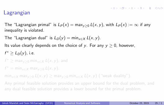
The “Lagrangian primal” is LP(x) = maxy≥0 L(x , y), with LP(x) :=∞ if anyinequality is violated.
The “Lagrangian dual” is LD(y) = minx∈X L(x , y).
Its value clearly depends on the choice of y . For any y ≥ 0, however,
f ∗ ≥ LD(y), i.e.
f ∗ ≥ maxy≥0 minx∈X L(x , y), and
f ∗ = minx∈X maxy≥0 L(x , y).
minx∈X maxy≥0 L(x , y) ≥ maxy≥0 minx∈X L(x , y) (“weak duality”).
Any primal feasible solution provides an upper bound for the dual problem, andany dual feasible solution provides a lower bound for the primal problem.
Jakub Marecek and Sean McGarraghy (UCD) Numerical Analysis and Software October 23, 2015 25 / 1

Lagrangian
The “Lagrangian primal” is LP(x) = maxy≥0 L(x , y), with LP(x) :=∞ if anyinequality is violated.
The “Lagrangian dual” is LD(y) = minx∈X L(x , y).
Its value clearly depends on the choice of y . For any y ≥ 0, however,
f ∗ ≥ LD(y), i.e.
f ∗ ≥ maxy≥0 minx∈X L(x , y), and
f ∗ = minx∈X maxy≥0 L(x , y).
minx∈X maxy≥0 L(x , y) ≥ maxy≥0 minx∈X L(x , y) (“weak duality”).
Any primal feasible solution provides an upper bound for the dual problem, andany dual feasible solution provides a lower bound for the primal problem.
Jakub Marecek and Sean McGarraghy (UCD) Numerical Analysis and Software October 23, 2015 25 / 1

Strong Duality and KKT Conditions
Assuming differentiability of L, Karush-Kuhn-Tucker (KKT) conditions arecomposed of stationarity (∇xL(x , y) = 0), primal feasibility (g(x) ≤ 0, x ∈ X ),dual feasibility (y ≥ 0), and“complementarity slackness” (yigi (x) = 0).
Under some “regularity” assumptions (also known as constraint qualifications), weare guaranteed that a point x satisfying the KKT condition exists.
If X ⊆ Rn is convex, f and g are convex, optimum f ∗ is finite, and the regularityassumptions hold, then we have
minx∈X maxy≥0 L(x , y) = maxy≥0 minx∈X L(x , y) (“strong duality”) and KKTconditions guarantee global optimality.
For example, Slater’s constraint qualifications is: ∃x ∈ int(X ) such that g(x) < 0.
If f and g are linear, no further constraint qualifications is needed and KKTconditions suffice.
Jakub Marecek and Sean McGarraghy (UCD) Numerical Analysis and Software October 23, 2015 26 / 1

Penalties and Barriers
Notice that the Lagrangian, as defined above, is not Lipschitz-continuous and isnot differentiable. Let us consider a closed set G defined by g , and let us assumeit has non-empty interior.
A penalty φ for G is a continuous function, such that φ(x) = 0 for any x ∈ G andφ(x) ≥ 0 for any x 6∈ G . E.g.
∑mi=1 max{gi (x), 0} (non-smooth),∑m
i=1(max{gi (x), 0})2 (smooth).
A barrier φ for G is a continuous function, such that φ(x)→∞ as x approachesthe boundary of G and is bounded from below elsewhere. E.g.∑m
i=11
(−gi (x))p , p ≥ 1 (power), −∑m
i=1 ln(−g(x)) (logarithmic).
One can consider (variants of) the Lagrangian of a constrained problem, whichinvolve a barrier for the inequalities.
Using such Lagrangians, one can develop interior-point methods.
Jakub Marecek and Sean McGarraghy (UCD) Numerical Analysis and Software October 23, 2015 27 / 1

Interior-Point Methods
Interior-point methods solve progressively less relaxed first-order optimalityconditions of a problem, which is equivalent to a constrained optimisation problemand uses barriers.
Consider a constrained minimisation min f (x) subject to g(x) ≤ 0 wheref (x) : Rn → R, g(x) : Rn → Rm are convex and twice differentiable.
A nonnegative slack variable z ∈ Rm can be used to replace the inequality byequality g(x) + z = 0.
Negative z can be avoided by using a barrier µ∑m
i=1 ln zi .
The (variant of) Lagrangian is: L(x , y , z ;µ) = f (x) + yT (g(x) + z)µ∑m
i=1 ln zi .
Jakub Marecek and Sean McGarraghy (UCD) Numerical Analysis and Software October 23, 2015 28 / 1

Interior-Point Methods
Now we can differentiate:
∇xL(x , y , z ;µ) =∇f (x) +∇g(x)T y (8.1)
∇yL(x , y , z ;µ) =g(x) + z (8.2)
∇zL(x , y , z ;µ) =yµZ−1e, (8.3)
where Z = diag(z1, z2, . . . , zm) and e = [1, 1, . . . 1]T .
Jakub Marecek and Sean McGarraghy (UCD) Numerical Analysis and Software October 23, 2015 29 / 1

Interior-Point Methods
The first-order optimality conditions obtained by setting the partial derivatives tozero are:
∇f (x) +∇g(x)T y = 0 (8.4)
g(x) + z = 0 (8.5)
YZe = µe (8.6)
y , z ≥ 0 (8.7)
where Y = diag(y1, y2, . . . , ym) and the parameter µ is reduced to 0 in the largenumber of iterations.
Jakub Marecek and Sean McGarraghy (UCD) Numerical Analysis and Software October 23, 2015 30 / 1

Interior-Point Methods
This can be solved using the Newton method, where at each step, one solves alinear system:[
−H(x , y) B(x)T
B(x) XY−1
] [∆x−∆y
]=
[∇f (x) + B(x)T y−g(x)− µY−1e
]where H(x , y) = ∇2f (x) +
∑mi=1 yi∇2gi (x) ∈ Rn×n and B(x) = ∇g(x) ∈ Rm×n.
This is a a saddle point system, which has often positive semidefinite A. Forconvex f , g , H(x, y) is positive semidefinite and diagonal matrix ZY 1 is alsopositive definite. A variety of methods works very well.
Jakub Marecek and Sean McGarraghy (UCD) Numerical Analysis and Software October 23, 2015 31 / 1

Condition Numbers
Assume the instance d := (A; b; c) is given. One can formalise the followingnotion, due to Renegar:
C (d) :=||d ||
inf{||∆d || : instance d + ∆d is infeasible or unbounded }.
The system (8.4–8.7) will have the condition number C (d)/µ.
Jakub Marecek and Sean McGarraghy (UCD) Numerical Analysis and Software October 23, 2015 32 / 1

Condition Numbers in Analyses
For a variety of methods, including:
Interior-point methods
Ellipsoid method
Perceptron method
Von Neumann method
assuming A is invertible, one can show a bound on the number of iterations islogarithmic in C (d).
This highlights the need for preconditioners.
Jakub Marecek and Sean McGarraghy (UCD) Numerical Analysis and Software October 23, 2015 33 / 1

Conclusions
Constrained optimisation is the work-horse of operations research.
Interior-point methods have been used on problems in dimensions 109.
Still, there are many open problems, including Smale’s 9th problem:
Is feasibility of a linear system of inequalities Ax ≥ b in P over reals,
i.e., solvable in polynomial time on the BSS machine?
Jakub Marecek and Sean McGarraghy (UCD) Numerical Analysis and Software October 23, 2015 34 / 1